Embed Size (px)
Citation preview

Leaning against the wind
Pierre-Olivier Weill∗
January 18, 2007
Abstract
During financial disruptions, marketmakers provide liquidity by absorbing external
selling pressure. They buy when the pressure is large, accumulate inventories, and sell
when the pressure alleviates. This paper studies optimal dynamic liquidity provision
in a theoretical market setting with large and temporary selling pressure, and order-
execution delays. I show that competitive marketmakers offer the socially optimal
amount of liquidity, provided they have access to sufficient capital. If raising capital
is costly, this suggests a policy role for lenient central-bank lending during financial
disruptions.
Keywords: marketmaking capital, marketmaker inventory management, financial cri-
sis.
∗Department of Economics, University of California, Los Angeles, 8283 Bunche, Box 951477, Los Angeles,CA, 90095, e-mail: [email protected]. First version: July 2003. This is the first chapter of myStanford PhD dissertation. I am deeply indebted to Darrell Duffie and Tom Sargent, for their supervision,their encouragements, many detailed comments and suggestions. I also thank Narayana Kocherlakota forfruitful discussions and suggestions. I benefited from comments by Manuel Amador, Andy Atkeson, MarcoBassetto, Bruno Biais, Vinicius Carrasco, John Y. Campbell, William Fuchs, Xavier Gabaix, Ed Green, BobHall, Ali Hortacsu, Steve Kohlhagen, Arvind Krishnamurthy, Hanno Lustig, Erzo Luttmer, Eva Nagypal,Lasse Heje Pedersen, Esteban Rossi-Hansberg, Tano Santos, Carmit Segal, Stijn Van Nieuwerburgh, FrancoisVelde, Tuomo Vuolteenaho, Ivan Werning, Randy Wright, Mark Wright, Bill Zame, Ruilin Zhou, participantsof Tom Sargent’s reading group at the University of Chicago, Stanford University 2003 SITE conference, andof seminar at Stanford University, NYU Economics and Stern, UCLA Anderson, Columbia GSB, HarvardUniversity, University of Pennsylvania, University of Michigan Finance, MIT Economics, the Universityof Minnesota, the University of Chicago, Northwestern University Economics and Kellogg, the Universityof Texas at Austin, the Federal Reserve Bank of Chicago, the Federal Reserve Bank of Cleveland, UCLAEconomics, the Federal Reserve Bank of Atlanta, THEMA, and MIT Sloan. The financial support of theKohlhagen Fellowship Fund at Stanford University is gratefully acknowledged. I am grateful to Andrea Prat(the editor) and two anonymous referees for comments that improved the paper. All errors are mine.
1

1 Introduction
When disruptions subject financial markets to unusually strong selling pressures, NYSE
specialists and NASDAQ marketmakers typically lean against the wind by absorbing the
market’s selling pressure and creating liquidity: they buy large quantity of assets and build
up inventories when selling pressure in the market is large, then dispose of those inventories
after that selling pressure has subsided.1 In this paper, I develop a model of optimal dynamic
liquidity provision. To explain how much and when liquidity should be provided, I solve for
socially optimal liquidity provision. I argue that some features of the socially optimal allo-
cation would be regarded by a policymaker as symptoms of poor liquidity provision. In fact,
these symptoms can be consistent with efficiency. I also show that when they can maintain
sufficient capital, competitive marketmakers supply the socially optimal amount of liquidity.
If capital-market imperfections prevent marketmakers from raising sufficient capital, this
suggests a policy role for lenient central-bank lending during financial disruptions.
The model studies the following scenario. In the beginning at time zero, outside investors
receive an aggregate shock which lowers their marginal utility for holding assets relative to
cash. This creates a sudden need for cash and induces a large selling pressure. Then,
randomly over time, each investor recovers from the shock, implying that the initial selling
pressure slowly alleviates. This is how I create a stylized representation of a “flight-to-
liquidity” (Longstaff [2004]) or a stock-market crash such as that of October 1987. All
trades are intermediated by marketmakers who do not derive any utility for holding assets
and who are located in a central marketplace which can be viewed, say, as the floor of the
New-York Stock Exchange. I assume that the asset market can be illiquid in the sense
that investors make contact with marketmakers only after random delays. This means that,
at each time, only a fraction of investors can trade, which effectively imposes an upper
limit on the fraction of outside orders marketmakers can execute per unit of time. The
random delays are designed to represent, for example, front-end order capture, clearing, and
settlement. While one expects such delays to be short in normal times, the Brady [1988]
report suggests that they were unusually long and variable during the crash of October
1987. Similarly, during the crash of October 1997, customers complained about “poor or
untimely execution from broker dealers” (SEC Staff Legal Bulletin No.8 of September 9,
1998). Lastly, McAndrews and Potter [2002] and Fleming and Garbade [2002] document
payment and transaction delays, due to disruption of the communication network after the
terrorist attacks of September 11, 2001.
1This behavior reflects one aspect of the U.S. Securities and Exchange Commission (SEC) Rule 11-b onmaintaining fair and orderly markets.
2

In this economic environment, marketmakers offer buyers and sellers quicker exchange,
what Demsetz [1968] called “immediacy”. Marketmakers anticipate that after the selling
pressure subsides, they will achieve contact with more buyers than sellers, which will allow
them then to transfer assets to buyers in two ways. They can either contact additional
sellers, which is time-consuming because of execution delays; or they can sell from their own
inventories, which can be done much more quickly. Therefore, by accumulating invento-
ries early, when the selling pressure is large, marketmakers mitigate the adverse impact on
investors of execution delays.
The socially optimal asset allocation maximizes the sum of investors’ and marketmakers’
intertemporal utility, subject to the order-execution technology. Because agents have quasi-
linear utilities, any other asset allocation could be Pareto improved by reallocating assets
and making time-zero consumption transfers. The upper panel of Figure 1 shows the socially
optimal time path of marketmakers’ inventory. (The associated parameters and modelling
assumptions are described in Section 2.) The graph shows that marketmakers accumulate
inventories only temporarily, when the selling pressure is large. Moreover, in this example, it
is not socially optimal that marketmakers start accumulating inventories at time zero when
the pressure is strongest. This suggests that a regulation forcing marketmakers to promptly
act as “buyers of last resort” could in fact result in a welfare loss. For example, if the initial
preference shock is sufficiently persistent, marketmakers acting as buyers of last resort will
end up holding assets for a very long time, which cannot be efficient given that they are not
the final holder of the asset. Lastly, when the economy is close to its steady state (interpreted
as a “normal time”) marketmakers should effectively act as “matchmakers” who never hold
assets but merely buy and re-sell instantly.
If marketmakers maintain sufficient capital, I show that the socially optimal allocation is
implemented in a competitive equilibrium, as follows. Investors can buy and sell assets only
when they contact marketmakers. Marketmakers compete for the order flow and can trade
among each other at each time. The lower panel of Figure 1 shows the equilibrium price
path. It jumps down at time zero, then increases, and eventually reaches its steady-state
level. A marketmaker finds it optimal to accumulate inventories only temporarily, when the
asset price grows at a sufficiently high rate. This growth rate compensates for the time value
of the money spent on inventory accumulation, giving a marketmaker just enough incentive
to provide liquidity. A marketmaker thus buys early at a low price and sells later at a high
price, but competition implies that the present value of her profit is zero.
Ample anecdotal evidence suggests that marketmakers do not maintain sufficient capital
(Brady [1988], Greenwald and Stein [1988], Mares [2001], and Greenberg [2003].) I find that
3

0 2 4 6 8 10 120
10
20
0 2 4 6 8 10 12
inventory
time
price
Figure 1: Features of the Competitive Equilibrium.
if marketmakers do not maintain sufficient capital, then they are not able to purchase as
many assets as prescribed by the socially optimal allocation. If capital-market imperfections
prevent marketmakers from raising sufficient capital before the crash, lenient central-bank
lending during the crash can improve welfare. Recall that during the crash of October 1987,
the Federal Reserve lowered the funds rate while encouraging commercial banks to lend to
security dealers (Parry [1997], Wigmore [1998].)
It is often argued that marketmakers should provide liquidity in order to maintain price
continuity and to smooth asset price movements.2 The present paper steps back from such
price-smoothing objective and instead studies liquidity provision in terms of the Pareto crite-
rion. The results indicate that Pareto-optimal liquidity provision is consistent with a discrete
price decline at the time of the crash. This suggests that requiring marketmakers to maintain
price continuity at the time of the crash might result in a welfare loss.
Related Literature
Liquidity provision in normal times has been analyzed in traditional inventory-based models
of marketmaking (see Chapter 2 of O’Hara [1995] for a review). Because they study inventory
management in normal times, these models assume exogenous, time-invariant supply and
demand curves. The present paper, by contrast, derives time-varying supply and demand
2For instance, the glossary of www.nyse.com states that NYSE specialists “use their capital to bridgetemporary gaps in supply and demand and help reduce price volatility.” See also the NYSE informationmemo 97-55.
4

curves from the solutions of investors’ inter-temporal utility maximization problems. This
allows to address the welfare impact of liquidity provision under unusual market conditions.
Another difference with this literature is that I study the impact of scarce marketmaking
capital on marketmakers’ profit and price dynamics.
In Grossman and Miller [1988] and Greenwald and Stein [1991], the social benefit of mar-
ketmakers’ liquidity provision is to share risk with sellers before the arrival of buyers. In the
present model, by contrast, the social benefit of liquidity provision is to facilitate trade, in
that it speeds up the allocation of assets from the initial sellers to the later buyers. Moreover
Grossman and Miller study a two-period model, which means that the timing of liquidity
provision is effectively exogenous. With its richer intertemporal structure, my model sheds
light on the optimal timing of liquidity provision.
Bernardo and Welch [2004] explain a financial-market crisis in a two-period model, along
the line of Diamond and Dybvig [1983], and they study the liquidity provision of myopic
marketmakers. The main objective of the present paper is not to explain the cause of a
crisis, but rather to develop an inter-temporal model of marketmakers optimal liquidity
provision, after an aggregate liquidity shock.
Search-and-matching models of financial markets study the impact of trading delays
in security markets (see, for instance, Duffie et al. [2005], Weill [2004], Vayanos and Wang
[2006], Vayanos and Weill [2006], Lagos [2006], Spulber [1996] and Hall and Rust [2003].)
The present model builds specifically on the work of Duffie, Garleanu and Perdersen. In
their model, marketmakers are matchmakers who, by assumption, cannot hold inventory.
By studying investment in marketmaking capacity, they focus on liquidity provision in the
long run. By contrast, I study liquidity provision in the short run and view marketmaking
capacity as a fixed parameter. In the short run, marketmakers provide liquidity by adjusting
their inventory positions.
Another related literature studies the equilibrium size of the middlemen sector in search-
and-matching economies, and provides steady-states in which the aggregate amount of mid-
dlemen’s inventories remains constant over time (see, among others, Rubinstein and Wolinsky
[1987], Li [1998], Shevchenko [2004], and Masters [2004]). The present paper studies inter-
mediation during a financial crisis, when it is arguably reasonable to take the size of the
marketmaking sector as given. In the short run, the marketmaking sector can only gain
capacity by increasing its capital and aggregate inventories fluctuate over time.
The remainder of this paper is organized as follows. Section 2 describes the economic
environment, Section 3 solves for socially optimal dynamic liquidity provision, Section 4
studies the implementation of this optimum in a competitive equilibrium, and introduces
5

borrowing-constrained marketmakers. Section 5 discusses policy implications, and Section 6
concludes. The appendix contains the proofs.
2 The Economic Environment
This section describes the economy and introduces the two main assumptions of this paper.
First, there is a large and temporary selling pressure. Second, there are order-execution
delays.
2.1 Marketmakers and Investors
Time is treated continuously, and runs forever. A probability space (Ω,F , P ) is fixed, as well
as an information filtration Ft, t ≥ 0 satisfying the usual conditions (Protter [1990]). The
economy is populated by a non-atomic continuum of infinitely lived and risk-neutral agents
who discount the future at the constant rate r > 0. An agent enjoys the consumption of a
non-storable numeraire good called “cash,” with a marginal utility normalized to 1.3
There is one asset in positive supply. An agent holding q units of the asset receives a
stochastic utility flow θ(t)q per unit of time. Stochastic variations in the marginal utility
θ(t) capture a broad range of trading motives such as changes in hedging needs, binding
borrowing constraints, changes in beliefs, or risk-management rules such as risk limits. There
are two types of agents, marketmakers and investors, with a measure one (without loss of
generality) of each. Marketmakers and investors differ in their marginal-utility processes
θ(t), t ≥ 0, as follows. A marketmaker has a constant marginal utility θ(t) = 0 while
an investor’s marginal utility is a two-state Markov chain: the high-marginal-utility state is
normalized to θ(t) = 1, and the low-marginal-utility state is θ(t) = 1− δ, for some δ ∈ (0, 1).
Investors transit randomly, and pair-wise independently, from low to high marginal utility
with intensity4 γu, and from high to low marginal utility with intensity γd.
These independent variations over time in investors’ marginal utilities create gains from
trade. A low-marginal-utility investor is willing to sell his asset to a high-marginal-utility
investor in exchange for cash. A marketmaker’s zero marginal utility could capture a large
exposure to the risk of the market she intermediates. In addition, it implies that in the
equilibrium to be described, a marketmaker will not be the final holder of the asset. In
particular, a marketmaker would choose to hold assets only because she expects to make
3Equivalently, one could assume that agents can borrow and save cash in some “bank account,” at theinterest rate r = r. Section 4 adopts this alternative formulation.
4For instance, if θ(t) = 1 − δ, the time infu ≥ 0 : θ(t+ u) 6= θ(t) until the next switch is exponentiallydistributed with parameter γu. The successive switching times are independent.
6

some profit by buying and reselling.5
Asset Holdings
The asset has s ∈ (0, 1) shares outstanding per investor’s capita. Marketmakers can hold any
positive quantity of the asset. The time t asset inventory I(t) of a representative marketmaker
satisfies the short-selling constraint6
I(t) ≥ 0. (1)
An investor also cannot short-sell and, moreover, he cannot hold more than one unit of the
asset. This paper restricts attention to allocations in which an investor holds either zero or
one unit of the asset. In equilibrium, because an investor has linear utility, he will find it
optimal to hold either the maximum quantity of one or the minimum quantity of zero.
An investor’s type is made up of his marginal utility (high “h,” or low “ℓ”) and his
ownership status (owner of one unit, “o,” or non-owner, “n”). The set of investors’ types
is T ≡ ℓo, hn, ho, ℓn. In anticipation of their equilibrium behavior, low-marginal-utility
owners (ℓo) are named “sellers,” and high-marginal-utility non-owners (hn) are “buyers.”
For each σ ∈ T , µσ(t) denotes the fraction of type-σ investors in the total population of
investors. These fractions must satisfy two accounting identities. First, of course,
µℓo(t) + µhn(t) + µℓn(t) + µho(t) = 1. (2)
Second, the assets are held either by investors or marketmakers, so
µho(t) + µℓo(t) + I(t) = s. (3)
2.2 Crash and Recovery
I select initial conditions representing the strong selling pressure of a financial disruption.
Namely, it is assumed that, at time zero, all investors are in the low-marginal-utility state
(see Table 1). Then, as earlier specified, investors transit to the high-marginal-utility state.
Under suitable measurability requirements (see Sun [2000], Theorem C), the law of large
5The results of this paper hold under the weaker assumption that marketmakers’ marginal utility isθ(t) = 1 − δM , for some holding cost δM > δ. Proofs are available from the author upon request.
6The short-selling constraint means that both marketmakers and investors face an infinite cost of holdinga negative asset position. This may be viewed as a strong assumption because it is typically easier formarketmakers to go short than for investors. However, one can show that, in the present setup, marketmakersfind it optimal to choose I(t) ≥ 0, as long as they incur a finite but sufficiently large cost c > 1−δγd/(r+ρ+γu + γd) per unit of negative inventory. This cost could capture, for example, the fact that short positionsare more risky than long positions.
7
numbers applies, and the fraction µh(t) ≡ µho(t) + µhn(t) of high-marginal-utility investors
solves the ordinary differential equation (ODE)
µh(t) = γu(
µℓo(t) + µℓn(t))
− γd(
µho(t) + µhn(t))
= γu(
1 − µh(t))
− γdµh(t)
= γu − γµh(t), (4)
where µh(t) = dµh(t)/dt and γ ≡ γu + γd. The first term in (4) is the rate of flow of
low-marginal-utility investors transiting to the high-marginal-utility state, while the second
term is the rate of flow of high-marginal-utility investors transiting to the low-marginal-utility
state. With the initial condition µh(0) = 0, the solution of (4) is
µh(t) = y(
1 − e−γt)
, (5)
where y ≡ γu/γ is the steady-state fraction of high-marginal-utility investors. Importantly
for the remainder of the paper, it is assumed that
s < y. (6)
In other words, in steady state, the fraction y of high-marginal-utility investors exceeds the
asset supply s. This will ensure that, asymptotically in equilibrium, the selling pressure has
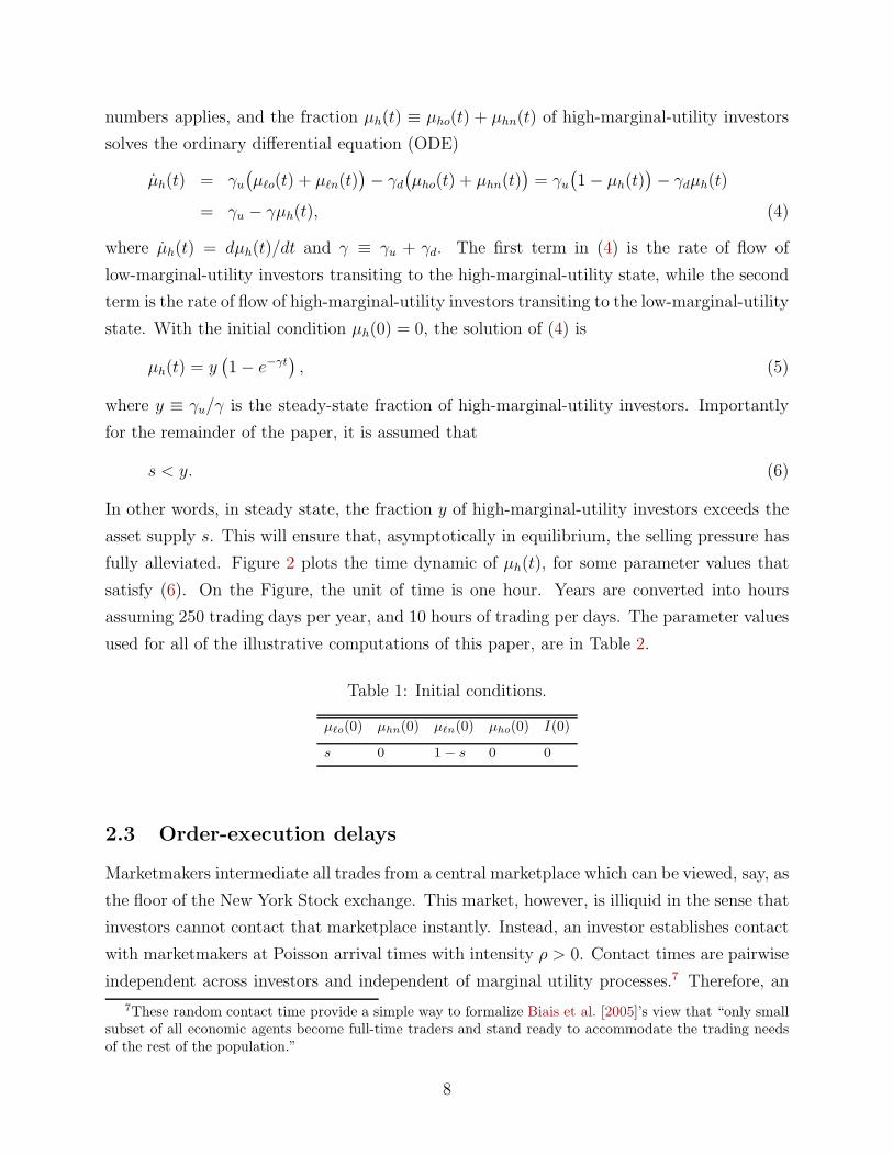
fully alleviated. Figure 2 plots the time dynamic of µh(t), for some parameter values that
satisfy (6). On the Figure, the unit of time is one hour. Years are converted into hours
assuming 250 trading days per year, and 10 hours of trading per days. The parameter values
used for all of the illustrative computations of this paper, are in Table 2.
Table 1: Initial conditions.
µℓo(0) µhn(0) µℓn(0) µho(0) I(0)
s 0 1 − s 0 0
2.3 Order-execution delays
Marketmakers intermediate all trades from a central marketplace which can be viewed, say, as
the floor of the New York Stock exchange. This market, however, is illiquid in the sense that
investors cannot contact that marketplace instantly. Instead, an investor establishes contact
with marketmakers at Poisson arrival times with intensity ρ > 0. Contact times are pairwise
independent across investors and independent of marginal utility processes.7 Therefore, an
7These random contact time provide a simple way to formalize Biais et al. [2005]’s view that “only smallsubset of all economic agents become full-time traders and stand ready to accommodate the trading needsof the rest of the population.”
8

0 5 10 150
0.1
0.2
0.3
0.4
µh(t)
s
time (hours)
Figure 2: Dynamic of µh(t).
Table 2: Parameter Values.
Parameters Value
Measure of Shares s 0.2Discount Rate r 5%Contact Intensity ρ 1000Intensity of Switch to High γu 90Intensity of Switch to Low γd 10Low marginal utility 1 − δ 0.01
Time is measured in years. Assuming that the stock market opens250 days a year, ρ = 1000 means that it takes 2.5 hours to executean order, on average. The parameter γ = γu + γd measures thespeed of the recovery. Specifically, with γ = 100, µh(t) reacheshalf of its steady-state level in about 1.73 days.
application of the law of large numbers (under the technical conditions mentioned earlier)
implies that contacts between type-σ investors and marketmakers occur at a total (almost
sure) rate of ρµσ(t). Hence, during a small time interval of length ε, marketmakers can only
execute a fixed fraction ρε of randomly chosen orders originating from type-σ investors.8
The random contact times represent a broad range of execution delays, including the time
to contact a marketmaker, to negotiate and process an order, to deliver an asset, or to transfer
a payment. One might argue that such execution delays are usually quite short and perhaps
therefore of little consequence to the quality of an allocation. The Brady [1988] report
shows, however, that during the October 1987 crash, overloaded execution systems created
8Instead of imposing a limit on the fraction of orders that marketmakers can execute per unit of time,one could impose a limit on the total number of orders they can execute. One can show that, under such analternative specification, competitive marketmakers also provide the socially optimal amount of liquidity.
9

delays that were much longer and variable than in normal times. It suggests that these
delays might have amplified liquidity problems in a far-from-negligible manner. Although
the trading technology improved after the crash of October 1987, substantial execution
delays also occurred during the crash of October 1997. The SEC reported that “broker-
dealers web servers had reached their maximum capacity to handle simultaneous users” and
“telephone lines were overwhelmed with callers who were frustrated by the inability to access
information online.” As a result of these capacity problems, customers could not be “routed
to their designated market center for execution on a timely basis” and “a number of broker
dealers were forced to manually execute some customers orders.”9
3 Optimal Dynamic Liquidity Provision
The first objective of this section is to explain the benefit of liquidity provision, addressing
how much and when liquidity should be provided. Its second objective is to establish a
benchmark against which to judge the market equilibria studied in Sections 4 and 4.2. To
these ends, I temporarily abstract from marketmakers’ incentives to provide liquidity and
solve for socially optimal allocations, maximizing the sum of investors and marketmakers’
intertemporal utility, subject to order-execution delays. The optimal allocation is found to
resemble “leaning against the wind.” Namely, it is socially optimal that a marketmaker
accumulates inventories when the selling pressure is strong.
3.1 Asset Allocations
At each time, a representative marketmaker can transfer assets only to her own account
or among those of investors who are currently contacting her. For instance, the flow rate
uℓ(t) of assets that a marketmaker takes from low-marginal-utility investors is subject to the
order-flow constraint
−ρµℓn(t) ≤ uℓ(t) ≤ ρµℓo(t). (7)
The upper (lower) bound shown in (7) is the flow of ℓo (ℓn) investors who establish contact
with marketmakers at time t. Similarly, the flow uh(t) of assets that a marketmaker transfers
to high-marginal-utility investors is subject to the order-flow constraint
−ρµho(t) ≤ uh(t) ≤ ρµhn(t). (8)
9SEC Staff Legal Bulletin No.8, http://www.sec.gov/interps/legal/slbmr8.htm
10

When the two flows uℓ(t) and uh(t) are equal, a marketmaker is a matchmaker, in the sense
that she takes assets from some ℓo investors (sellers) and transfers them instantly to some hn
investors (buyers). If the two flows are not equal, a marketmaker is not only matching buyers
and sellers, but she is also changing her inventory position. For example, if both uℓ(t) and
uh(t) are positive, a marketmaker is matching sellers and buyers at the rate minuℓ(t), uh(t).The net flow uℓ(t)−uh(t) represents the rate of change of a marketmaker’s inventory, in that
I(t) = uℓ(t) − uh(t). (9)
Similarly, the rate of change of the fraction µℓo(t) of low-marginal-utility owners is
µℓo(t) = −uℓ(t) − γuµℓo(t) + γdµho(t), (10)
where the terms γuµℓo(t) and γdµho(t) reflect transitions of investors from low to high
marginal utility, and from high to low marginal utility, respectively. Likewise, the rate
of change of the fractions of hn, ℓn, and ho investors are, respectively,
µhn(t) = −uh(t) − γdµhn(t) + γuµℓn(t) (11)
µℓn(t) = uℓ(t) − γuµℓn(t) + γdµhn(t) (12)
µho(t) = uh(t) − γdµho(t) + γuµℓo(t). (13)
Definition 1 (Feasible Allocation). A feasible allocation is some distribution µ(t) ≡(
µσ(t))
σ∈Tof types, some inventory holding I(t), and some piecewise continuous asset flows u(t) ≡(
uh(t), uℓ(t))
such that
(i) At each time, the short-selling constraint (1) and the order-flow constraints (7)-(8) are
satisfied.
(ii) The ODEs (9)-(13) hold.
(iii) The initial conditions of Table 1 hold.
Since u(t) is piecewise continuous, µ(t) and I(t) are piecewise continuously differentiable. A
feasible allocation is said to be constrained Pareto optimal if it cannot be Pareto improved by
choosing another feasible allocation and making time-zero cash transfers. As it is standard
with quasi-linear preferences, it can be shown that a constrained Pareto optimal allocation
must maximize∫ +∞
0
e−rt(
µho(t) + (1 − δ)µℓo(t)
)
dt, (14)
11

the equally weighted sum of investors’ intertemporal utilities for holding assets.10 This
criterion is deterministic, reflecting pairwise independence of investors’ marginal-utility and
contact-time processes. Conversely, an asset allocation maximizing (14) is constrained Pareto
optimal. This discussion motivates the following definition of an optimal allocation.
Definition 2 (Socially Optimal Allocation). A socially optimal allocation is some feasible
allocation maximizing (14).
3.2 The Benefit of Liquidity Provision
This subsection illustrates the social benefits of accumulating inventories. Namely, it consid-
ers the no-inventory allocation (I(t) = 0, at each time), and shows that it can be improved if
marketmakers accumulate a small amount of inventory, when the selling pressure is strong.
I start by describing some features of the no-inventory allocation. Substituting I(t) = 0 into
equation (3) gives
µℓo(t) = s− µh(t) + µhn(t). (15)
The “crossing time” is the time ts at which µh(ts) = s. This is, as Figure 2 illustrates, the
time at which the fraction µh(t) of high-marginal-utility investors crosses the supply s of
assets. Because µh(t) is increasing, equation (15) implies that
ρµhn(t) < ρµℓo(t) (16)
if and only if t < ts. Therefore, in the no-inventory allocation, before the crossing time, the
selling pressure is “positive,” meaning that marketmakers are in contact with more sellers
(ℓo) than buyers (hn). After the crossing time, they are in contact with more buyers than
sellers.
Intuitively, the no-inventory allocation can be improved as follows. A marketmaker can
take an additional asset from a seller before the crossing time, say at t1 = ts−ε, and transfer
it to some buyer after the crossing time, at t2 = ts + ε. Because the transfer occurs around
the crossing time, the transfer time 2ε can be made arbitrarily small.
The benefit is that, for a sufficiently small ε, this asset is allocated almost instantly
to some high-marginal-utility investor. Without the transfer, by contrast, this asset would
continue to be held by a low-marginal-utility investor until either i) the seller transits to
a high marginal utility with intensity γu, or ii) the seller establishes another contact with
10Marketmakers intertemporal utility for holding assets is equal to zero and hence does not appear in(14). If a marketmaker marginal utility for holding asset is (1 − δM ) > 0, then one has to add a term∫
∞
0e−rt(1 − δM )I(t) dt to the above criterion.
12

0 5 10 15
0
10
30
time (hours)
I(t)/s (%)
t1 t2
m/s
Figure 3: Illustrative Buffer Allocations.
a marketmaker with intensity ρ. This means that, without the transfer, this asset would
continue to be held by a seller and not by a buyer, with an instantaneous utility cost of δ,
incurred for a non-negligible average time of 1/(γu + ρ).
The cost of the transfer is that the asset is temporarily held by a marketmaker and not
by a seller, implying an instantaneous utility cost of 1− δ. If ε is sufficiently small, this cost
is incurred for a negligible time and is smaller than the benefit. This intuitive argument can
be formalized by studying the following family of feasible allocations.
Definition 3 (Buffer Allocation). A buffer allocation is a feasible allocation defined by two
times (t1, t2) ∈ [0, ts] × [ts,+∞), called “breaking times,” such that
uℓ(t) = ρµhn(t) and uh(t) = ρµhn(t) t ∈ [0, t1)
uℓ(t) = ρµℓo(t) and uh(t) = ρµhn(t) t ∈ [t1, t2]
uℓ(t) = ρµℓo(t) and uh(t) = ρµℓo(t), t ∈ (t2,∞],
and I(t2) = 0.
The no-inventory allocation is the buffer allocation for which t1 = t2 = ts. A buffer allocation
has the “bang-bang” property: at each time, either uℓ(t) = ρµℓo(t) or uh(t) = ρµhn(t).
Because of the linear objective (14), it is natural to guess that a socially optimal allocation
will also have this bang-bang property. In the next subsection, Theorem 1 will confirm
this conjecture, showing that the socially optimal allocation belongs to the family of buffer
allocations.
In a buffer allocation, a marketmaker acts as a “buffer,” in that she accumulates assets
when the selling pressure is strong and unwinds these trades when the pressure alleviates.
13

Specifically, as illustrated in Figure 3, a buffer allocation (t1, t2) has three phases. In the first
phase, when t ∈ [0, t1], a marketmaker does not accumulate inventory (uℓ(t) = uh(t) and
I(t) = 0). In the second phase, when t ∈ (t1, t2), a marketmaker first builds up (uℓ(t) > uh(t)
and I(t) > 0) and then unwinds (uℓ(t) < uh(t) and I(t) > 0) her inventory position. At
time t2, her inventory position reaches zero. In the third phase t ∈ [t2,+∞), a marketmaker
does not accumulate inventory (uℓ(t) = uh(t) and I(t) = 0). The following proposition
characterizes buffer allocations by the maximum inventory position held by marketmakers.
Proposition 1. There exist some m ∈ R+, some strictly decreasing continuous function
ψ : [0, m] → R+, and some strictly increasing continuous functions φi : [0, m] → R+,
i ∈ 1, 2, such that, for all m ∈ [0, m] and all buffer allocations (t1, t2),
m = maxt∈R+
I(t) and ψ(m) = arg maxt∈R+
I(t) (17)
t1 = ψ(m) − φ1(m) and t2 = ψ(m) + φ2(m), (18)
where m is the unique solution of ψ(z) − φ1(z) = 0. Furthermore, ψ(0) = ts and φ1(0) =
φ2(0) = 0.
In words, the breaking times (t1, t2) of a buffer allocation can be written as functions of the
maximum inventory position m. The maximum inventory position is achieved at time ψ(m).
In addition, the larger is a marketmaker’s maximum inventory position, the earlier she starts
to accumulate and the longer she accumulates. Lastly, if she starts to accumulate at time
zero, then her maximum inventory position is m.
The social welfare (14) associated with a buffer allocation can be written as W (m), for
some function W ( · ) of the maximum inventory position m. As anticipated by the intuitive
argument, one can prove the following result.
Proposition 2.
limm→0+
W (m) −W (0)
m> 0. (19)
This demonstrates that the no-inventory allocation (m = 0) is improved by accumulating a
small amount of inventory near the crossing time ts.
3.3 The Socially Optimal Allocation
Having shown that accumulating some inventory improves welfare, this section explains how
much inventory marketmakers should accumulate. Namely, it provides first-order sufficient
conditions for, and solves for, a socially optimal allocation. The reader may wish to skip the
14

following paragraph on first-order conditions, and go directly to Theorem 1, which describes
the socially optimal allocation.
First-Order Sufficient Conditions
The first-order sufficient conditions are based on Seierstad and Sydsæter [1977]. The ac-
counting identities µho(t) = µh(t) − µhn(t) and µℓn(t) = 1 − µh(t) − µℓn(t) are substituted
into the objective and the constraints, reducing the state variables to(
µℓo(t), µhn(t), I(t))
.
The “current-value” Lagrangian (see Kamien and Schwartz [1991], Part II, Section 8) is
L(t) = µh(t) − µhn(t) + (1 − δ)µℓo(t) (20)
+ λℓ(t)(
−uℓ(t) − γuµℓo(t) − γdµhn(t) + γdµh(t))
−λh(t)(
−uh(t) − γuµℓo(t) − γdµhn(t) + γu(1 − µh(t)))
+ λI(t)(
uℓ(t) − uh(t))
+wℓ(t)(
ρµℓo(t) − uℓ(t))
+ wh(t)(
ρµhn(t) − uh(t))
+ ηI(t) I(t).
The multiplier λℓ(t) of the ODE (10) represents the social value of increasing the flow of
investors from the ℓn type to the ℓo type or, equivalently, the value of transferring an asset
to an ℓn investor. One gives a similar interpretation to the multipliers λh(t) and λI(t) of the
ODEs (11) and (9), respectively.11 The multipliers wℓ(t) and wh(t) of the flow constraints (7)
and (8) represent the social value of increasing the rate of contact with ℓo and hn investors,
respectively.12 The multiplier on the short-selling constraint (1) is ηI(t). The first-order
condition with respect to the controls uℓ(t) and uh(t) are
wℓ(t) = λI(t) − λℓ(t) (21)
wh(t) = λh(t) − λI(t), (22)
respectively. For instance, (21) decomposes wℓ(t) into the opportunity cost −λℓ(t) of taking
assets from ℓo investors, and the benefit λI(t) of increasing a marketmaker’s inventory. The
positivity and complementary-slackness conditions for wℓ(t) and wh(t), respectively, are
wℓ(t) ≥ 0 and wℓ(t)(
ρµℓo(t) − uℓ(t))
= 0, (23)
wh(t) ≥ 0 and wh(t)(
ρµhn(t) − uh(t))
= 0. (24)
The multipliers wℓ(t) and wh(t) are non-negative because a marketmaker can ignore addi-
tional contacts. The complementary-slackness condition (23) means that, when the marginal
11In equation (20), the minus sign in front of λh(t) is contrary to conventional notations but turns out tosimplify the exposition.
12It is anticipated that the left-hand constraints in (7) and (8) never bind. In other words, a marketmakernever transfers asset from a high-marginal-utility to a low-marginal-utility investor.
15

value wℓ(t) of additional contact is strictly positive, a marketmaker should take the assets
of all ℓo investors with whom she is currently in contact. One also has the positivity and
complementary-slackness conditions
ηI(t) ≥ 0 and ηI(t)I(t) = 0. (25)
The ODE for the the multipliers λℓ(t), λh(t), and λI(t) are
rλℓ(t) = 1 − δ + γu(λh(t) − λℓ(t)) + ρwℓ(t) + λℓ(t) (26)
rλh(t) = 1 + γd(λℓ(t) − λh(t)) − ρwh(t) + λh(t) (27)
rλI(t) = ηI(t) + λI(t), (28)
respectively. For instance, (26) decomposes the flow value rλℓ(t) of transferring an asset to
a low-marginal-utility investor. The first term, 1 − δ, is the flow marginal utility of a low-
marginal-utility investor holding one unit of the asset. The second term, γu(
λh(t)−λℓ(t))
, is
the expected rate of net utility associated with a transition to high marginal utility. That is,
with intensity γu, λℓ(t) becomes the value λh(t) of transferring an asset to a high-marginal-
utility investor. The third term, ρwℓ(t), is the expected rate of net utility of a contact
between an ℓo investor and a marketmaker. The multipliers(
λℓ(t), λh(t), λI(t))
must satisfy
the following additional restrictions. First, they must satisfy the transversality conditions
that λℓ(t)e−rt, λh(t)e
−rt, and λI(t)e−rt go to zero as time goes to infinity. Second, the
multipliers λh(t) and λℓ(t) are continuous. Because the control variable u(t) does not appear
in the short-selling constraint I(t) ≥ 0, however, the multiplier λI(t) might jump, with the
restriction that
λI(t+) − λI(t
−) ≤ 0 if I(t) = 0. (29)
In other words, the multiplier λI(t) can jump down, but only when the short-selling con-
straint is binding. Intuitively, if λI(t) were to jump up at t, a marketmaker could accu-
mulate additional inventory shortly before t, say a quantity ε, improving the objective by
ε(
λI(t+) − λI(t
−))
e−rt.13
The Socially Optimal Allocation
Appendix B guesses and verifies that the (essentially unique) socially optimal allocation is
a buffer allocation. Namely, for a given buffer allocation, one constructs multipliers solving
13Because the ODEs for the state variables are linear, the first-order sufficient conditions impose no signrestriction on the multipliers λh(t), λℓ(t), and λI(t) (see Section 3 in Part II of Kamien and Schwartz [1991]).
16

the first-order conditions (21) through (29). The restriction wℓ(t1) = 0 is used to find the
breaking-times t1 and t2.
Theorem 1 (Socially optimal Allocation). There exists a socially optimal allocation(
µ∗(t), I∗(t), u∗(t), t ≥ 0)
. This allocation is a buffer allocation with breaking times (t∗1, t∗2)
determined by
e−γt∗
1 =
(
1 − s
y
)
1 − e−ρ∆∗
ρ
ρ− γ
e−γ∆∗ − e−ρ∆∗(30)
t∗2 = t∗1 + ∆∗ (31)
∆∗ = min
1
r + ρlog
(
1 +δ(r + ρ)
γu + (1 − δ)(r + ρ+ γd)
)
, ∆
,
where ∆ ≡ φ1(m) + φ2(m) and, if γ = ρ, one lets (e−γx − e−ρx)/(ρ− γ) ≡ x for all x ∈ R.
If ∆∗ = ∆, the first breaking time is t∗1 = 0, meaning that a marketmaker starts accumulating
inventory at the time of the “crash.”
The socially optimal allocation has three main features. First, it is optimal that a market-
maker provides some liquidity: From time t∗1 to time t∗2, she builds up and unwinds a positive
inventory position. Second, it is not necessarily optimal that a marketmaker provides liq-
uidity at time zero, when the selling pressure is strongest. This suggests that, although a
marketmaker should provide liquidity, she should not act as a “buyer of last resort.” Third,
when the economy is close to its steady state, interpreted as a normal time, a marketmaker
should act as a mere matchmaker, meaning that she should buy and sell instantly. Thus, the
socially optimal allocation draws a sharp distinction between socially optimal marketmaking
in a normal time of low selling pressure, versus a bad time of strong selling pressure.14
4 Market Equilibrium
This section studies marketmakers’ incentives to provide liquidity. I show that the socially
optimal allocation can be implemented in a competitive equilibrium as long as marketmakers
have access to sufficient capital.
4.1 Competitive Marketmakers
This subsection describes a competitive market structure that implements the socially opti-
mal allocation.
14Weill [2006] shows that the above socially optimal allocation is unique and provides natural comparativestatics. It also establishes that, as ρ → ∞ and the trading frictions vanish, the socially optimal allocationconverges to a Walrasian limit in which marketmakers do not hold any inventories.
17

It is assumed that a marketmaker has access to some bank account earning the constant
interest rate r = r. At each time t, she buys a flow uℓ(t) ∈ R+ of assets, sells a flow
uh(t) ∈ R+, and consumes cash at the positive rate c(t) ∈ R+. She takes as given the asset
price path
p(t), t ≥ 0
. Hence, her bank account position a(t) and her inventory position
I(t) evolve according to
a(t) = ra(t) + p(t)(
uh(t) − uℓ(t))
− c(t) (32)
I(t) = uℓ(t) − uh(t). (33)
In addition, she faces the borrowing and short-selling constraints
a(t) ≥ 0 (34)
I(t) ≥ 0. (35)
Lastly, at time zero, a marketmaker holds no inventory (I(0) = 0) and maintains a strictly
positive amount of capital, a(0). This subsection restricts attention to some large a(0), in
the sense that the borrowing constraint (34) does not bind in equilibrium. (This statement is
made precise by Theorem 2 and Proposition 3.) The marketmaker’s objective is to maximize
the present value
∫ +∞
0
e−rtc(t) dt (36)
of her consumption stream with respect to
a(t), I(t), uℓ(t), uh(t), c(t), t ≥ 0
, subject to the
constraints (32)-(35), and the constraint that uℓ(t) and uh(t) are piecewise continuous.
Let’s turn to the investor’s problem. An investor establishes contact with the marketplace
at Poisson arrival times with intensity ρ > 0.15 Conditional on establishing contact at time
t, he can buy or sell the asset at price p(t). I solve the investor’s problem using a “guess
and verify” method. Specifically, I guess that, in equilibrium, an ℓo (hn) investor always
finds it weakly optimal to sell (buy). If an ℓo (hn) investor is indifferent between selling and
not selling, he might choose not to sell (buy). Lastly, I guess that investors of types ℓn and
ho never trade. The time-t continuation utility of an investor of type σ ∈ T who follows
this policy is denoted Vσ(t). Hence, a seller’s reservation value is ∆Vℓ(t) ≡ Vℓo(t) − Vℓn(t),
the net value of holding one asset rather than none, while following the candidate optimal
trading strategy. Likewise, a buyer’s reservation value is ∆Vh(t) ≡ Vho(t)−Vhn(t). Appendix
15In the alternative market setting of Duffie, Garleanu and Pedersen (2005), each investors bargain in-dividually with a marketmaker who can trade assets instantly on a competitive inter-dealer market. Thismarket setting is equivalent to the present one in the special case in which the bargaining strength of amarketmaker is equal to zero.
18

C provides ODEs for these continuation utilities and reservation values, as well as a precise
definition of a competitive equilibrium. The main result of this subsection states that the
optimal allocation can be implemented in some equilibrium:
Theorem 2 (Implementation). There exists some a∗0 ∈ R+ such that, for all a(0) ≥ a∗0,
there exists a competitive equilibrium whose allocation is the optimal allocation.
The proof identifies the price and the reservation values with the Lagrange multipliers of the
socially optimal allocation (see Table 3). For instance, the asset price p(t) is equal to the
multiplier λI(t) for the ODE I(t) = uℓ(t)−uh(t), interpreted as the social value of increasing
the inventory position of a marketmaker. Also, Table 3 and the complementary slackness
condition (23) imply that, before the first breaking time t∗1, wℓ(t) = p(t) − ∆Vℓ(t) = 0. In
other words, because the socially optimal allocation prescribes that marketmakers do not
accommodate the selling pressure, the social value wℓ(t) of increasing the rate of contact with
sellers is zero. In equilibrium, this means that the price adjusts so that sellers are indifferent
between selling and not selling.
Weill [2006] shows, without characterizing the equilibrium allocation, that the efficiency
result of Theorem 2 generalizes to environments with aggregate uncertainty and non-linear
utility flow for holding the assets as long as: i) agents have quasi-linear utility, meaning that
they enjoy the consumption of some numeraire good with a constant marginal utility of 1,
and ii) the probability distribution of an investor’s contact times with the market does not
depend on other agents’ trading strategies.16
Equilibrium Price Path and Marketmakers’ Incentive
Appendix B.2 derives closed-form solutions for the equilibrium price path p(t) and the reser-
vation values ∆Vℓ(t) and ∆Vh(t). The price path, shown in the lower panel of Figure
4, jumps down at time zero, then increases, and eventually stabilizes at its steady-state
level.17 The price path reflects the three phases of the socially optimal allocation: before
the first breaking time t∗1, sellers are indifferent between selling or not selling, meaning that
p(t) = ∆Vℓ(t) = λℓ(t). Moreover, equation (26) shows that the growth rate p(t)/p(t) of the
price is strictly less than r− (1− δ)/p(t). This is because a seller with marginal utility 1− δ
16Assumption ii) would fail, for instance, in a model with congestions, when the intensity of contact withmarketmakers is a decreasing function of the number of agents on the same side of the market. In that case,an optimal allocation would be implemented in a different competitive setting, in the spirit of Moen [1997]and Shimer [1995]’s competitive-search models.
17A simple way to construct the initial price jump is to start the economy in steady state at t = 0 andassume that agents anticipate a crash at some Poisson arrival time with intensity κ. One can show thatthe results of this paper would apply, provided that either κ is small enough or t∗
1> 0. For Figure 4, it is
assumed that κ = 0.
19

Table 3: Identifying Prices with Multipliers.
Equilibrium Objects Multipliers Constraints
p(t) λI(t) I(t) = uℓ(t) − uh(t)
∆Vℓ(t) λℓ(t) µℓo(t) = −uℓ(t) . . .
p(t) − ∆Vℓ(t) wℓ(t) uℓ(t) ≤ ρµℓo(t)
∆Vh(t) λh(t) µhn(t) = −uh(t) . . .
∆Vh(t) − p(t) wh(t) uh(t) ≤ ρµhn(t)
In a given row, the equilibrium object in the first column isequal to the Lagrange multiplier in the second column. Thethird column describes the constraints associated with these mul-tipliers. For instance, in the first row, the price p(t) (first col-umn) is equal to the multiplier λI(t) (second column) of the ODEI(t) = uℓ(t) − uh(t) (third column).
does not need a large capital gain to be willing to hold the asset. By contrast, in between
the two breaking times t∗1 and t∗2, marketmakers accommodate all of the selling pressure.
As a result, the “marginal investor” is a marketmaker and p(t) > ∆Vℓ(t), meaning that the
liquidity provision of marketmakers raises the asset price above a seller’s reservation value.
Moreover, equation (28) shows that the price grows at the higher rate p(t)/p(t) = r, implying
that the price recovers more quickly when marketmakers provide liquidity.
The capital gain during [t∗1, t∗2] exactly compensates a marketmaker for the time value of
cash spent on liquidity provision. In other words, a marketmaker is indifferent between i)
investing cash in her bank account, and ii) buying assets after t∗1 and selling them before
t∗2. Before t∗1 and after t∗2, however, the capital gain is strictly smaller than r, making
it unprofitable for a marketmaker to buy the asset on her own account. Therefore, in
equilibrium, a marketmaker’s intertemporal utility is equal to a(0), the value of her time-
zero capital. In other words, although a marketmaker buys low and sells high, competition
drives the present value of her profit to zero.
The equilibrium of Theorem 2 implements a socially optimal allocation with a bid-ask
spread of zero. Conversely, Weill [2006] shows that, if marketmakers could bargain individ-
ually with investors and charge a strictly positive bid-ask spread, then they would provide
more liquidity than is socially optimal. However, this finding that efficiency requires a zero
bid-ask spread crucially depends on the specification of the trading friction. For example,
Weill [2006] shows that if marketmakers face a fixed upper limit on the total number of orders
they can execute per unit of times then the equilibrium liquidity provision would continue
20

0 4 6 10 12
t∗1 t∗2
p(t)
∆Vh(t)
∆Vℓ(t)
I(t)
Figure 4: The Equilibrium Price Path.
to be socially optimal, but the equilibrium bid-ask spread would be strictly positive.
One might wonder whether the present results survive the introduction of a limit-order
book. Indeed, although investors are not continuously in contact with the market, their limit
orders could be continuously available for trading, and might substitute for marketmakers
inventory accumulation. Weill [2006] addresses this issue in an extension of the model where
the arrival of new information exposes limit orders to picking-off risk (see, among others,
Copeland and Galai [1983]). It is shown that, if the picking-off risk is sufficiently large, then
the limit-order book is empty, liquidity is only provided by marketmakers, and the asset
allocation is the same as the one of Theorem 2.
4.2 Borrowing-Constrained Marketmakers
The implementation result of Theorem 2 relies on the assumption that the time-zero capital
a(0) is sufficiently large. This ensures that, in equilibrium, a marketmaker’s borrowing con-
straint (34) never binds. There is, however, much anecdotal evidence suggesting that, during
the October 1987 crash, specialists’ and marketmakers’ borrowing constraints were binding.
Some market commentators have suggested that insufficient capital might have amplified
the disruptions (see, among others, Brady [1988] and Bernanke [1990]). This subsection
describes an amplification mechanism associated with insufficient capital and binding bor-
rowing constraints. Specifically, the following proposition shows that if marketmakers are
borrowing constrained during the crash and if their time-zero capital is small enough, then
21

they do not have enough purchasing power to absorb the selling pressure, and therefore fail
to provide the optimal amount of liquidity.
Proposition 3 (Equilibrium with small capital). There exists a∗0 ≤ a∗0 such that:
(i) If marketmakers’ aggregate capital is a(0) ∈ [0, a∗0), there exists an equilibrium whose
allocation is a buffer allocation with maximum inventory position m ∈ [0, m∗).
(ii) If marketmakers’ aggregate capital is a(0) ∈ [a∗0, a∗0), there exists an equilibrium whose
allocation is a buffer allocation with maximum inventory position m∗.
If t∗1 > 0, then a∗0 = a∗0 and the interval [a∗0, a∗0) is empty. Lastly, in all of the above, the
equilibrium price path has a strictly positive jump at the time tm such that I(tm) = m (that
is, tm = ψ(m) for the function ψ( · ) of Proposition 1).
The equilibrium price and allocation are shown in Figures 5 and 6. The price jumps up at
time tm. It grows at a low rate p(t)/p(t) < r for t ∈ [0, t1), at a high rate p(t)/p(t) = r for
t ∈ (t1, tm) ∪ (tm, t2), and at a zero rate after t2. Because of the price jump, a marketmaker
can make positive profit: for instance, he can buy assets the last instant before the jump
at a low price p(t−m) and re-sell these assets the next instant after the jump at the strictly
higher price p(t+m). An optimal trading strategy maximizes the profit that a marketmaker
extracts from the price jump, as follows: i) a marketmaker invests all of her capital at the
risk-free rate during t ∈ [0, t1) in order to increase her buying power, ii) spends all her capital
in order to buy assets before the jump, during t ∈ (t1, tm), iii) re-sells all her assets after
the jump, during (tm, t2). A marketmaker does not hold any assets during t ∈ [0, t1) and
t ∈ (t2,∞) because the price grows at a rate strictly less than r. Because the price grows at
rate r during (t1, tm) and (tm, t2), a marketmaker is indifferent regarding the timing of her
purchases and sales, as long as all assets are purchased during (t1, tm), sold during (tm, t2),
and all capital is used up at time tm.
The price jump at time tm seems to suggest the following arbitrage: a utility-maximizing
marketmaker would buy more assets shortly before tm and sell them shortly after. This
does not, in fact, truly represent an arbitrage, because a marketmaker runs out of capital
precisely at the jump time tm, so she cannot purchase more assets.
Perhaps the most surprising result is that, if t∗1 = 0, then there is a non-empty interval
[a∗0, a∗0) of time-zero capital such that the price has a positive jump and marketmakers ac-
cumulate the optimal amount m∗ of inventories. If t∗1 > 0, then a∗0 = a∗0 and the interval is
empty. Intuitively, if the interval were not empty, then a small increase in time-zero capital
combined with a positive price jump would give marketmakers incentive to provide more
22

0 3 9
0
5
15
20
tm
m
time
I(t)/s(%)
small capital
large capital
Figure 5: Equilibrium Allocations.
0 8
time
p(t)
price jump
tm
Figure 6: Equilibrium Price Path with a Small Marketmaking Capital.
liquidity. Hence, they would start buying assets at some time t1 < t∗1 and would end up
accumulating more inventories than m∗, which would be a contradiction. If t∗1 = 0, this
reasoning does not apply: indeed, an increase in time-zero capital cannot increase inventory
accumulation because marketmakers cannot start accumulating inventories earlier than time
zero.
Price Resilience
Proposition 3 illustrates the impact of marketmakers’ liquidity provision on what Black
[1971] called “price resiliency” – the speed with which an asset price recovers from a random
shock. This speed can be measured by the time t2 reaches its steady-state “fundamental
value.” Note that this is also the time at which marketmakers are done unwinding their
inventories. The proposition reveals that, when marketmakers provide more liquidity, the
23

market can appear less resilient. Indeed, increasing a0 ∈ [0, a∗0) means that marketmakers
purchase more assets and, as a result, take longer to unwind their larger inventory position.
This, in turn, increases the time t2 at which the price recovers and reaches its steady state
value.
Numerical calculations reported in Weill [2006] suggest that more liquidity can lower
the price. To understand this somewhat counterintuitive finding, recall that the liquid-
ity provision of marketmakers reduces the inter-temporal holding cost of the average in-
vestor18 by making marketmakers hold inventories for a longer time. Moreover, when they
hold inventories, marketmakers become marginal investors. Therefore, the reduction in the
inter-temporal holding cost of the average investor is achieved through an increase in the
inter-temporal holding cost of the marginal investor. Because the asset liquidity discount
capitalizes the inter-temporal holding of the marginal investor, more liquidity can lower the
asset price.
5 Policy Implications
This section discusses some policy implications of this model of optimal liquidity provision.
Marketmaking Capital
The model suggests that, with perfect capital markets, competitive marketmakers would
have enough incentive to raise sufficient capital. The intuition is that marketmakers will
raise capital until their net profit is equal to zero, which precisely occurs when they provide
optimal liquidity. For example, suppose that, at t = 0, wealthless marketmakers can borrow
capital instantly on a competitive capital market. Then, for t > 0, the economic environment
remains the one described in the present paper. If, at t = 0, a marketmaker borrows a
quantity a > 0, then she has to repay a× erT at some time T ≥ t∗2. One can show that, with
an optimal trading strategy (described at the end of Section 4.2), the net present value of
her profit is
(
p(t+m)
p(t−m)− 1
)
a, (37)
where the jump-size(
p(t+m)/p(t−m) − 1)
depends implicitly on the time-zero aggregate mar-
18Indeed, equation (14) reveals that the planner’s objective is to maximize the inter-temporal utility forthe asset of the average investor or, equivalently to minimize his inter-temporal holding cost.
24

ketmaking capital.19 As long as the jump size is strictly positive, a marketmaker wants to
borrow an infinite amount of capital. Therefore, in a capital-market equilibrium, a market-
maker’s net profit (37) must be zero, implying that p(t+m)/p(t−m) = 1 and m = m∗. This
means that marketmakers borrow a sufficiently large amount of capital and provide the
socially optimal amount of liquidity.
Lending capital to marketmakers, however, might be costly because of capital-market
imperfections associated for example with moral hazard or adverse selection problems. In
order to compensate for such lending costs, the net return(
p(t+m)/p(t−m)−1)
on marketmaking
capital must be greater than zero. This would imply that, in an equilibrium, marketmakers
do not raise sufficient capital. As a result, subsidizing loans to marketmakers may improve
welfare.20
During disruptions, some policy actions can be interpreted as bank-loan subsidization.
For instance, during the October 1987 crash, the Federal Reserve lowered the fund rate, while
encouraging commercial banks to lend generously to security dealers (Wigmore [1998]).
Price Continuity
It is often argued that marketmakers should provide liquidity in order to maintain price
continuity and to smooth asset price movements.21 The present paper studies liquidity
provision in terms of the Pareto criterion rather than in terms of some price smoothing
objective. The results are evidence that Pareto optimality is consistent with a discrete price
decline at the time of the crash. This suggests that requiring marketmakers to maintain
price continuity at the time of the crash may result in a welfare loss.
A comparative static exercise suggests, however, that liquidity provision promotes some
degree of price continuity. Namely, in an economy with no capital at time zero (a(0) = 0),
no liquidity is provided and the price jumps up at time ts > 0. In an economy with large
time-zero capital, however, the price path is continuous at each time t > 0.
Marketmakers as Buyers of Last Resort
19The profit (37) is not discounted by e−rT because a marketmaker can invest her capital at the risk freerate.
20Weill [2006] provides an explicit model of marketmakers’ borrowing limits based on moral hazard. Adifferent model of limited access to capital is due to Shleifer and Vishny [1997]. They show that capital con-straints might be tighter when prices drop, due to a backward-looking, performance-based rule for allocatingcapital to arbitrage funds.
21For instance, Investor Relations, an advertising document for the specialist firm Fleet Meehan Specialist,argues that specialists “use their capital to fill temporary gaps in supply and demand. This can actuallyhelp to reduce short-term volatility by cushioning the intra-day price movements.”
25

A commonly held view is that marketmakers should not merely provide liquidity, they should
also provide it promptly. In contrast with that view, the present model illustrates that
prompt action is not necessarily consistent with efficiency. Namely, it is not always optimal
that marketmakers start providing liquidity immediately at the time of the crash, when the
selling pressure is strongest. For example, if the initial preference shock is very persistent,
then marketmakers who buy asset immediately end up holding assets for a very long time.
This cannot be efficient given that marketmakers are not the final holders of the asset. This
suggests that requiring marketmakers to always buy assets immediately at the time of the
crash can result in a welfare loss.
6 Conclusion
Although it focuses on liquidity provision during a crisis, the present paper may extend to less
extreme situations. For instance, a similar model may help study the price impact of a large
trader, such as a pension funds, selling its assets. Similarly, the model can help understand
specialists’ liquidity provision on individual stocks, in normal times (see the recent evidence
of Hendershott and Seasholes [2007]).
One question that the paper leaves open is whether the welfare gains of marketmakers’
liquidity provision can be quantitatively significant. Clearly, since marketmakers provide
liquidity over relatively short time intervals, the welfare gains can only be significant if
sellers find it very costly to hold assets during the crisis. Although the magnitude of price
concessions sellers are willing to make during an actual crisis (e.g., the 23% price drop of the
Dow Jones Industrial Average on October 19th, 1987) suggests that their holding costs are
indeed very large, it can be quite difficult to rationalize these costs with standard models.
Taking a step back from the precise setup of the paper, one may also recall the commonly
held view that liquidity provision creates large welfare gains, because it helps mitigate the
risk of a meltdown of the financial system and may reduce the adverse impact of a disruption
on the macro-economy. This view goes back, at least, to the famous Bagehot (1873) rec-
ommendation that the central bank provide liquidity on the money market during a crisis.
Of course, the present paper does not explain the mechanism through which a failure to
accommodate investors’ liquidity needs may have an adverse impact on aggregate economic
conditions. Instead, it takes these liquidity needs as given, and provides the optimal liquidity
provision of marketmakers. Understanding precisely how financial market disruptions may
propagate to the macro-economy remains an important open question for future research.
26

A Proof of Proposition 1
Hump Shape. Consider a buffer allocation (t1, t2). One first shows that I(t) is hump-shapedand that, given the first breaking time t1, the second breaking time t2 is uniquely character-ized. For t ∈ [t1, t2), the inventory position I(t) evolves according to I(t) = uℓ(t) − uh(t) =ρ(
µℓo(t) − µhn(t))
. With equation (3), this ODE can be written I(t) = −ρI(t) + ρ(
s − µh(t))
.Together with the initial condition I(t1) = 0, this implies that, for t ∈ [t1, t2], I(t) = H(t1, t),where H(t1, t) ≡ ρ
∫ tt1
(
s − µh(z))
eρ(z−t)dz. One has ∂H/∂t = −ρH + ρ(s − µh(t)), implying that
∂H/∂t(t1, t1) = ρ(s − µh(t1)) ≥ 0 and ∂H/∂t(t1, ts) = −ρ2∫ tst1
(s − µh(z))eρ(z−ts)dz ≤ 0. There-
fore, there exists tm ∈ [t1, ts] such that ∂H/∂t(t1, tm) = 0. Moreover, ∂H/∂t = 0 implies that∂2H/∂t2 = −ρµh(t) − ρ∂H/∂t = −ρµh(t) < 0. This implies that tm is unique, that H(t1, t) isstrictly increasing for t ∈ [t1, tm), and strictly decreasing for t ∈ (tm,∞). Now, because µh(t) > sfor t large enough, it follows that H(t1, t) is negative for t large enough. Therefore, given somet1 ∈ [0, ts], there exists a unique t2 ∈ [ts,+∞) such that H(t1, t2) = 0.
Writing t1, tm, t2 as a function the the maximum inventory position. The maximum inventoryposition of Proposition 1 is defined as m ≡ I(tm). One let tm ≡ ψ(m), for some function ψ( · )which can be written in closed form by substituting I(tm) = 0 and I(tm) = m in I(t) = −ρI(t) +ρ(
s− µh(t))
:
ψ(m) = −1
γlog
(
1 − s−m
y
)
. (38)
Now, solving the ODE I(t) = −ρI(t)+ ρ(
s−µh(t))
with the initial condition I(tm) = m, one finds
I(t) = me−ρ(t−tm) + (s− y)(
1 − e−ρ(t−tm))
+ ρye−γtme−ρ(t−tm)
∫ t
tm
e(ρ−γ)(u−tm) du. (39)
Plugging (38) into (39), and making some algebraic manipulations, show that I(t) = 0 if and onlyif t = tm + z, for some z solution of G(m, z) = 1, where
G(m, z) =
(
1 +m
y − s
)
e−ρz[
1 + ρ
∫ z
0e(ρ−γ)u du
]
. (40)
Let’s define, for x ∈ [0,+∞), the two functions gi(m,x) = G(
m, (−1)i√x)
, i ∈ 1, 2. For x > 0,the partial derivatives of gi with respect to x is
∂gi∂x
=
(
1 +m
y − s
)
(−1)iρe−ρ(−1)i√x
2√x
×[
−1 − ρ
∫ (−1)i√x
0e(ρ−γ)u du+ e(ρ−γ)(−1)i
√x
]
. (41)
One easily shows that this derivative can be extended by continuity at x = 0, with ∂gi/∂x(m, 0) =− (1 +m/(y − s)) ργ/2. The term in bracket in (41) is zero at x = 0, and is easily shown to bestrictly increasing (decreasing) for i = 1 (i = 2). This shows that gi(m, · ) is strictly decreasingover [0,+∞). Moreover, for m = 0, gi(0, 0) = 1. For m > 0, gi(m, 0) > 1, g1(m,x) → −∞and g2(m,x) → 0 when x → +∞. This implies that, for any m ≥ 0, there exists only onesolution xi = Φi(m) of gi(m,x) = 1. An application of the Implicit Function Theorem (see
27

Taylor and Mann [1983], Chapter 12) shows that the function Φi( · ) is strictly increasing andcontinuously differentiable, and satisfies Φi(0) = 0, Φ′
i(0) = 2/(ργ(y − s)). Clearly, G(m, z) = 0 ifand only if z ∈ φ1(m), φ2(m), with φi(m) = (−1)i
√
Φi(m). Lastly, the restriction t1 ≥ 0 definesthe domain [0, m] of the functions ψ( · ), φ1( · ), and φ2( · ). Indeed t1 = ψ(m) − φ1(m), wherethe function ψ(m) − φ1(m) is strictly decreasing, strictly positive at m = 0 and strictly negativefor m = s. Hence, there exists a unique m such that ψ(m) − φ1(m) = 0. By construction, themaximum inventory of a buffer allocation is less than m.
B Socially Optimal Allocations
This appendix solves for socially optimal allocations. In order to prove the various results of Section3 and 4, it is convenient to assume that, in addition to the trading technology and the short-sellingconstraint, the planner is also constrained by an inventory bound I(t) ≤M , for some M ∈ [0,+∞].
B.1 First-Order Sufficient Conditions
The current-value Lagrangian and the first-order conditions are the one of subsection 3.3, withan additional multiplier ηM (t) for the inventory bound, that ends up being equal to zero. It isimportant to note that, because of the inventory bound, the multiplier λI(t) can also jump up,with the restrictions λI(t
+)−λI(t−) ≥ 0 if I(t) = M . In what follows, it is convenient to eliminate
λh(t) and λℓ(t) from the first-order conditions using (21) and (22). One obtains the reduced system
rwℓ(t) = δ − 1 − γu(
wh(t) +wℓ(t))
− ρwℓ(t) + ηI(t) + wℓ(t) (42)
rwh(t) = 1 − γd(
wh(t) + wℓ(t))
− ρwh(t) − ηI(t) + wh(t), (43)
together with the ODE (28), the jump conditions (29),
λI(t+) − λI(t
−) ≥ 0 if I(t) = M (44)
λI(t+) − λI(t
−) = wℓ(t+) − wℓ(t
−) = −wh(t+) + wh(t−), (45)
and the transversality conditions that e−rtλI(t), e−rtwℓ(t), and e−rtwh(t) go to zero as time goesto infinity. As before, the positivity restrictions and complementary slackness conditions are (23),(24), and (25). Note that, because the optimization problem is linear, there is no sign restrictionson the multiplier λh(t) and λℓ(t) (see section 3 in Part II of Kamien and Schwartz [1991]). As aresult, the present reduced system of first-order condition is equivalent to the original system.
B.2 Multipliers for Buffer Allocations
Consider some feasible buffer allocation with breaking times (t1, t2) and a maximum inventoryposition m ∈ [0,minm,M] reached at time tm. This paragraph first constructs a collection(
wh(t), wℓ(t), λI(t), ηI(t))
of multipliers solving the first-order sufficient conditions of Section B.1,but ignoring some of the positivity restrictions. These restrictions are imposed afterwards, whendiscussing the optimality of this allocation. First, summing equations (42) and (43), and using thetransversality conditions shows that wℓ(t) +wh(t) = δ/(r + ρ+ γ), for all t ≥ 0. Then, one guessesthat there are no jumps at t1 and t2. With (45), this shows that λI(t
+i )−λI(t−i ) = wℓ(t
+i )−wℓ(t−i ) =
−wh(t+i ) + wh(t−i ) = 0, for i ∈ 1, 2. Now, one can solve for the multipliers, going backwards in
time.
28

Time Interval t ∈ [t2,+∞). Complementary slackness (24) implies that wh(t2) = 0. Plugging thisinto wh(t) + wℓ(t) = δ/(r + ρ + γ) gives that wℓ(t) = δ/(r + ρ + γ). With (43), this also impliesthat ηI(t) = −γdδ/(r+ ρ+ γ). Lastly, together with the transversality condition, (28) implies thatrλI(t) = 1 − δγd/(r + ρ+ γ).
Time Interval t ∈ [tm, t2). First, because I(t) > 0, the complementary slackness condition (25)implies that ηI(t) = 0. Then, one solves the ODE (43) with the terminal condition wh(t2) = 0, andone finds that
wh(t) =1
r + ρ
(
1 − δγd
r + ρ+ γ
)
(
1 − e(r+ρ)(t−t2))
, (46)
for t ∈ [tm, t2). With wh(t) + wℓ(t) = δ/(r + ρ+ γ), wℓ(t) = δ/(r + ρ + γ) − wh(t). Similarly, onecan solve the ODE (28) with the terminal condition rλI(t
−2 ) = 1 − γdδ/(r + ρ + γ), finding that
rλI(t) = (1 − δγd/(r + ρ+ γ)) er(t−t2).
Time Interval t ∈ [t1, tm). In this time interval, ηI(t) = 0. One needs to consider two cases.
Case 1: m < m. Complementary slackness at t = t1 shows that wℓ(t1) = 0, implying thatwh(t1) = δ/(r + ρ+ γ). With this and (43), one finds
wh(t) =1
r + ρ
(
1 − δγd
r + ρ+ γ−(
1 − δr + ρ+ γdr + ρ+ γ
)
e(r+ρ)(t−t1)
)
, (47)
for t ∈ [t1, tm). Given (46) and (47), the multiplier wh(t) is not necessarily continuous at timetm. The size wh(t
−m) − wh(t
+m) of the jump can be written as some function b( · ) of the maximum
inventory level m, where
b(m) ≡ 1
r + ρ
[(
1 − δγd
r + ρ+ γ
)
e−(r+ρ)φ2(m) −(
1 − δr + ρ+ γdr + ρ+ γ
)
e(r+ρ)φ1(m)
]
. (48)
Equation (45) implies that λI(t+m) − λI(t
−m) = b(m). This and the ODE (28) show that rλI(t) =
(rλI(t+m) − rb(m)) er(t−tm).
Case 2: m = m. Then, by construction of m, t1 = 0. If b(m) < 0, the multipliers are con-structed as in Case 1. If, on the other hand, b(m) ≥ 0, then one constructs a set of multipliersby solving the ODEs (43) and (28) with terminal conditions wh(t
−m) = wh(t
+m) + (1 − α)b(m) and
λI(t−m) = λI(t
+m) − (1 − α)b(m), for all α ∈ [0, 1]. That b(m) ≥ 0 implies that, for all α ∈ [0, 1],
wh(t1) = wh(0) ∈ [0, δ/(r + ρ+ γ)]. By construction, the α = 1 multipliers do not jump at t = tm.
Time Interval t ∈ [0, t1], m < m Complementary slackness shows that wℓ(t) = 0, implying thatwh(t) = δ/(r+ρ+γ). With equation (42), this also implies that ηI(t) = 1−δ(r+ρ+γd)/(r+ρ+γ) ≥0, and rλI(t) = ηI(t) + er(t−t1)
(
rλI(t1) − ηI(t))
.
B.3 Proof of Proposition 2
Let us consider the multipliers w0h(t), w
0ℓ (t), η
0I (t), λ
0I(t) associated with the no-inventory allocation,
as constructed in Section B.2. Recall that λ0I(t
+s ) − λ0
I(t+s ) = b(0) > 0. It can be shown that, for
29

any buffer allocation (µm, Im, um),
W (m) −W (0) = −∫ +∞
0e−rtw0
h(t)(
ρµmhn(t) − umh (t))
dt−∫ +∞
0e−rtw0
ℓ (t)(
ρµmℓo(t) − umℓ (t))
dt
−∫ +∞
0e−rtη0
I (t)Im(t)dt +
(
λ0I(t
+s ) − λ0
I(t−s ))
Im(ts)e−rts . (49)
Formula (49) follows from the standard comparison argument of Optimal Control (see, for example,Section 3 of Part II in Kamien and Schwartz [1991]), in the special case of a linear objectiveand linear constraints (see Corollary 2 in Weill [2006] for a derivation). The first two terms inequation (49) are zero because, for all t ≤ ts, u
mh (t) = ρµmhn(t) and w0
ℓ (t) = 0, and, for all t ≥ ts,umℓ (t) = ρµmℓo(t) and w0
h(t) = 0. The third term can be bounded by
0 ≤∫ ψ(m)+φ2(m)
ψ(m)−φ1(m)e−rtη0
I (t)Im(t)dt ≤
(
1 − γdδ
r + ρ+ γ
)
m(
φ2(m) + φ1(m))
,
because η0I (t) ≤ 1 − γdδ/(r + ρ + γ). Since limm→0+ φi(m) = 0, for i ∈ 1, 2, this implies that,
as m→ 0+, 1/m∫ ψ(m)+φ2(m)ψ(m)−φ1(m) e
−rtηI(t)Im(t)dt goes to zero. In order to study the last term of (49)
note that equation (39) shows that Im(ts) = 0 at m = 0. Using the facts that ts = tm+ψ(0)−ψ(m),and that ye−γtm = y − s +m, differentiating (39) with respect to m shows that the derivative ofIm(ts) at m = 0 is equal to one. Therefore, Im(ts)/m goes to 1, as m goes to zero, establishingProposition 2.
B.4 Proof of Theorem 1
This paragraph verifies that some buffer allocation is constrained-optimal with inventory boundM . First, if some buffer allocation is constrained-optimal, it must satisfy the jump condition (44),meaning that b(m) ≥ 0 and b(m)(M −m) = 0. In particular, if there is no inventory constraint,then the jump must be zero. One defines the maximum m such that the jump b(m) is positive,m∗ = supm ∈ [0, m] : b(m) ≥ 0. Furthermore, since b( · ) is decreasing, b(m) ≥ 0 for all m ≤ m∗.
Proposition 4.. For all M ∈ [0,∞], the buffer allocation with maximum inventory position
m = minm∗,M is socially optimal with inventory bound M .
In order to prove this Proposition, let’s consider this allocation and its associated multipliers,constructed as in the previous subsection. Two optimality conditions remain to be verified: thejump conditions (44) and the positivity restrictions of (23) and (24) . Because m ≤ m∗, thejump condition (44) is satisfied. Also, because wh(t) is a decreasing function of time, wh(0) ∈[0, δ/(r + ρ + γ)] and wh(t2) = 0, it follows that, at each time, wh(t) ∈ [0, δ/(r + ρ + γ)], andtherefore that wℓ(t) ≥ 0. The inventory-accumulation period ∆∗ and the breaking times (t∗1, t
∗2) of
Theorem 1 are found as follows. First, ∆∗ = φ1(m∗)+φ2(m
∗). Then, simple algebraic manipulationsshow that b(m) ≥ 0 if and only if
e(r+ρ)(
φ1(m)+φ2(m))
≤ 1 +δ(r + ρ)
γu + (1 − δ)(r + ρ+ γd). (50)
If m∗ < m, then (50) holds with equality at m∗, and if m∗ = m, it holds with inequality. This isequivalent to the formula of Theorem 1. Then, given ∆∗, the first breaking time t∗1 is a solution ofH(t∗1, t
∗1 + ∆∗) = 0, where H(t1, t) was defined in Section A. Direct integration shows that
H(t1, t) = (s− y)(
1 − e−ρ(t−t1))
+ ρye−γt1e−γ(t−t1) − e−ρ(t−t1)
ρ− γ, (51)
30

where we let (e−γx − e−ρx)/(ρ − γ) = x if ρ = γ. Simple algebraic manipulation of (51) give theanalytical solution of Theorem 1.
C Proofs of Theorem 2 and Proposition 3
Definition. We first provide a precise definition of a competitive equilibrium. First, investors’continuation utilities solve the ODE
rVℓn(t) = γu(
Vhn(t) − Vℓn(t))
+ Vℓn(t) (52)
rVℓo(t) = 1 − δ + γu(
Vho(t) − Vℓo(t))
+ ρ(
Vℓn(t) − Vℓo(t) + p(t))
+ Vℓo(t) (53)
rVhn(t) = γd(
Vℓn(t) − Vhn(t))
+ ρ(
Vho(t) − Vhn(t) − p(t))
+ Vhn(t) (54)
rVho(t) = 1 + γd(
Vℓo(t) − Vho(t))
+ Vho(t), (55)
where Vσ(t) ≡ dVσ(t)/dt. Hence, the reservation value ∆Vℓ(t) of a seller and of a buyer solve
r∆Vℓ(t) = 1 − δ + γu(
∆Vh(t) − ∆Vℓ(t))
+ ρ(
p(t) − ∆Vℓ(t))
+ ∆Vℓ(t) (56)
r∆Vh(t) = 1 + γd(
∆Vℓ(t) − ∆Vh(t))
− ρ(
∆Vh(t) − p(t))
+ ∆Vh(t). (57)
Lastly, in order to complete the standard optimality verification argument, I impose the transversal-ity conditions that both ∆Vh(t)e
−rt and ∆Vℓ(t) go to zero as time goes to infinity. Conversely, giventhe reservation values, one finds the continuation utilities by solving the ODE (52) and (54) for Vℓnand Vhn, and by letting Vjo = Vjn + ∆Vj for j ∈ h, ℓ. Indeed, subtracting (52) from (54), inte-
grating, and assuming transversality, one finds that Vhn(t)− Vℓn(t) =∫ +∞t e−(r+γ)(z−t)ρ
(
∆Vh(z)−p(z)
)
dz. And, replacing this expression in (52), that Vℓn(t) =∫ +∞t e−r(z−t)γu
(
Vhn(z) − Vℓn(z))
dz.A competitive equilibrium is made up of a feasible allocation
(
µ(t), I(t), u(t))
, a price p(t), a collec-tion
(
∆Vℓ(t),∆Vh(t))
of reservation values, a consumption stream c(t), and a bank account positiona(t) such that: i) given the price p(t),
(
I(t), u(t), c(t), a(t))
solves the marketmaker’s problem, andii) given the price p(t), the reservation values
(
∆Vℓ(t),∆Vh(t))
solve equations (56)-(57), satisfythe transersality conditions, and satisfy at each time,
p(t) − ∆Vℓ(t) ≥ 0 (58)
∆Vh(t) − p(t) ≥ 0 (59)(
p(t) − ∆Vℓ(t))(
ρµℓo(t) − uℓ(t))
= 0 (60)(
∆Vh(t) − p(t))(
ρµhn(t) − uh(t))
= 0. (61)
Equations (58) through (61) verify the optimality of investors’ policies. For instance, equation (58)means that the net utility of selling is positive, which verifies that a seller ℓo finds it weakly optimalto sell.22 Equation (60), on the other hand, verifies that a seller’s trading decision is optimal.Namely, if the net utility p(t) − ∆Vℓ(t) of selling is strictly positive, then uℓ(t) = ρµℓo(t), meaningthat all ℓo investors in contact with marketmakers choose to sell. If, on the other hand, the netutility of selling is zero, then ℓo investors are indifferent between selling and not selling. As a result,uℓ(t) ≤ ρµℓo(t), meaning that some ℓo investors might choose not to sell.
Equilibrium: Solution method. The idea is to identify equilibrium objects with the multipliers ofAppendix B.4, as in Table 3. For each m ∈ [0,m∗], let Λ(m) be the (set of) multipliers associated
22Because of linear utility, it also shows that selling one share is always weakly preferred to selling a smallerquantity q ∈ [0, 1].
31

with the buffer allocation m. If m ∈ [0,m∗), or if m = m∗ and m∗ < m, then Λ(m) is a singleton.If m = m∗ and m∗ = m, then Λ(m∗) is a set (see Case 2 of Appendix B.4). Let λ (respectivelyλ) be the element of Λ(m∗) with largest (smallest) λI(t
−m∗). By construction λ has no jump at
t = tm. Lastly, one lets a∗0 ≡ λI(t−m∗)e−rtm∗m∗ and a∗0 ≡ λI(t
−m∗)e−rtm∗m∗. By construction,
a∗0 = limm→m∗ λI(tm)e−rtmm. Moreover, a∗0 ≤ a∗0, with an equality if m∗ < m. Now, one canconstruct a competitive equilibrium using the following “backsolving” method. First, one pickssome buffer allocation m ∈ [0,m∗] and multipliers λ ∈ Λ(m). Then, given λ, one guesses that priceand values are given as in Table 3. If m < m∗, or if m = m∗ and λ 6= λ, one takes time-zero capitalto be a(0) = λI(tm)e−rtmm. If m = m∗ and λ = λ, one can take any a(0) ∈ [a∗0,∞). In the nextparagraph, I verify that, given this time-zero capital, the buffer allocation, the price, and the valuesare the basis of a competitive equilibrium.
Conversely, let’s consider any a(0) ∈ [0, a∗0). Given that m 7→ λI(t−m)e−rtmm is continuous
and is zero at m = 0, the construction of the previous paragraph implies that there exists acompetitive equilibrium implementing a buffer allocation with some inventory bound m ∈ [0,m∗).For any a(0) ∈ [a∗0,∞), the previous paragraph implies that there exists a competitive equilibriumimplementing the buffer allocation with maximum inventory m∗. In particular, if a(0) ≥ a∗0, themultipliers do not jump at time tm∗ . This establishes Proposition 3 and Theorem 2.Equilibrium: Verification. The current value Lagrangian for the representative marketmaker’sproblem is
L(t) = c(t) + λI(t)(
uℓ(t) − uh(t))
+ λa(t)(
ra(t) + p(t)(uh(t) − uℓ(t)) − c(t))
+ηI(t)I(t) + ηa(t)a(t) + wc(t)c(t).
The first-order sufficient conditions are
1 + wc(t) = λa(t) (62)
λI(t) = λa(t)p(t) (63)
rλI(t) = ηI(t) +˙λI(t) (64)
˙λa(t) = −ηa(t) (65)
wc(t) ≥ 0 and wc(t)c(t) = 0 (66)
ηI(t) ≥ 0 and ηI(t)I(t) = 0 (67)
ηa(t) ≥ 0 and ηa(t)a(t) = 0 (68)
λa(t+) − λa(t
−) ≤ 0 if a(t) = 0, (69)
together with the transversality conditions that λx(t)x(t)e−rt go to zero as t goes to infinity, for
for x ∈ I, a. The Bellman equations and optimality conditions for the investors are (56)-(61).Direct comparison shows that a solution of the system (62)-(68), (56)-(61) of equilibrium equations(with transversality) is p(t) = λI(t), λa(t) = 1 + (λI(t
+m)/λI(t
−m) − 1) for t < tm, λa(t) = 1, for
t ≥ tm, ηa(t) = 0, λI(t) = λa(t)λI(t), ηI(t) = λa(t)ηI(t), wc(t) = λa(t) − 1, ∆Vℓ(t) = λℓ(t),and ∆Vh(t) = λh(t), together with the corresponding inventory-constrained allocation, and someconsumption process c(t) such that c(t) = 0 for t ≤ t2 and c(t) = ra(t2), for t > t2. To conclude theoptimality verification argument for a marketmaker, one needs to check the jump condition (69), andthat a(t) ≥ 0 for all t ≥ 0. To that end, one notes that, for t ∈ [t1, t2], d/dt
(
a(t)e−rt)
= −p(t)I(t)and I(tm) = 0. This implies that that a(t)e−rt is continuously differentiable and achieves itsminimum at t = tm. By construction a(tm) = 0.
32

References
Franklin Allen and Douglas Gale. From cash-in-the-market pricing to financial fragility, workingpaper. 2004. 35
Ben S. Bernanke. Clearing and settlement during the crash. Review of Financial Studies, 3:133–151,1990. 21
Antonio E. Bernardo and Ivo Welch. Liquidity and financial market runs. Quaterly Journal of
Economics, 2004. 5
Bruno Biais, Larry B. Glosten, and Chester Spatt. Market microstructure: A survey of micro-foundations, empirical results, and policy implications. Journal of Financial Markets, 8:217264,2005. 8
Fischer Black. Towards a fully automated exchange, part i. Financial Analyst Journal, 27:29–34,1971. 23, 33
Nicholas F. Brady. The Presidential Task Force on Market Mechanisms. US Government PrintingOffice, Washington DC, 1988. 2, 3, 9, 21
Pierre Bremaud. Point Processes and Queues. Springer-Verlag, New-York, 1981. 23, 49, 56, 58
Thomas E. Copeland and Dan Galai. Information effects on the bid-ask spread. Journal of Finance,38:1457–1469, 1983. 21, 37
Harold Demsetz. The cost of transacting. The Quarterly Journal of Economics, 82:33–53, 1968. 3
Douglas W. Diamond and Philip H. Dybvig. Bank runs, deposit insurance, and liquidity. Journal
of Political Economy, 91:401–417, 1983. 5
Darrell Duffie. Dynamic Asset Pricing Theory. Princeton University Press, Princeton, 2001. 58
Darrell Duffie, Nicolae Garleanu, and Lasse H. Pedersen. Over-the-counter markets. Econometrica,73:1815–1847, 2005. 5, 31
Michael J. Fleming and Kenneth D. Garbade. When the back-office moved to the front burner:Settlement fails in the treasury market after 9/11. Federal Reserve Bank of New-York Economic
Policy Review, November:35–57, 2002. 2
Douglas F. Foster and S. Viswanathan. Strategic trading when agents forecast the forecasts ofothers. Journal of Finance, 51:1437–1478, 1996. 33
Michael A. Goldstein and Kenneth A. Kavajecz. Trading strategies during circuit breakers andextreme market movements. Journal of Financial Markets, 7, 2004. 37
Maurice Greenberg. Shake up the nyse specialist system or drop it. Financial Times, October 10,2003. 3
Bruce Greenwald and Jeremy Stein. The task force report: The reasoning behind the recommen-dations. Journal of Economic Perspective, 2:3–23, 1988. 3
33

Bruce Greenwald and Jeremy Stein. Transactional risk, market crashes, and the role of circuitbreakers. Journal og Business, 64:443–462, 1991. 5
Sanford J. Grossman and Merton H. Miller. Liquidity and market structure. Journal of Finance,43:617–637, 1988. 5, 6, 33
George Hall and John Rust. Middlemen versus market makers: A theory of competitive exchange.Journal of Political Economy, 111:353–403, 2003. 5
Terry Hendershott and Mark S. Seasholes. Marketmaker inventories and stock prices. Forthcoming,
American Economic Review, 2007. 26
Craig W. Holden and Avanidhar Subrahmanyam. Long-lived private information and imperfectcompetition. Journal of Finance, 47:247–270, 1992. 33
Arthur J. Hosios. On the efficiency of matching and related models of search and unemployment.Review of Economic Studies, 57(1):279–298, 1990. 29
Morton I. Kamien and Nancy L. Schwartz. Dynamic Optimization: the Calculus of Variation and
Optimal Control Theory in Economics and Management. North-Holland, New-York, 1991. 15,16, 28, 30, 3, 49
Albert S. Kyle. Continuous auctions and insider trading. Econometrica, 53(6):1315–1336, 1985. 33
Ricardo Lagos. Asset prices and liquidity in an exchange economy. Working Paper, New-YorkUniversity, 2006. 5
Ricardo Lagos, Guillaume Rocheteau, and Pierre-Olivier Weill. Crashes and recoveries in illiq-uid markets. Working Paper, New York University, Federal Reserve Bank of Cleveland, andUniversity of California, Los Angeles, 2006. 31
Yiting Li. Middlemen and private information. Journal of Monetary Economics, 42:131–159, 1998.5
Francis Longstaff. The flight to liquidity premium in u.s. treasury bond prices. Journal of Business,77:511–526, 2004. 2
Arnaud Mares. Market liquidity and the role of public policy. Bureau of International Settlement
Papers, 12:385–401, 2001. 3
Andreu Mas-Colell, Michael D. Whinston, and Jerry R. Green. Microeconomic Theory. OxfordUniversity Press, Oxford, 1995. 18, 21
Adrian Masters. Efficiency of intermediation in search equilibrium. Working paper, 2004. 5
James J. McAndrews and Simon M. Potter. Liquidity effects of the events of september 11, 2001.FRBNY Economic Policy Review, November:59–79, 2002. 2
Espen R. Moen. Competitive search equilibrium. Journal of Political Economy, 105:385–411, 1997.19, 18, 23, 25
Maureen O’Hara. Market Microstructure Theory. Blackwell, Cambridge, 1995. 4
34

Robert T. Parry. The october ’87 crash ten years later. Federal Reserve Bank of San Francisco
Economic Letter, 97-32, 1997. 4, 45
Philip Protter. Stochastic Integration and Differential Equations. Springer-Verlag, New York, 1990.6
Ariel Rubinstein and Asher Wolinsky. Middlemen. Quarterly Journal of Economics, pages 581–594,1987. 5
William G. Schwert. Stock market volatility: Ten years after the crash. Brookings-Wharton Papers
on Financial Services, 1:65–114, 1998. 37
Atle Seierstad and Knut Sydsæter. Sufficient conditions in optimal control theory. International
Economic Review, 18:367–391, 1977. 15, 49
Andrei Shevchenko. Middlemen. International Economic Review, 45:1–25, 2004. 5
Robert Shimer. Contract in a frictional labor market, working paper. MIT, 1995. 19, 18, 23, 25
Andrei Shleifer and Robert W. Vishny. The limits of arbitrage. Journal of Finance, 52:35, 1997.25
Daniel F. Spulber. Marketmaking by price-setting firms. Review of Economic Studies, 63:559–580,1996. 5
Yeneng Sun. On the sample measurability problem in modeling individual risks, working paper.National University of Singapore, 2000. 7
Angus E. Taylor and Robert W. Mann. Advanced Calculus. Wiley, John and Sons, New-York,1983. 28
Dimitri Vayanos. Strategic trading in a dynamic noisy market. Journal of Finance, 56, 2001. 33
Dimitri Vayanos and Minh Chau. Strong-from efficiency with monopolistic insiders. Review of
Financial Studies, 2006. Forthcoming. 33
Dimitri Vayanos and Tan Wang. Search and endogenous concentration of liquidity in asset markets.Journal of Economic Theory, 2006. Forthcoming. 5
Dimitri Vayanos and Pierre-Olivier Weill. A search-based model of the on-the-run phenomenon.Working Paper, London School of Economics and UCLA, 2006. 5
Pierre-Olivier Weill. Liquidity premia in dynamic bargaining markets. Working Paper, Departmentof Economics, UCLA, 2004. 5
Pierre-Olivier Weill. Addenda to “leaning against the wind”. Working Paper, Department ofEconomics, UCLA, 2006. 17, 19, 20, 21, 24, 25, 30
Barrie A. Wigmore. Revisiting the october 1987 crash. Financial Analysts Journal, 54:36–48, 1998.4, 25, 45
35