Embed Size (px)
Citation preview
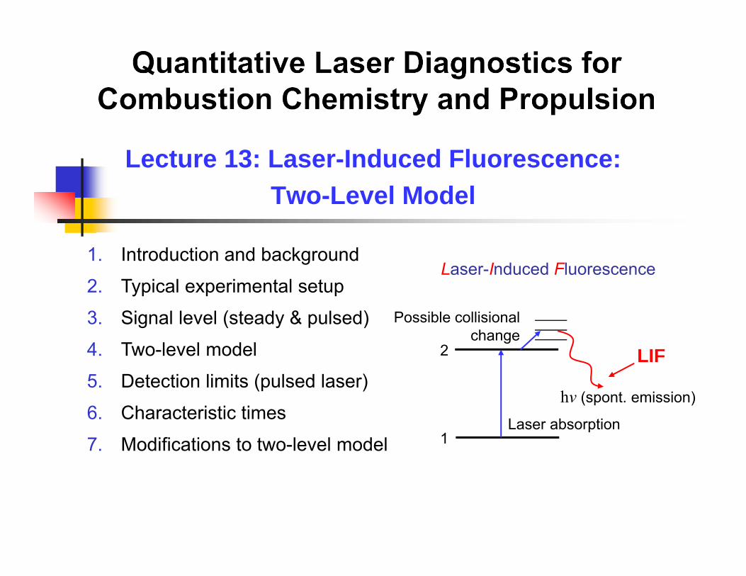
Lecture 13: Laser-Induced Fluorescence:Two-Level Model
1. Introduction and background
2. Typical experimental setup
3. Signal level (steady & pulsed)
4. Two-level model
5. Detection limits (pulsed laser)
6. Characteristic times
7. Modifications to two-level model
Laser-Induced Fluorescence
1
2
Laser absorption
Possible collisionalchange
hν (spont. emission)
LIF
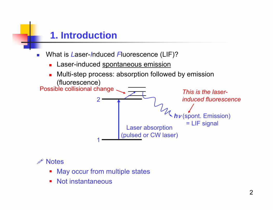
What is Laser-Induced Fluorescence (LIF)? Laser-induced spontaneous emission Multi-step process: absorption followed by emission
(fluorescence)
Notes May occur from multiple states Not instantaneous
2
1. Introduction
2
1
Laser absorption (pulsed or CW laser)
hν (spont. Emission) = LIF signal
This is the laser-induced fluorescence
Possible collisional change
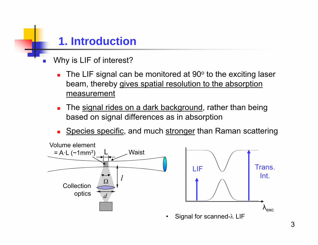
Why is LIF of interest?
The LIF signal can be monitored at 90o to the exciting laser beam, thereby gives spatial resolution to the absorption measurement
The signal rides on a dark background, rather than being based on signal differences as in absorption
Species specific, and much stronger than Raman scattering
3
1. Introduction
Trans. Int.
LIF
λexc
Collection optics
l
d
Ω
Volume element = A·L (~1mm3) L Waist
• Signal for scanned- LIF
4
LIF can be used to monitor multiple gas properties including ni (n,v,J) number density of species i in a state described by n, v, and J T temperature (from the Boltzmann fraction) χi species concentration P pressure (from line broadening) v velocity (from the Doppler shift of the absorption frequency)
And species including Radicals: OH, C2, CN, NH, … Stable diatoms: O2, NO, CO, I2, … Polyatomics: NO2, NCO, CO2, Acetone (CH3COCH3), Biacetyl
((CH3CO)2), Toluene (C7H8), and other carbonyls and aromatic compounds
As well as many atoms….
1. Introduction
1. Introduction
5
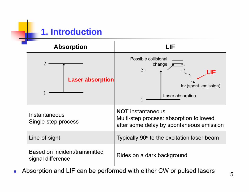
Absorption LIF
InstantaneousSingle-step process
NOT instantaneousMulti-step process: absorption followed after some delay by spontaneous emission
Line-of-sight Typically 90o to the excitation laser beam
Based on incident/transmitted signal difference Rides on a dark background
1
2
Laser absorption
Possible collisionalchange
hν (spont. emission)
LIF
1
2
Laser absorption
Absorption and LIF can be performed with either CW or pulsed lasers
6
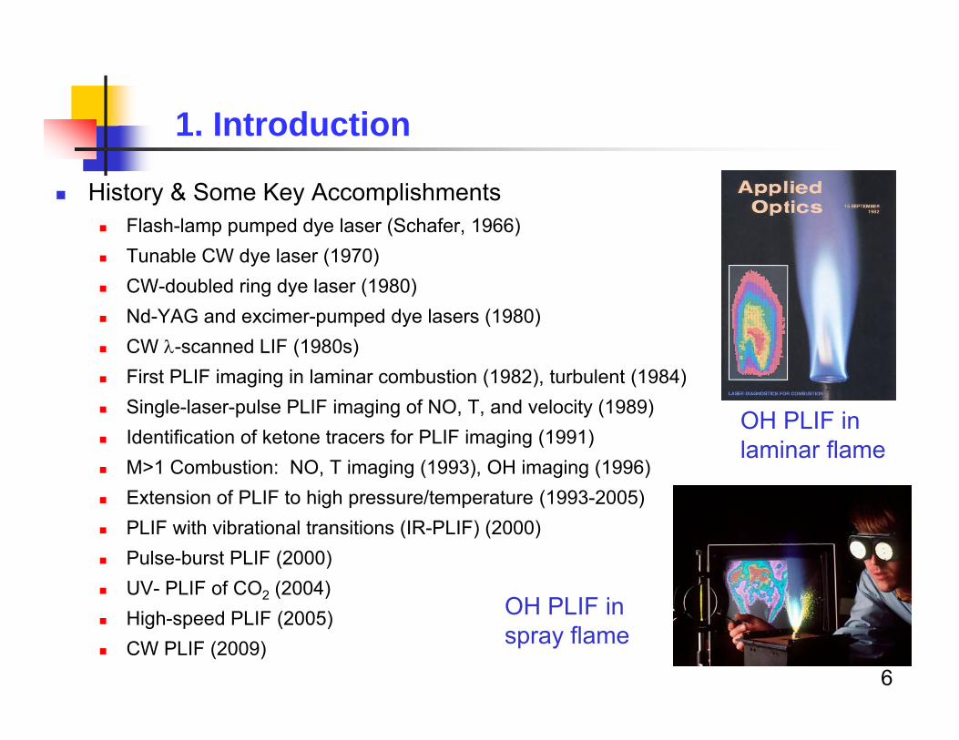
History & Some Key Accomplishments Flash-lamp pumped dye laser (Schafer, 1966) Tunable CW dye laser (1970) CW-doubled ring dye laser (1980) Nd-YAG and excimer-pumped dye lasers (1980) CW -scanned LIF (1980s) First PLIF imaging in laminar combustion (1982), turbulent (1984) Single-laser-pulse PLIF imaging of NO, T, and velocity (1989) Identification of ketone tracers for PLIF imaging (1991) M>1 Combustion: NO, T imaging (1993), OH imaging (1996) Extension of PLIF to high pressure/temperature (1993-2005) PLIF with vibrational transitions (IR-PLIF) (2000) Pulse-burst PLIF (2000) UV- PLIF of CO2 (2004) High-speed PLIF (2005) CW PLIF (2009)
1. Introduction
OH PLIF in spray flame
OH PLIF in laminar flame
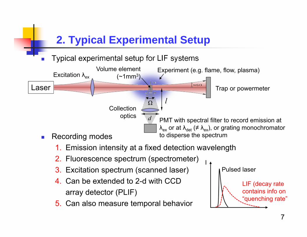
Typical experimental setup for LIF systems
Recording modes1. Emission intensity at a fixed detection wavelength2. Fluorescence spectrum (spectrometer)3. Excitation spectrum (scanned laser)4. Can be extended to 2-d with CCD
array detector (PLIF)5. Can also measure temporal behavior
7
2. Typical Experimental Setup
Experiment (e.g. flame, flow, plasma)
Laser Trap or powermeter
PMT with spectral filter to record emission at λex or at λdet (≠ λex), or grating monochromatorto disperse the spectrum
Collection optics
l
d
Ω
Volume element (~1mm3)Excitation λex
IPulsed laser
LIF (decay rate contains info on “quenching rate”
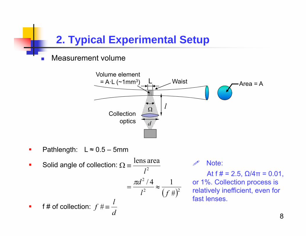
Measurement volume
8
2. Typical Experimental Setup
Pathlength: L ≈ 0.5 – 5mm
Solid angle of collection:
f # of collection:
Area = A
Collection optics
l
d
Ω
Volume element = A·L (~1mm3) L Waist
22
2
2
# 14/
area lens
fldl
dlf #
Note:At f # = 2.5, Ω/4π = 0.01,
or 1%. Collection process is relatively inefficient, even for fast lenses.
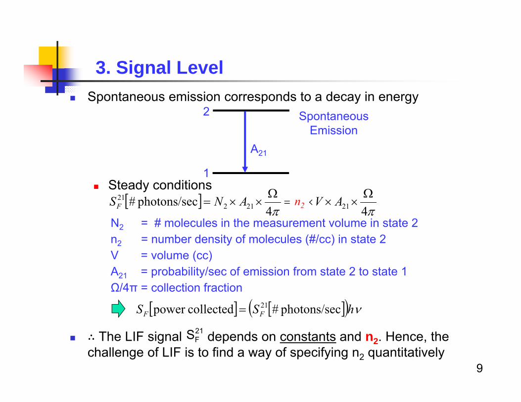
Spontaneous emission corresponds to a decay in energy
Steady conditions
∴ The LIF signal depends on constants and n2. Hence, the challenge of LIF is to find a way of specifying n2 quantitatively
9
3. Signal Level
2
1
A21
Spontaneous Emission
44
cphotons/se # 21221221
AVnANSFN2 = # molecules in the measurement volume in state 2n2 = number density of molecules (#/cc) in state 2V = volume (cc)A21 = probability/sec of emission from state 2 to state 1Ω/4π = collection fraction
hSS FF cphotons/se #collectedpower 21
21FS
n2
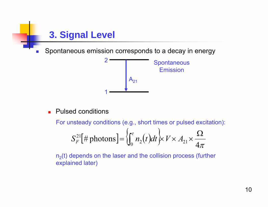
Spontaneous emission corresponds to a decay in energy
Pulsed conditions
10
3. Signal Level
2
1
A21
Spontaneous Emission
For unsteady conditions (e.g., short times or pulsed excitation):
n2(t) depends on the laser and the collision process (further explained later)
4photons # 210 2
21 AVdttnSF
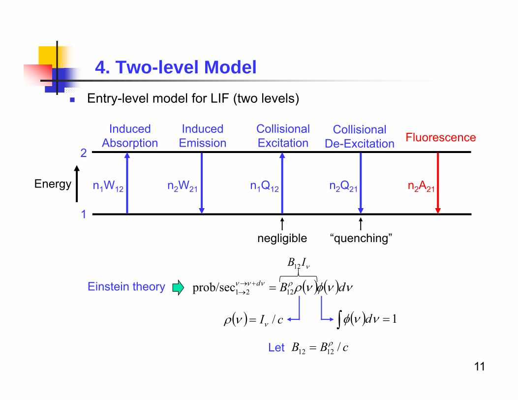
Entry-level model for LIF (two levels)
11
4. Two-level Model
2
1
n1W12
Induced Absorption
dBd1221prob/sec
n2W21 n1Q12 n2Q21 n2A21
Induced Emission
CollisionalExcitation
CollisionalDe-Excitation Fluorescence
Energy
negligible “quenching”
cI / 1 d
Einstein theory
IB12
Let cBB /1212
Entry-level model for LIF (two levels)
12
4. Two-level Model
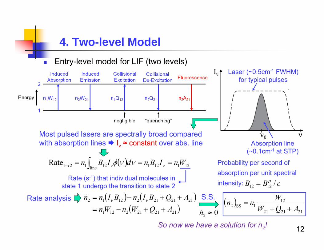
Laser (~0.5cm-1 FWHM) for typical pulses
ν
Iν
Absorption line (~0.1cm-1 at STP)
ν0Most pulsed lasers are spectrally broad compared with absorption lines Iν ≈ constant over abs. line
121121line 12121Rate WnIBndIBn
Rate (s-1) that individual molecules in state 1 undergo the transition to state 2
Probability per second of absorption per unit spectral intensity: cBB /1212
2121212121
21212121212
AQWnWnAQBInBInn
Rate analysis
212121
121SS2 AQW
Wnn
S.S.
02 nSo now we have a solution for n2!
Entry level model for LIF (two levels)
13
4. Two-level Model
212121
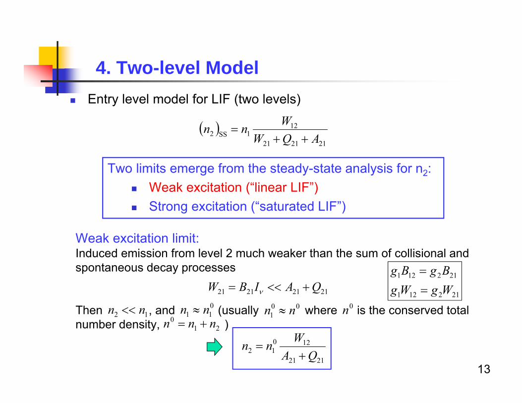
121SS2 AQW
Wnn
Two limits emerge from the steady-state analysis for n2: Weak excitation (“linear LIF”) Strong excitation (“saturated LIF”)
Weak excitation limit:Induced emission from level 2 much weaker than the sum of collisional and spontaneous decay processes
Then , and (usually where is the conserved total number density, )
Two limits emerge from the steady-state analysis for n2: Weak excitation (“linear LIF”) Strong excitation (“saturated LIF”)
21212121 QAIBW
011 nn 12 nn 00
1 nn 0n21
0 nnn
2121
12012 QA
Wnn
212121
212121
WgWgBgBg
Weak excitation limit
14
4. Two-level Model
collectedfraction yield" "fluor.
2121
21
ecabsorbed/s photons
121201
212
4
photons/s 4
QAAIBWVn
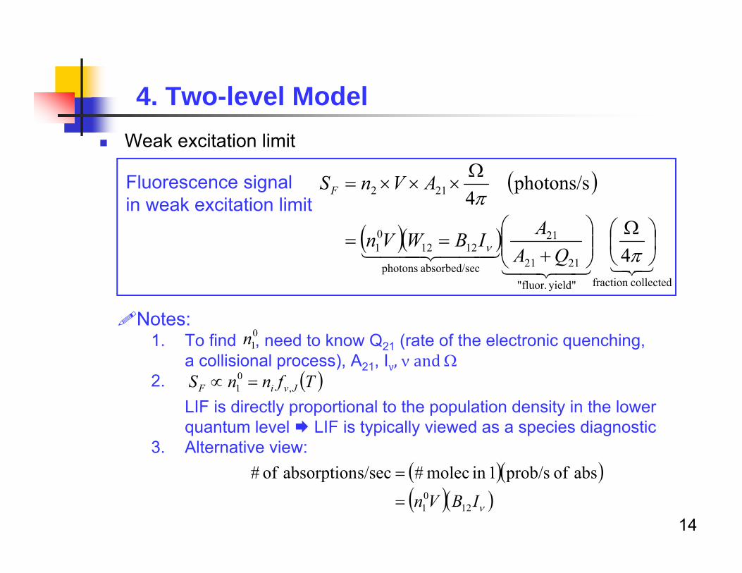
AVnSFFluorescence signalin weak excitation limit
Notes:1. To find , need to know Q21 (rate of the electronic quenching,
a collisional process), A21, Iν, and2.
LIF is directly proportional to the population density in the lower quantum level LIF is typically viewed as a species diagnostic
3. Alternative view:
TfnnS JviF ,01
IBVn 12
01
abs of prob/s1in molec #s/secabsorption of #
01n
Consider the saturation limit
15
4. Two-level Model
Notes:1. If g2 = g1, then n2 = n1, when the transition is “saturated”
2. 12
01
21
01
22101 when
2/1total ggn
ggnnnnn
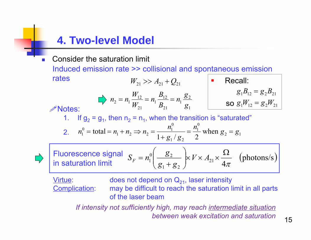
Induced emission rate >> collisional and spontaneous emission rates
212121 QAW
1
21
21
121
21
1212 g
gnBBn
WWnn
Recall:
so 212121
212121
WgWgBgBg
photons/s 421
21
201
AVgg
gnSFFluorescence signalin saturation limit
Virtue: does not depend on Q21, laser intensityComplication: may be difficult to reach the saturation limit in all parts
of the laser beam If intensity not sufficiently high, may reach intermediate situation
between weak excitation and saturation
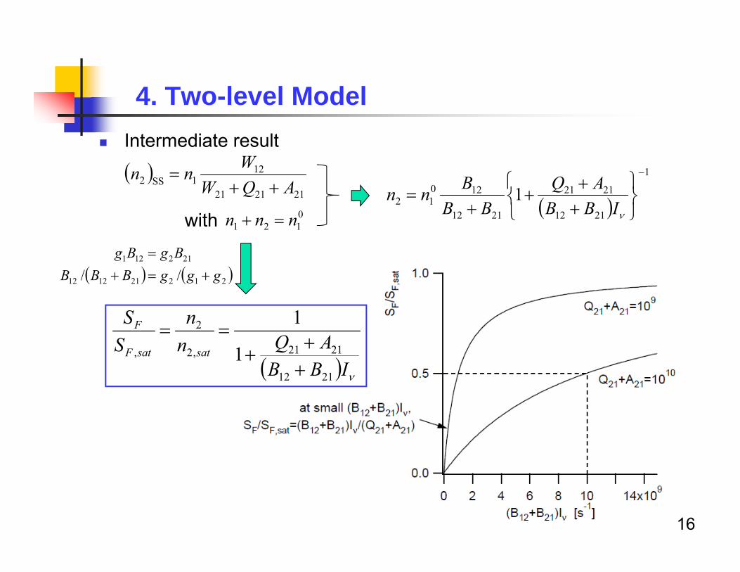
Intermediate result
16
4. Two-level Model
0121 nnn with
1
2112
2121
2112
12012 1
IBB
AQBB
Bnn
212121
121SS2 AQW
Wnn
212211212
212121
// gggBBBBgBg
IBBAQn
nSS
satsatF
F
2112
2121,2
2
, 1
1
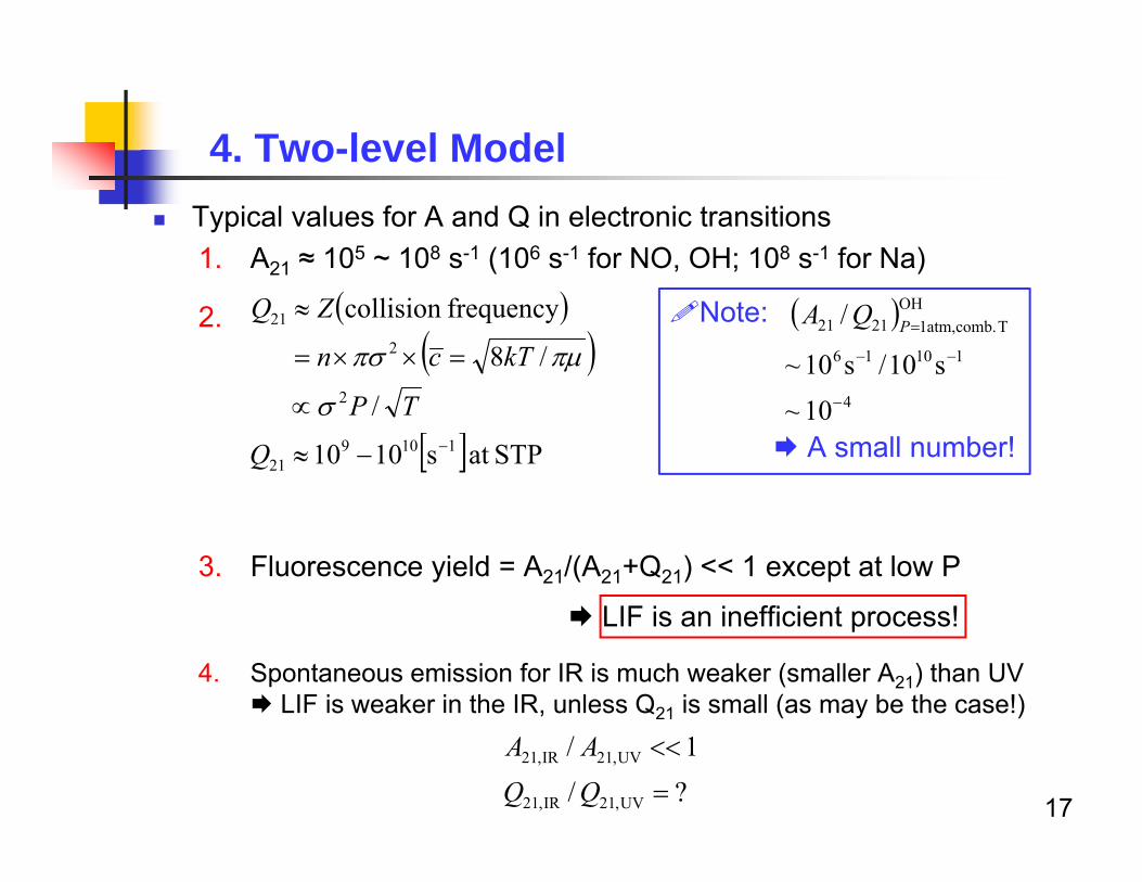
Typical values for A and Q in electronic transitions1. A21 ≈ 105 ~ 108 s-1 (106 s-1 for NO, OH; 108 s-1 for Na)
2.
3. Fluorescence yield = A21/(A21+Q21) << 1 except at low P
LIF is an inefficient process!
4. Spontaneous emission for IR is much weaker (smaller A21) than UV LIF is weaker in the IR, unless Q21 is small (as may be the case!)
17
4. Two-level Model
TP
kTcn
ZQ
/
/8
frequencycollision
2
2
21
STPat s1010 110921
Q
Note:
A small number!
4
11016
OHT comb.atm,12121
10~s10/s10~
/
PQA
?/1/
UV,21IR,21
UV,21IR,21
QQAA
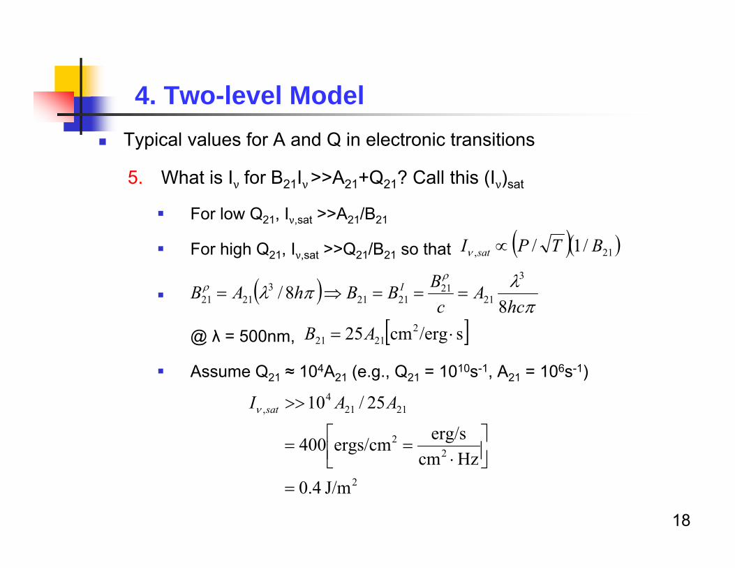
Typical values for A and Q in electronic transitions
5. What is Iν for B21Iν>>A21+Q21? Call this (Iν)sat
For low Q21, Iν,sat >>A21/B21
For high Q21, Iν,sat >>Q21/B21 so that
@ λ = 500nm,
Assume Q21 ≈ 104A21 (e.g., Q21 = 1010s-1, A21 = 106s-1)
18
4. Two-level Model
21, /1/ BTPI sat
hcA
cBBBhAB I
88/
3
2121
21213
2121
s/ergcm25 22121 AB
2
22
21214
,
J/m4.0Hzcm
erg/sergs/cm400
25/10
AAI sat
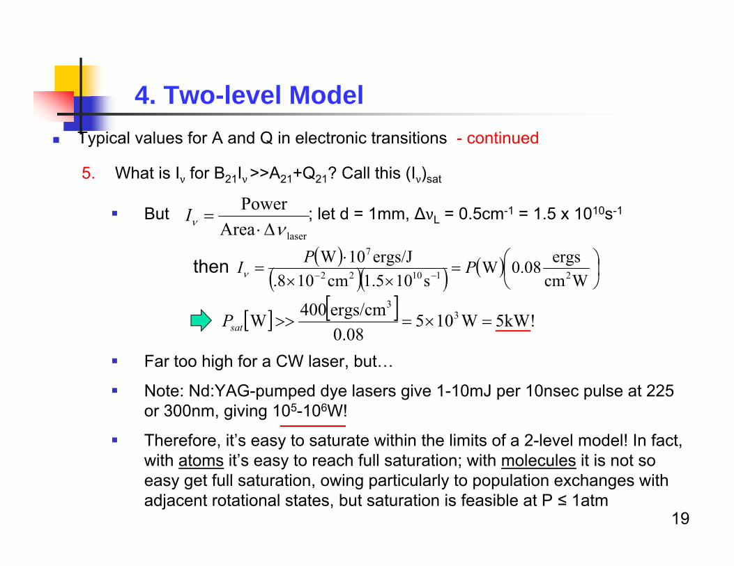
Typical values for A and Q in electronic transitions - continued
5. What is Iν for B21Iν>>A21+Q21? Call this (Iν)sat
But ; let d = 1mm, ∆νL = 0.5cm-1 = 1.5 x 10¹⁰s-1
Far too high for a CW laser, but…
Note: Nd:YAG-pumped dye lasers give 1-10mJ per 10nsec pulse at 225 or 300nm, giving 105-106W!
Therefore, it’s easy to saturate within the limits of a 2-level model! In fact, with atoms it’s easy to reach full saturation; with molecules it is not so easy get full saturation, owing particularly to population exchanges with adjacent rotational states, but saturation is feasible at P ≤ 1atm
19
4. Two-level Model
laserAreaPower
I
5kW!W1050.08ergs/cm400W 3
3
satP
then
Wcmergs08.0W
s105.1cm108.ergs/J10W
211022
7
PPI
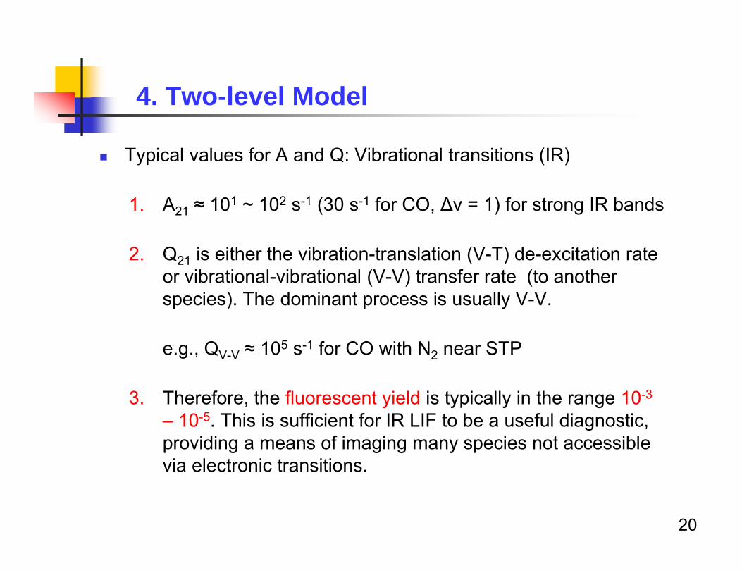
Typical values for A and Q: Vibrational transitions (IR)
1. A21 ≈ 101 ~ 102 s-1 (30 s-1 for CO, ∆v = 1) for strong IR bands
2. Q21 is either the vibration-translation (V-T) de-excitation rate or vibrational-vibrational (V-V) transfer rate (to another species). The dominant process is usually V-V.
e.g., QV-V ≈ 105 s-1 for CO with N2 near STP
3. Therefore, the fluorescent yield is typically in the range 10-3
– 10-5. This is sufficient for IR LIF to be a useful diagnostic, providing a means of imaging many species not accessible via electronic transitions.
20
4. Two-level Model
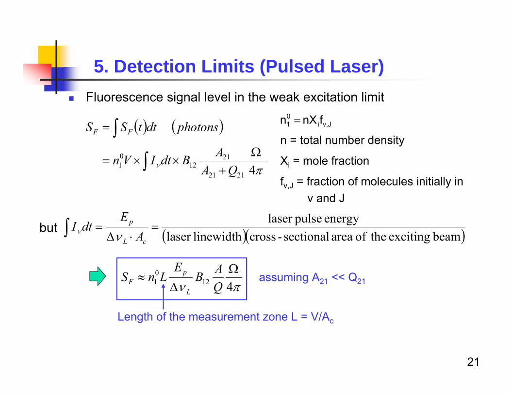
Fluorescence signal level in the weak excitation limit
21
5. Detection Limits (Pulsed Laser)
42121
2112
01
QAABdtIVn
photonsdttSS FFJv,i
01 fnXn
n = total number density
Xi = mole fraction
fv,J = fraction of molecules initially in v and J
beam exciting theof area sectional-crosslinewidthlaser energy pulselaser
cL
p
AE
dtI
41201
QAB
ELnS
L
pF
Length of the measurement zone L = V/Ac
assuming A21 << Q21
but
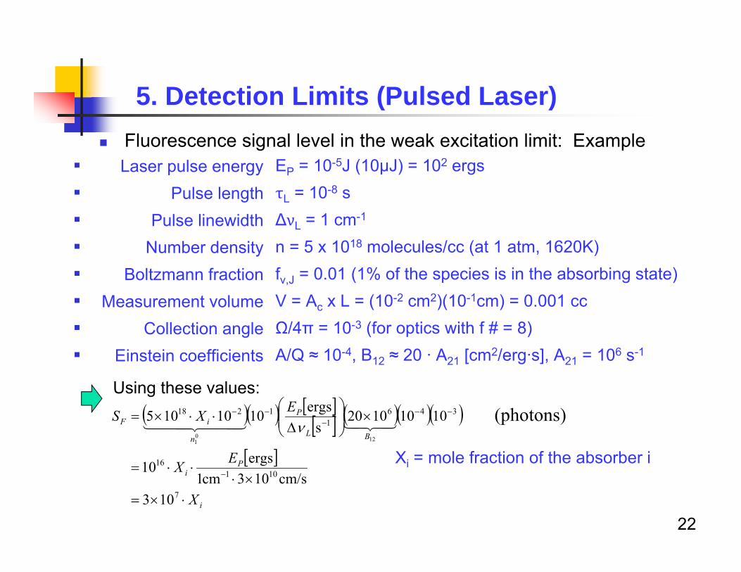
Fluorescence signal level in the weak excitation limit: Example
22
5. Detection Limits (Pulsed Laser)
EP = 10-5J (10μJ) = 102 ergs τL = 10-8 s ∆νL = 1 cm-1
n = 5 x 10¹⁸ molecules/cc (at 1 atm, 1620K) fv,J = 0.01 (1% of the species is in the absorbing state) V = Ac x L = (10-2 cm2)(10-1cm) = 0.001 cc Ω/4π = 10-3 (for optics with f # = 8) A/Q ≈ 10-4, B12 ≈ 20 · A21 [cm2/erg·s], A21 = 106 s-1
Laser pulse energyPulse length
Pulse linewidthNumber density
Boltzmann fractionMeasurement volume
Collection angleEinstein coefficients
i
Pi
BL
P
n
iF
X
EX
EXS
7
10116
3461
1218
103cm/s103cm1
ergs10
10101020s
ergs1010105120
1
Xi = mole fraction of the absorber i
Using these values:(photons)
Fluorescence signal level in the weak excitation limit: Example
23
5. Detection Limits (Pulsed Laser)
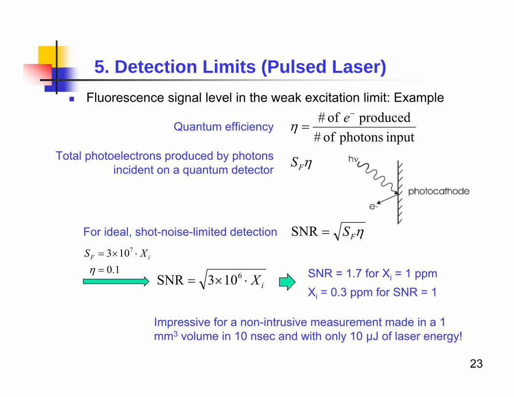
Quantum efficiency
Total photoelectrons produced by photons incident on a quantum detector
input photons of #produced of #
e
FS
For ideal, shot-noise-limited detection FSSNR
1.0103 7
iF XS
iX 6103SNR SNR = 1.7 for Xi = 1 ppmXi = 0.3 ppm for SNR = 1
Impressive for a non-intrusive measurement made in a 1 mm3 volume in 10 nsec and with only 10 μJ of laser energy!
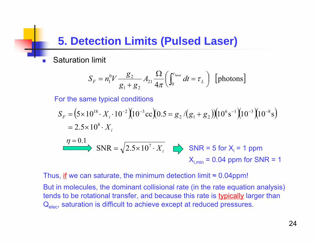
Saturation limit
24
5. Detection Limits (Pulsed Laser)
photons 4
laser
02121
201
LF dtAgg
gVnS
For the same typical conditions
i
iF
X
gggXS
8
8316212
3218
105.2
s1010s10/5.0cc1010105
iX 7105.2SNR1.0
SNR = 5 for Xi = 1 ppmXi,min = 0.04 ppm for SNR = 1
Thus, if we can saturate, the minimum detection limit ≈ 0.04ppm!But in molecules, the dominant collisional rate (in the rate equation analysis) tends to be rotational transfer, and because this rate is typically larger than Qelec, saturation is difficult to achieve except at reduced pressures.
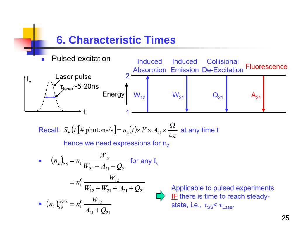
Pulsed excitation
25
6. Characteristic Times
2
1
W12
Induced Absorption
W21 Q21 A21
Induced Emission
CollisionalDe-Excitation Fluorescence
Energy
Laser pulseτlaser~5-20ns
t
Iν
Recall: at any time t
hence we need expressions for n2
for any Iν
2121
1201
weakSS2
21212112
1201
212121
121SS2
QAWnn
QAWWWn
QAWWnn
Applicable to pulsed experiments IF there is time to reach steady-state, i.e., τSS< τLaser
4
photons/s # 212
AVtntSF
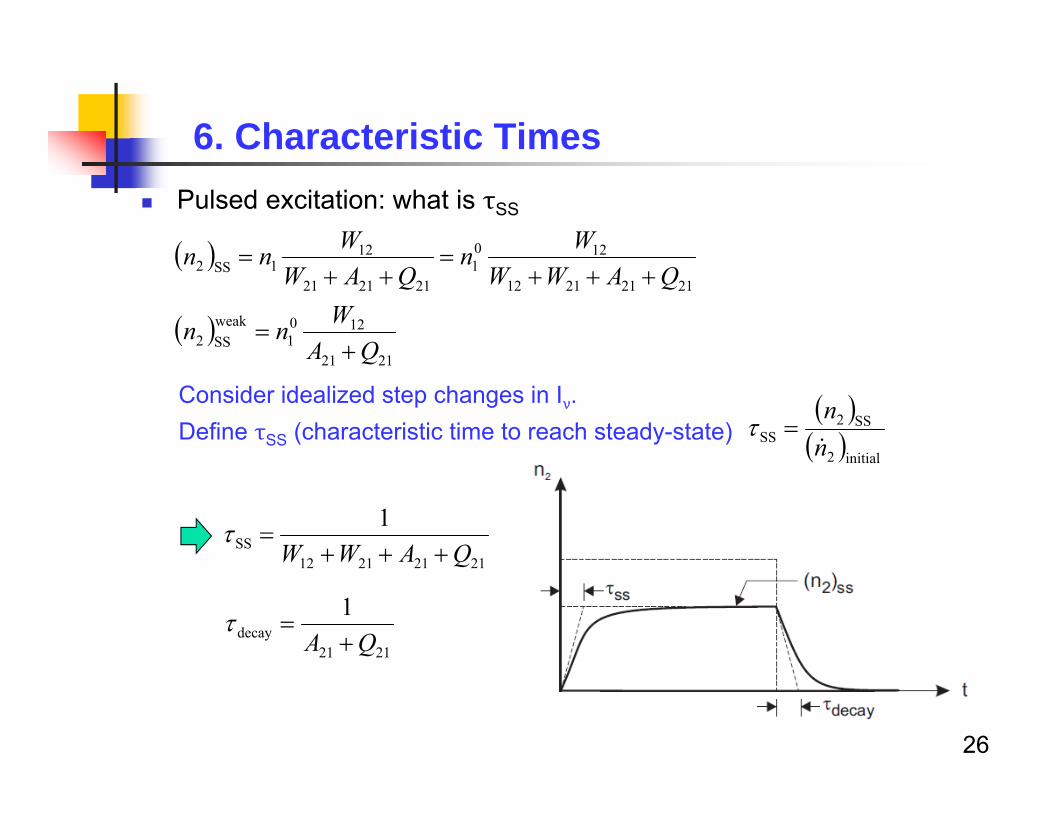
Pulsed excitation: what is τSS
26
6. Characteristic Times
2121
1201
weakSS2
21212112
1201
212121
121SS2
QAWnn
QAWWWn
QAWWnn
Consider idealized step changes in Iν.Define τSS (characteristic time to reach steady-state)
initial2
SS2SS n
n
21212112SS
1QAWW
2121decay
1QA
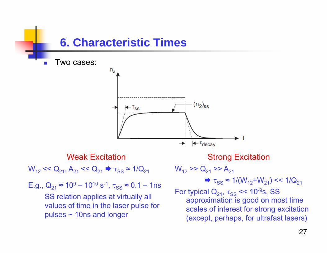
Two cases:
27
6. Characteristic Times
Weak ExcitationW12 << Q21, A21 << Q21 τSS ≈ 1/Q21
E.g., Q21 ≈ 109 – 1010 s-1, τSS ≈ 0.1 – 1nsSS relation applies at virtually all values of time in the laser pulse for pulses ~ 10ns and longer
Strong ExcitationW12 >> Q21 >> A21
τSS ≈ 1/(W12+W21) << 1/Q21
For typical Q21, τSS << 10-9s, SSapproximation is good on most time scales of interest for strong excitation (except, perhaps, for ultrafast lasers)
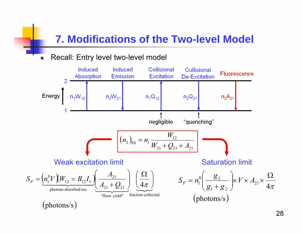
Recall: Entry level two-level model
28
7. Modifications of the Two-level Model
Weak excitation limit
212121
121SS2 AQW
Wnn
photons/s
4collectedfraction yield" "fluor.
2121
21
ecabsorbed/s photons
121201
QA
AIBWVnSF
photons/s 421
21
201
AVgg
gnSF
Saturation limit
Hole-burning effects
Multi-level effects
29
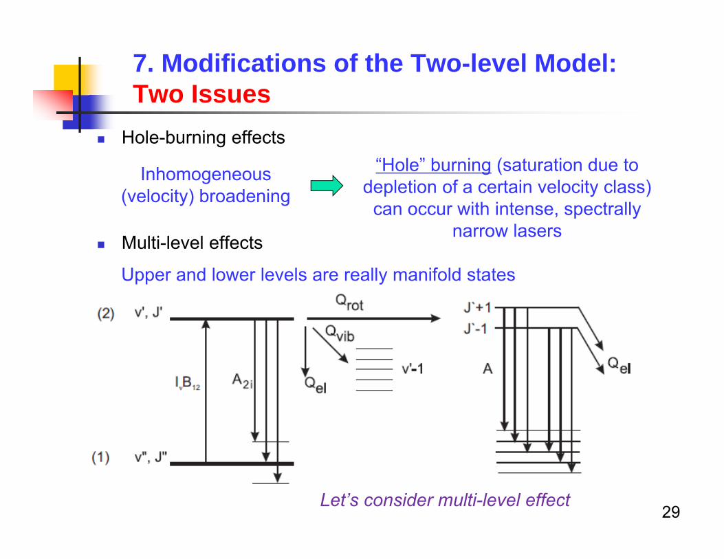
7. Modifications of the Two-level Model: Two Issues
Inhomogeneous (velocity) broadening
“Hole” burning (saturation due to depletion of a certain velocity class)
can occur with intense, spectrally narrow lasers
Upper and lower levels are really manifold states
Let’s consider multi-level effect
Multi-level effects
Narrowband detection: emission is collected only from v', J'
30
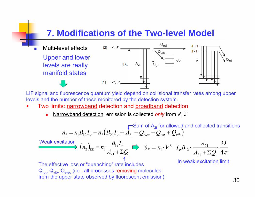
7. Modifications of the Two-level Model
Upper and lower levels are really manifold states
LIF signal and fluorescence quantum yield depend on collisional transfer rates among upper levels and the number of these monitored by the detection system. Two limits: narrowband detection and broadband detection
vibrotelec QQQAIBnIBnn 212121212 Sum of A2i for allowed and collected transitions
Weak excitation
421
2112
01
QAABIVnSF
In weak excitation limit
QA
IBnn
21
121SS2
The effective loss or “quenching” rate includesQrot, Qvib, Qelec (i.e., all processes removing molecules from the upper state observed by fluorescent emission)
Multi-level effects
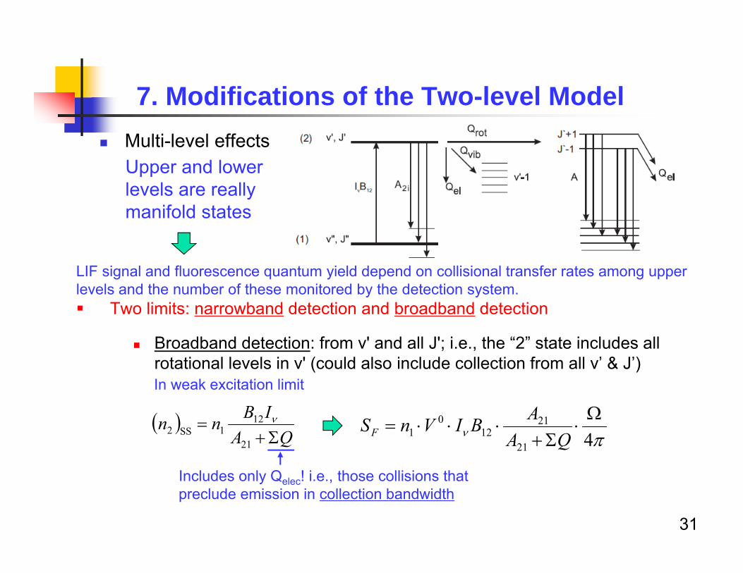
Broadband detection: from v' and all J'; i.e., the “2” state includes all rotational levels in v' (could also include collection from all v’ & J’)
31
7. Modifications of the Two-level Model
Upper and lower levels are really manifold states
LIF signal and fluorescence quantum yield depend on collisional transfer rates among upper levels and the number of these monitored by the detection system. Two limits: narrowband detection and broadband detection
421
2112
01
QAABIVnSF
QAIBnn
21
121SS2
Includes only Qelec! i.e., those collisions that preclude emission in collection bandwidth
In weak excitation limit
Multi-level effects
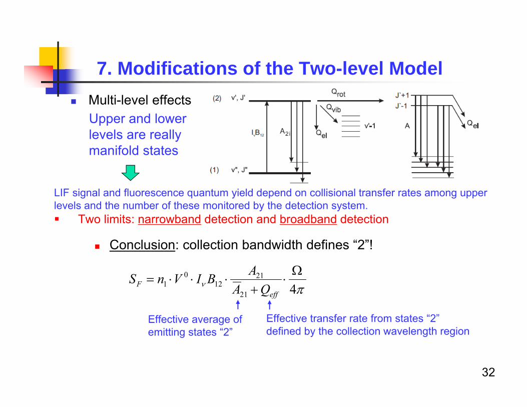
Conclusion: collection bandwidth defines “2”!
32
7. Modifications of the Two-level Model
Upper and lower levels are really manifold states
LIF signal and fluorescence quantum yield depend on collisional transfer rates among upper levels and the number of these monitored by the detection system. Two limits: narrowband detection and broadband detection
421
2112
01
effF QA
ABIVnS
Effective average of emitting states “2”
Effective transfer rate from states “2” defined by the collection wavelength region
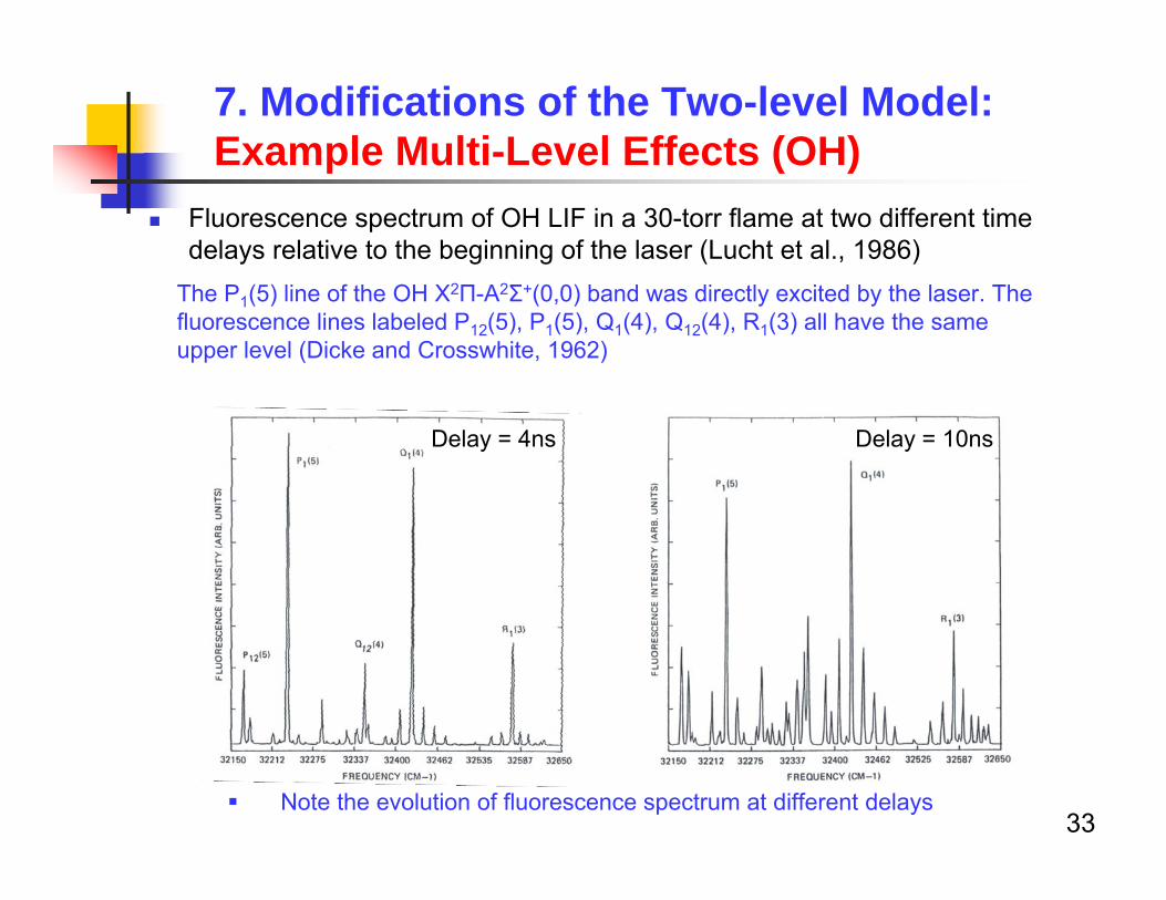
Fluorescence spectrum of OH LIF in a 30-torr flame at two different time delays relative to the beginning of the laser (Lucht et al., 1986)
33
7. Modifications of the Two-level Model: Example Multi-Level Effects (OH)
The P1(5) line of the OH X2Π-A2Σ+(0,0) band was directly excited by the laser. The fluorescence lines labeled P12(5), P1(5), Q1(4), Q12(4), R1(3) all have the same upper level (Dicke and Crosswhite, 1962)
Note the evolution of fluorescence spectrum at different delays
Delay = 4ns Delay = 10ns
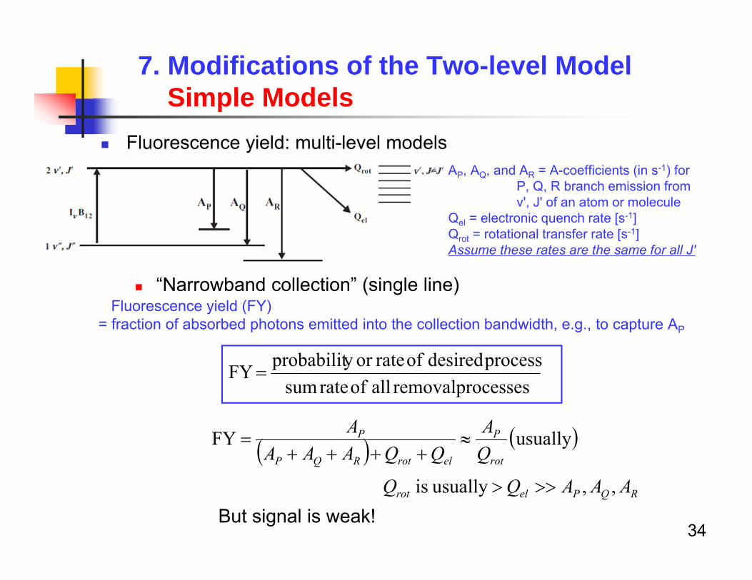
Fluorescence yield: multi-level models
“Narrowband collection” (single line)
34
7. Modifications of the Two-level ModelSimple Models
AP, AQ, and AR = A-coefficients (in s-1) for P, Q, R branch emission from v', J' of an atom or molecule
Qel = electronic quench rate [s-1]Qrot = rotational transfer rate [s-1]Assume these rates are the same for all J'
Fluorescence yield (FY)= fraction of absorbed photons emitted into the collection bandwidth, e.g., to capture AP
processes removal all of rate sumprocess desired of rateor y probabilitFY
usuallyFYrot
P
elrotRQP
P
QA
QQAAAA
RQPelrot AAAQQ ,,usually is
But signal is weak!
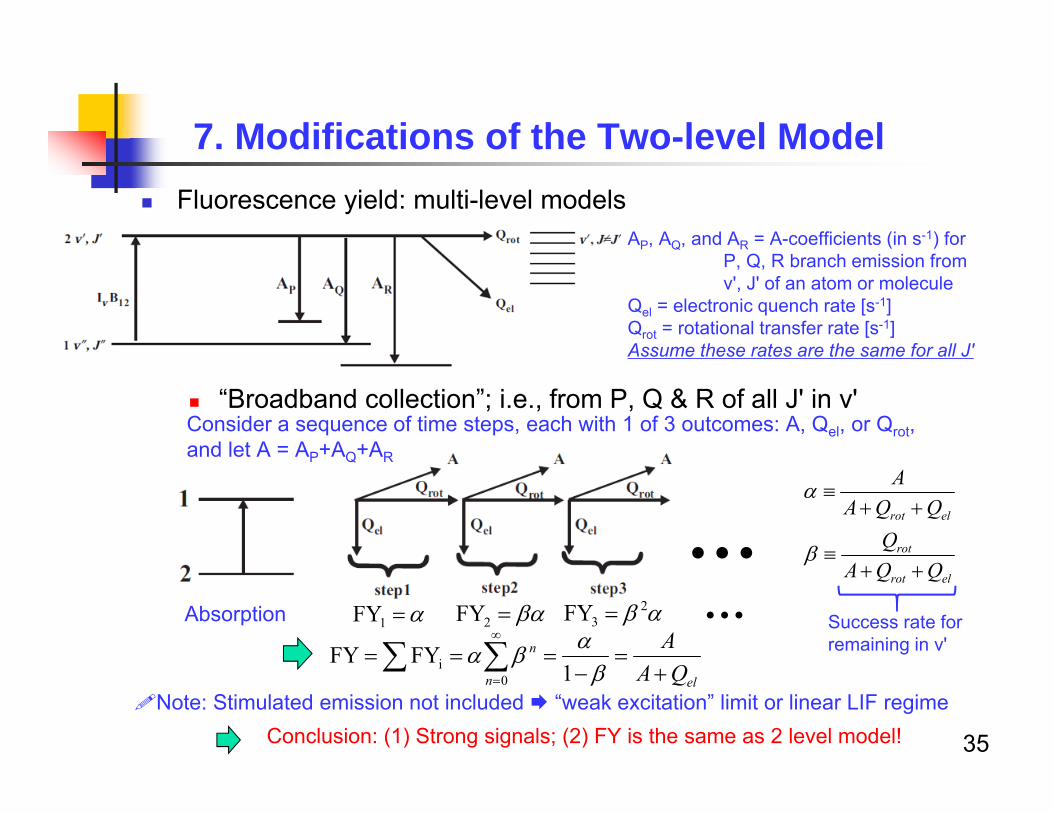
Fluorescence yield: multi-level models
“Broadband collection”; i.e., from P, Q & R of all J' in v'
35
7. Modifications of the Two-level Model
AP, AQ, and AR = A-coefficients (in s-1) for P, Q, R branch emission from v', J' of an atom or molecule
Qel = electronic quench rate [s-1]Qrot = rotational transfer rate [s-1]Assume these rates are the same for all J'
Note: Stimulated emission not included “weak excitation” limit or linear LIF regime
1FY
elrot
rot
elrot
QQAQ
QQAA
…Absorption 2FY 2
3FY …eln
n
QAA
1FYFY
0i
Consider a sequence of time steps, each with 1 of 3 outcomes: A, Qel, or Qrot, and let A = AP+AQ+AR
Success rate for remaining in v'
Conclusion: (1) Strong signals; (2) FY is the same as 2 level model!
Next Lecture – LIF/PLIF of Small Molecules
LIF is spatially-resolved with signal from a point or a line Excite LIF with the laser expanded into a narrow sheet and
collect the fluorescence with a camera :Planar Laser-Induced Fluorescence or PLIF
Applications of PLIF to small (diatomic) radicals (e.g., OH & NO)
36