Embed Size (px)
Citation preview
Lecture 18 Molecular Evolution and Phylogenetics
6.047/6.878 - Computational Biology: Genomes, Networks, Evolution
Somewhere, something went wrong…
Pat
rick
Win
ston
’s 6
.034
1
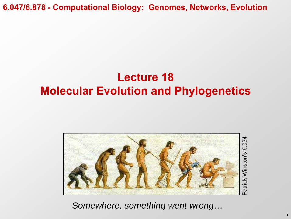
Challenges in Computational Biology
DNA
4 Genome Assembly
1 Gene Finding 5 Regulatory motif discovery
Database lookup 3
Gene expression analysis 8
RNA transcript
Sequence alignment 2
Evolutionary Theory 7 TCATGCTAT TCGTGATAA TGAGGATAT TTATCATAT TTATGATTT
Cluster discovery 9 Gibbs sampling 10
Protein network analysis 11
12 Metabolic modelling
Comparative Genomics 6
Emerging network properties 13
2
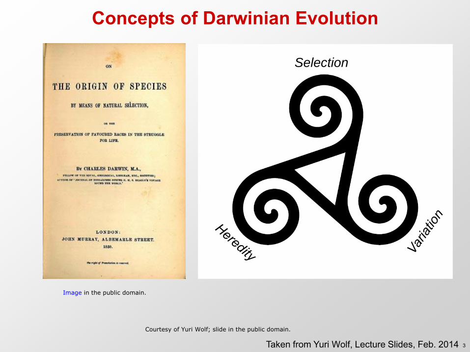
Concepts of Darwinian Evolution
Selection
Taken from Yuri Wolf, Lecture Slides, Feb. 2014
Image in the public domain.
Courtesy of Yuri Wolf; slide in the public domain.
3
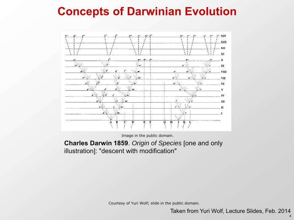
Concepts of Darwinian Evolution
Charles Darwin 1859. Origin of Species [one and only illustration]: "descent with modification"
Taken from Yuri Wolf, Lecture Slides, Feb. 2014
Image in the public domain.
Courtesy of Yuri Wolf; slide in the public domain.
4
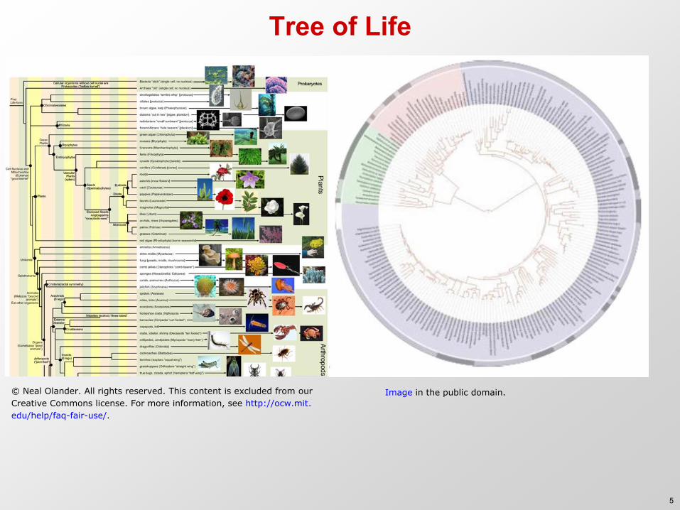
Tree of Life
Image in the public domain.© Neal Olander. All rights reserved. This content is excluded from our
Creative Commons license. For more information, see http://ocw.mit.
edu/help/faq-fair-use/.
5
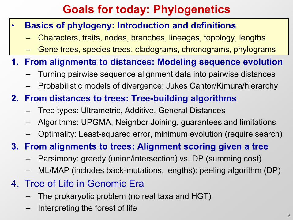
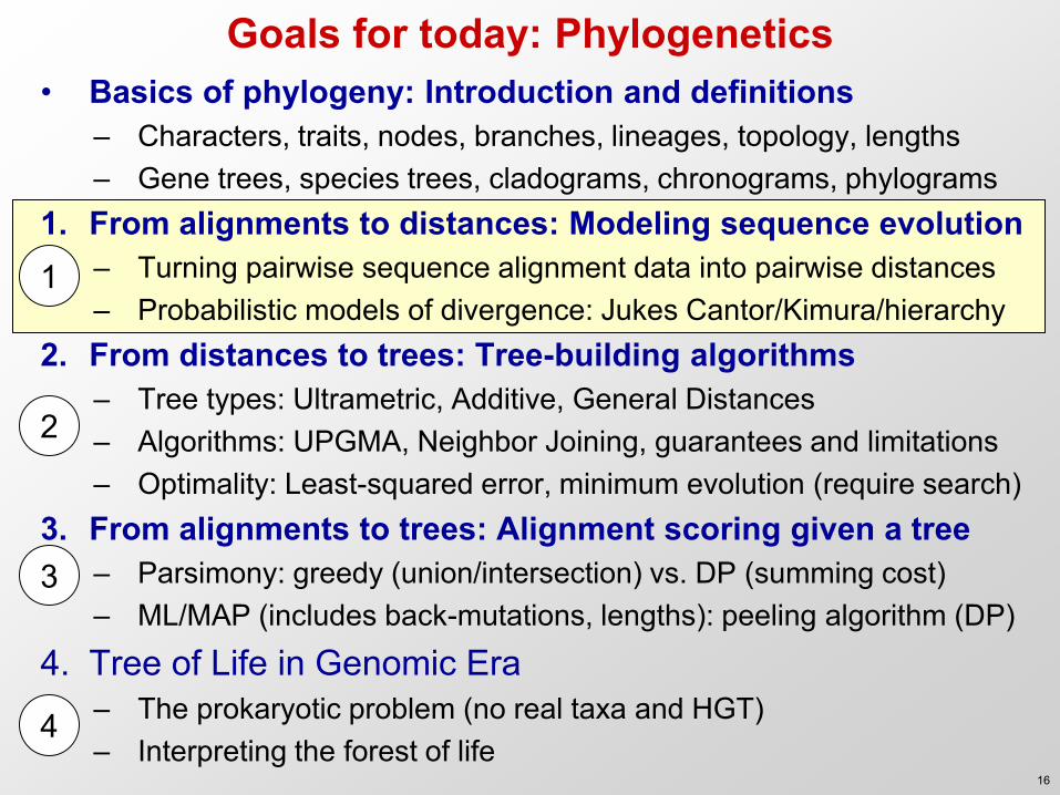
Goals for today: Phylogenetics • Basics of phylogeny: Introduction and definitions
– Characters, traits, nodes, branches, lineages, topology, lengths – Gene trees, species trees, cladograms, chronograms, phylograms
1. From alignments to distances: Modeling sequence evolution – Turning pairwise sequence alignment data into pairwise distances – Probabilistic models of divergence: Jukes Cantor/Kimura/hierarchy
2. From distances to trees: Tree-building algorithms – Tree types: Ultrametric, Additive, General Distances – Algorithms: UPGMA, Neighbor Joining, guarantees and limitations – Optimality: Least-squared error, minimum evolution (require search)
3. From alignments to trees: Alignment scoring given a tree – Parsimony: greedy (union/intersection) vs. DP (summing cost) – ML/MAP (includes back-mutations, lengths): peeling algorithm (DP)
4. Tree of Life in Genomic Era – The prokaryotic problem (no real taxa and HGT) – Interpreting the forest of life
6
Introduction: Basics and Definitions
Characters, traits, gene/species trees
7
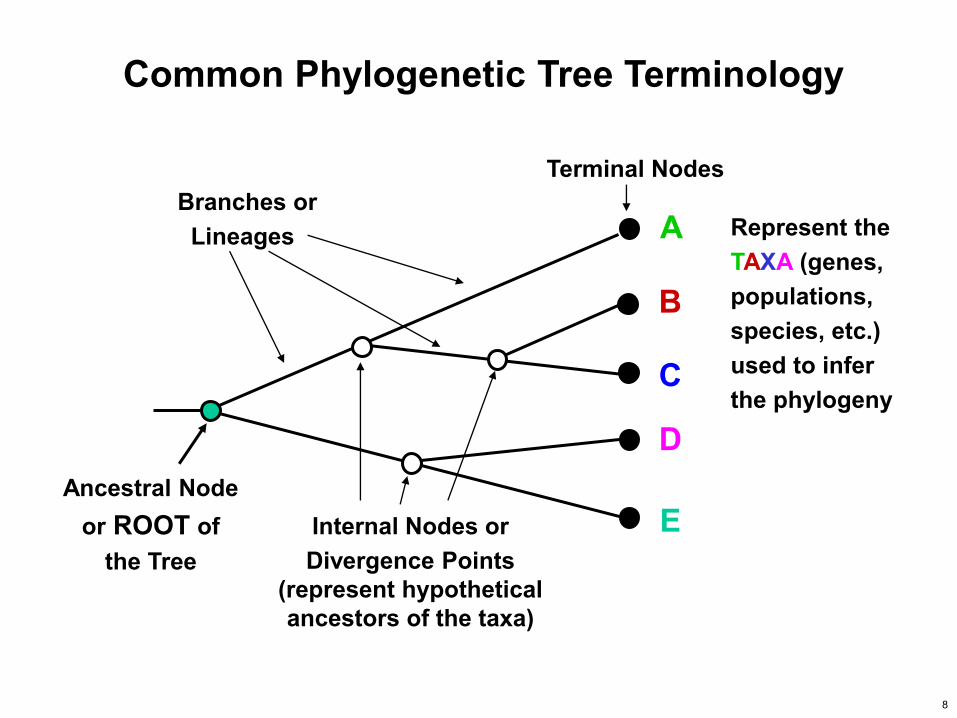
Ancestral Node or ROOT of
the Tree Internal Nodes or Divergence Points
(represent hypothetical ancestors of the taxa)
Branches or Lineages
Terminal Nodes
A
B
C
D
E
Represent the TAXA (genes, populations, species, etc.) used to infer the phylogeny
Common Phylogenetic Tree Terminology
8

Extinctions part of life
Phylogenetic tree showing archosaurs, dinosaurs, birds, etc. through geologic time removed due to copyright restrictions.
9
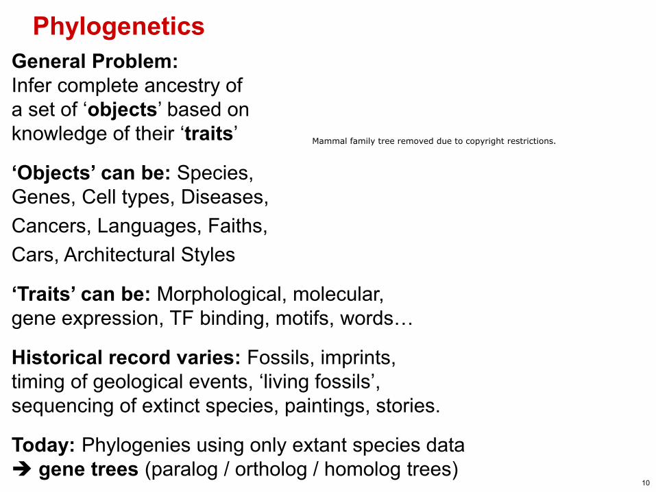
Phylogenetics General Problem: Infer complete ancestry of a set of ‘objects’ based on knowledge of their ‘traits’
‘Objects’ can be: Species, Genes, Cell types, Diseases, Cancers, Languages, Faiths, Cars, Architectural Styles
‘Traits’ can be: Morphological, molecular, gene expression, TF binding, motifs, words…
Historical record varies: Fossils, imprints, timing of geological events, ‘living fossils’, sequencing of extinct species, paintings, stories.
Today: Phylogenies using only extant species data gene trees (paralog / ortholog / homolog trees)
Mammal family tree removed due to copyright restrictions.
10
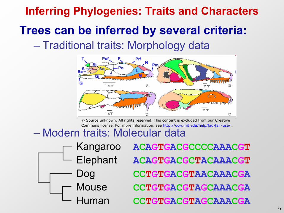
Inferring Phylogenies: Traits and Characters
Trees can be inferred by several criteria: – Traditional traits: Morphology data
– Modern traits: Molecular data Kangaroo ACAGTGACGCCCCAAACGT Elephant ACAGTGACGCTACAAACGT Dog CCTGTGACGTAACAAACGA Mouse CCTGTGACGTAGCAAACGA Human CCTGTGACGTAGCAAACGA
© Source unknown. All rights reserved. This content is excluded from our Creative
Commons license. For more information, see http://ocw.mit.edu/help/faq-fair-use/.
11
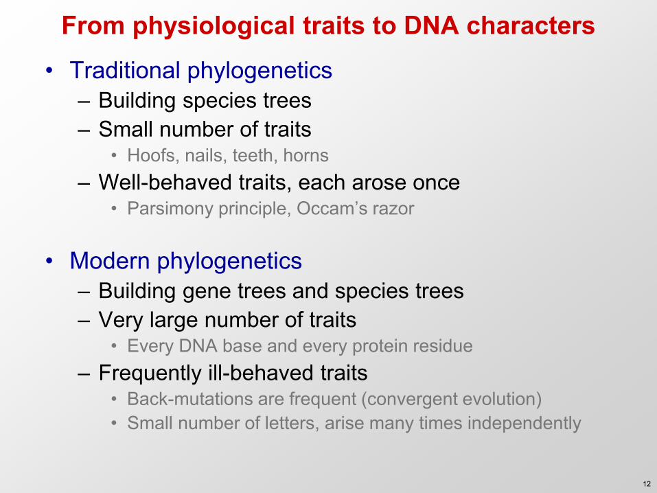
From physiological traits to DNA characters • Traditional phylogenetics
– Building species trees – Small number of traits
• Hoofs, nails, teeth, horns – Well-behaved traits, each arose once
• Parsimony principle, Occam’s razor
• Modern phylogenetics – Building gene trees and species trees – Very large number of traits
• Every DNA base and every protein residue – Frequently ill-behaved traits
• Back-mutations are frequent (convergent evolution) • Small number of letters, arise many times independently
12
Taxon A
Taxon B
Taxon C
Taxon D
1 1
1
6
3
5
Taxon A
Taxon B
Taxon C
Taxon D
Taxon A
Taxon B
Taxon C
Taxon D
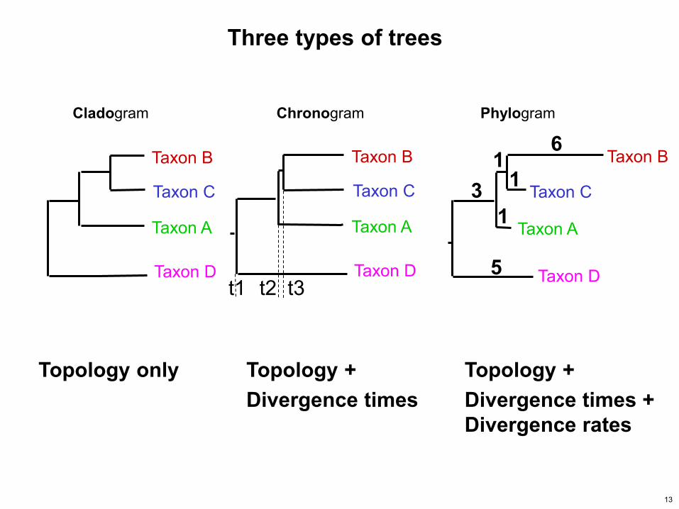
Three types of trees
Cladogram Chronogram Phylogram
Topology only Topology + Divergence times
Topology + Divergence times + Divergence rates
t1 t3 t2
13
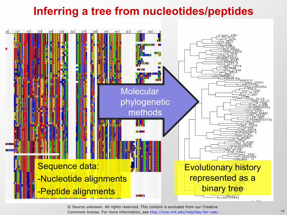
Inferring a tree from nucleotides/peptides
Molecular phylogenetic
methods
Sequence data: -Nucleotide alignments -Peptide alignments
Evolutionary history represented as a
binary tree
© Source unknown. All rights reserved. This content is excluded from our Creative
Commons license. For more information, see http://ocw.mit.edu/help/faq-fair-use/. 14
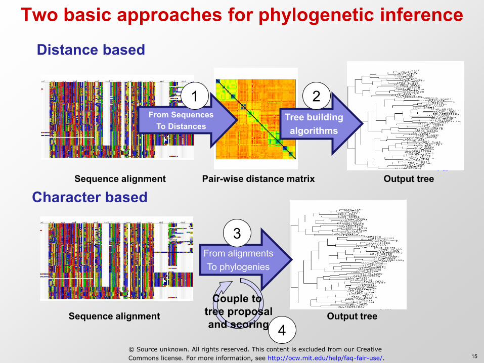
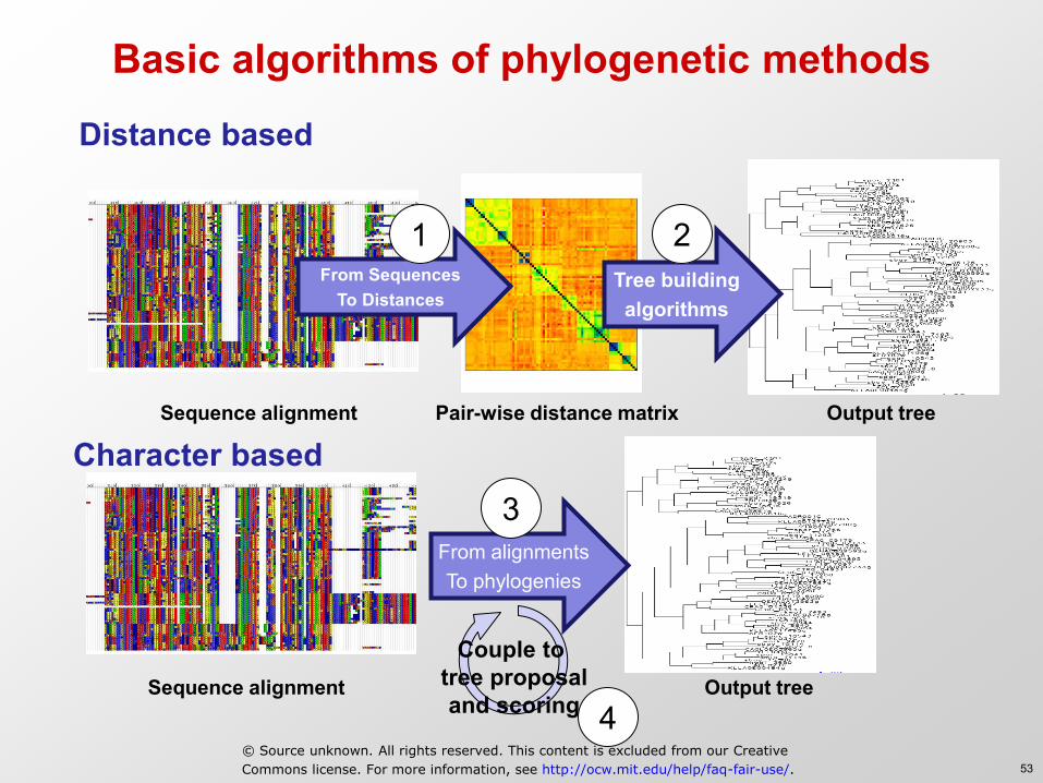
Two basic approaches for phylogenetic inference
Distance based
Character based
From alignments To phylogenies
From Sequences To Distances
Tree building algorithms
Pair-wise distance matrix Sequence alignment
Sequence alignment Output tree
Output tree
Couple to tree proposal and scoring
1 2
3
4 15
© Source unknown. All rights reserved. This content is excluded from our Creative
Commons license. For more information, see http://ocw.mit.edu/help/faq-fair-use/.
Goals for today: Phylogenetics • Basics of phylogeny: Introduction and definitions
– Characters, traits, nodes, branches, lineages, topology, lengths – Gene trees, species trees, cladograms, chronograms, phylograms
1. From alignments to distances: Modeling sequence evolution – Turning pairwise sequence alignment data into pairwise distances – Probabilistic models of divergence: Jukes Cantor/Kimura/hierarchy
2. From distances to trees: Tree-building algorithms – Tree types: Ultrametric, Additive, General Distances – Algorithms: UPGMA, Neighbor Joining, guarantees and limitations – Optimality: Least-squared error, minimum evolution (require search)
3. From alignments to trees: Alignment scoring given a tree – Parsimony: greedy (union/intersection) vs. DP (summing cost) – ML/MAP (includes back-mutations, lengths): peeling algorithm (DP)
4. Tree of Life in Genomic Era – The prokaryotic problem (no real taxa and HGT) – Interpreting the forest of life
1
2
3
4 16
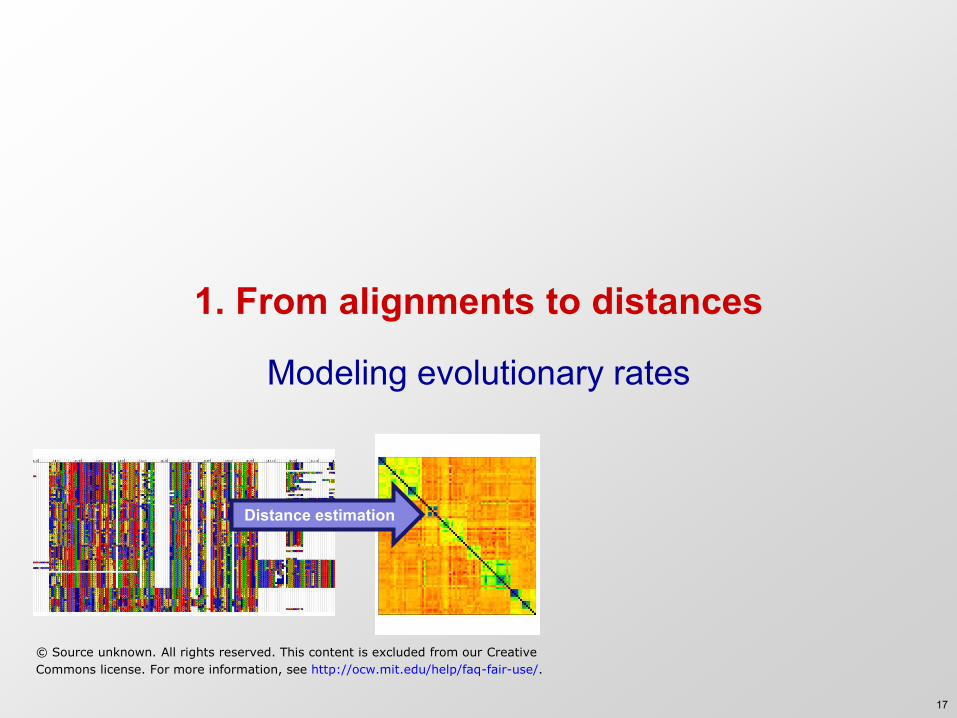
1. From alignments to distances
Modeling evolutionary rates
Distance estimation
17
© Source unknown. All rights reserved. This content is excluded from our Creative
Commons license. For more information, see http://ocw.mit.edu/help/faq-fair-use/.
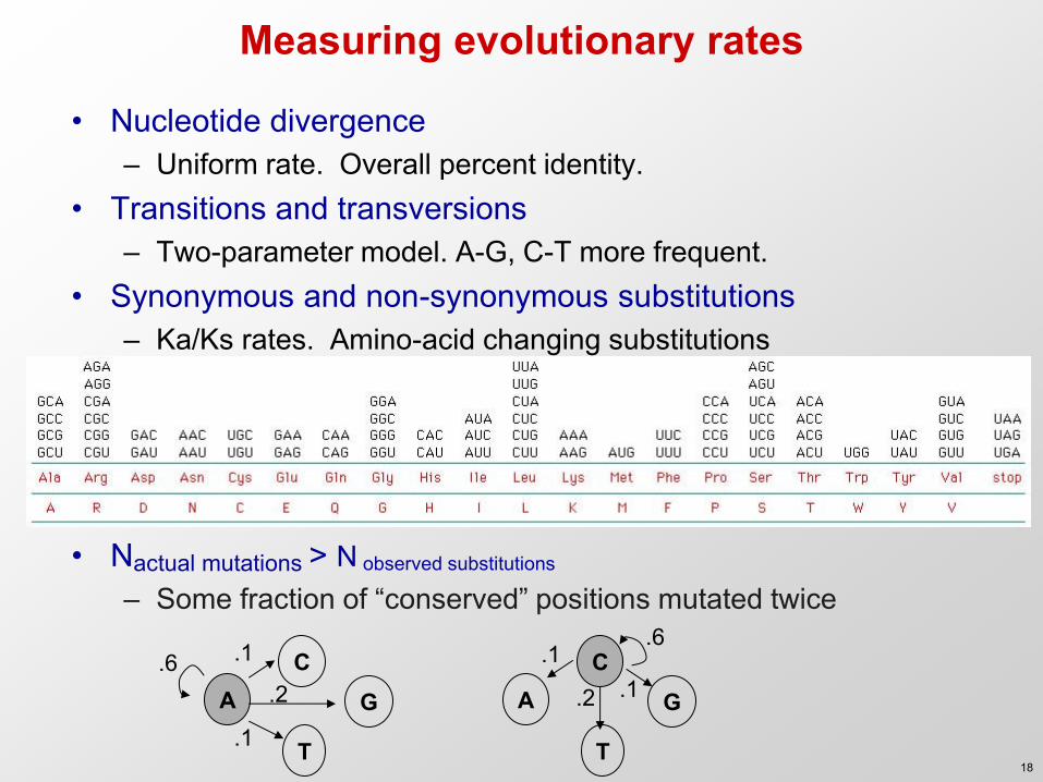
Measuring evolutionary rates
• Nucleotide divergence – Uniform rate. Overall percent identity.
• Transitions and transversions – Two-parameter model. A-G, C-T more frequent.
• Synonymous and non-synonymous substitutions – Ka/Ks rates. Amino-acid changing substitutions
• Nactual mutations > N observed substitutions – Some fraction of “conserved” positions mutated twice
A C
G
T
A C
G
T
.1
.1
.2 .6
.6 .1
.2 .1
18
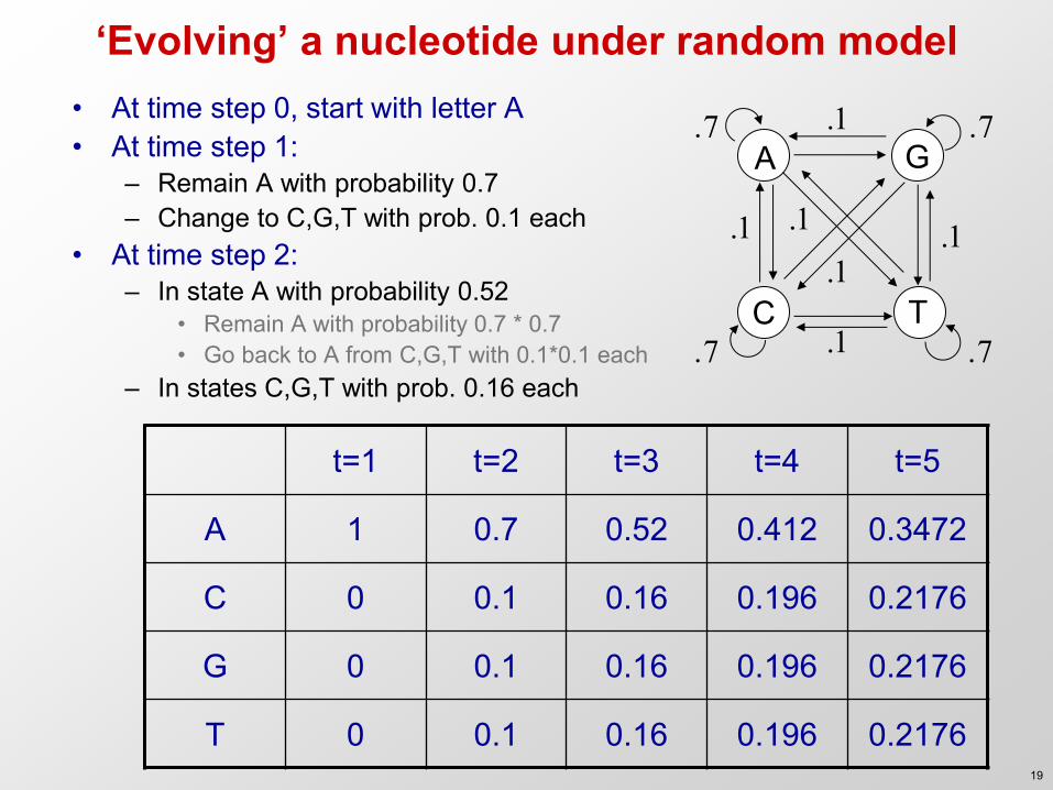
‘Evolving’ a nucleotide under random model
A G
C T
.1
.1 .1
.1
.1
.1
.7 .7
.7 .7
• At time step 0, start with letter A • At time step 1:
– Remain A with probability 0.7 – Change to C,G,T with prob. 0.1 each
• At time step 2: – In state A with probability 0.52
• Remain A with probability 0.7 * 0.7 • Go back to A from C,G,T with 0.1*0.1 each
– In states C,G,T with prob. 0.16 each
t=1 t=2 t=3 t=4 t=5
A 1 0.7 0.52 0.412 0.3472
C 0 0.1 0.16 0.196 0.2176
G 0 0.1 0.16 0.196 0.2176
T 0 0.1 0.16 0.196 0.2176 19
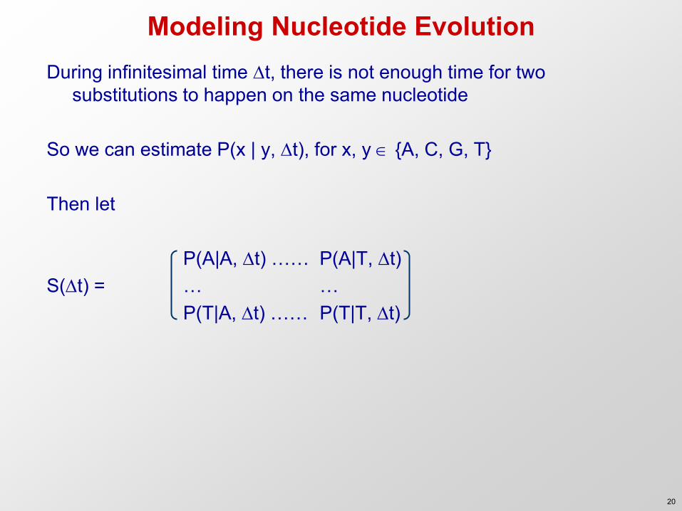
Modeling Nucleotide Evolution During infinitesimal time t, there is not enough time for two
substitutions to happen on the same nucleotide So we can estimate P(x | y, t), for x, y {A, C, G, T} Then let P(A|A, t) …… P(A|T, t) S(t) = … … P(T|A, t) …… P(T|T, t)
20
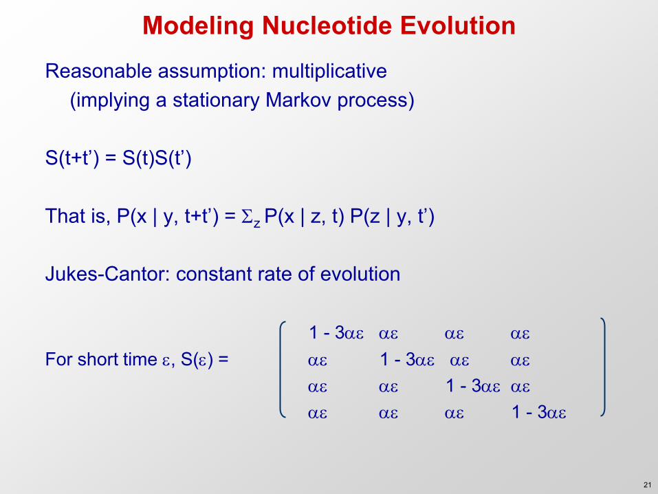
Modeling Nucleotide Evolution Reasonable assumption: multiplicative (implying a stationary Markov process) S(t+t’) = S(t)S(t’) That is, P(x | y, t+t’) = z P(x | z, t) P(z | y, t’) Jukes-Cantor: constant rate of evolution 1 - 3 For short time , S() = 1 - 3 1 - 3 1 - 3
21
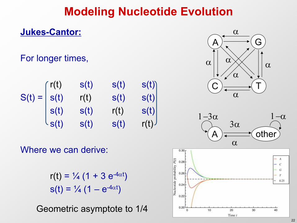
Modeling Nucleotide Evolution Jukes-Cantor: For longer times, r(t) s(t) s(t) s(t) S(t) = s(t) r(t) s(t) s(t) s(t) s(t) r(t) s(t) s(t) s(t) s(t) r(t) Where we can derive: r(t) = ¼ (1 + 3 e-4t) s(t) = ¼ (1 – e-4t)
A G
C T
A other 3
1-3
1-
Geometric asymptote to 1/4 22
Modeling Nucleotide Evolution
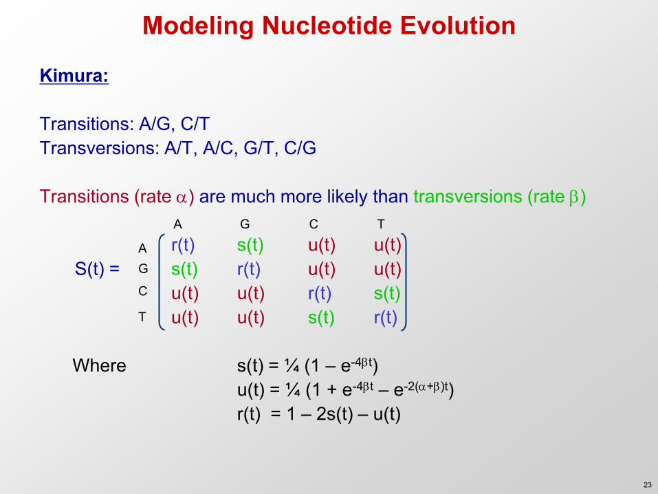
Kimura: Transitions: A/G, C/T Transversions: A/T, A/C, G/T, C/G Transitions (rate ) are much more likely than transversions (rate ) r(t) s(t) u(t) u(t) S(t) = s(t) r(t) u(t) u(t) u(t) u(t) r(t) s(t) u(t) u(t) s(t) r(t)
Where s(t) = ¼ (1 – e-4t) u(t) = ¼ (1 + e-4t – e-2(+)t) r(t) = 1 – 2s(t) – u(t)
A G C T
A G
C
T
23
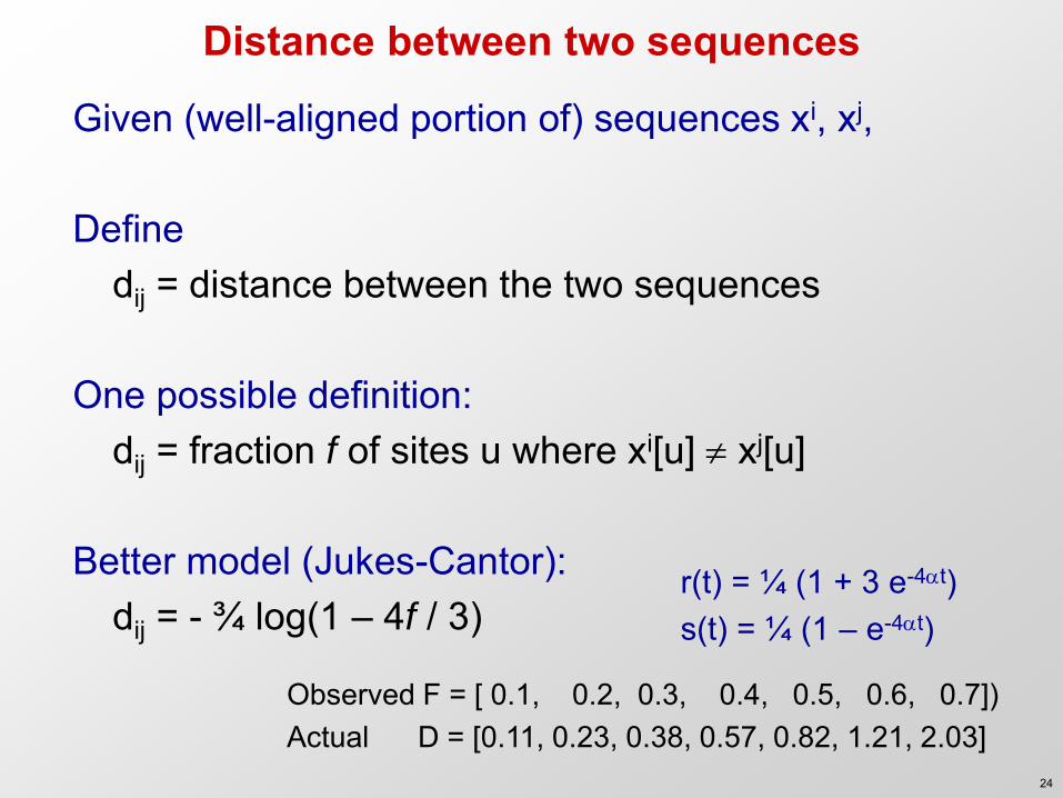
Distance between two sequences
Given (well-aligned portion of) sequences xi, xj, Define dij = distance between the two sequences One possible definition: dij = fraction f of sites u where xi[u] xj[u] Better model (Jukes-Cantor): dij = - ¾ log(1 – 4f / 3)
r(t) = ¼ (1 + 3 e-4t) s(t) = ¼ (1 – e-4t)
Observed F = [ 0.1, 0.2, 0.3, 0.4, 0.5, 0.6, 0.7]) Actual D = [0.11, 0.23, 0.38, 0.57, 0.82, 1.21, 2.03]
24
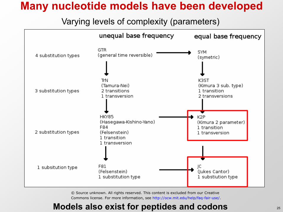
Many nucleotide models have been developed Varying levels of complexity (parameters)
Models also exist for peptides and codons
© Source unknown. All rights reserved. This content is excluded from our Creative
Commons license. For more information, see http://ocw.mit.edu/help/faq-fair-use/.
25
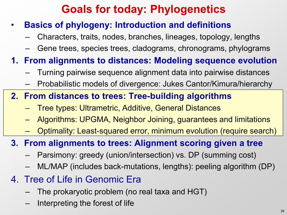
Goals for today: Phylogenetics • Basics of phylogeny: Introduction and definitions
– Characters, traits, nodes, branches, lineages, topology, lengths – Gene trees, species trees, cladograms, chronograms, phylograms
1. From alignments to distances: Modeling sequence evolution – Turning pairwise sequence alignment data into pairwise distances – Probabilistic models of divergence: Jukes Cantor/Kimura/hierarchy
2. From distances to trees: Tree-building algorithms – Tree types: Ultrametric, Additive, General Distances – Algorithms: UPGMA, Neighbor Joining, guarantees and limitations – Optimality: Least-squared error, minimum evolution (require search)
3. From alignments to trees: Alignment scoring given a tree – Parsimony: greedy (union/intersection) vs. DP (summing cost) – ML/MAP (includes back-mutations, lengths): peeling algorithm (DP)
4. Tree of Life in Genomic Era – The prokaryotic problem (no real taxa and HGT) – Interpreting the forest of life
26
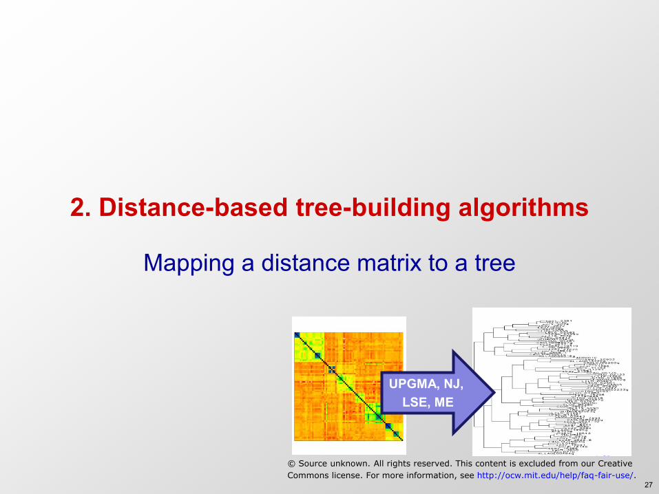
2. Distance-based tree-building algorithms
Mapping a distance matrix to a tree
UPGMA, NJ, LSE, ME
27
© Source unknown. All rights reserved. This content is excluded from our Creative
Commons license. For more information, see http://ocw.mit.edu/help/faq-fair-use/.
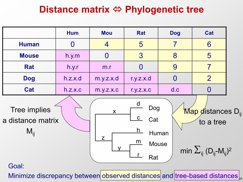
Distance matrix Phylogenetic tree
Hum Mou Rat Dog Cat
Human 0 4 5 7 6 Mouse h.y.m 0 3 8 5
Rat h.y.r m.r 0 9 7 Dog h.z.x.d m.y.z.x.d r.y.z.x.d 0 2 Cat h.z.x.c m.y.z.x.c r.y.z.x.c d.c 0
Human
Dog
Cat
Mouse
Rat
d
c x
h z m
y r
Goal: Minimize discrepancy between observed distances and tree-based distances
Map distances Dij
to a tree Tree implies
a distance matrix Mij
min ij (Dij-Mij)2
28
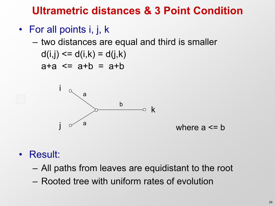
Ultrametric distances & 3 Point Condition • For all points i, j, k
– two distances are equal and third is smaller d(i,j) <= d(i,k) = d(j,k) a+a <= a+b = a+b
a
a
b
i
j
k
where a <= b
• Result: – All paths from leaves are equidistant to the root – Rooted tree with uniform rates of evolution
29
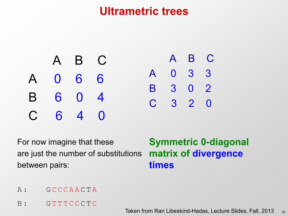
Ultrametric trees
A B C A 0 3 3 B 3 0 2 C 3 2 0
Symmetric 0-diagonal matrix of divergence times
A B C A 0 6 6 B 6 0 4 C 6 4 0
For now imagine that these are just the number of substitutions between pairs: A: GCCCAACTA
B: GTTTCCCTC Taken from Ran Libeskind-Hadas, Lecture Slides, Fall, 2013 30
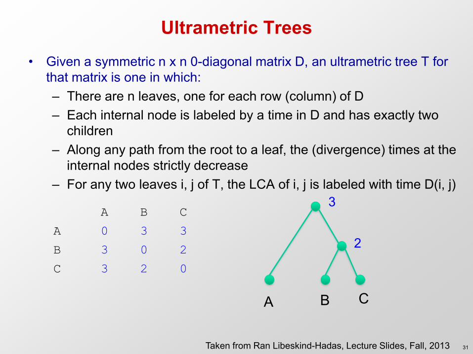
Ultrametric Trees
• Given a symmetric n x n 0-diagonal matrix D, an ultrametric tree T for that matrix is one in which: – There are n leaves, one for each row (column) of D – Each internal node is labeled by a time in D and has exactly two
children – Along any path from the root to a leaf, the (divergence) times at the
internal nodes strictly decrease – For any two leaves i, j of T, the LCA of i, j is labeled with time D(i, j)
A B C
A 0 3 3
B 3 0 2
C 3 2 0
3
2
A B C
Taken from Ran Libeskind-Hadas, Lecture Slides, Fall, 2013 31
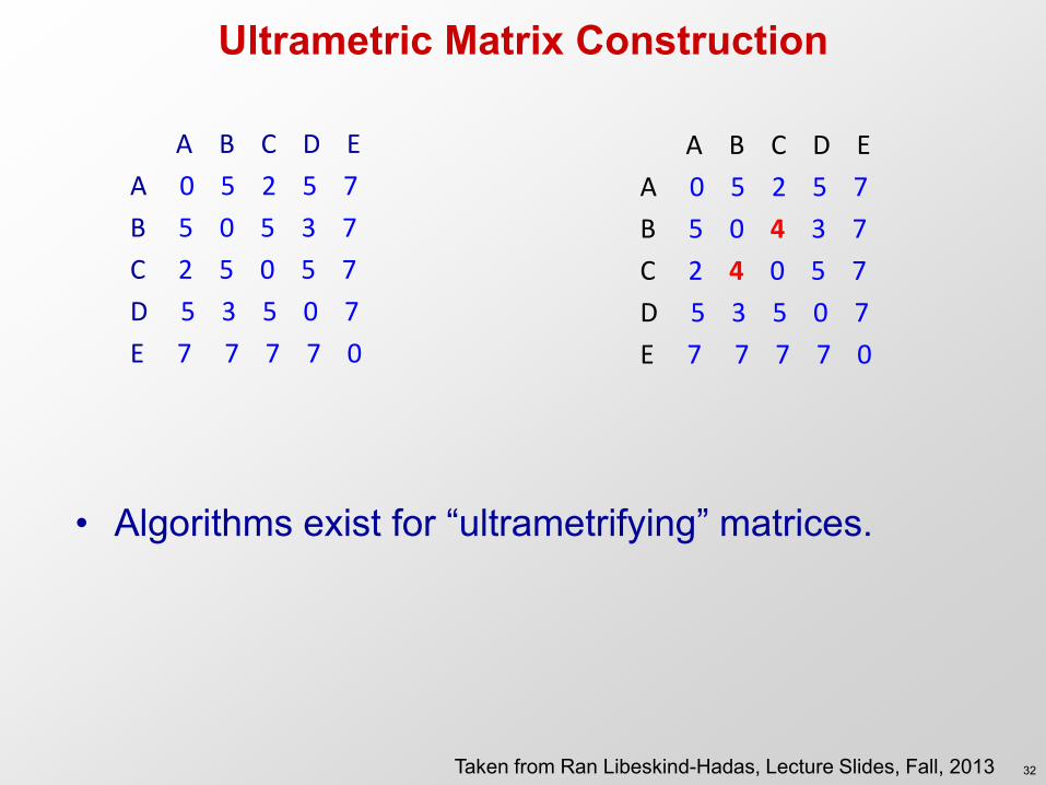
Ultrametric Matrix Construction
A B C D E
A 0 5 2 5 7
B 5 0 5 3 7
C 2 5 0 5 7
D 5 3 5 0 7
E 7 7 7 7 0
A B C D E
A 0 5 2 5 7
B 5 0 4 3 7
C 2 4 0 5 7
D 5 3 5 0 7
E 7 7 7 7 0
• Algorithms exist for “ultrametrifying” matrices.
Taken from Ran Libeskind-Hadas, Lecture Slides, Fall, 2013 32
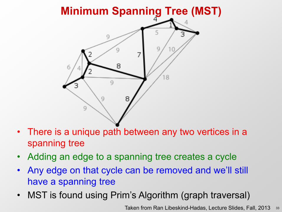
Minimum Spanning Tree (MST)
• There is a unique path between any two vertices in a spanning tree
• Adding an edge to a spanning tree creates a cycle • Any edge on that cycle can be removed and we’ll still
have a spanning tree • MST is found using Prim’s Algorithm (graph traversal)
Taken from Ran Libeskind-Hadas, Lecture Slides, Fall, 2013 33
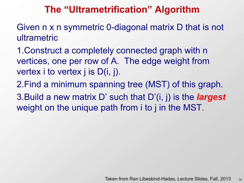
The “Ultrametrification” Algorithm
Given n x n symmetric 0-diagonal matrix D that is not ultrametric 1.Construct a completely connected graph with n vertices, one per row of A. The edge weight from vertex i to vertex j is D(i, j). 2.Find a minimum spanning tree (MST) of this graph. 3.Build a new matrix D’ such that D’(i, j) is the largest weight on the unique path from i to j in the MST.
Taken from Ran Libeskind-Hadas, Lecture Slides, Fall, 2013 34
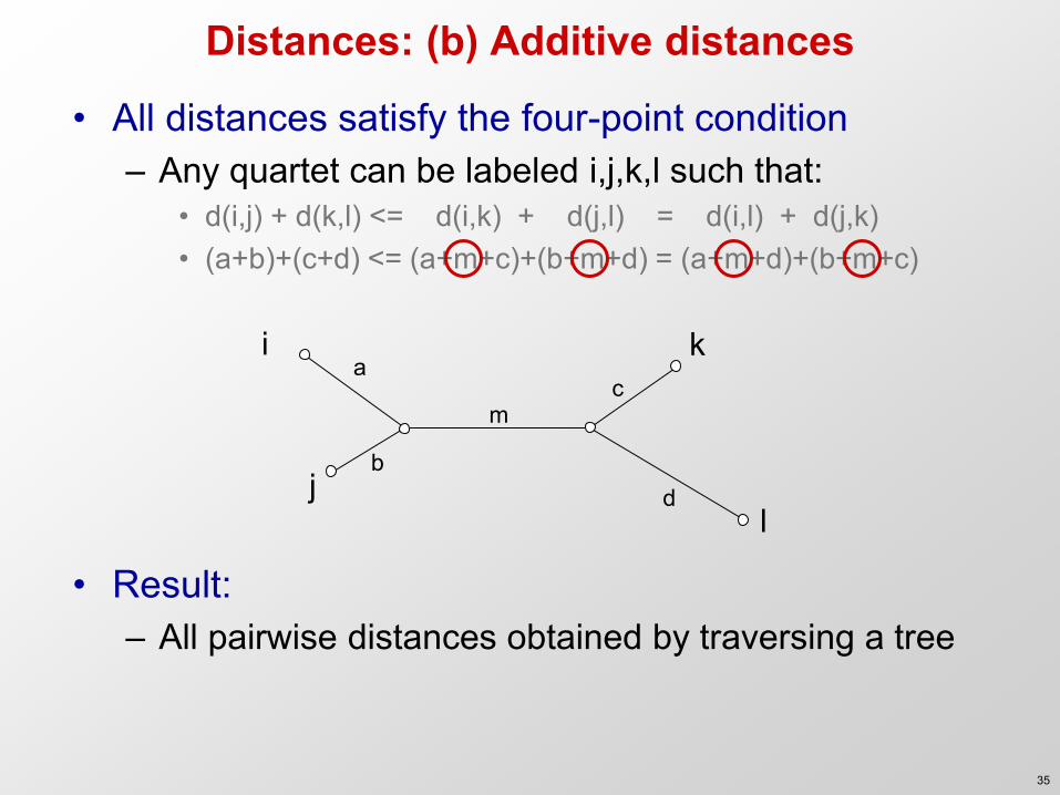
Distances: (b) Additive distances
• All distances satisfy the four-point condition – Any quartet can be labeled i,j,k,l such that:
• d(i,j) + d(k,l) <= d(i,k) + d(j,l) = d(i,l) + d(j,k) • (a+b)+(c+d) <= (a+m+c)+(b+m+d) = (a+m+d)+(b+m+c)
• Result: – All pairwise distances obtained by traversing a tree
a
b
m
i
j
k
l
c
d
35
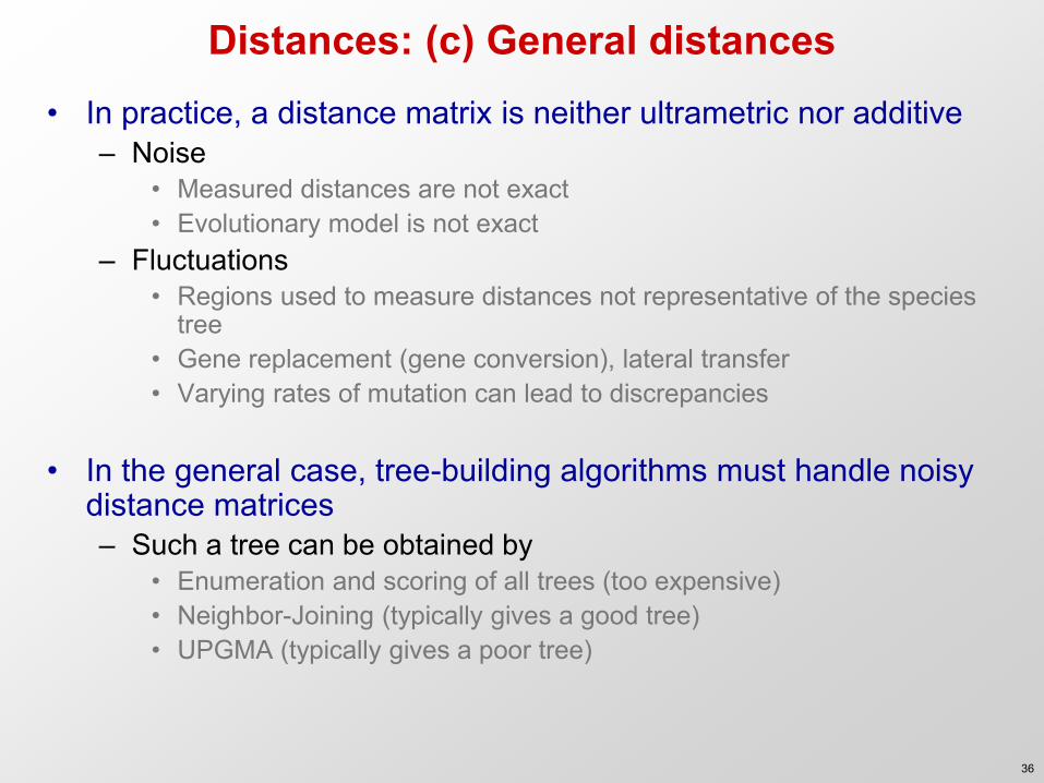
Distances: (c) General distances • In practice, a distance matrix is neither ultrametric nor additive
– Noise • Measured distances are not exact • Evolutionary model is not exact
– Fluctuations • Regions used to measure distances not representative of the species
tree • Gene replacement (gene conversion), lateral transfer • Varying rates of mutation can lead to discrepancies
• In the general case, tree-building algorithms must handle noisy
distance matrices – Such a tree can be obtained by
• Enumeration and scoring of all trees (too expensive) • Neighbor-Joining (typically gives a good tree) • UPGMA (typically gives a poor tree)
36
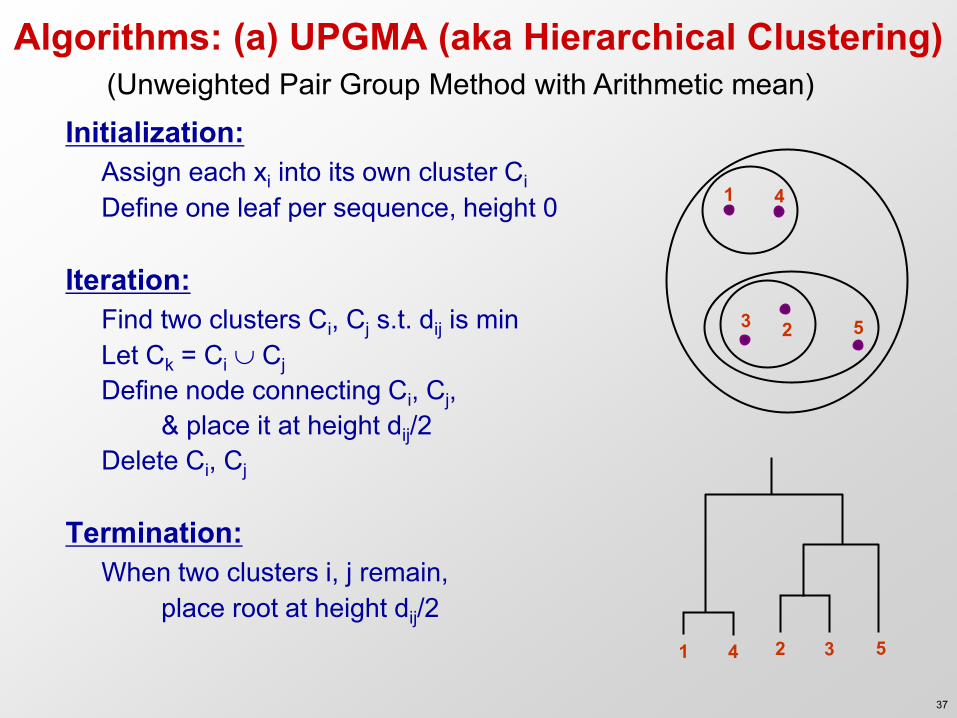
Algorithms: (a) UPGMA (aka Hierarchical Clustering)
Initialization: Assign each xi into its own cluster Ci Define one leaf per sequence, height 0 Iteration: Find two clusters Ci, Cj s.t. dij is min Let Ck = Ci Cj Define node connecting Ci, Cj, & place it at height dij/2
Delete Ci, Cj Termination: When two clusters i, j remain, place root at height dij/2
1 4
3 2 5
1 4 2 3 5
(Unweighted Pair Group Method with Arithmetic mean)
37
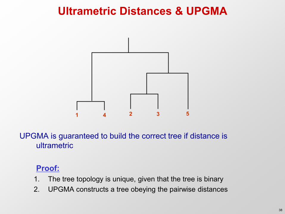
Ultrametric Distances & UPGMA
UPGMA is guaranteed to build the correct tree if distance is ultrametric
Proof:
1. The tree topology is unique, given that the tree is binary 2. UPGMA constructs a tree obeying the pairwise distances
1 4 2 3 5
38
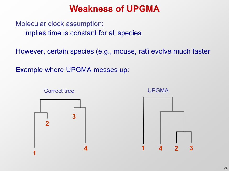
Weakness of UPGMA Molecular clock assumption: implies time is constant for all species However, certain species (e.g., mouse, rat) evolve much faster Example where UPGMA messes up:
2 3
4 1
1 4 3 2
Correct tree UPGMA
39
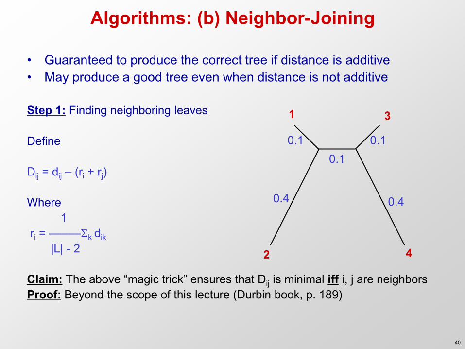
Algorithms: (b) Neighbor-Joining
• Guaranteed to produce the correct tree if distance is additive • May produce a good tree even when distance is not additive
Step 1: Finding neighboring leaves Define Dij = dij – (ri + rj) Where 1 ri = –––––k dik |L| - 2 Claim: The above “magic trick” ensures that Dij is minimal iff i, j are neighbors Proof: Beyond the scope of this lecture (Durbin book, p. 189)
1
2 4
3
0.1 0.1 0.1
0.4 0.4
40
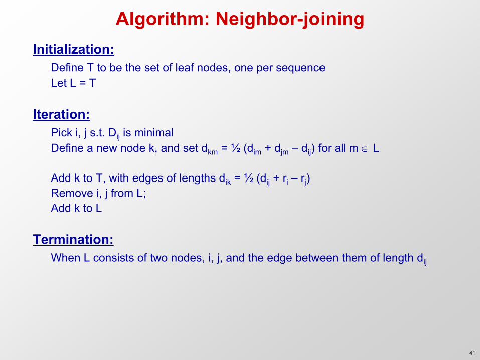
Algorithm: Neighbor-joining Initialization: Define T to be the set of leaf nodes, one per sequence Let L = T Iteration: Pick i, j s.t. Dij is minimal Define a new node k, and set dkm = ½ (dim + djm – dij) for all m L Add k to T, with edges of lengths dik = ½ (dij + ri – rj) Remove i, j from L; Add k to L Termination: When L consists of two nodes, i, j, and the edge between them of length dij
41
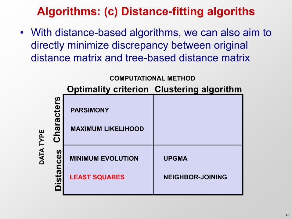
COMPUTATIONAL METHOD
Clustering algorithm Optimality criterion
DAT
A TY
PE
Cha
ract
ers
Dis
tanc
es
PARSIMONY MAXIMUM LIKELIHOOD
UPGMA NEIGHBOR-JOINING
MINIMUM EVOLUTION LEAST SQUARES
Algorithms: (c) Distance-fitting algoriths
• With distance-based algorithms, we can also aim to directly minimize discrepancy between original distance matrix and tree-based distance matrix
42

Distance matrix Phylogenetic tree
Hum Mou Rat Dog Cat
Human 0 4 5 7 6 Mouse h.y.m 0 3 8 5
Rat h.y.r m.r 0 9 7 Dog h.z.x.d m.y.z.x.d r.y.z.x.d 0 2 Cat h.z.x.c m.y.z.x.c r.y.z.x.c d.c 0
Human
Dog
Cat
Mouse
Rat
d
c x
h z m
y r
Goal: Minimize discrepancy between observed distances and tree-based distances
Map distances Dij
to a tree Tree implies
a distance matrix Mij
min ij (Dij-Mij)2
43
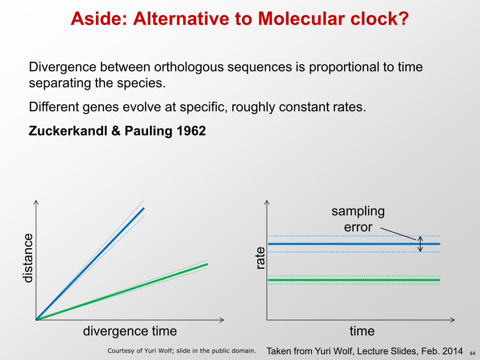
Aside: Alternative to Molecular clock?
Divergence between orthologous sequences is proportional to time separating the species.
Different genes evolve at specific, roughly constant rates.
Zuckerkandl & Pauling 1962
divergence time
dist
ance
time
rate
sampling error
Taken from Yuri Wolf, Lecture Slides, Feb. 2014 Courtesy of Yuri Wolf; slide in the public domain. 44
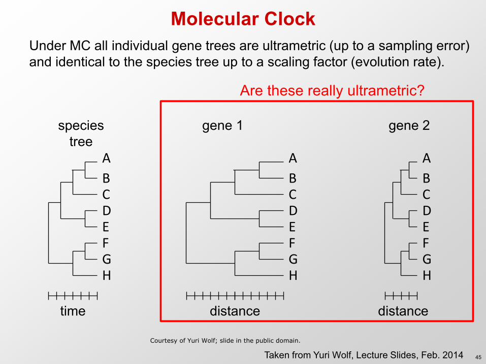
Molecular Clock Under MC all individual gene trees are ultrametric (up to a sampling error) and identical to the species tree up to a scaling factor (evolution rate).
A
B C D E F G H
time
A
B C D E F G H
distance
A
B C D E F G H
distance
species tree
gene 1 gene 2
Taken from Yuri Wolf, Lecture Slides, Feb. 2014
Are these really ultrametric?
Courtesy of Yuri Wolf; slide in the public domain.
45
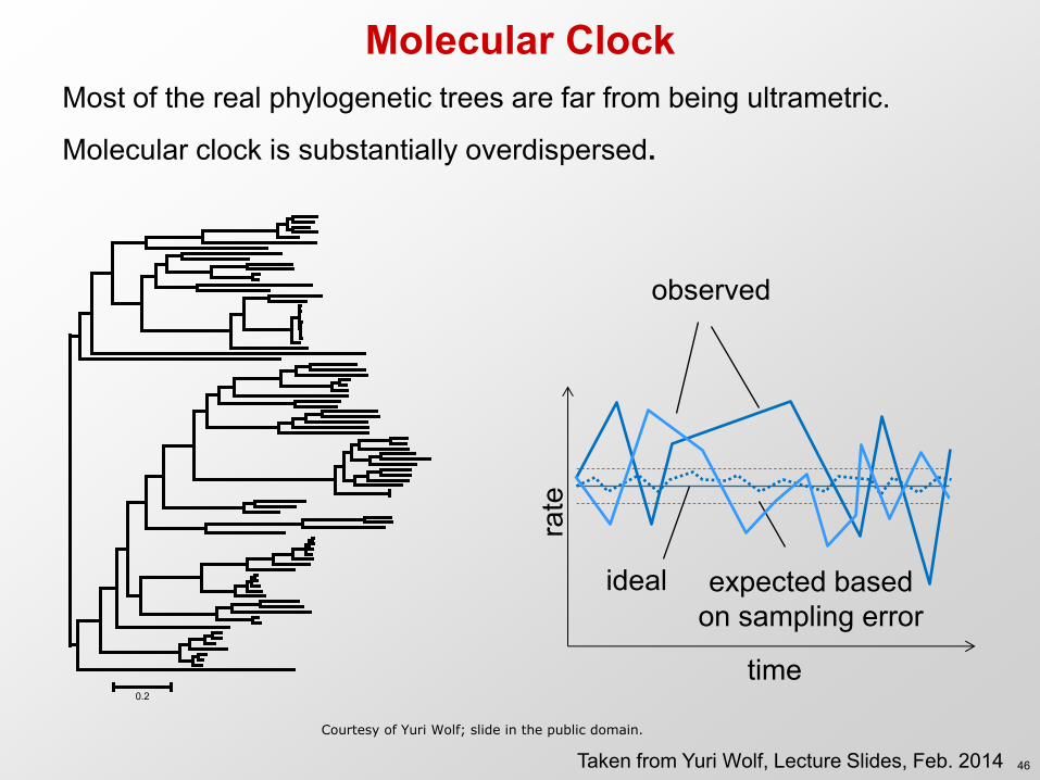
Molecular Clock Most of the real phylogenetic trees are far from being ultrametric.
Molecular clock is substantially overdispersed.
time
rate
0.2
ideal expected based on sampling error
observed
Taken from Yuri Wolf, Lecture Slides, Feb. 2014 Courtesy of Yuri Wolf; slide in the public domain.
46
Relaxed Molecular Clock
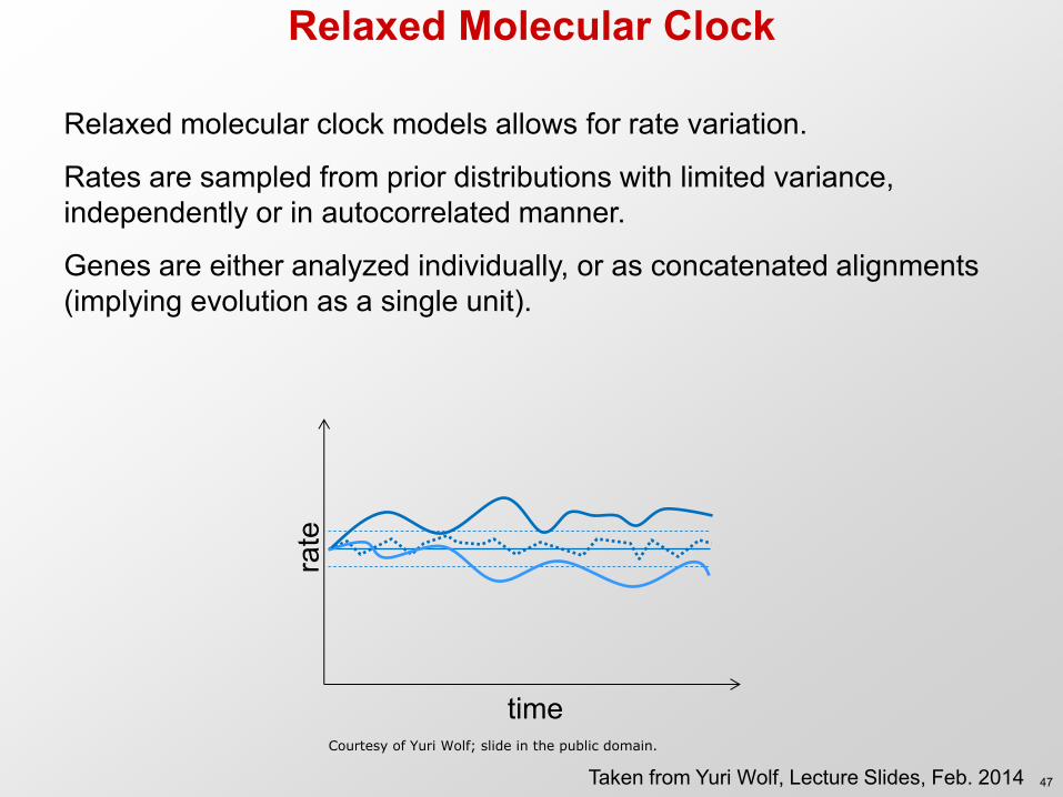
Relaxed molecular clock models allows for rate variation.
Rates are sampled from prior distributions with limited variance, independently or in autocorrelated manner.
Genes are either analyzed individually, or as concatenated alignments (implying evolution as a single unit).
time
rate
Taken from Yuri Wolf, Lecture Slides, Feb. 2014 Courtesy of Yuri Wolf; slide in the public domain.
47
Universal Pacemaker
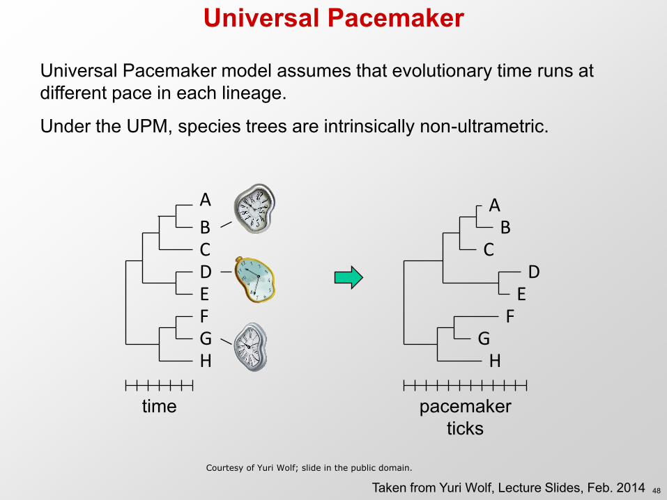
Universal Pacemaker model assumes that evolutionary time runs at different pace in each lineage.
Under the UPM, species trees are intrinsically non-ultrametric.
A
B C D E F G H
A B
C D
E F
G H
time pacemaker ticks
Taken from Yuri Wolf, Lecture Slides, Feb. 2014 Courtesy of Yuri Wolf; slide in the public domain.
48
Pacemaker vs Clock
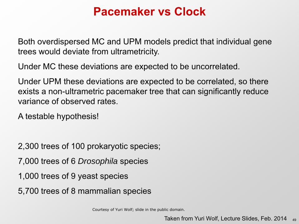
Both overdispersed MC and UPM models predict that individual gene trees would deviate from ultrametricity.
Under MC these deviations are expected to be uncorrelated.
Under UPM these deviations are expected to be correlated, so there exists a non-ultrametric pacemaker tree that can significantly reduce variance of observed rates.
A testable hypothesis!
2,300 trees of 100 prokaryotic species;
7,000 trees of 6 Drosophila species
1,000 trees of 9 yeast species
5,700 trees of 8 mammalian species
Taken from Yuri Wolf, Lecture Slides, Feb. 2014 Courtesy of Yuri Wolf; slide in the public domain.
49
Pacemaker vs Clock
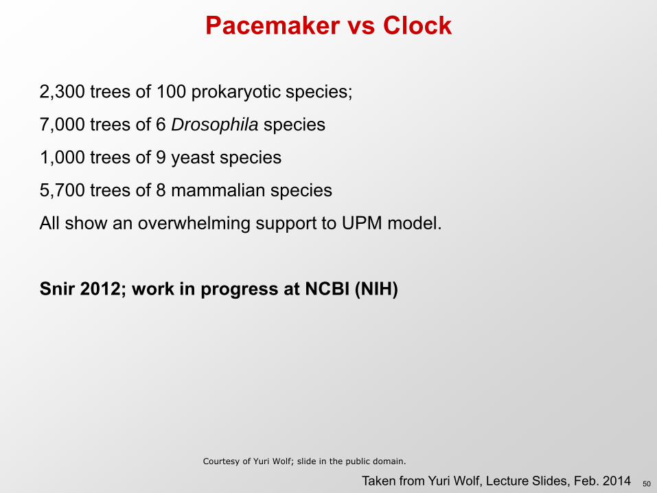
2,300 trees of 100 prokaryotic species;
7,000 trees of 6 Drosophila species
1,000 trees of 9 yeast species
5,700 trees of 8 mammalian species
All show an overwhelming support to UPM model.
Snir 2012; work in progress at NCBI (NIH)
Taken from Yuri Wolf, Lecture Slides, Feb. 2014 Courtesy of Yuri Wolf; slide in the public domain.
50
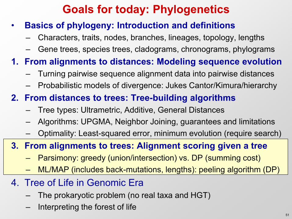
Goals for today: Phylogenetics • Basics of phylogeny: Introduction and definitions
– Characters, traits, nodes, branches, lineages, topology, lengths – Gene trees, species trees, cladograms, chronograms, phylograms
1. From alignments to distances: Modeling sequence evolution – Turning pairwise sequence alignment data into pairwise distances – Probabilistic models of divergence: Jukes Cantor/Kimura/hierarchy
2. From distances to trees: Tree-building algorithms – Tree types: Ultrametric, Additive, General Distances – Algorithms: UPGMA, Neighbor Joining, guarantees and limitations – Optimality: Least-squared error, minimum evolution (require search)
3. From alignments to trees: Alignment scoring given a tree – Parsimony: greedy (union/intersection) vs. DP (summing cost) – ML/MAP (includes back-mutations, lengths): peeling algorithm (DP)
4. Tree of Life in Genomic Era – The prokaryotic problem (no real taxa and HGT) – Interpreting the forest of life
51
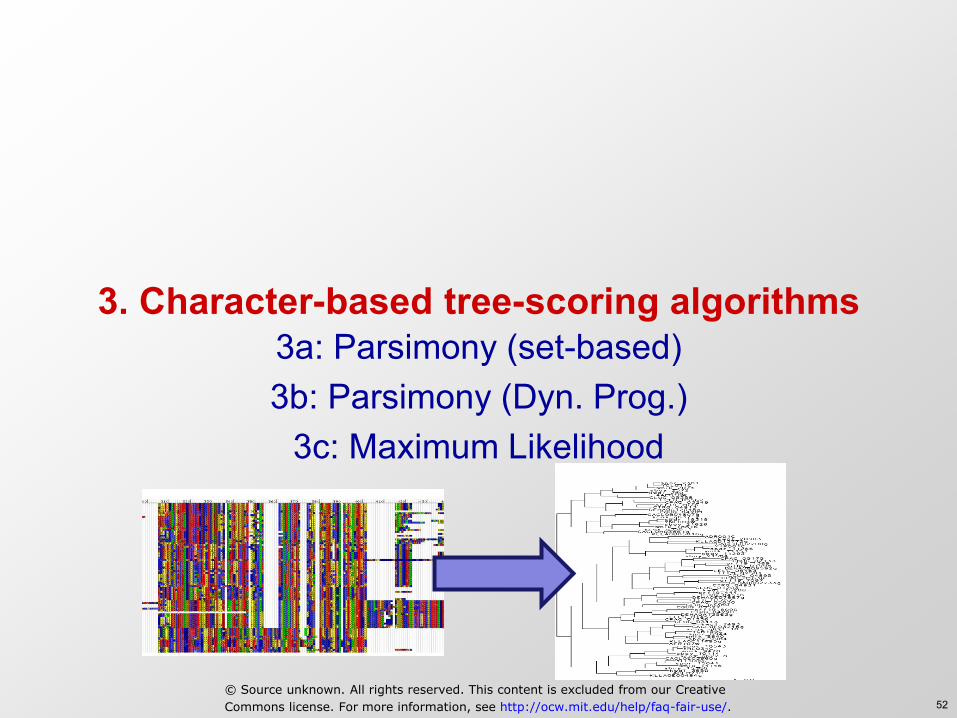
3. Character-based tree-scoring algorithms 3a: Parsimony (set-based) 3b: Parsimony (Dyn. Prog.)
3c: Maximum Likelihood
52© Source unknown. All rights reserved. This content is excluded from our Creative
Commons license. For more information, see http://ocw.mit.edu/help/faq-fair-use/.
Basic algorithms of phylogenetic methods
Distance based
Character based
From alignments To phylogenies
From Sequences To Distances
Tree building algorithms
Pair-wise distance matrix Sequence alignment
Sequence alignment Output tree
Output tree
Couple to tree proposal and scoring
1 2
3
4 53
© Source unknown. All rights reserved. This content is excluded from our Creative
Commons license. For more information, see http://ocw.mit.edu/help/faq-fair-use/.
Character-based phylogenetic inference
• Really about tree scoring techniques, not tree finding techniques – Couple them with tree proposal and update and you
have an algorithm (part 4 of the lecture) • Two approaches exist, all use same architecture:
– Minimize events: Parsimony (union/intersection) – Probabilistic: Max Likelihood / MAP
54
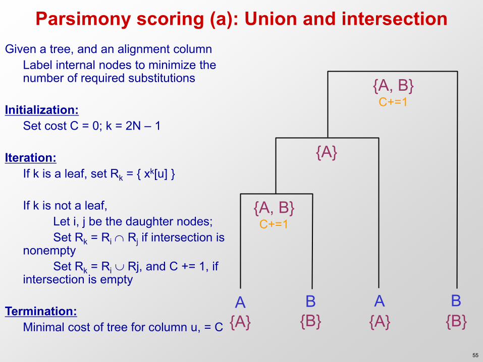
Parsimony scoring (a): Union and intersection
A B A B
{A, B} C+=1
{A, B} C+=1
{A}
{A} {B} {A} {B}
Given a tree, and an alignment column Label internal nodes to minimize the
number of required substitutions Initialization: Set cost C = 0; k = 2N – 1 Iteration: If k is a leaf, set Rk = { xk[u] } If k is not a leaf, Let i, j be the daughter nodes; Set Rk = Ri Rj if intersection is
nonempty Set Rk = Ri Rj, and C += 1, if
intersection is empty Termination: Minimal cost of tree for column u, = C
55
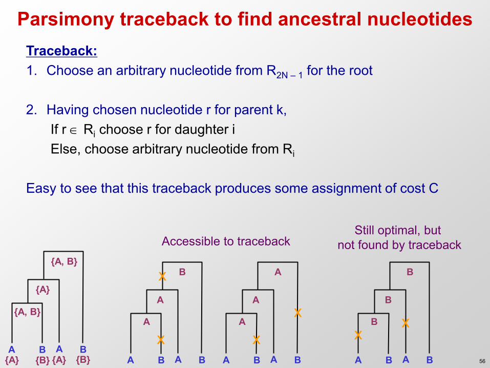
Parsimony traceback to find ancestral nucleotides
A B A B
{A, B}
{A, B}
{A}
{A} {B} {A} {B} A B A B
A
A
A x
x A B A B
A
B
A
x
x A B A B
B
B
B
x x
Accessible to traceback Still optimal, but
not found by traceback
Traceback: 1. Choose an arbitrary nucleotide from R2N – 1 for the root
2. Having chosen nucleotide r for parent k,
If r Ri choose r for daughter i Else, choose arbitrary nucleotide from Ri
Easy to see that this traceback produces some assignment of cost C
56
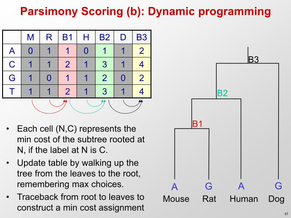
Parsimony Scoring (b): Dynamic programming
M R B1 H B2 D B3 A 0 1 1 0 1 1 2 C 1 1 2 1 3 1 4 G 1 0 1 1 2 0 2 T 1 1 2 1 3 1 4
• Each cell (N,C) represents the min cost of the subtree rooted at N, if the label at N is C.
• Update table by walking up the tree from the leaves to the root, remembering max choices.
• Traceback from root to leaves to construct a min cost assignment
A G A G Mouse Rat Human Dog
B1
B2
B3
57
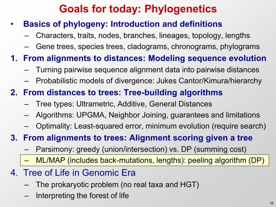
Goals for today: Phylogenetics • Basics of phylogeny: Introduction and definitions
– Characters, traits, nodes, branches, lineages, topology, lengths – Gene trees, species trees, cladograms, chronograms, phylograms
1. From alignments to distances: Modeling sequence evolution – Turning pairwise sequence alignment data into pairwise distances – Probabilistic models of divergence: Jukes Cantor/Kimura/hierarchy
2. From distances to trees: Tree-building algorithms – Tree types: Ultrametric, Additive, General Distances – Algorithms: UPGMA, Neighbor Joining, guarantees and limitations – Optimality: Least-squared error, minimum evolution (require search)
3. From alignments to trees: Alignment scoring given a tree – Parsimony: greedy (union/intersection) vs. DP (summing cost) – ML/MAP (includes back-mutations, lengths): peeling algorithm (DP)
4. Tree of Life in Genomic Era – The prokaryotic problem (no real taxa and HGT) – Interpreting the forest of life
58
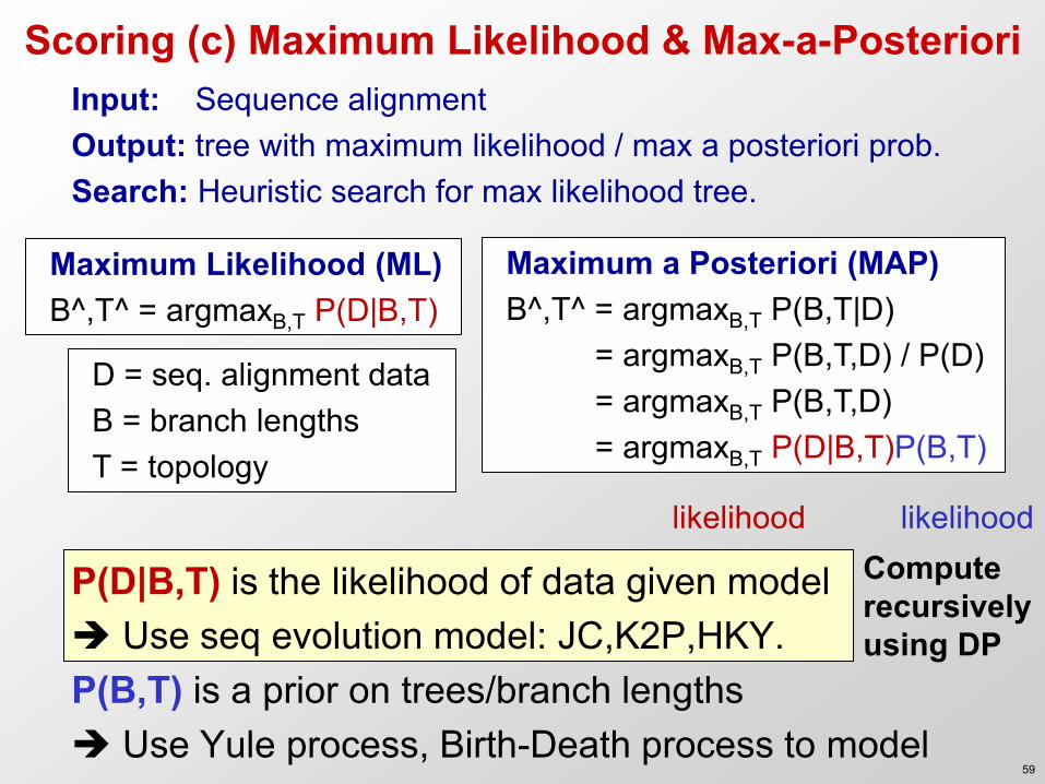
Compute recursively using DP
Scoring (c) Maximum Likelihood & Max-a-Posteriori Input: Sequence alignment Output: tree with maximum likelihood / max a posteriori prob. Search: Heuristic search for max likelihood tree.
P(D|B,T) is the likelihood of data given model Use seq evolution model: JC,K2P,HKY. P(B,T) is a prior on trees/branch lengths Use Yule process, Birth-Death process to model
Maximum Likelihood (ML) B^,T^ = argmaxB,T P(D|B,T)
Maximum a Posteriori (MAP) B^,T^ = argmaxB,T P(B,T|D) = argmaxB,T P(B,T,D) / P(D) = argmaxB,T P(B,T,D) = argmaxB,T P(D|B,T)P(B,T)
D = seq. alignment data B = branch lengths T = topology
likelihood likelihood
59
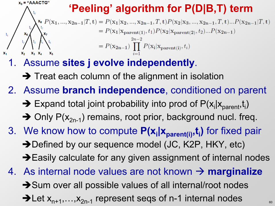
‘Peeling’ algorithm for P(D|B,T) term
1. Assume sites j evolve independently. Treat each column of the alignment in isolation
2. Assume branch independence, conditioned on parent Expand total joint probability into prod of P(xi|xparent,ti) Only P(x2n-1) remains, root prior, background nucl. freq.
3. We know how to compute P(xi|xparent(i),ti) for fixed pair Defined by our sequence model (JC, K2P, HKY, etc) Easily calculate for any given assignment of internal nodes
4. As internal node values are not known marginalize Sum over all possible values of all internal/root nodes Let xn+1,…,x2n-1 represent seqs of n-1 internal nodes 60
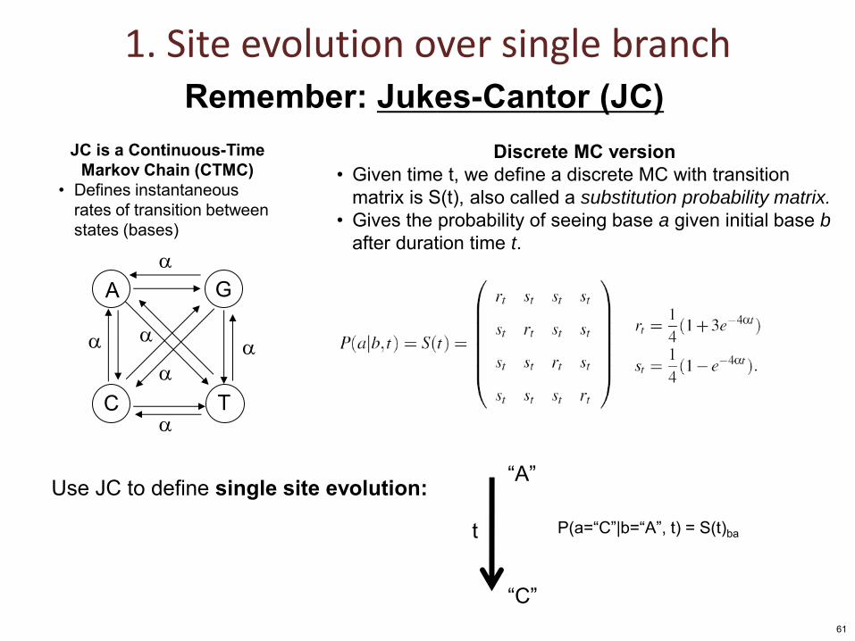
1. Site evolution over single branch
A G
C T
JC is a Continuous-Time Markov Chain (CTMC)
• Defines instantaneous rates of transition between states (bases)
Use JC to define single site evolution: “A”
“C”
t P(a=“C”|b=“A”, t) = S(t)ba
Remember: Jukes-Cantor (JC) Discrete MC version
• Given time t, we define a discrete MC with transition matrix is S(t), also called a substitution probability matrix.
• Gives the probability of seeing base a given initial base b after duration time t.
61
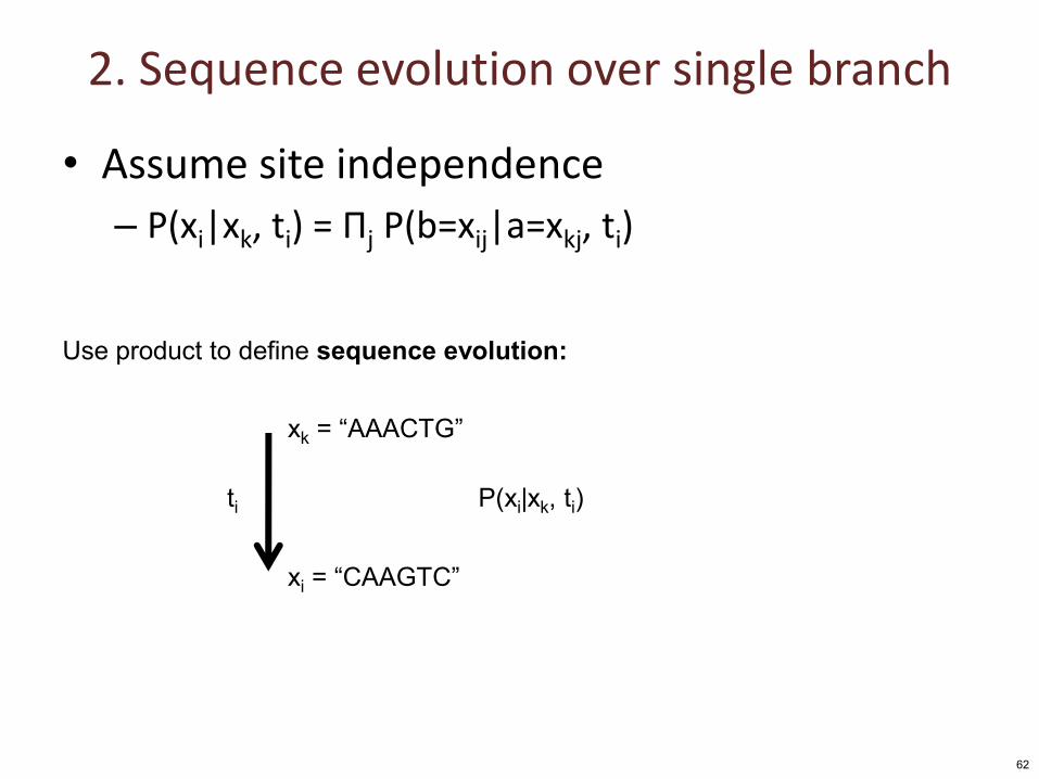
2. Sequence evolution over single branch
• Assume site independence
– P(xi|xk, ti) = Πj P(b=xij|a=xkj, ti)
Use product to define sequence evolution:
xk = “AAACTG”
xi = “CAAGTC”
ti P(xi|xk, ti)
62
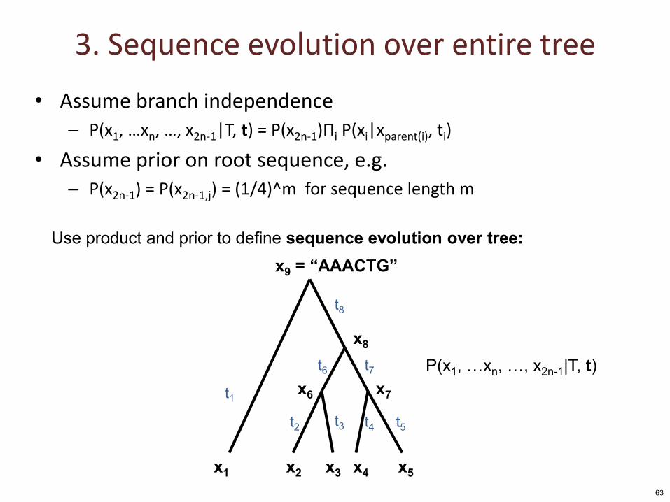
3. Sequence evolution over entire tree
• Assume branch independence – P(x1, …xn, …, x2n-1|T, t) = P(x2n-1)Πi P(xi|xparent(i), ti)
• Assume prior on root sequence, e.g. – P(x2n-1) = P(x2n-1,j) = (1/4)^m for sequence length m
Use product and prior to define sequence evolution over tree: x9 = “AAACTG”
x1 x2 x3 x4 x5
x7 x6
x8
t1
t2 t3
t6 t7
t4 t5
t8
P(x1, …xn, …, x2n-1|T, t)
63
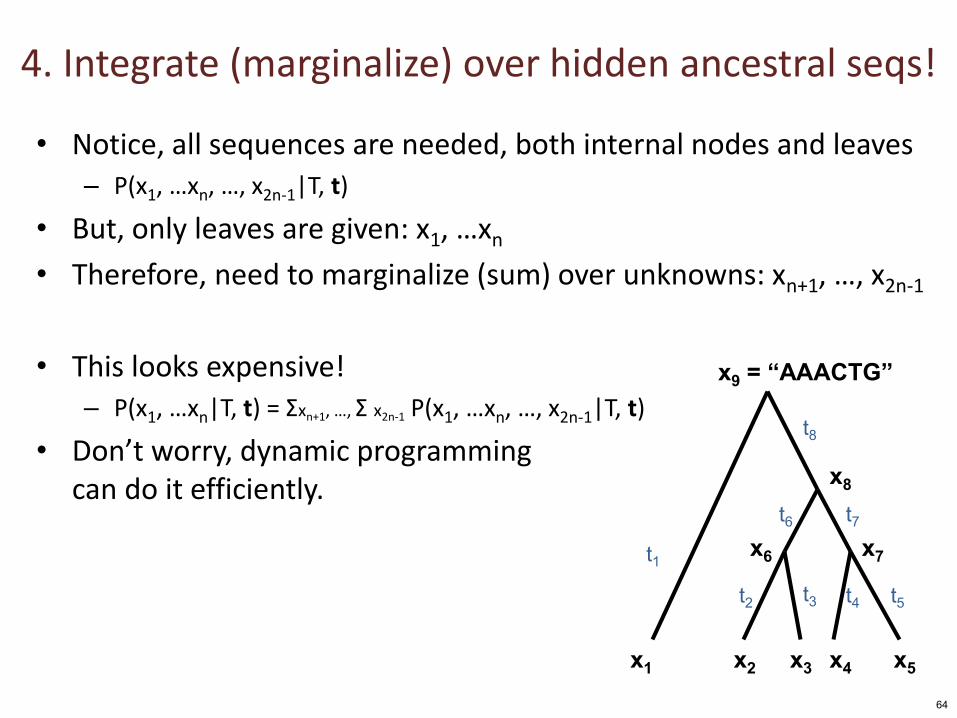
4. Integrate (marginalize) over hidden ancestral seqs!
• Notice, all sequences are needed, both internal nodes and leaves – P(x1, …xn, …, x2n-1|T, t)
• But, only leaves are given: x1, …xn
• Therefore, need to marginalize (sum) over unknowns: xn+1, …, x2n-1
• This looks expensive! – P(x1, …xn|T, t) = Σxn+1, …, Σ x2n-1 P(x1, …xn, …, x2n-1|T, t)
• Don’t worry, dynamic programming can do it efficiently.
x9 = “AAACTG”
x1 x2 x3 x4 x5
x7 x6
x8
t1
t2 t3
t6 t7
t4 t5
t8
64
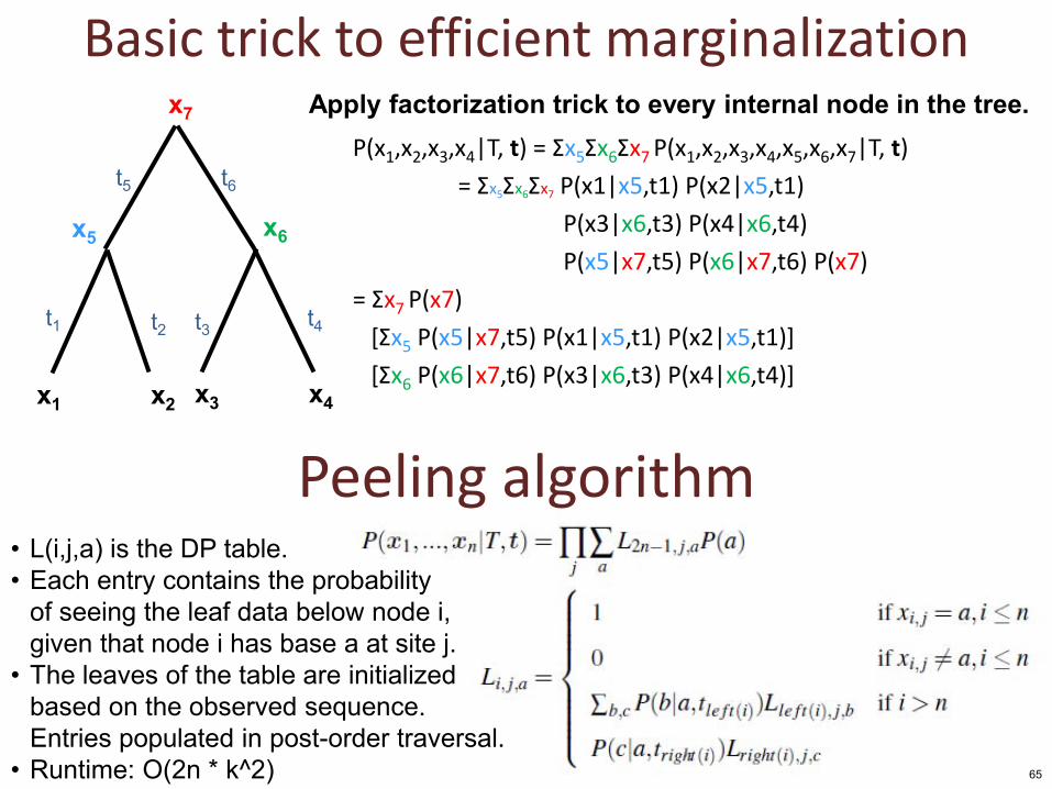
Basic trick to efficient marginalization
P(x1,x2,x3,x4|T, t) = Σx5Σx6Σx7 P(x1,x2,x3,x4,x5,x6,x7|T, t)
= Σx5Σx6Σx7 P(x1|x5,t1) P(x2|x5,t1)
P(x3|x6,t3) P(x4|x6,t4)
P(x5|x7,t5) P(x6|x7,t6) P(x7)
= Σx7 P(x7)
[Σx5 P(x5|x7,t5) P(x1|x5,t1) P(x2|x5,t1)]
[Σx6 P(x6|x7,t6) P(x3|x6,t3) P(x4|x6,t4)]
x5
x1 x2
t1 t2
x6
x3 x4
t3 t4
x7
t5 t6
Apply factorization trick to every internal node in the tree.
• L(i,j,a) is the DP table. • Each entry contains the probability
of seeing the leaf data below node i, given that node i has base a at site j.
• The leaves of the table are initialized based on the observed sequence. Entries populated in post-order traversal.
• Runtime: O(2n * k^2)
Peeling algorithm
65
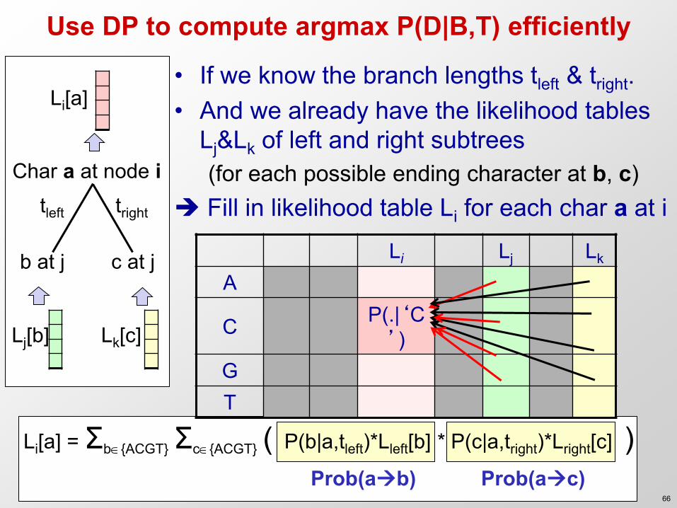
Use DP to compute argmax P(D|B,T) efficiently
• If we know the branch lengths tleft & tright. • And we already have the likelihood tables
Lj&Lk of left and right subtrees (for each possible ending character at b, c)
Fill in likelihood table Li for each char a at i
Lj[b]
Li Lj Lk
A
C P(.|‘C’)
G T
Li[a] = Σb{ACGT} Σc{ACGT} ( P(b|a,tleft)*Lleft[b] * P(c|a,tright)*Lright[c] )
Char a at node i
b at j
Prob(ab)
tleft tright
Lk[c]
Li[a]
Prob(ac)
c at j
66
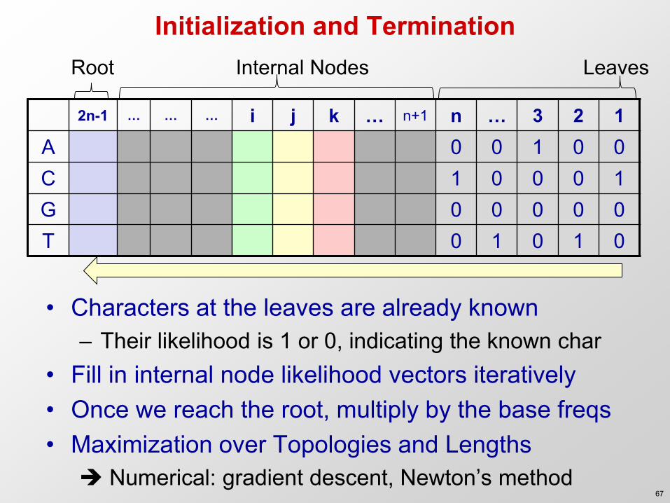
Initialization and Termination
• Characters at the leaves are already known – Their likelihood is 1 or 0, indicating the known char
• Fill in internal node likelihood vectors iteratively • Once we reach the root, multiply by the base freqs • Maximization over Topologies and Lengths Numerical: gradient descent, Newton’s method
2n-1 … … … i j k … n+1 n … 3 2 1 A 0 0 1 0 0 C 1 0 0 0 1 G 0 0 0 0 0 T 0 1 0 1 0
Root Leaves Internal Nodes
67
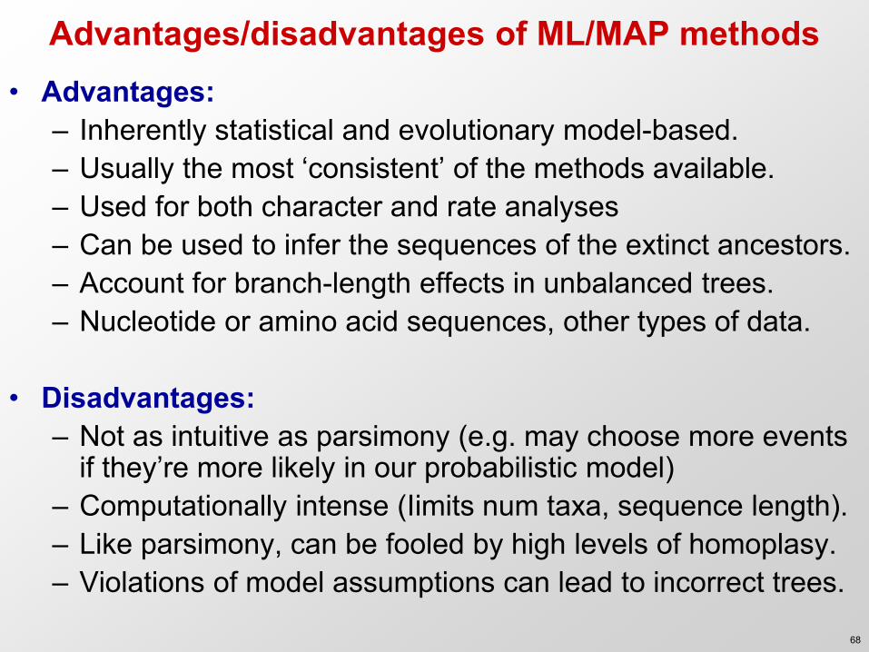
Advantages/disadvantages of ML/MAP methods • Advantages:
– Inherently statistical and evolutionary model-based. – Usually the most ‘consistent’ of the methods available. – Used for both character and rate analyses – Can be used to infer the sequences of the extinct ancestors. – Account for branch-length effects in unbalanced trees. – Nucleotide or amino acid sequences, other types of data.
• Disadvantages:
– Not as intuitive as parsimony (e.g. may choose more events if they’re more likely in our probabilistic model)
– Computationally intense (Iimits num taxa, sequence length). – Like parsimony, can be fooled by high levels of homoplasy. – Violations of model assumptions can lead to incorrect trees.
68
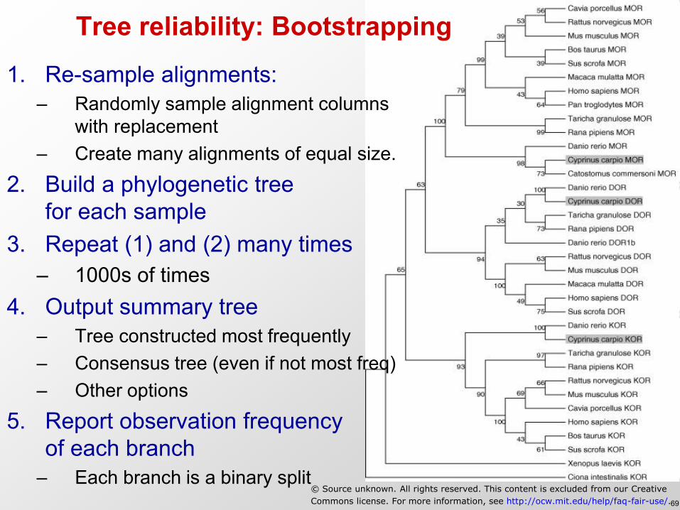
Tree reliability: Bootstrapping
1. Re-sample alignments: – Randomly sample alignment columns
with replacement – Create many alignments of equal size.
2. Build a phylogenetic tree for each sample
3. Repeat (1) and (2) many times – 1000s of times
4. Output summary tree – Tree constructed most frequently – Consensus tree (even if not most freq) – Other options
5. Report observation frequency of each branch
– Each branch is a binary split © Source unknown. All rights reserved. This content is excluded from our Creative
Commons license. For more information, see http://ocw.mit.edu/help/faq-fair-use/.69
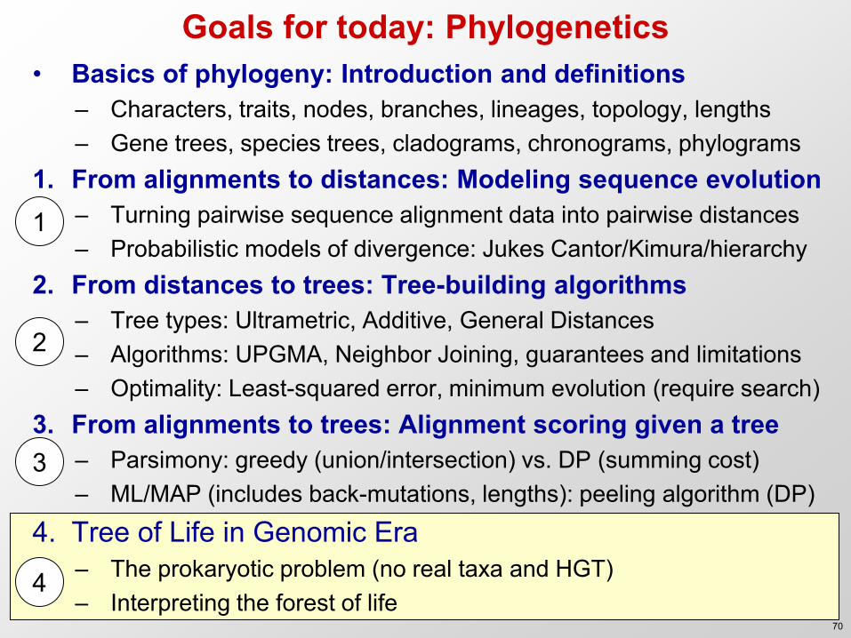
Goals for today: Phylogenetics • Basics of phylogeny: Introduction and definitions
– Characters, traits, nodes, branches, lineages, topology, lengths – Gene trees, species trees, cladograms, chronograms, phylograms
1. From alignments to distances: Modeling sequence evolution – Turning pairwise sequence alignment data into pairwise distances – Probabilistic models of divergence: Jukes Cantor/Kimura/hierarchy
2. From distances to trees: Tree-building algorithms – Tree types: Ultrametric, Additive, General Distances – Algorithms: UPGMA, Neighbor Joining, guarantees and limitations – Optimality: Least-squared error, minimum evolution (require search)
3. From alignments to trees: Alignment scoring given a tree – Parsimony: greedy (union/intersection) vs. DP (summing cost) – ML/MAP (includes back-mutations, lengths): peeling algorithm (DP)
4. Tree of Life in Genomic Era – The prokaryotic problem (no real taxa and HGT) – Interpreting the forest of life
1
2
3
4 70
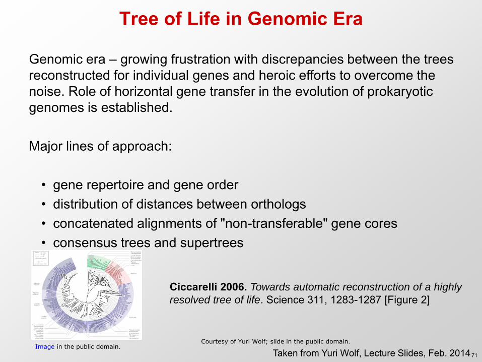
Genomic era – growing frustration with discrepancies between the trees reconstructed for individual genes and heroic efforts to overcome the noise. Role of horizontal gene transfer in the evolution of prokaryotic genomes is established. Major lines of approach:
• gene repertoire and gene order • distribution of distances between orthologs • concatenated alignments of "non-transferable" gene cores • consensus trees and supertrees
Ciccarelli 2006. Towards automatic reconstruction of a highly
resolved tree of life. Science 311, 1283-1287 [Figure 2]
Tree of Life in Genomic Era
Taken from Yuri Wolf, Lecture Slides, Feb. 2014 Image in the public domain.
Courtesy of Yuri Wolf; slide in the public domain.
71
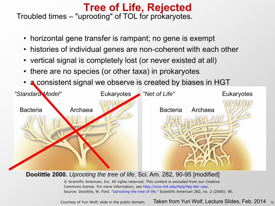
Doolittle 2000. Uprooting the tree of life. Sci. Am. 282, 90-95 [modified]
Tree of Life, Rejected
Bacteria Archaea
Eukaryotes
Bacteria Archaea
Eukaryotes
Troubled times – "uprooting" of TOL for prokaryotes.
• horizontal gene transfer is rampant; no gene is exempt • histories of individual genes are non-coherent with each other • vertical signal is completely lost (or never existed at all) • there are no species (or other taxa) in prokaryotes • a consistent signal we observe is created by biases in HGT
"Standard Model" "Net of Life"
Taken from Yuri Wolf, Lecture Slides, Feb. 2014
© Scientific American, Inc. All rights reserved. This content is excluded from our Creative
Commons license. For more information, see http://ocw.mit.edu/help/faq-fair-use/.
Source: Doolittle, W. Ford. "Uprooting the tree of life." Scientific American 282, no. 2 (2000): 90.
Courtesy of Yuri Wolf; slide in the public domain. 72
Forest of Life – Methods
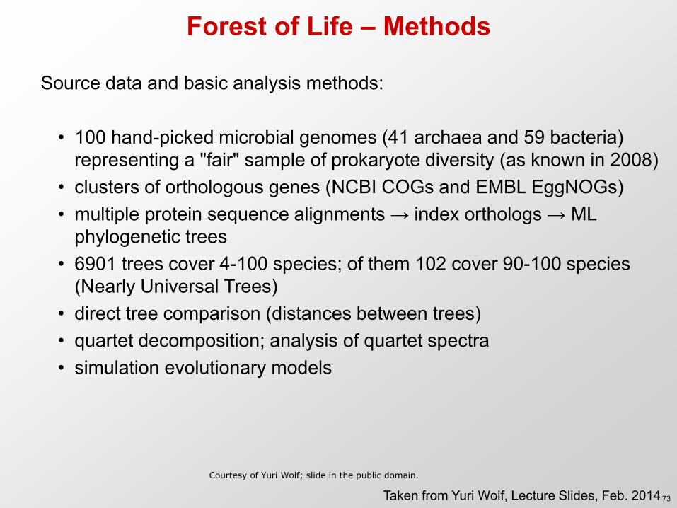
Source data and basic analysis methods:
• 100 hand-picked microbial genomes (41 archaea and 59 bacteria) representing a "fair" sample of prokaryote diversity (as known in 2008)
• clusters of orthologous genes (NCBI COGs and EMBL EggNOGs) • multiple protein sequence alignments → index orthologs → ML
phylogenetic trees • 6901 trees cover 4-100 species; of them 102 cover 90-100 species
(Nearly Universal Trees) • direct tree comparison (distances between trees) • quartet decomposition; analysis of quartet spectra • simulation evolutionary models
Taken from Yuri Wolf, Lecture Slides, Feb. 2014 Courtesy of Yuri Wolf; slide in the public domain.
73
Forest of Life – Analysis
0
0.5
1
CO
G0
54
1
CO
G0
53
2
CO
G0
09
2
CO
G0
10
0
CO
G0
09
0
CO
G0
52
8
CO
G0
09
6
CO
G0
52
5
CO
G0
05
1
CO
G0
45
2
CO
G0
49
5
CO
G0
17
2
CO
G0
08
9
CO
G0
52
2
CO
G0
12
4
CO
G0
18
5
CO
G0
09
4
CO
G0
12
6
CO
G0
51
9
CO
G0
54
0
CO
G0
14
9
CO
G0
19
8
CO
G0
17
7
CO
G0
05
7
CO
G0
00
9
CO
G0
53
7
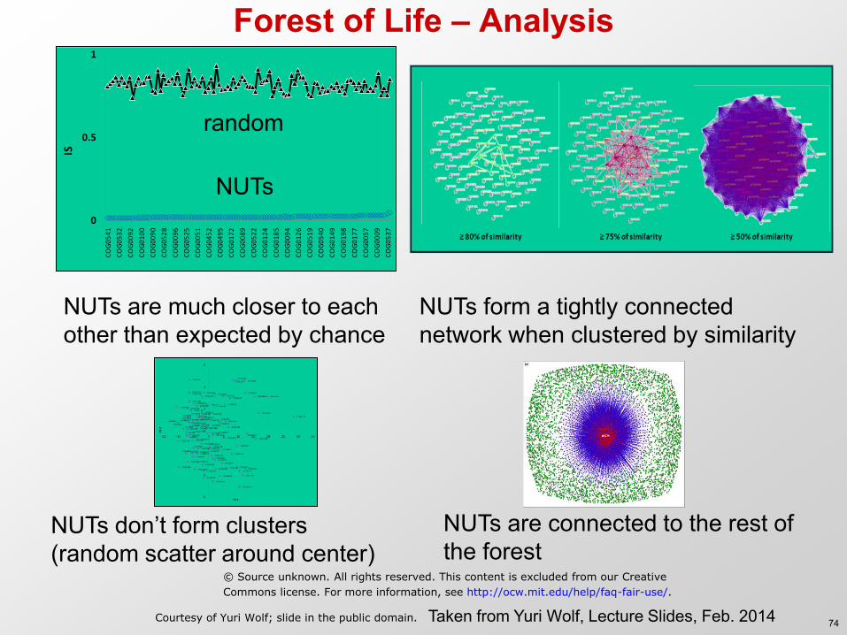
IS
NUTs
NUTs are much closer to each other than expected by chance
random
NUTs form a tightly connected network when clustered by similarity
NUTs don’t form clusters (random scatter around center)
NUTs are connected to the rest of the forest
Taken from Yuri Wolf, Lecture Slides, Feb. 2014
© Source unknown. All rights reserved. This content is excluded from our Creative
Commons license. For more information, see http://ocw.mit.edu/help/faq-fair-use/.
Courtesy of Yuri Wolf; slide in the public domain. 74
Forest of Life – Analysis
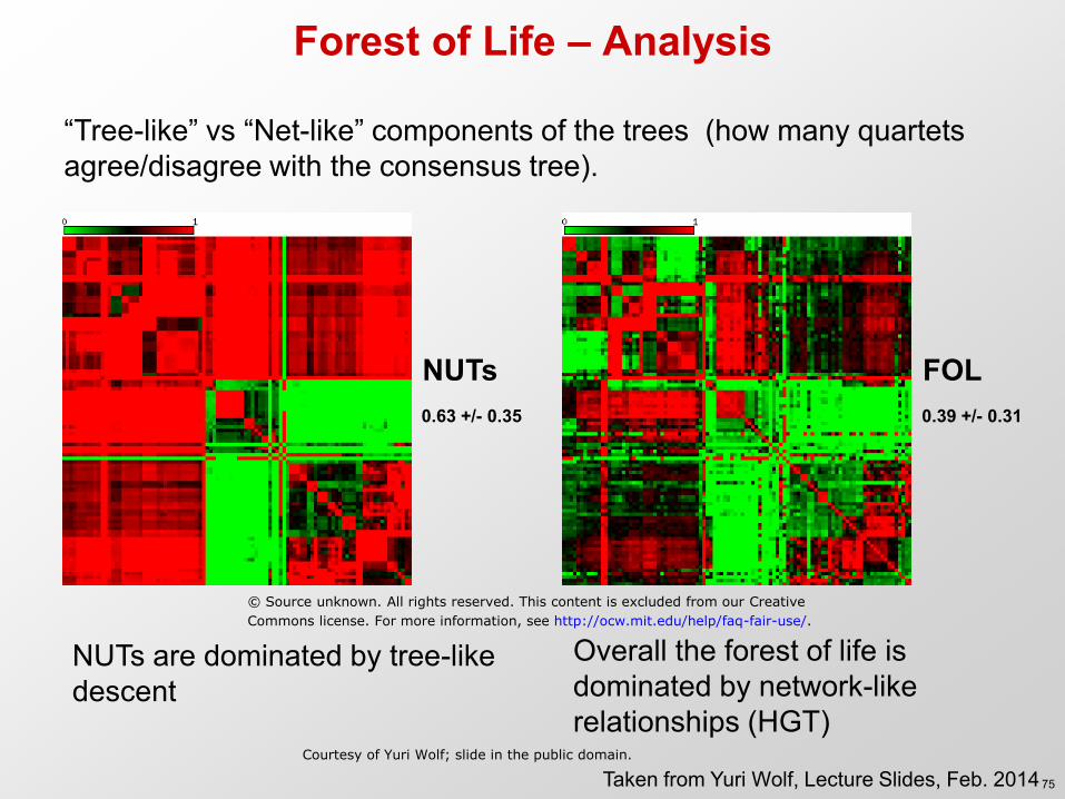
NUTs are dominated by tree-like descent
NUTs FOL 0.63 +/- 0.35 0.39 +/- 0.31
“Tree-like” vs “Net-like” components of the trees (how many quartets agree/disagree with the consensus tree).
Overall the forest of life is dominated by network-like relationships (HGT)
Taken from Yuri Wolf, Lecture Slides, Feb. 2014
© Source unknown. All rights reserved. This content is excluded from our Creative
Commons license. For more information, see http://ocw.mit.edu/help/faq-fair-use/.
Courtesy of Yuri Wolf; slide in the public domain.
75
Forest of Life – Analysis
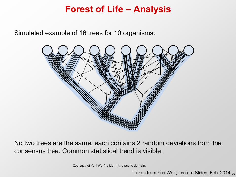
Simulated example of 16 trees for 10 organisms:
No two trees are the same; each contains 2 random deviations from the consensus tree. Common statistical trend is visible.
Taken from Yuri Wolf, Lecture Slides, Feb. 2014 Courtesy of Yuri Wolf; slide in the public domain.
76
Module V: Evolution/phylogeny/populations
• Phylogenetics / Phylogenomics – Phylogenetics: Evolutionary models, Tree building, Phylo inference – Phylogenomics: gene/species trees, reconciliation, coalescent, pops
• Population genomics: – Learning population history from genetic data – Assembling and getting information on genomes – Recitation about suffix arrays used in genome mapping and
assembly • Next Pset due on Nov 1st
– Don’t wait until the last week to start it! 77

MIT OpenCourseWarehttp://ocw.mit.edu
6.047 / 6.878 / HST.507 Computational BiologyFall 2015
For information about citing these materials or our Terms of Use, visit: http://ocw.mit.edu/terms.


![[MP] 02 - Phylogenetics - biologia.campusnet.unito.it · Molecular Phylogenetics Basis of Molecular Phylogenies Overview ¾Phylogenetics Definitions ¾Genetic Variation and Evolution](https://img.pdfslide.net/doc/110x75/5c6216d809d3f238158b4601/mp-02-phylogenetics-molecular-phylogenetics-basis-of-molecular-phylogenies.jpg)