Embed Size (px)
Citation preview
Lecture 7: Average value-at-risk
Prof. Dr. Svetlozar Rachev
Institute for Statistics and Mathematical EconomicsUniversity of Karlsruhe
Portfolio and Asset Liability Management
Summer Semester 2008
Prof. Dr. Svetlozar Rachev (University of Karlsruhe) Lecture 7: Average value-at-risk 2008 1 / 62
Copyright
These lecture-notes cannot be copied and/or distributed withoutpermission.The material is based on the text-book:Svetlozar T. Rachev, Stoyan Stoyanov, and Frank J. FabozziAdvanced Stochastic Models, Risk Assessment, and PortfolioOptimization: The Ideal Risk, Uncertainty, and PerformanceMeasuresJohn Wiley, Finance, 2007
Prof. Svetlozar (Zari) T. RachevChair of Econometrics, Statisticsand Mathematical FinanceSchool of Economics and Business EngineeringUniversity of KarlsruheKollegium am Schloss, Bau II, 20.12, R210Postfach 6980, D-76128, Karlsruhe, GermanyTel. +49-721-608-7535, +49-721-608-2042(s)Fax: +49-721-608-3811http://www.statistik.uni-karslruhe.de
Prof. Dr. Svetlozar Rachev (University of Karlsruhe) Lecture 7: Average value-at-risk 2008 2 / 62
Introduction
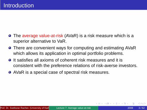
The average value-at-risk (AVaR) is a risk measure which is asuperior alternative to VaR.
There are convenient ways for computing and estimating AVaRwhich allows its application in optimal portfolio problems.
It satisfies all axioms of coherent risk measures and it isconsistent with the preference relations of risk-averse investors.
AVaR is a special case of spectral risk measures.
Prof. Dr. Svetlozar Rachev (University of Karlsruhe) Lecture 7: Average value-at-risk 2008 3 / 62
Average value-at-risk
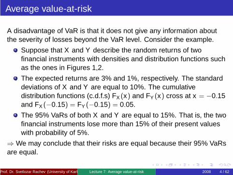
A disadvantage of VaR is that it does not give any information aboutthe severity of losses beyond the VaR level. Consider the example.
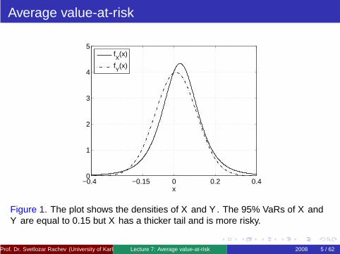
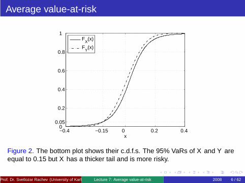
Suppose that X and Y describe the random returns of twofinancial instruments with densities and distribution functions suchas the ones in Figures 1,2.
The expected returns are 3% and 1%, respectively. The standarddeviations of X and Y are equal to 10%. The cumulativedistribution functions (c.d.f.s) FX (x) and FY (x) cross at x = −0.15and FX (−0.15) = FY (−0.15) = 0.05.
The 95% VaRs of both X and Y are equal to 15%. That is, the twofinancial instruments lose more than 15% of their present valueswith probability of 5%.
⇒ We may conclude that their risks are equal because their 95% VaRsare equal.
Prof. Dr. Svetlozar Rachev (University of Karlsruhe) Lecture 7: Average value-at-risk 2008 4 / 62
Average value-at-risk
−0.4 −0.15 0 0.2 0.40
1
2
3
4
5
x
fX(x)
fY(x)
Figure 1. The plot shows the densities of X and Y . The 95% VaRs of X andY are equal to 0.15 but X has a thicker tail and is more risky.
Prof. Dr. Svetlozar Rachev (University of Karlsruhe) Lecture 7: Average value-at-risk 2008 5 / 62
Average value-at-risk
−0.4 −0.15 0 0.2 0.4 0
0.05
0.2
0.4
0.6
0.8
1
x
FX(x)
FY(x)
Figure 2. The bottom plot shows their c.d.f.s. The 95% VaRs of X and Y areequal to 0.15 but X has a thicker tail and is more risky.
Prof. Dr. Svetlozar Rachev (University of Karlsruhe) Lecture 7: Average value-at-risk 2008 6 / 62
Average value-at-risk
The conclusion is wrong because we pay no attention to thelosses which are larger than the 95% VaR level.
It is visible in Figure 1 that the left tail of X is heavier than the lefttail of Y . It is more likely that the losses of X will be larger than thelosses of Y , on condition that they are larger than 15%.
Looking only at the losses occurring with probability smaller than5%, the random return X is riskier than Y .
If we base the analysis on the standard deviation and theexpected return, we would conclude that both X and Y have equalstandard deviations and X is actually preferable because of thehigher expected return.
In fact, we realize that it is exactly the opposite which shows howimportant it is to ground the reasoning on a proper risk measure.
Prof. Dr. Svetlozar Rachev (University of Karlsruhe) Lecture 7: Average value-at-risk 2008 7 / 62
Average value-at-risk
The disadvantage of VaR, that it is not informative about themagnitude of the losses larger than the VaR level, is not present inthe risk measure known as average value-at-risk.
In the literature, it is also called conditional value-at-risk orexpected shortfall but we will use average value-at-risk (AVaR) asit best describes the quantity it refers to.
Prof. Dr. Svetlozar Rachev (University of Karlsruhe) Lecture 7: Average value-at-risk 2008 8 / 62
Average value-at-risk
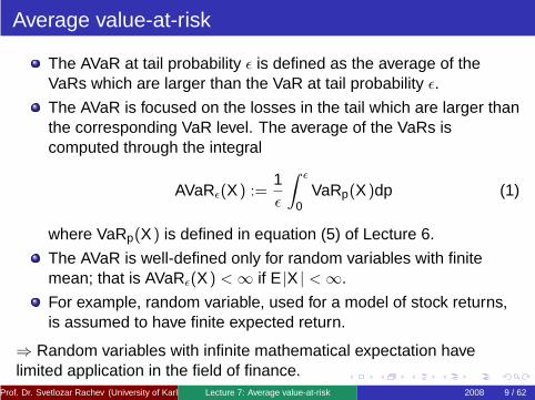
The AVaR at tail probability ǫ is defined as the average of theVaRs which are larger than the VaR at tail probability ǫ.
The AVaR is focused on the losses in the tail which are larger thanthe corresponding VaR level. The average of the VaRs iscomputed through the integral
AVaRǫ(X ) :=1ǫ
∫ ǫ
0VaRp(X )dp (1)
where VaRp(X ) is defined in equation (5) of Lecture 6.
The AVaR is well-defined only for random variables with finitemean; that is AVaRǫ(X ) < ∞ if E |X | < ∞.
For example, random variable, used for a model of stock returns,is assumed to have finite expected return.
⇒ Random variables with infinite mathematical expectation havelimited application in the field of finance.
Prof. Dr. Svetlozar Rachev (University of Karlsruhe) Lecture 7: Average value-at-risk 2008 9 / 62
Average value-at-risk
The AVaR satisfies all the axioms of coherent risk measures. It isconvex for all possible portfolios which means that it alwaysaccounts for the diversification effect.
A geometric interpretation of the definition in equation (1) isprovided in Figure 3, where the inverse c.d.f. of a r.v. X is plotted.
The shaded area is closed between the graph of F−1X (t) and the
horizontal axis for t ∈ [0, ǫ] where ǫ denotes the selected tailprobability.
AVaRǫ(X ) is the value for which the area of the drawn rectangle,equal to ǫ × AVaRǫ(X ), coincides with the shaded area which iscomputed by the integral in equation (1).
The VaRǫ(X ) value is always smaller than AVaRǫ(X ).
Prof. Dr. Svetlozar Rachev (University of Karlsruhe) Lecture 7: Average value-at-risk 2008 10 / 62
Average value-at-risk
0 0.15 0.4 0.6 0.8 1−0.6
−0.4
−0.2
0
0.2
0.4
t
F−1X
(t)
ε
AVaRε(X)
VaRε(X)
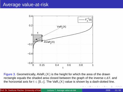
Figure 3. Geometrically, AVaRǫ(X ) is the height for which the area of the drawnrectangle equals the shaded area closed between the graph of the inverse c.d.f. andthe horizontal axis for t ∈ [0, ǫ]. The VaRǫ(X ) value is shown by a dash-dotted line.
Prof. Dr. Svetlozar Rachev (University of Karlsruhe) Lecture 7: Average value-at-risk 2008 11 / 62
Average value-at-risk
Recall the example with the VaRs at 5% tail probability, where wesaw that both random variables are equal. X is riskier than Ybecause the left tail of X is heavier than the left tail of Y ; that is,the distribution of X is more likely to produce larger losses thanthe distribution of Y on condition that the losses are beyond theVaR at the 5% tail probability.
We apply the geometric interpretation illustrated in Figure 3 to thisexample.
First, notice that the shaded area which concerns the graph of theinverse of the c.d.f. can also be identified through the graph of thec.d.f. (See the illustration in Figure 4).
Prof. Dr. Svetlozar Rachev (University of Karlsruhe) Lecture 7: Average value-at-risk 2008 12 / 62
Average value-at-risk
−0.4 −0.3 −0.1 0 0
0.05
0.1
0.15
0.2
FX(x)
FY(x)
AVaR0.05
(X)
AVaR0.05
(Y)
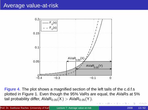
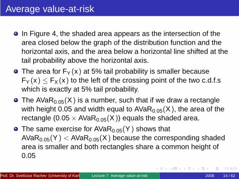
Figure 4. The plot shows a magnified section of the left tails of the c.d.f.splotted in Figure 1. Even though the 95% VaRs are equal, the AVaRs at 5%tail probability differ, AVaR0.05(X ) > AVaR0.05(Y ).
Prof. Dr. Svetlozar Rachev (University of Karlsruhe) Lecture 7: Average value-at-risk 2008 13 / 62
Average value-at-risk
In Figure 4, the shaded area appears as the intersection of thearea closed below the graph of the distribution function and thehorizontal axis, and the area below a horizontal line shifted at thetail probability above the horizontal axis.
The area for FY (x) at 5% tail probability is smaller becauseFY (x) ≤ FX (x) to the left of the crossing point of the two c.d.f.swhich is exactly at 5% tail probability.
The AVaR0.05(X ) is a number, such that if we draw a rectanglewith height 0.05 and width equal to AVaR0.05(X ), the area of therectangle (0.05 × AVaR0.05(X )) equals the shaded area.
The same exercise for AVaR0.05(Y ) shows thatAVaR0.05(Y ) < AVaR0.05(X ) because the corresponding shadedarea is smaller and both rectangles share a common height of0.05
Prof. Dr. Svetlozar Rachev (University of Karlsruhe) Lecture 7: Average value-at-risk 2008 14 / 62
Average value-at-risk
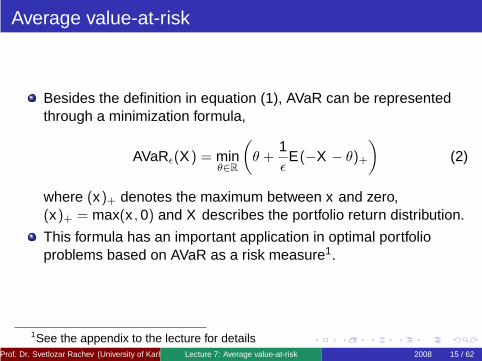
Besides the definition in equation (1), AVaR can be representedthrough a minimization formula,
AVaRǫ(X ) = minθ∈R
(
θ +1ǫ
E(−X − θ)+
)
(2)
where (x)+ denotes the maximum between x and zero,(x)+ = max(x , 0) and X describes the portfolio return distribution.
This formula has an important application in optimal portfolioproblems based on AVaR as a risk measure1.
1See the appendix to the lecture for detailsProf. Dr. Svetlozar Rachev (University of Karlsruhe) Lecture 7: Average value-at-risk 2008 15 / 62
Average value-at-risk
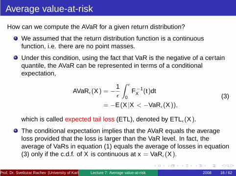
How can we compute the AVaR for a given return distribution?
We assumed that the return distribution function is a continuousfunction, i.e. there are no point masses.
Under this condition, using the fact that VaR is the negative of a certainquantile, the AVaR can be represented in terms of a conditionalexpectation,
AVaRǫ(X ) = −1ǫ
∫ ǫ
0F−1
X (t)dt
= −E(X |X < −VaRǫ(X )),
(3)
which is called expected tail loss (ETL), denoted by ETLǫ(X ).
The conditional expectation implies that the AVaR equals the averageloss provided that the loss is larger than the VaR level. In fact, theaverage of VaRs in equation (1) equals the average of losses in equation(3) only if the c.d.f. of X is continuous at x = VaRǫ(X ).
Prof. Dr. Svetlozar Rachev (University of Karlsruhe) Lecture 7: Average value-at-risk 2008 16 / 62
Average value-at-risk
Equation (3) implies that AVaR is related to the conditional lossdistribution.
If there is a discontinuity, or a point mass, the relationship is moreinvolved.
Under certain conditions, it is the mathematical expectation of theconditional loss distribution, which represents only onecharacteristic of it.
See the appendix to this lecture for several sets of characteristicsof the conditional loss distribution, which provide a more completepicture of it.
Prof. Dr. Svetlozar Rachev (University of Karlsruhe) Lecture 7: Average value-at-risk 2008 17 / 62
Average value-at-risk
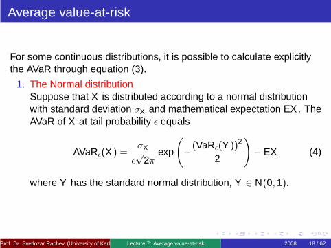
For some continuous distributions, it is possible to calculate explicitlythe AVaR through equation (3).
1. The Normal distributionSuppose that X is distributed according to a normal distributionwith standard deviation σX and mathematical expectation EX . TheAVaR of X at tail probability ǫ equals
AVaRǫ(X ) =σX
ǫ√
2πexp
(
−(VaRǫ(Y ))2
2
)
− EX (4)
where Y has the standard normal distribution, Y ∈ N(0, 1).
Prof. Dr. Svetlozar Rachev (University of Karlsruhe) Lecture 7: Average value-at-risk 2008 18 / 62
Average value-at-risk
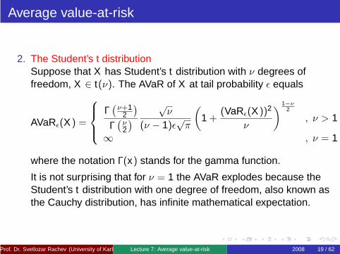
2. The Student’s t distributionSuppose that X has Student’s t distribution with ν degrees offreedom, X ∈ t(ν). The AVaR of X at tail probability ǫ equals
AVaRǫ(X ) =
Γ(
ν+12
)
Γ(
ν2
)
√ν
(ν − 1)ǫ√
π
(
1 +(VaRǫ(X ))2
ν
)
1−ν
2
, ν > 1
∞ , ν = 1
where the notation Γ(x) stands for the gamma function.
It is not surprising that for ν = 1 the AVaR explodes because theStudent’s t distribution with one degree of freedom, also known asthe Cauchy distribution, has infinite mathematical expectation.
Prof. Dr. Svetlozar Rachev (University of Karlsruhe) Lecture 7: Average value-at-risk 2008 19 / 62
Average value-at-risk
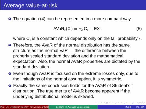
The equation (4) can be represented in a more compact way,
AVaRǫ(X ) = σX Cǫ − EX , (5)
where Cǫ is a constant which depends only on the tail probability ǫ.
Therefore, the AVaR of the normal distribution has the samestructure as the normal VaR — the difference between theproperly scaled standard deviation and the mathematicalexpectation. Also, the normal AVaR properties are dictated by thestandard deviation.
Even though AVaR is focused on the extreme losses only, due tothe limitations of the normal assumption, it is symmetric.
Exactly the same conclusion holds for the AVaR of Student’s tdistribution. The true merits of AVaR become apparent if theunderlying distributional model is skewed.
Prof. Dr. Svetlozar Rachev (University of Karlsruhe) Lecture 7: Average value-at-risk 2008 20 / 62
AVaR estimation from a sample
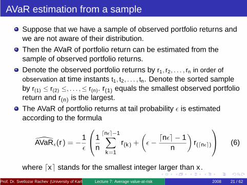
Suppose that we have a sample of observed portfolio returns andwe are not aware of their distribution.
Then the AVaR of portfolio return can be estimated from thesample of observed portfolio returns.
Denote the observed portfolio returns by r1, r2, . . . , rn in order ofobservation at time instants t1, t2, . . . , tn. Denote the sorted sampleby r(1) ≤ r(2) ≤, . . . ,≤ r(n). r(1) equals the smallest observed portfolioreturn and r(n) is the largest.
The AVaR of portfolio returns at tail probability ǫ is estimatedaccording to the formula
AVaRǫ(r) = −1ǫ
1n
⌈nǫ⌉−1∑
k=1
r(k) +
(
ǫ − ⌈nǫ⌉ − 1n
)
r(⌈nǫ⌉)
(6)
where ⌈x⌉ stands for the smallest integer larger than x .
Prof. Dr. Svetlozar Rachev (University of Karlsruhe) Lecture 7: Average value-at-risk 2008 21 / 62
AVaR estimation from a sample
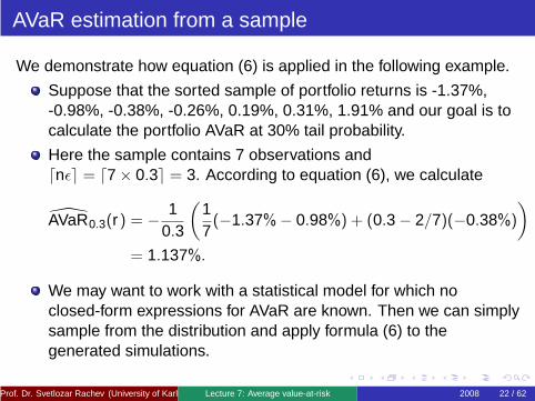
We demonstrate how equation (6) is applied in the following example.
Suppose that the sorted sample of portfolio returns is -1.37%,-0.98%, -0.38%, -0.26%, 0.19%, 0.31%, 1.91% and our goal is tocalculate the portfolio AVaR at 30% tail probability.
Here the sample contains 7 observations and⌈nǫ⌉ = ⌈7 × 0.3⌉ = 3. According to equation (6), we calculate
AVaR0.3(r) = − 10.3
(
17(−1.37% − 0.98%) + (0.3 − 2/7)(−0.38%)
)
= 1.137%.
We may want to work with a statistical model for which noclosed-form expressions for AVaR are known. Then we can simplysample from the distribution and apply formula (6) to thegenerated simulations.
Prof. Dr. Svetlozar Rachev (University of Karlsruhe) Lecture 7: Average value-at-risk 2008 22 / 62
AVaR estimation from a sample
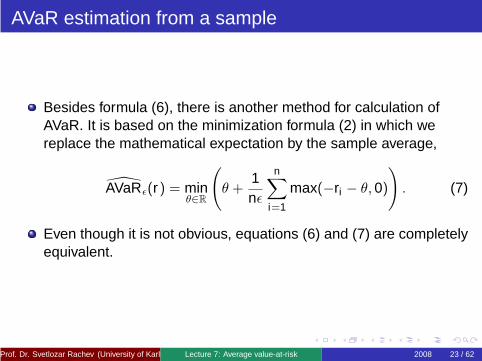
Besides formula (6), there is another method for calculation ofAVaR. It is based on the minimization formula (2) in which wereplace the mathematical expectation by the sample average,
AVaRǫ(r) = minθ∈R
(
θ +1nǫ
n∑
i=1
max(−ri − θ, 0)
)
. (7)
Even though it is not obvious, equations (6) and (7) are completelyequivalent.
Prof. Dr. Svetlozar Rachev (University of Karlsruhe) Lecture 7: Average value-at-risk 2008 23 / 62
AVaR estimation from a sample
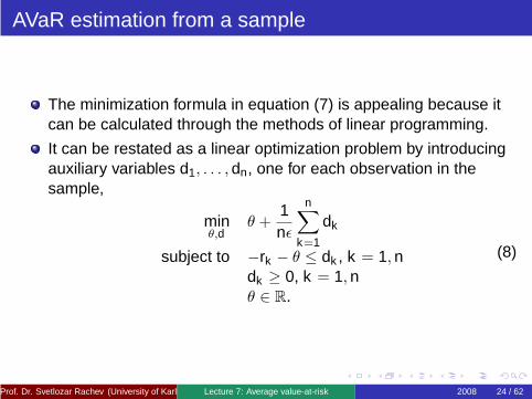
The minimization formula in equation (7) is appealing because itcan be calculated through the methods of linear programming.
It can be restated as a linear optimization problem by introducingauxiliary variables d1, . . . , dn, one for each observation in thesample,
minθ,d
θ +1nǫ
n∑
k=1
dk
subject to −rk − θ ≤ dk , k = 1, ndk ≥ 0, k = 1, nθ ∈ R.
(8)
Prof. Dr. Svetlozar Rachev (University of Karlsruhe) Lecture 7: Average value-at-risk 2008 24 / 62
AVaR estimation from a sample
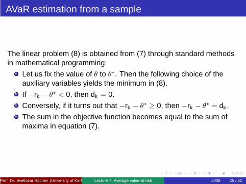
The linear problem (8) is obtained from (7) through standard methodsin mathematical programming:
Let us fix the value of θ to θ∗. Then the following choice of theauxiliary variables yields the minimum in (8).
If −rk − θ∗ < 0, then dk = 0.
Conversely, if it turns out that −rk − θ∗ ≥ 0, then −rk − θ∗ = dk .
The sum in the objective function becomes equal to the sum ofmaxima in equation (7).
Prof. Dr. Svetlozar Rachev (University of Karlsruhe) Lecture 7: Average value-at-risk 2008 25 / 62
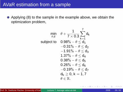
AVaR estimation from a sample
Applying (8) to the sample in the example above, we obtain theoptimization problem,
minθ,d
θ +1
7 × 0.3
7∑
k=1
dk
subject to 0.98% − θ ≤ d1
−0.31% − θ ≤ d2
−1.91% − θ ≤ d3
1.37% − θ ≤ d4
0.38% − θ ≤ d5
0.26% − θ ≤ d6
−0.19% − θ ≤ d7
dk ≥ 0, k = 1, 7θ ∈ R.
Prof. Dr. Svetlozar Rachev (University of Karlsruhe) Lecture 7: Average value-at-risk 2008 26 / 62
AVaR estimation from a sample
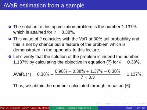
The solution to this optimization problem is the number 1.137%which is attained for θ = 0.38%.
This value of θ coincides with the VaR at 30% tail probability andthis is not by chance but a feature of the problem which isdemonstrated in the appendix to this lecture.
Let’s verify that the solution of the problem is indeed the number1.137% by calculating the objective in equation (7) for θ = 0.38%,
AVaRǫ(r) = 0.38% +0.98% − 0.38% + 1.37% − 0.38%
7 × 0.3= 1.137%.
Thus, we obtain the number calculated through equation (6).
Prof. Dr. Svetlozar Rachev (University of Karlsruhe) Lecture 7: Average value-at-risk 2008 27 / 62
Computing portfolio AVaR in practice
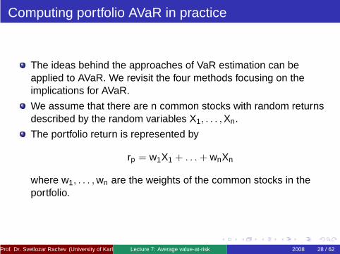
The ideas behind the approaches of VaR estimation can beapplied to AVaR. We revisit the four methods focusing on theimplications for AVaR.
We assume that there are n common stocks with random returnsdescribed by the random variables X1, . . . , Xn.
The portfolio return is represented by
rp = w1X1 + . . . + wnXn
where w1, . . . , wn are the weights of the common stocks in theportfolio.
Prof. Dr. Svetlozar Rachev (University of Karlsruhe) Lecture 7: Average value-at-risk 2008 28 / 62
The multivariate normal assumption
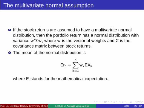
If the stock returns are assumed to have a multivariate normaldistribution, then the portfolio return has a normal distribution withvariance w ′Σw , where w is the vector of weights and Σ is thecovariance matrix between stock returns.
The mean of the normal distribution is
Erp =n∑
k=1
wkEXk
where E stands for the mathematical expectation.
Prof. Dr. Svetlozar Rachev (University of Karlsruhe) Lecture 7: Average value-at-risk 2008 29 / 62
The multivariate normal assumption
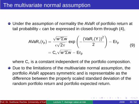
Under the assumption of normality the AVaR of portfolio return attail probability ǫ can be expressed in closed-form through (4),
AVaRǫ(rp) =
√w ′Σw
ǫ√
2πexp
(
−(VaRǫ(Y ))2
2
)
− Erp
= Cǫ
√w ′Σw − Erp
(9)
where Cǫ is a constant independent of the portfolio composition.
Due to the limitations of the multivariate normal assumption, theportfolio AVaR appears symmetric and is representable as thedifference between the properly scaled standard deviation of therandom portfolio return and portfolio expected return.
Prof. Dr. Svetlozar Rachev (University of Karlsruhe) Lecture 7: Average value-at-risk 2008 30 / 62
The Historical Method
The historical method is not related to any distributionalassumptions. We use the historically observed portfolio returns asa model for the future returns and apply formula (6) or (7).
We emphasize that the historical method is very inaccurate for lowtail probabilities, e.g. 1% or 5%.
Even with one year of daily returns which amounts to 250observations, in order to estimate the AVaR at 1% probability, wehave to use the 3 smallest observations which is quite insufficient.
What makes the estimation problem even worse is that theseobservations are in the tail of the distribution; that is, they are thesmallest ones in the sample.
The implication is that when the sample changes, the estimatedAVaR may change a lot because the smallest observations tend tofluctuate a lot.
Prof. Dr. Svetlozar Rachev (University of Karlsruhe) Lecture 7: Average value-at-risk 2008 31 / 62
The Hybrid Method
In the hybrid method, different weights are assigned to theobservations by which the more recent observations get a higherweight. The observations far back in the past have less impact onthe portfolio risk at the present time.
In AVaR estimation, the weights assigned to the observations areinterpreted as probabilities and the portfolio AVaR can beestimated from the resulting discrete distribution:
AVaRǫ(r) = −1ǫ
kǫ∑
j=1
pj r(j) +
ǫ −kǫ∑
j=1
pj
r(kǫ+1)
(10)
where r(1) ≤ r(2) ≤ . . . ≤ r(km) denotes the sorted sample ofportfolio returns or payoffs and p1, p2, . . . , pkm stand for theprobabilities of the sorted observations; that is, p1 is theprobability of r(1).
Prof. Dr. Svetlozar Rachev (University of Karlsruhe) Lecture 7: Average value-at-risk 2008 32 / 62
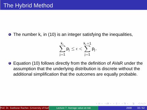
The Hybrid Method
The number kǫ in (10) is an integer satisfying the inequalities,
kǫ∑
j=1
pj ≤ ǫ <
kǫ+1∑
j=1
pj .
Equation (10) follows directly from the definition of AVaR under theassumption that the underlying distribution is discrete without theadditional simplification that the outcomes are equally probable.
Prof. Dr. Svetlozar Rachev (University of Karlsruhe) Lecture 7: Average value-at-risk 2008 33 / 62
The Monte Carlo Method
The basic steps of the Monte Carlo method, given in the previouslecture, are applied without modification.
We assume and estimate a multivariate statistical model for thestocks return distribution. Then we sample from it, and wecalculate scenarios for portfolio return.
On the basis of these scenarios, we estimate portfolio AVaR usingequation (6) in which r1, . . . , rn stands for the vector of generatedscenarios.
Prof. Dr. Svetlozar Rachev (University of Karlsruhe) Lecture 7: Average value-at-risk 2008 34 / 62
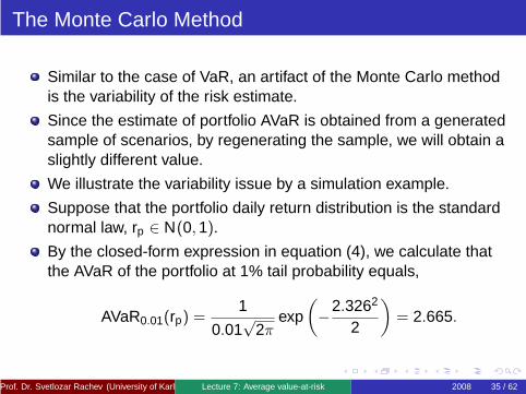
The Monte Carlo Method
Similar to the case of VaR, an artifact of the Monte Carlo methodis the variability of the risk estimate.
Since the estimate of portfolio AVaR is obtained from a generatedsample of scenarios, by regenerating the sample, we will obtain aslightly different value.
We illustrate the variability issue by a simulation example.
Suppose that the portfolio daily return distribution is the standardnormal law, rp ∈ N(0, 1).
By the closed-form expression in equation (4), we calculate thatthe AVaR of the portfolio at 1% tail probability equals,
AVaR0.01(rp) =1
0.01√
2πexp
(
−2.3262
2
)
= 2.665.
Prof. Dr. Svetlozar Rachev (University of Karlsruhe) Lecture 7: Average value-at-risk 2008 35 / 62
The Monte Carlo Method
In order to investigate how the fluctuations of the 99% AVaRchange about the theoretical value, we generate samples ofdifferent sizes: 500, 1,000, 5,000, 10,000, 20,000, and 100,000scenarios.
The 99% AVaR is computed from these samples using equation(6) and the numbers are stored.
We repeat the experiment 100 times. In the end, we have 100AVaR numbers for each sample size. We expect that as thesample size increases, the AVaR values will fluctuate less aboutthe theoretical value which is AVaR0.01(X ) = 2.665, X ∈ N(0, 1).
Prof. Dr. Svetlozar Rachev (University of Karlsruhe) Lecture 7: Average value-at-risk 2008 36 / 62
The Monte Carlo Method
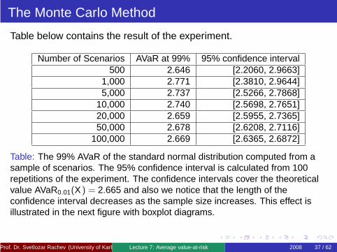
Table below contains the result of the experiment.
Number of Scenarios AVaR at 99% 95% confidence interval500 2.646 [2.2060, 2.9663]
1,000 2.771 [2.3810, 2.9644]5,000 2.737 [2.5266, 2.7868]
10,000 2.740 [2.5698, 2.7651]20,000 2.659 [2.5955, 2.7365]50,000 2.678 [2.6208, 2.7116]
100,000 2.669 [2.6365, 2.6872]
Table: The 99% AVaR of the standard normal distribution computed from asample of scenarios. The 95% confidence interval is calculated from 100repetitions of the experiment. The confidence intervals cover the theoreticalvalue AVaR0.01(X ) = 2.665 and also we notice that the length of theconfidence interval decreases as the sample size increases. This effect isillustrated in the next figure with boxplot diagrams.
Prof. Dr. Svetlozar Rachev (University of Karlsruhe) Lecture 7: Average value-at-risk 2008 37 / 62
The Monte Carlo Method
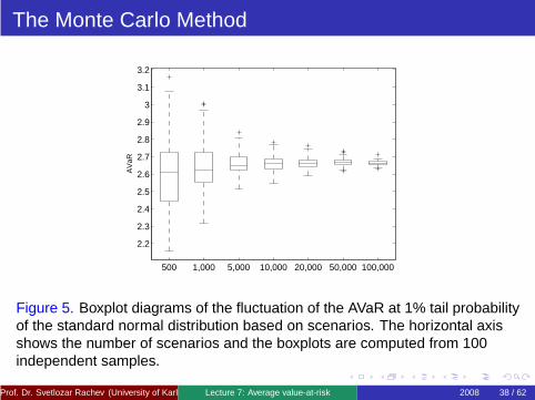
500 1,000 5,000 10,000 20,000 50,000 100,000
2.2
2.3
2.4
2.5
2.6
2.7
2.8
2.9
3
3.1
3.2
AV
aR
Figure 5. Boxplot diagrams of the fluctuation of the AVaR at 1% tail probabilityof the standard normal distribution based on scenarios. The horizontal axisshows the number of scenarios and the boxplots are computed from 100independent samples.
Prof. Dr. Svetlozar Rachev (University of Karlsruhe) Lecture 7: Average value-at-risk 2008 38 / 62
The Monte Carlo Method
A sample of 100,000 scenarios results in AVaR numbers whichare tightly packed around the true value. A sample of only 500scenarios may give a very inaccurate estimate.
By comparing the given table to table (VaR computation) on theslide 62 in lecture 6, we notice that the length of the 95%confidence intervals for AVaR are larger than the correspondingconfidence intervals for VaR.
Given that both quantities are at the same tail probability of 1%,the AVaR has larger variability than the VaR for a fixed number ofscenarios because the AVaR is the average of terms fluctuatingmore than the 1% VaR.
This effect is more pronounced the more heavy-tailed thedistribution is.
Prof. Dr. Svetlozar Rachev (University of Karlsruhe) Lecture 7: Average value-at-risk 2008 39 / 62
Back-testing of AVaR
How we can verify if the estimates of daily AVaR are realistic?
In the context of VaR, a back-testing was used. It consists of computingthe portfolio VaR for each day back in time using the informationavailable up to that day only.
On the basis of the VaR numbers back in time and the realized portfolioreturns, we can use statistical methods to assess whether the forecastedloss at the VaR tail probability is consistent with the observed losses.
If there are too many observed losses larger than the forecasted VaR,then the model is too optimistic.
If there are too few losses larger than the forecasted VaR, then themodel is too pessimistic.
In this case we are simply counting the cases in which there is anexceedance.
Prof. Dr. Svetlozar Rachev (University of Karlsruhe) Lecture 7: Average value-at-risk 2008 40 / 62
Back-testing of AVaR
Back-testing of AVaR is not so straightforward.
By definition, the AVaR at tail probability ǫ is the average of VaRs largerthan the VaR at tail probability ǫ.
The most direct approach to test AVaR would be to perform VaRback-tests at all tail probabilities smaller than ǫ. If all these VaRs arecorrectly modeled, then so is the corresponding AVaR.
⇒ But it is impossible to perform in practice.
Suppose that we consider the AVaR at tail probability of 1%, forexample. Back-testing VaRs deeper in the tail of the distribution can beinfeasible because the back-testing time window is too short.
The lower the tail probability, the larger time window we need in order forthe VaR test to be conclusive.
Even if the VaR back-testing fails at some tail probability ǫ1 below ǫ, thisdoes not necessarily mean that the AVaR is incorrectly modeledbecause the test failure may be due to purely statistical reasons and notto incorrect modeling.
Prof. Dr. Svetlozar Rachev (University of Karlsruhe) Lecture 7: Average value-at-risk 2008 41 / 62
Back-testing of AVaR
Why AVaR back-testing is a difficult problem?
We need the information about the entire tail of the returndistribution describing the losses larger than the VaR at tailprobability ǫ and there may be too few observations from the tailupon which to base the analysis.
For example, in one business year, there are typically 250 tradingdays. Therefore, a one-year back-testing results in 250 dailyportfolio returns which means that if ǫ = 1%, then there are only 2observations available from the losses larger than the VaR at 1%tail probability.
Prof. Dr. Svetlozar Rachev (University of Karlsruhe) Lecture 7: Average value-at-risk 2008 42 / 62
Back-testing of AVaR
As a result, in order to be able to back-test AVaR, we can assume acertain “structure” of the tail of the return distribution which wouldcompensate for the lack of observations.
There are two general approaches:
1. Use the tails of the Lévy stable distributions as a proxy for the tailof the loss distribution and take advantage of the practicalsemi-analytic formula for the AVaR2.
2. Make the weaker assumption that the loss distribution belongs tothe domain of attraction of a max-stable distribution. Thus, thebehavior of the large losses can be approximately described bythe limit max-stable distribution and a statistical test can be basedon it.
2See the appendix.Prof. Dr. Svetlozar Rachev (University of Karlsruhe) Lecture 7: Average value-at-risk 2008 43 / 62
Back-testing of AVaR
The rationale of the first approach:
Generally, the Lévy stable distribution provides a good fit to the stockreturns data and, thus, the stable tail may turn out to be a reasonableapproximation.
From the Generalized central limit theorem we know that stabledistributions have domains of attraction which makes them an appealingcandidate for an approximate model.
The second approach is based on a weaker assumption:
The family of max-stable distributions arises as the limit distribution ofproperly scaled and centered maxima of i.i.d. random variables.
If the random variable describes portfolio losses, then the limitmax-stable distribution can be used as a model for the large losses.
But then the estimators of poor quality have to be used to estimate theparameters of the limit max-stable distribution, such as the Hill estimatorfor example. This represents the basic trade-off in this approach.
Prof. Dr. Svetlozar Rachev (University of Karlsruhe) Lecture 7: Average value-at-risk 2008 44 / 62
Spectral risk measures
By definition, the AVaR at tail probability ǫ is the average of theVaRs larger than the VaR at tail probability ǫ.
It appears possible to obtain a larger family of coherent riskmeasures by considering the weighted average of the VaRsinstead of simple average.
Thus, the AVaR becomes just one representative of this largerfamily which is known as spectral risk measures.
Prof. Dr. Svetlozar Rachev (University of Karlsruhe) Lecture 7: Average value-at-risk 2008 45 / 62
Spectral risk measures
Spectral risk measures are defined as,3
ρφ(X ) =
∫ 1
0VaRp(X )φ(p)dp (11)
where φ(p), p ∈ [0, 1] is the weighting function also known as riskspectrum or risk-aversion function.
It has the following interpretation. Consider a small interval [p1, p2]of tail probabilities with length p2 − p1 = ∆p. The weightcorresponding to this interval is approximately equal toφ(p1) × ∆p.
Thus, the VaRs at tail probabilities belonging to this interval haveapproximately the weight φ(p1) × ∆p.
3See Acerbi(2004) for further details.Prof. Dr. Svetlozar Rachev (University of Karlsruhe) Lecture 7: Average value-at-risk 2008 46 / 62
Spectral risk measures
The risk-aversion function should possess some properties in order forρφ(X ) to be a coherent risk measure, it should be:
Positive φ(p) ≥ 0, p ∈ [0, 1].
Non-increasing Larger losses are multiplied by largerweights, φ(p1) ≥ φ(p2), p1 ≤ p2.
Normed All weights should sum up to 1,∫ 1
0 φ(p)dp = 1.
If we compare equations (11) and (1) we notice that the AVaR at tailprobability ǫ arises from a spectral risk measure with a constant riskaversion function for all tail probabilities below ǫ.
Prof. Dr. Svetlozar Rachev (University of Karlsruhe) Lecture 7: Average value-at-risk 2008 47 / 62
Spectral risk measures
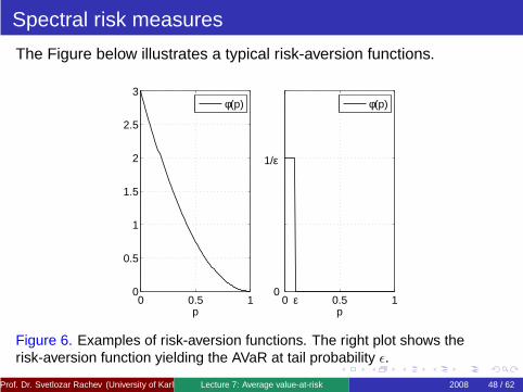
The Figure below illustrates a typical risk-aversion functions.
0 0.5 10
0.5
1
1.5
2
2.5
3
p
0 0.5 10
p
φ(p)φ(p)
ε
1/ε
Figure 6. Examples of risk-aversion functions. The right plot shows therisk-aversion function yielding the AVaR at tail probability ǫ.
Prof. Dr. Svetlozar Rachev (University of Karlsruhe) Lecture 7: Average value-at-risk 2008 48 / 62
Spectral risk measures
In the part of AVaR computation we emphasized that if a sample isused to estimate VaR and AVaR, then there is certain variability ofthe estimates. We illustrated it through a Monte Carlo example forthe standard normal distribution.
Comparing the results we concluded that the variability of AVaR islarger than the VaR at the same tail probability because in theAVaR, we average terms with larger variability. The heavier thetail, the more pronounced this effect becomes.
Prof. Dr. Svetlozar Rachev (University of Karlsruhe) Lecture 7: Average value-at-risk 2008 49 / 62
Spectral risk measures
When spectral risk measures are estimated from a sample, thevariability of the estimate may become a big issue.
Note that due to the non-increasing property of the risk-aversionfunction, the larger losses, which are deeper in the tail of thereturn distribution, are multiplied by a larger weight.
The larger losses (VaRs at lower tail probability) have highervariability and the multiplication by a larger weight furtherincreases the variability of the weighted average.
Therefore, larger number of scenarios may turn out to benecessary to achieve given stability of the estimate for spectralrisk measures than for AVaR.
Prof. Dr. Svetlozar Rachev (University of Karlsruhe) Lecture 7: Average value-at-risk 2008 50 / 62
Spectral risk measures
The distributional assumption for the r.v. X is very importantbecause it may lead to unbounded spectral risk measures forsome choices of the risk-aversion function.
An infinite risk measure is not informative for decision makers andan unfortunate combination of a distributional model and arisk-aversion function cannot be identified by looking at thesample estimate of ρφ(X ).
In practice, when ρφ(X ) is divergent in theory, we will observe highvariability of the risk estimates when regenerating the simulationsand also non-decreasing variability of the risk estimates as weincrease the number of simulations.
Prof. Dr. Svetlozar Rachev (University of Karlsruhe) Lecture 7: Average value-at-risk 2008 51 / 62
Spectral risk measures
We would like to stress that this problem does not exist for AVaRbecause a finite mean of X guarantees that the AVaR is welldefined on all tail probability levels.
The problem for the spectral measures of risk arises from thenon-increasing property of the risk-aversion function. Largerlosses are multiplied by larger weights which may result in anunbounded weighted average.
Prof. Dr. Svetlozar Rachev (University of Karlsruhe) Lecture 7: Average value-at-risk 2008 52 / 62
Risk measures and probability metrics
The probability metrics provide the only way of measuring distancesbetween random quantities.
A small distance between random quantities does not necessarily implythat selected characteristics of those quantities will be close to eachother.
For example, a probability metric may indicate that two distributions areclose to each other and, still, the standard deviations of the twodistributions may be arbitrarily different.
As a very extreme case, one of the distributions may even have aninfinite standard deviation.
If we want small distances measured by a probability metric to implysimilar characteristics, the probability metric should be carefully chosen.
A small distance between 2 random quantities estimated by an idealmetric means that the 2 random variables have similar absolutemoments.
Prof. Dr. Svetlozar Rachev (University of Karlsruhe) Lecture 7: Average value-at-risk 2008 53 / 62
Risk measures and probability metrics
A risk measure can be viewed as calculating a particular characteristicof a random variable.
There are problems in finance in which the goal is to find a randomvariable closest to another random variable. For instance, such is thebenchmark tracking problem which is at the heart of passive portfolioconstruction strategies.
Essentially, we are trying to construct a portfolio tracking theperformance a given benchmark; that is finding a portfolio returndistribution which is closest to the return distribution of the benchmark.
Usually, the distance is measured through the tracking error which is thestandard deviation of the active return.
Prof. Dr. Svetlozar Rachev (University of Karlsruhe) Lecture 7: Average value-at-risk 2008 54 / 62
Risk measures and probability metrics
Suppose that we have found the portfolio tracking the benchmark mostclosely with respect to the tracking error.Can we be sure that the risk of the portfolio is close to the risk of thebenchmark?
Generally, the answer is affirmative only if we use the standard deviationas a risk measure.
Active return is refined as the difference between the portfolio return rp
and the benchmark return rb, rp − rb. The conclusion that smallertracking error implies that the standard deviation of rp is close to thestandard deviation of rb is based on the inequality,
|σ(rp) − σ(rb)| ≤ σ(rp − rb).
The right part corresponds to the tracking error and, therefore, smallertracking error results in σ(rp) being closer to σ(rb).
Prof. Dr. Svetlozar Rachev (University of Karlsruhe) Lecture 7: Average value-at-risk 2008 55 / 62
Risk measures and probability metrics
In order to guarantee that small distance between portfolio returndistributions corresponds to similar risks, we have to find a suitableprobability metric.
Technically, for a given risk measure we need to find a probability metricwith respect to which the risk measure is a continuous functional,
|ρ(X ) − ρ(Y )| ≤ µ(X , Y ),
where ρ is the risk measure and µ stands for the probability metric.
We continue with examples of how this can be done for VaR, AVaR, andthe spectral risk measures.
Prof. Dr. Svetlozar Rachev (University of Karlsruhe) Lecture 7: Average value-at-risk 2008 56 / 62
Risk measures and probability metrics
1. VaRSuppose that X and Y describe the return distributions of two portfolios.The absolute difference between the VaRs of the two portfolios at anytail probability can be bounded by,
|VaRǫ(X ) − VaRǫ(Y )| ≤ maxp∈(0,1)
|VaRp(X ) − VaRp(Y )|
= maxp∈(0,1)
|F−1Y (p) − F−1
X (p)|
= W(X , Y )
where W(X , Y ) is the uniform metric between inverse distributionfunctions.
If the distance between X and Y is small, as measured by the metricW(X , Y ), then the VaR of X is close to the VaR of Y at any tailprobability level ǫ.
Prof. Dr. Svetlozar Rachev (University of Karlsruhe) Lecture 7: Average value-at-risk 2008 57 / 62
Risk measures and probability metrics
2. AVaRSuppose that X and Y describe the return distributions of two portfolios.The absolute difference between the AVaRs of the two portfolios at anytail probability can be bounded by,
|AVaRǫ(X ) − AVaRǫ(Y )| ≤ 1ǫ
∫ ǫ
0|F−1
X (p) − F−1Y (p)|dp
≤∫ 1
0|F−1
X (p) − F−1Y (p)|dp
= κ(X , Y )
where κ(X , Y ) is the Kantorovich metric.
If the distance between X and Y is small, as measured by the metricκ(X , Y ), then the AVaR of X is close to the AVaR of Y at any tailprobability level ǫ.
Prof. Dr. Svetlozar Rachev (University of Karlsruhe) Lecture 7: Average value-at-risk 2008 58 / 62
Risk measures and probability metrics
Note that the quantity
κǫ(X , Y ) =1ǫ
∫ ǫ
0|F−1
X (p) − F−1Y (p)|dp
can also be used to bound the absolute difference between the AVaRs.
It is a probability semi-metric giving the best possible upper bound on theabsolute difference between the AVaRs.
Prof. Dr. Svetlozar Rachev (University of Karlsruhe) Lecture 7: Average value-at-risk 2008 59 / 62
Risk measures and probability metrics
3. Spectral risk measuresSuppose that X and Y describe the return distributions of two portfolios.The absolute difference between the spectral risk measures of the twoportfolios for a given risk-aversion function can be bounded by,
|ρφ(X ) − ρφ(Y )| ≤∫ 1
0|F−1
X (p) − F−1Y (p)|φ(p)dp
= κφ(X , Y )
where κφ(X , Y ) is a weighted Kantorovich metric.
If the distance between X and Y is small, as measured by the metricκφ(X , Y ), then the risk of X is close to the risk of Y as measured by thespectral risk measure ρφ.
Prof. Dr. Svetlozar Rachev (University of Karlsruhe) Lecture 7: Average value-at-risk 2008 60 / 62
Summary
We considered in detail the AVaR risk measure. We noted theadvantages of AVaR, described a number of methods for its calculationand estimation, and remarked some potential pitfalls including estimatesvariability and problems on AVaR back-testing. We illustratedgeometrically many of the formulae for AVaR calculation, which makesthem more intuitive and easy to understand.
We also considered a more general family of coherent risk measures —the spectral risk measures. The AVaR is a spectral risk measure with aspecific risk-aversion function. We emphasized the importance of properselection of the risk-aversion function to avoid explosion of the riskmeasure.
Finally, we demonstrated a connection between the theory of probabilitymetrics and risk measures. Basically, by choosing an appropriateprobability metric we can guarantee that if two portfolio returndistributions are close to each other, their risk profiles are also similar.
Prof. Dr. Svetlozar Rachev (University of Karlsruhe) Lecture 7: Average value-at-risk 2008 61 / 62
Svetlozar T. Rachev, Stoyan Stoyanov, and Frank J. Fabozzi
Advanced Stochastic Models, Risk Assessment, and PortfolioOptimization: The Ideal Risk, Uncertainty, and Performance MeasuresJohn Wiley, Finance, 2007.
Chapter 7.
Prof. Dr. Svetlozar Rachev (University of Karlsruhe) Lecture 7: Average value-at-risk 2008 62 / 62