Lecture 7 Overview - University of Otago · Lecture 7 Overview • Last Lecture ... • Routing protocol design in Contiki – Communication architecture in Contiki – Rime communication

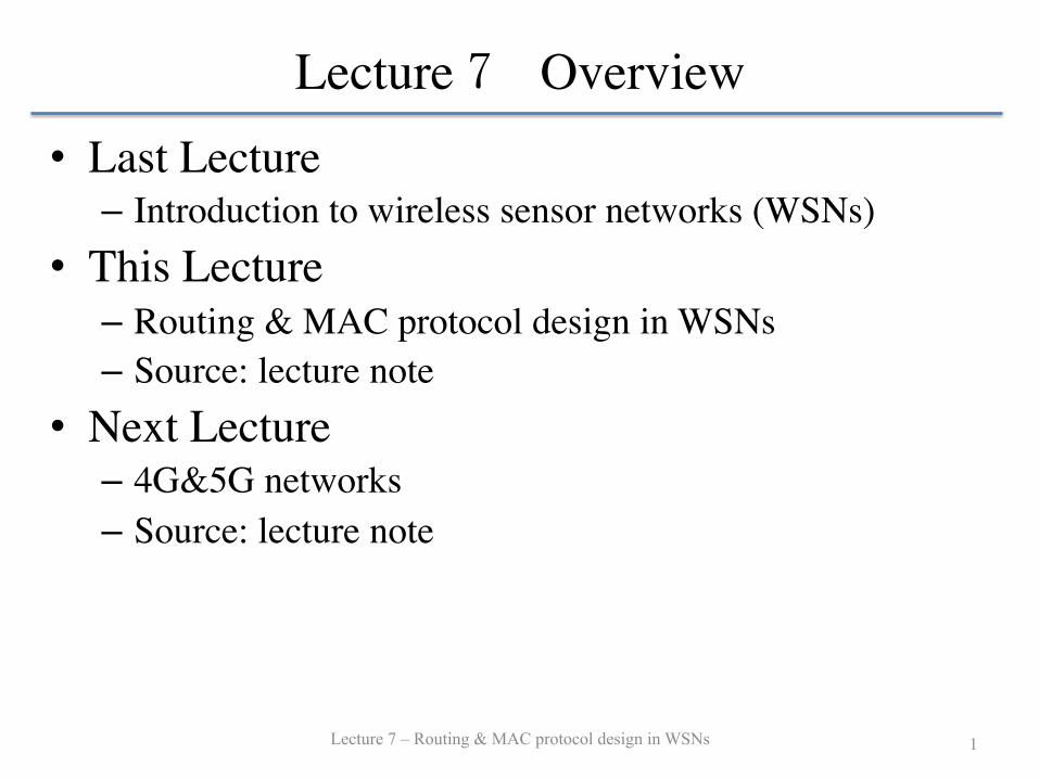
Lecture 7 Overview•  Last Lecture

–  Introduction to wireless sensor networks (WSNs)•  This Lecture

– Routing & MAC protocol design in WSNs–  Source: lecture note

•  Next Lecture–  4G&5G networks–  Source: lecture note

Lecture 7 – Routing & MAC protocol design in WSNs 1

Roadmap•  Routing protocols for WSNs

– Design challenges– Energy-aware routing – Hierarchical routing – Geographic routing– Graph routing

•  Routing protocol design in Contiki– Communication architecture in Contiki– Rime communication stack


Routing in WSNs


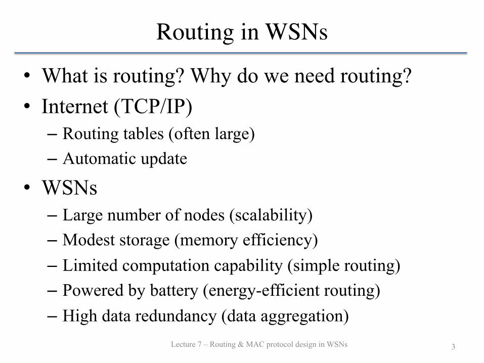
•  What is routing? Why do we need routing? •  Internet (TCP/IP)

– Routing tables (often large) – Automatic update

•  WSNs – Large number of nodes (scalability) – Modest storage (memory efficiency) – Limited computation capability (simple routing) –  Powered by battery (energy-efficient routing) – High data redundancy (data aggregation)

Routing Metrics


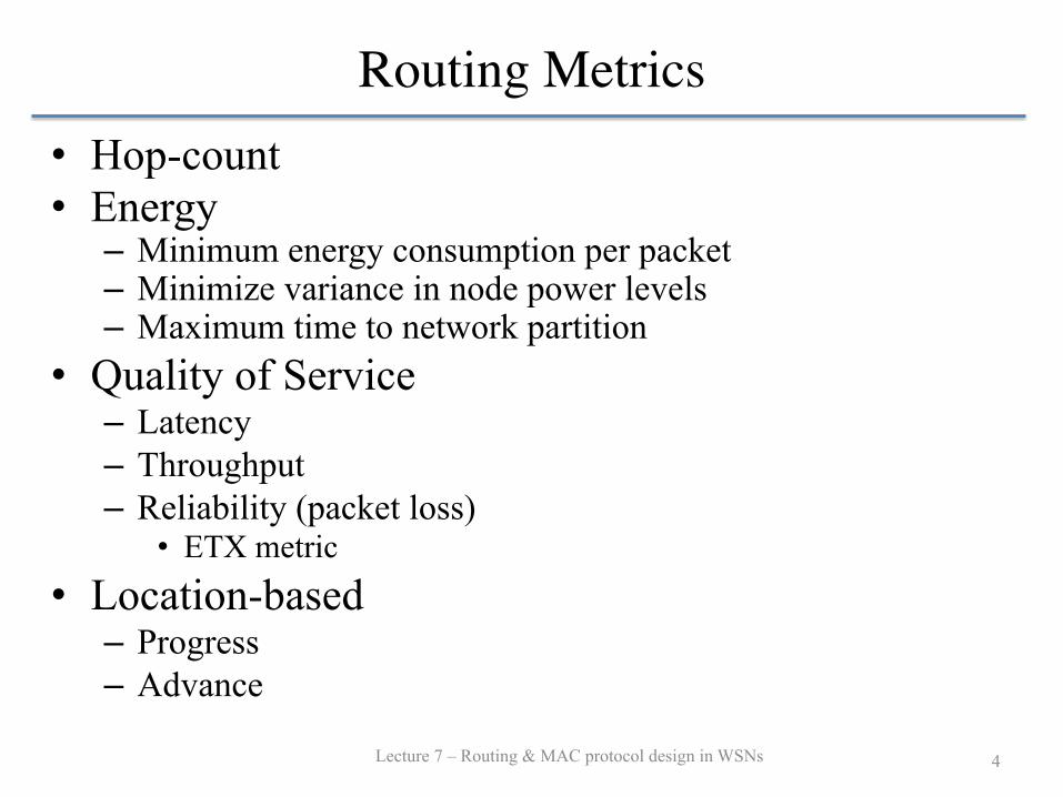
•  Hop-count •  Energy

–  Minimum energy consumption per packet –  Minimize variance in node power levels –  Maximum time to network partition

•  Quality of Service –  Latency –  Throughput –  Reliability (packet loss)

•  ETX metric •  Location-based

–  Progress –  Advance

Energy-efficient routing


•  Number along links: energy for transmission over link •  Number in parentheses: remaining energy capacity

n  Minimum hop: S-B-I-O (13) n  Minimum energy: S-A-D-F-I-O (9) n  Maximum minimum residual energy: S-C-E-H-G-I-O (16)

A

B

C

D

E

F

G

H

I

J

K

(5)(4)

(6)

(5)(3)

(3)

(4) (1) (5) (4)

(3)

2

1

2 12

2

1

4

35

2 2

1

3

3

3

3

42

4

34

SO

8

Energy-efficient routing (cont.)


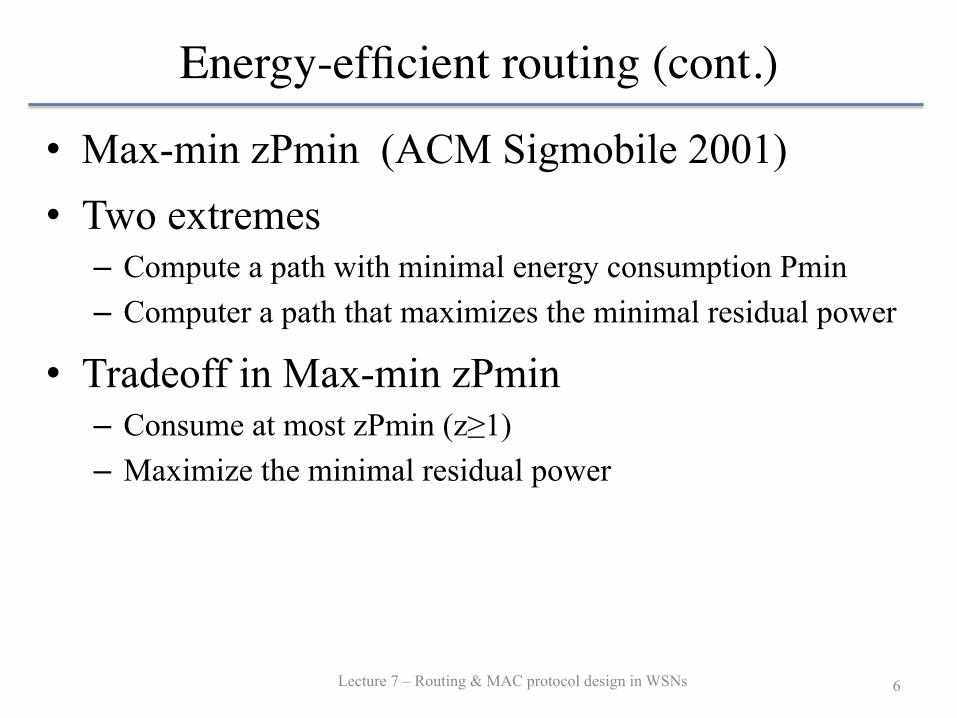
•  Max-min zPmin (ACM Sigmobile 2001) •  Two extremes

–  Compute a path with minimal energy consumption Pmin –  Computer a path that maximizes the minimal residual power

•  Tradeoff in Max-min zPmin –  Consume at most zPmin (z≥1) –  Maximize the minimal residual power

Energy-efficient routing (cont.)

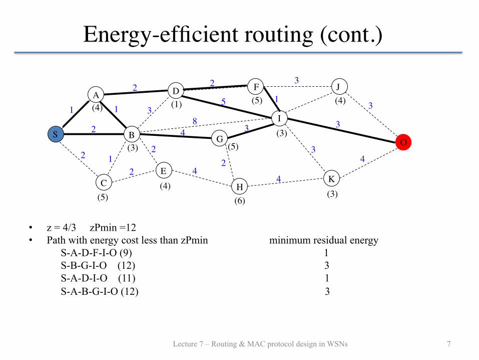
•  z = 4/3 zPmin =12 •  Path with energy cost less than zPmin minimum residual energy S-A-D-F-I-O (9) 1 S-B-G-I-O (12) 3 S-A-D-I-O (11) 1 S-A-B-G-I-O (12) 3

A

B

C

D

E

F

G

H

I

J

K

(5)(4)

(6)

(5)(3)

(3)

(4) (1) (5) (4)

(3)

2

1

2 12

2

1

4

35

2 2

1

3

3

3

3

42

4

34

SO

8


Hierarchical Routing

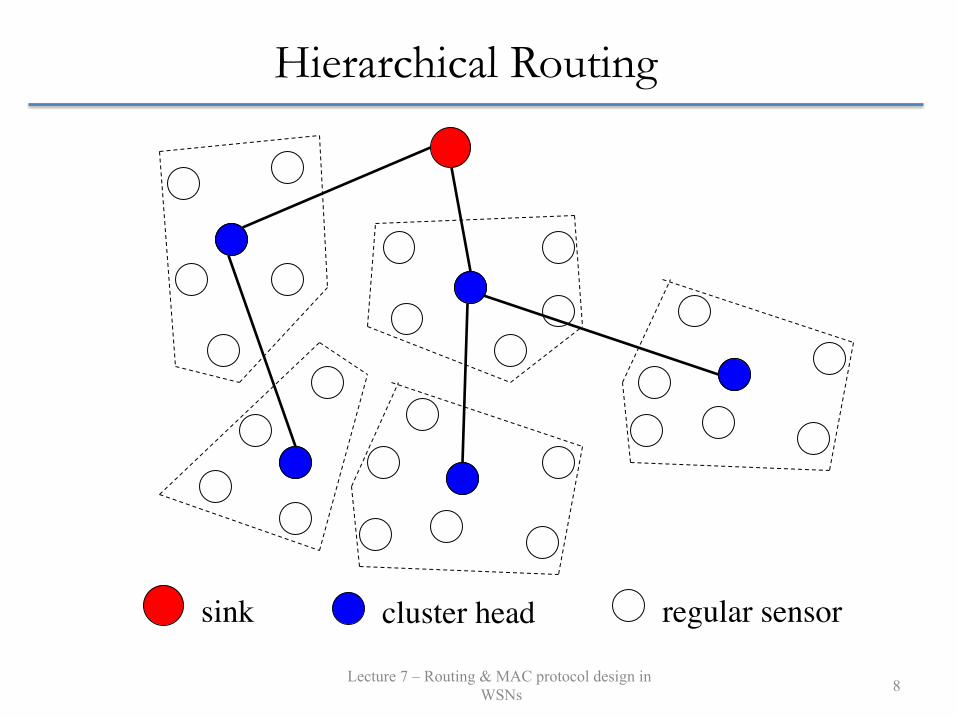
sink cluster head regular sensor


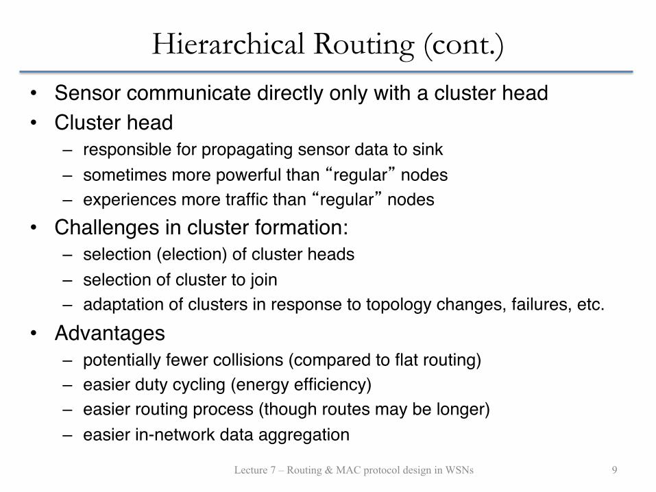
Hierarchical Routing (cont.) •  Sensor communicate directly only with a cluster head•  Cluster head

–  responsible for propagating sensor data to sink–  sometimes more powerful than “regular” nodes–  experiences more traffic than “regular” nodes

•  Challenges in cluster formation:–  selection (election) of cluster heads–  selection of cluster to join–  adaptation of clusters in response to topology changes, failures, etc.

•  Advantages–  potentially fewer collisions (compared to flat routing)–  easier duty cycling (energy efficiency)–  easier routing process (though routes may be longer)–  easier in-network data aggregation


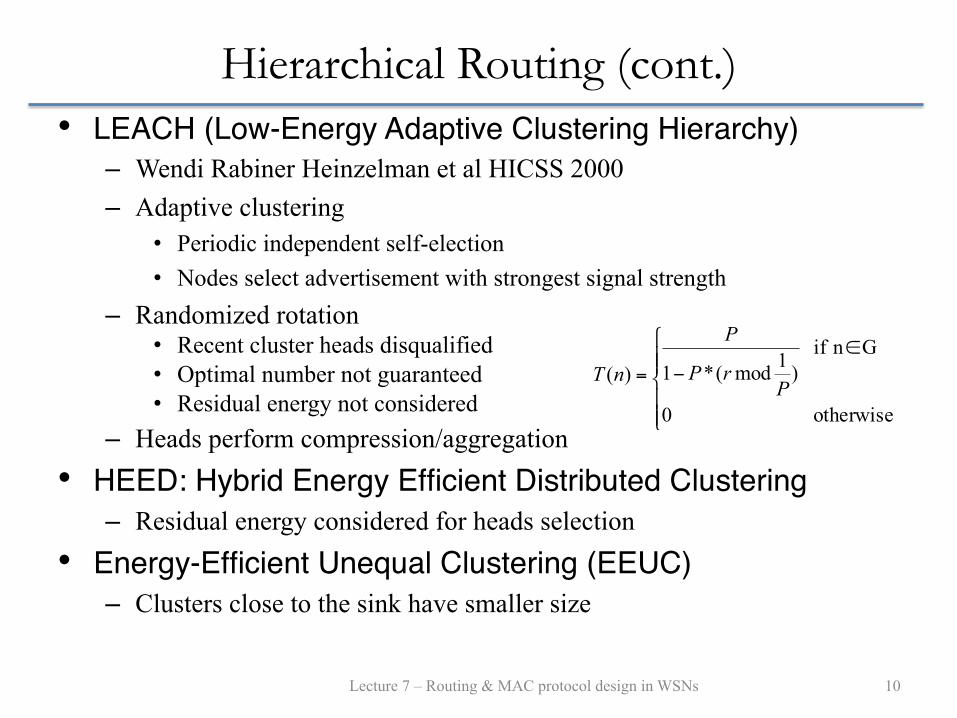
Hierarchical Routing (cont.) •  LEACH (Low-Energy Adaptive Clustering Hierarchy)

–  Wendi Rabiner Heinzelman et al HICSS 2000 –  Adaptive clustering

•  Periodic independent self-election •  Nodes select advertisement with strongest signal strength

–  Randomized rotation •  Recent cluster heads disqualified •  Optimal number not guaranteed •  Residual energy not considered

–  Heads perform compression/aggregation •  HEED: Hybrid Energy Efficient Distributed Clustering

–  Residual energy considered for heads selection •  Energy-Efficient Unequal Clustering (EEUC)

–  Clusters close to the sink have smaller size

⎪⎪⎩

⎪⎪⎨

⎧ ∈−=

otherwise 0

G n if )1mod(*1)(P

rP

P

nT


Geographic Routing


•  Key Idea – Make use of node location information in routing

•  Assumptions – Nodes know their own geographical location (e.g. GPS) – Nodes know their 1-hop neighbors – Routing destinations are specified geographically (a

location, or a geographical region) – Greedy localized routing

Geographic Routing (cont.)


•  GPSR: Greedy Perimeter Stateless Routing – Brad Karp and H. T. Kung (MobiCom 2000)

•  Greedy forwarding ing (GPSR). We aim for scalability under increasing numbers of

nodes in the network, and increasing mobility rate. As these fac-tors increase, our measures of scalability are:

Routing protocol message cost: How many routing protocolpackets does a routing algorithm send?

Application packet delivery success rate: What fraction ofapplications’ packets are delivered successfully by a routingalgorithm?

Per-node state: How much storage does a routing algorithmrequire at each node?

Networks that push on mobility, number of nodes, or both include:

Ad-hoc networks: Perhaps the most investigated category,these mobile networks have no fixed infrastructure, and sup-port applications for military users, post-disaster rescuers,and temporary collaborations among temporary associates,as at a business conference or lecture [10], [12], [20], [21],[22].

Sensor networks: Comprised of small sensors, these mobilenetworks can be deployed with very large numbers of nodes,and have very impoverished per-node resources [6], [13].Minimization of state per node in a network of tens of thou-sands of memory-poor sensors is crucial.

“Rooftop” networks: Proposed by Shepard [24], these wire-less networks are not mobile, but are deployed very denselyin metropolitan areas (the name refers to an antenna on eachbuilding’s roof, for line-of-sight with neighbors) as an alter-native to wired networking offered by traditional telecommu-nications providers. Such a network also provides an alter-nate infrastructure in the event of failure of the conventionalone, as after a disaster. A routing system that self-configures(without a trusted authority to configure a routing hierarchy)for hundreds of thousands of such nodes in a metropolitanarea represents a significant scaling challenge.

Traditional shortest-path (DV and LS) algorithms require state pro-portional to the number of reachable destinations at each router.On-demand ad-hoc routing algorithms require state at least pro-portional to the number of destinations a node forwards packetstoward, and often more, as in the case in DSR, in which a node ag-gressively caches all source routes it overhears to reduce the prop-agation scope of other nodes’ flooded route requests.

We will show that geographic routing allows routers to be nearlystateless, and requires propagation of topology information for onlya single hop: each node need only know its neighbors’ positions.The self-describing nature of position is the key to geography’susefulness in routing. The position of a packet’s destination andpositions of the candidate next hops are sufficient to make correctforwarding decisions, without any other topological information.

We assume in this work that all wireless routers know their ownpositions, either from a GPS device, if outdoors, or through othermeans. Practical solutions include surveying, for stationary wire-less routers; inertial sensors, on vehicles; and acoustic range-finding

y

x

D

Figure 1: Greedy forwarding example. y is x’s closest neighborto D.

using ultrasonic “chirps” indoors [28]. We further assume bidirec-tional radio reachability. The widely used IEEE 802.11 wirelessnetwork MAC [11] sends link-level acknowledgements for all uni-cast packets, so that all links in an 802.11 network must be bidi-rectional. We simulate a network that uses 802.11 radios to evalu-ate our routing protocol. We consider topologies where the wire-less nodes are roughly in a plane. Finally, we assume that packetsources can determine the locations of packet destinations, to markpackets they originate with their destination’s location. Thus, weassume a location registration and lookup service that maps nodeaddresses to locations [18]. Queries to this system use the samegeographic routing system as data packets; the querier geographi-cally addresses his request to a location server. The scope of thispaper is limited to geographic routing. We argue for the eminentpracticality of the location service briefly in Section 3.7. We adoptIP terminology throughout this paper, though GPSR can be appliedto any datagram network.

In the following sections, we describe the algorithms that compriseGPSR, measure and analyze GPSR’s performance and behaviorin simulated mobile networks, cite and differentiate related work,identify future research opportunities suggested by GPSR, and con-clude by summarizing our findings.

2. ALGORITHMS AND EXAMPLESWe now describe the Greedy Perimeter Stateless Routing algo-rithm. The algorithm consists of two methods for forwarding pack-ets: greedy forwarding, which is used wherever possible, and perime-ter forwarding, which is used in the regions greedy forwarding can-not be.

2.1 Greedy ForwardingAs alluded to in the introduction, under GPSR, packets are markedby their originator with their destinations’ locations. As a result,a forwarding node can make a locally optimal, greedy choice inchoosing a packet’s next hop. Specifically, if a node knows its ra-dio neighbors’ positions, the locally optimal choice of next hopis the neighbor geographically closest to the packet’s destination.Forwarding in this regime follows successively closer geographichops, until the destination is reached. An example of greedy next-hop choice appears in Figure 1. Here, x receives a packet destinedfor D. x’s radio range is denoted by the dotted circle about x, andthe arc with radius equal to the distance between y and D is shownas the dashed arc about D. x forwards the packet to y, as the dis-tance between y and D is less than that between D and any of x’sother neighbors. This greedy forwarding process repeats, until thepacket reaches D.

Geographic Routing (cont.)


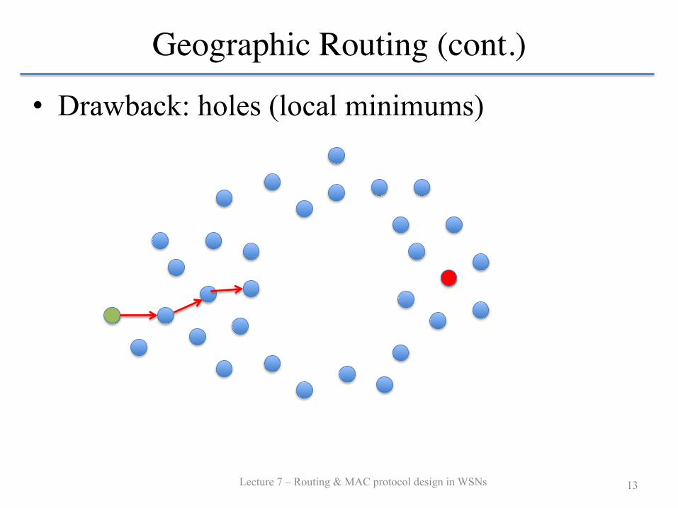
•  Drawback: holes (local minimums)

Graph Routing


•  LLNs: Low power and Lossy Networks – Devices have constraints in processing power, memory

and energy (battery power) –  Interconnection links have high loss rate, low data rate

and instability

•  RPL: IPv6 Routing Protocol for LLNs –  IETF draft – ROLL group - (Routing Over Low power and Lossy

networks) group

Graph Routing (cont.)


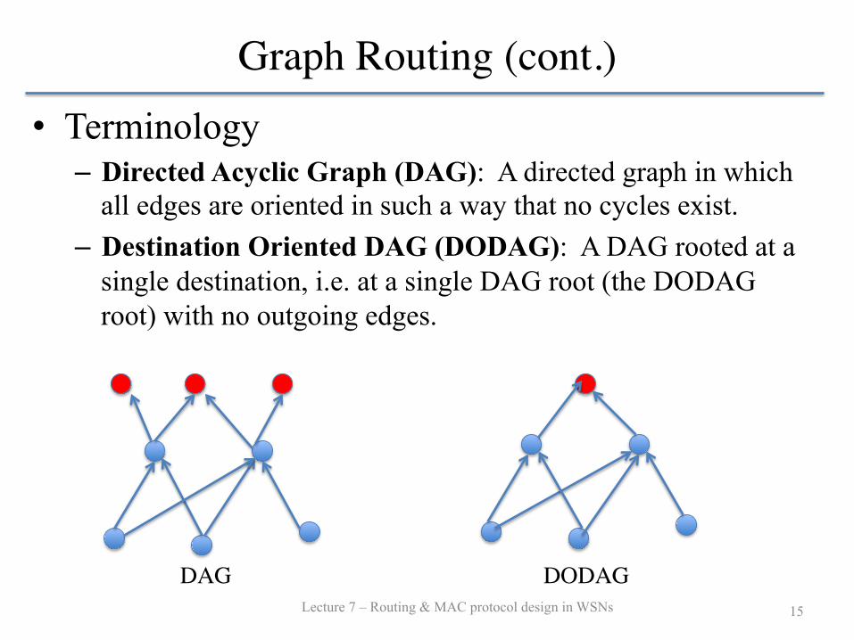
•  Terminology –  Directed Acyclic Graph (DAG): A directed graph in which

all edges are oriented in such a way that no cycles exist. –  Destination Oriented DAG (DODAG): A DAG rooted at a

single destination, i.e. at a single DAG root (the DODAG root) with no outgoing edges.

DAG DODAG

Architecture•  The communication architecture in Contiki


Application data, packet attributes

Collection protocol

Application 1 Application 2 Application 3

Routing protocol

Proprietary packet

format

MAC layer 2MAC layer 1 MAC layer 3

Application

data

Application

data

Rime stack

Chameleon

UDP/IP packets

802.15.4 frames

Figure 2. The Chameleon architecture. Applications andnetwork protocols run on top of the Rime stack. The out-put from Rime is transformed into different underlyingprotocols by header transformation modules.

3 The Chameleon ArchitectureThe Chameleon architecture is an adaptive communica-

tion architecture for sensor networks. The purpose of the ar-chitecture is threefold. First, the architecture is designed tosimplify the implementation of sensor network communica-tion protocols. This is done through the use of the Rime pro-tocol stack. Second, the architecture allows for sensor net-work protocols that are implemented on top of the architec-ture to take advantage of the features of underlying MAC andlink layer protocols. This is done by using packet attributesinstead of packet headers. Third, the architecture allows forthe packet headers of outgoing packets to be formed inde-pendently of the protocols or applications running within thearchitecture. Separate packet transformation modules handlepacket header construction.

The Chameleon architecture draws from previous workon sensor network architecture [10, 16, 30] and is inspiredby work in the area of distributed programming [20] andgeneral-purpose network architecture [3, 9].

Figure 2 shows the Chameleon architecture. The architec-ture contains three parts: the Rime stack, which provides aset of communication primitives to applications running ontop of the stack; a set of network protocols running on topof the Rime stack; and the Chameleon header transformationmodules, which create packets and packet headers from theoutput of the Rime stack. Applications run either directly ontop of the Rime stack, or on top of communication protocolsthat run on top of Rime.

The Chameleon header transformation modules can pro-duce either tightly bit-packed packet headers or headers thatconform either to specific MAC or link layer protocols, orto other communication protocols. Some header transforma-tion modules also implement parts of the protocol logic ofthe protocols they mimic.

Applications and protocols pass application data down tothe Rime stack. The Rime stack adds packet attributes tothe application data before it passes the application data andpacket attributes to the underlying Chameleon header trans-formation module. The header transformation module con-structs packet headers from the packet attributes and sendsthe final packets to the link-level device driver or the MAClayer. The MAC layer can inspect the packet attributes todecide how the packet should be transmitted. For example,broadcast packets may be sent differently from unicast pack-ets, and packets that need single-hop reliability can be sentwith link-layer acknowledgements turned on.

3.1 Separation of Protocol Logic and ProtocolHeaders

The protocol logic in the Rime stack does not deal withlow-level details of packet headers such as the placement,structure, and alignment of header fields. Rather, all man-agement of such low-level details is contained in the headertransformation modules.

Instead of using packet headers, the Chameleon archi-tecture uses packet attributes. Packet attributes contain thesame information that normally is found in packet headers.The packet attribute information is a more abstract represen-tation of the packet header information. Table 3.1 lists thepre-defined packet attributes in the Chameleon architecture.Both applications and lower layer protocols may define ad-ditional packet attributes.

The pre-defined packet attributes include the sender andreceiver addresses, packet IDs, packet types, the number oftimes that a packet has been forwarded, as well as feedbackinformation from the lower layers, such as the estimated linkquality, and information about radio congestion.

Each packet attribute has a scope. The scope of a packetattribute specifies how far the attribute will follow the packet.Attributes with scope 0 will only follow the packet within thenode, attributes with scope 1 will be transmitted in packetheaders but will not be forwarded across more than one node,and attributes with scope 2 will follow the packet to the finalrecipient in case of a multi-hop packet.

3.1.1 Header Field AlignmentThe headers in general purpose communication proto-

cols, such as the protocols in the TCP/IP stack, are typicallydefined so that all header fields are aligned on even byte-boundaries. The reason for this is that many microprocessorscannot access quantities that are not properly aligned.

Protocol designers must ensure that all header fieldsare properly aligned, and must therefore sometimes insertpadding bytes into the packet headers [24]. Low-power ra-dio protocols, however, must reduce their header size to aminimum and therefore in many cases cannot afford to alignall header fields.

With Chameleon’s packet attributes approach, the proto-col implementations do not have to deal with low-level align-ment of header fields. Rather, all low-level header alignmentdetails are contained in the header transformation modules.

3.1.2 Byte OrderingProtocols headers are typically designed to allow for hosts

with different byte order to communicate with each other.

•  A set of communication primitives

•  A set of network protocols

•  Tightly bit-packet packet headers

•  Headers that conform to specific MAC or link layer protocols.

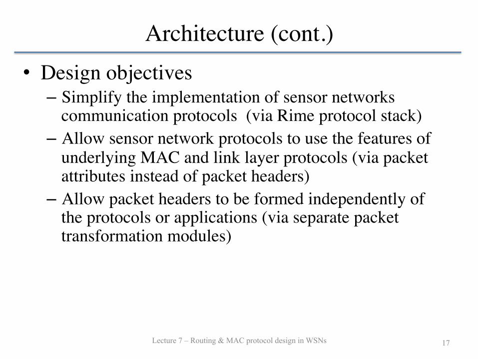
Architecture (cont.)•  Design objectives

–  Simplify the implementation of sensor networks communication protocols (via Rime protocol stack)

– Allow sensor network protocols to use the features of underlying MAC and link layer protocols (via packet attributes instead of packet headers)

– Allow packet headers to be formed independently of the protocols or applications (via separate packet transformation modules)


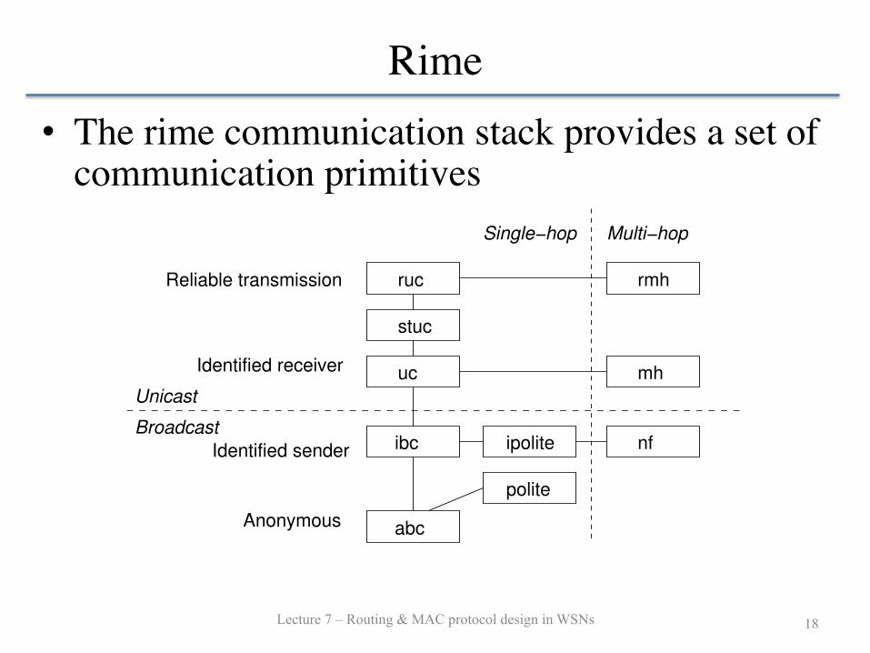
Rime•  The rime communication stack provides a set of

communication primitives


3.4 Lightweight LayeringThe Rime stack is built around a lightweight layering

principle. The communication primitives are designed in alayered fashion, where more complex communication prim-itives build on simpler ones. This is inspired by work in thearea of distributed programming [20], where many simplelayers are used to implement complex mechanisms such asnetwork consensus. The design with many simple layers al-lows for provable properties of composition of layers; weleave to future work to investigate if provable properties arepossible in the Rime stack.

For sensor networks, the lightweight layering principlehas several benefits. First, as the communication primitivesare simple, they are easy to implement and test. Second,the memory footprint of the implementations of the prim-itives is small, which is important for memory-constrainedsensor nodes. Third, as applications may attach to any layerof the stack, the applications can express precisely how muchof the communication features that they need. In moreheavyweight-layered stacks, such as the TCP/IP protocolstack, it generally is not possible to express such fine-grainedfeature requirements. For example, a TCP/IP application thatneeds congestion control but not guaranteed delivery cannotexpress this within the TCP/IP protocol architecture.

3.5 Header TransformationsThe header transformation modules in Chameleon pro-

duce headers from the packet attributes supplied by the Rimestack. Chameleon can transform the packet attributes into anarbitrary packet header format. By transforming the packetattributes into a standard packet format, the Chameleon ar-chitecture can become compatible with another node thatimplements the standard. However, header transformationsalone are not enough to mimic another communication pro-tocol.

3.6 Header Transformations Are Not EnoughThe header transformation mechanism is able to construct

headers that are compatible with any communication pro-tocol. However, a communication protocol is not definedby its protocol headers, but also by its protocol logic. Inmany cases, the Rime protocols already implement the pro-tocol logic required to fulfill the impersonated protocol. Inthose cases, the Chameleon header transformation moduleonly needs to create headers that match the impersonatedprotocol.

In case the protocol to be impersonated contains protocollogic not implemented by the Rime protocol, the Chameleonmodule must itself implement the missing parts of the proto-col logic of the protocols that it impersonates. For example, aUDP/IP header transformation module must implement theARP protocol if it is running over Ethernet, and a headertransformation module that translates a reliable bulk-transferRime protocol into a TCP stream must implement the SYN-ACK exchange before data transmission can start.

3.7 Feedback from Lower LayersThe protocols implemented in a header transformation

module may need to send feedback up to the application run-ning on top of Rime. Examples of this include both conges-tion notification and estimates of the radio link quality.

ruc rmh

stuc

uc mh

ibc ipolite nf

abc

polite

Identified sender

Anonymous

Reliable transmission

Identified receiver

Single−hop Multi−hop

Unicast

Broadcast

Figure 6. The communication primitives in the Rimestack and how they are layered.

Chameleon uses packet attributes to provide feedbackfrom the header transformation modules to the Rime stack.When an event occurs that needs be forwarded to the appli-cation, Chameleon associates the event with the channel onwhich the event occurred. The next time the channel is activeand a packet is sent towards the local application, Chameleonsets the appropriate packet attribute for the packet that is sentup through Rime. The feedback information may also bepiggybacked on acknowledgement packets that Chameleonproduces for the benefit of the application.

4 The Rime Protocol StackThe Rime protocol stack provides a set of communication

primitives, ranging from best-effort local neighbor broadcastand reliable local neighbor unicast, to best-effort networkflooding and hop-by-hop reliable multi-hop unicast. Appli-cations or protocols running on top of the Rime stack mayuse one or more of the communication primitives providedby the Rime stack.

4.1 Rime Communication PrimitivesThe protocols in the Rime stack are arranged in a layered

fashion, where the more complex protocols are implementedusing the less complex protocols. The communication prim-itives in the Rime stack and how they are arranged is shownin Figure 6.

We have chosen the communication primitives in theRime stack based on what typical sensor network protocolsuse. Applications or protocols running on top of the Rimestack attach at any layer of the stack and use any of the com-munication primitives.

The Rime stack supports both single-hop and multi-hopcommunication primitives. The multi-hop primitives do notspecify how packets are routed through the network. Instead,as the packet is sent across the network, the application orupper layer protocol is invoked at every node to choose thenext-hop neighbor. This makes it possible to implement ar-bitrary routing protocols on top of the multi-hop primitives.

4.1.1 Anonymous Best-effort Single-hop BroadcastThe anonymous best-effort single-hop broadcast prim-

itive (abc) is the most basic communication primitive inRime. The abc primitive provides a way for upper layersto send a data packet to all local neighbors that listen to the

Rime (cont.)•  Anonymous Best-effort Single-hop Broadcast (abc)

–  Send a data packet to all local neighbours that listen to the channel on which the packet is sent.

– No information about who sent the packet is included in the transmission.

– The most basic communication primitive. All other primitives are based on the abc primitive

•  Identified Best-effort Single-hop Broadcast (ibc)–  Same as abc but adds the single-hop sender address as a

packet attribute to the outgoing packets.


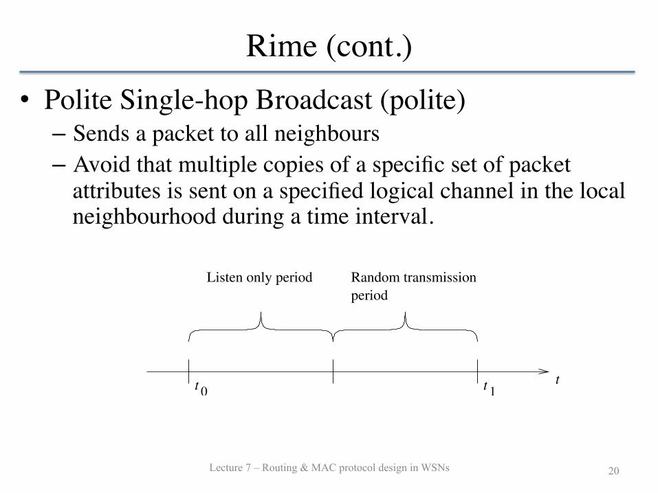
Rime (cont.)•  Polite Single-hop Broadcast (polite)

–  Sends a packet to all neighbours– Avoid that multiple copies of a specific set of packet

attributes is sent on a specified logical channel in the local neighbourhood during a time interval.


channel on which the packet is sent. No information aboutwho sent the packet is included in the transmission.

All other Rime primitives are based on the abc primitive.Normally, however, the abc primitive is not used directly byapplications or protocols that run on top of the Rime stack.When a packet is received by the abc module, the moduleimmediately passes the packet to the upper layer.

4.1.2 Identified Best-effort Single-hop BroadcastThe identified best-effort single-shop broadcast primitive

(ibc) sends a packet to all local neighbors. The ibc primitiveadds the single-hop sender address as a packet attribute tooutgoing packets. All Rime primitives that need the identityof the sender in the outgoing packets use the ibc primitive,either directly or indirectly through any of the other commu-nication primitives that are based on the ibc primitive.

4.1.3 Best-effort Single-hop UnicastThe best-effort single-hop unicast primitive (uc) sends a

packet to an identified single-hop neighbor. The uc primi-tive uses the ibc primitive and adds the single-hop receiveraddress attribute to the outgoing packets. For incomingpackets, the uc module inspects the single-hop receiver ad-dress attribute and discards the packet if the address does notmatch the address of the node.

4.1.4 Stubborn Single-hop UnicastThe stubborn single-hop unicast primitive (suc) repeat-

edly sends a packet to a single-hop neighbor using the ucprimitive. The stuc primitive sends and resends the packetuntil an upper layer primitive or protocol cancels the trans-mission. While it is possible for applications and protocolsthat use Rime to use the stubborn single-hop unicast primi-tive directly, the stuc primitive is primarily used by the reli-able single-hop unicast (ruc) primitive.

Before the stuc primitive sends a packet, it allocates aqueue buffer, to which the application data and packet at-tributes is copied, and sets a timer. When the timer expires,the stuc primitive copies the queue buffer to the Rime bufferand sends the packet using the uc primitive. The stuc prim-itive sets the number of retransmissions for a packet as apacket attribute on outgoing packets.

4.1.5 Reliable Single-hop UnicastThe reliable single-hop unicast primitive (ruc) reliably

sends a packet to a single-hop neighbor. The ruc primitiveuses acknowledgements and retransmissions to ensure thatthe neighbor successfully receives the packet. When the re-ceiver has acknowledged the packet, the ruc module notifiesthe sending application via a callback. The ruc primitive usesthe stubborn single-hop unicast primitive to do retransmis-sions. Thus, the ruc primitive does not have to manage thedetails of setting up timers and doing retransmissions, butcan concentrate on dealing with acknowledgements.

The ruc primitive adds two packet attributes: the single-hop packet type and the single-hop packet ID. The ruc prim-itive uses the packet ID attribute as a sequence number formatching acknowledgement packets to the correspondingdata packets.

The application or protocol that uses the ruc primitivecan specify the maximum number of transmissions that theruc module should attempt before the packet times out. If

Listen only period Random transmission

period

t 0 t 1t

Figure 7. Timeline of the algorithm used by the politebroadcast primitive.

a packet times out, the application or protocol that sent thepacket is notified with a callback.

4.1.6 Polite Single-hop BroadcastThe polite single-hop broadcast primitive (polite) is a gen-

eralization of the polite gossip algorithm from Trickle [25].The polite gossip algorithm is designed to reduce the totalamount of packet transmissions by not repeating a messagethat other nodes have already sent. The purpose of the po-lite broadcast primitive is to avoid that multiple copies of aspecific set of packet attributes is sent on a specified logicalchannel in the local neighborhood during a time interval.

The polite broadcast primitive is useful for implement-ing broadcast protocols that use, e.g., negative acknowledge-ments. If many nodes need to send the negative acknowl-edgement to a sender, it is enough if only a single message isdelivered to the sender.

The upper layer protocol or application that uses the po-lite broadcast primitive provides an interval time, and mes-sage along with a list of packet attributes for which multi-ple copies should be avoided. The polite broadcast primitivestores the outgoing message in a queue buffer, stores the listof packet attributes, and sets up a timer. The timer is set toa random time during the second half of the interval time, asshown in Figure 7.

During the first half of the time interval, the sender lis-tens for other transmissions. If it hears a packet that matchesthe attributes provided by the upper layer protocol or appli-cation, the sender drops the packet. The send timer has beenset to a random time some time during the second half ofthe interval. When the timer fires, and the sender has not yetheard a transmission of the same packet attributes, the senderbroadcasts its packet to all its neighbors.

The polite broadcast module does not add any packet at-tributes to outgoing packets apart from those added by theupper layer.

4.1.7 Identified Polite Single-hop BroadcastIdentified polite single-hop broadcasts (ipolite) works in

the same way as the polite primitive but adds the identity ofthe sender as a packet attribute through the use of the ibclayer.

4.1.8 Best-effort Multi-hop UnicastThe best-effort multi-hop unicast primitive (mh) sends a

packet to an identified node in the network by using multi-hop forwarding at each node in the network. The applica-tion or protocol that uses the mh primitive supplies a routingfunction for selecting the next-hop neighbor. If the mh prim-itive is requested to send a packet for which no suitable nexthop neighbor is found, the caller is immediately notified ofthis and may choose to initiate a route discovery process.

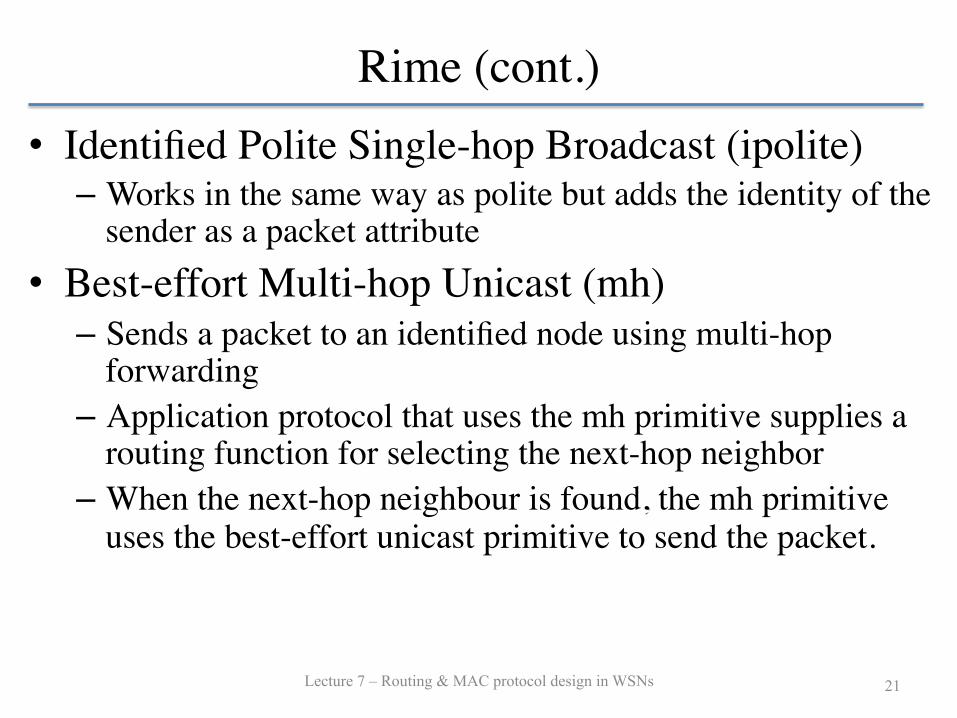
Rime (cont.)•  Identified Polite Single-hop Broadcast (ipolite)

– Works in the same way as polite but adds the identity of the sender as a packet attribute

•  Best-effort Multi-hop Unicast (mh)–  Sends a packet to an identified node using multi-hop

forwarding – Application protocol that uses the mh primitive supplies a

routing function for selecting the next-hop neighbor– When the next-hop neighbour is found, the mh primitive

uses the best-effort unicast primitive to send the packet.


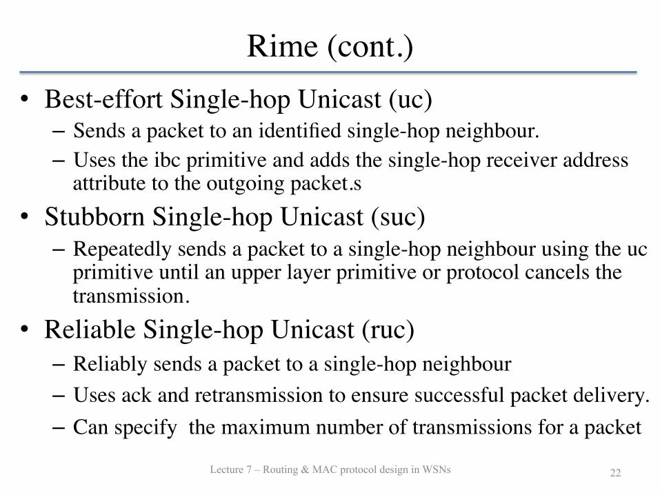
Rime (cont.)•  Best-effort Single-hop Unicast (uc)

–  Sends a packet to an identified single-hop neighbour.–  Uses the ibc primitive and adds the single-hop receiver address

attribute to the outgoing packet.s•  Stubborn Single-hop Unicast (suc)

–  Repeatedly sends a packet to a single-hop neighbour using the uc primitive until an upper layer primitive or protocol cancels the transmission.

•  Reliable Single-hop Unicast (ruc)–  Reliably sends a packet to a single-hop neighbour–  Uses ack and retransmission to ensure successful packet delivery. –  Can specify the maximum number of transmissions for a packet


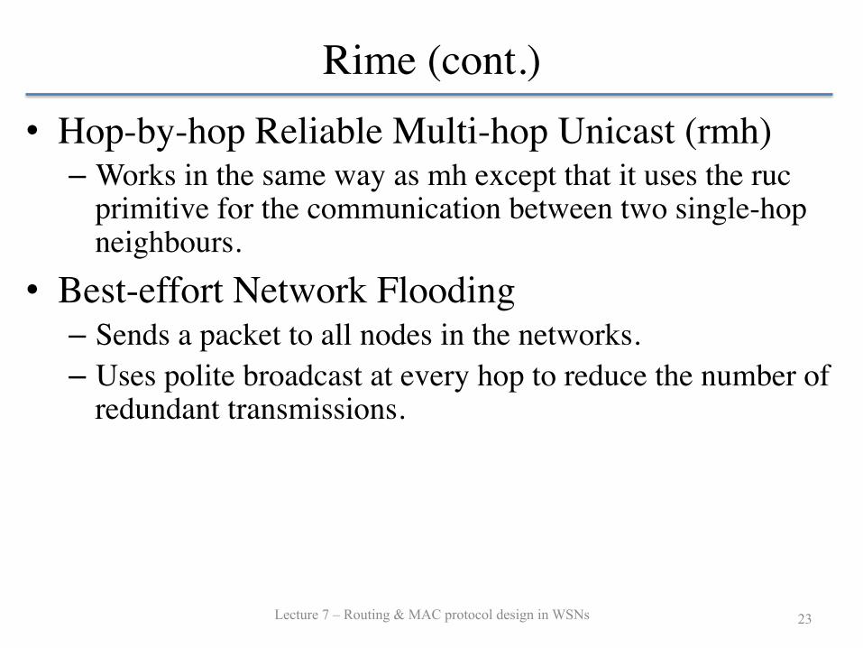
Rime (cont.)•  Hop-by-hop Reliable Multi-hop Unicast (rmh)

– Works in the same way as mh except that it uses the ruc primitive for the communication between two single-hop neighbours.

•  Best-effort Network Flooding–  Sends a packet to all nodes in the networks. – Uses polite broadcast at every hop to reduce the number of

redundant transmissions.


MAC Design Goals


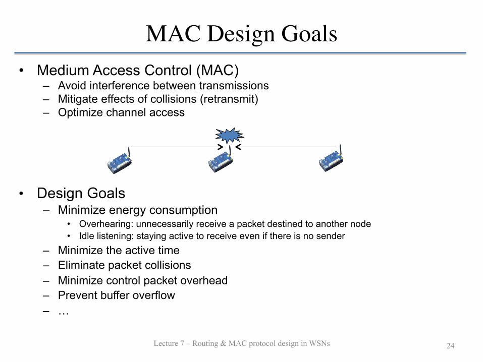
•  Medium Access Control (MAC) –  Avoid interference between transmissions –  Mitigate effects of collisions (retransmit) –  Optimize channel access

•  Design Goals –  Minimize energy consumption

•  Overhearing: unnecessarily receive a packet destined to another node •  Idle listening: staying active to receive even if there is no sender

–  Minimize the active time –  Eliminate packet collisions –  Minimize control packet overhead –  Prevent buffer overflow –  …

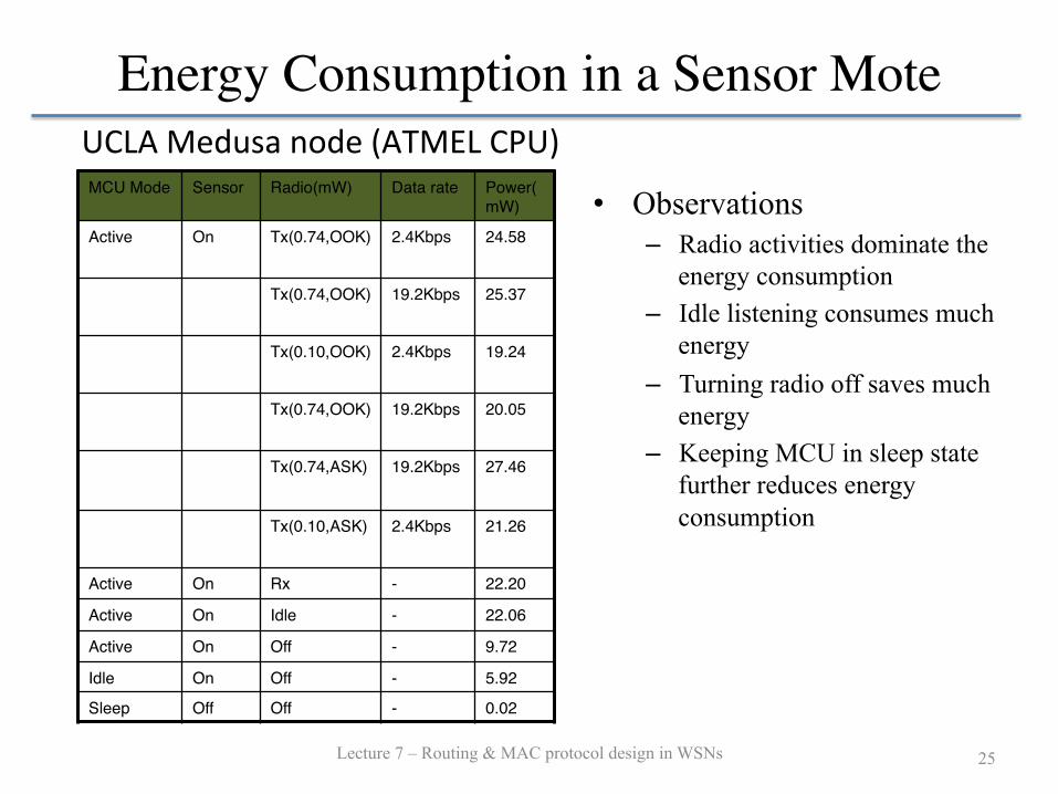
Energy Consumption in a Sensor Mote


•  Observations –  Radio activities dominate the

energy consumption –  Idle listening consumes much

energy –  Turning radio off saves much

energy –  Keeping MCU in sleep state

further reduces energy consumption

MCU Mode Sensor Radio(mW) Data rate Power(mW)

Active On Tx(0.74,OOK) 2.4Kbps 24.58

Tx(0.74,OOK) 19.2Kbps 25.37

Tx(0.10,OOK) 2.4Kbps 19.24

Tx(0.74,OOK) 19.2Kbps 20.05

Tx(0.74,ASK) 19.2Kbps 27.46

Tx(0.10,ASK) 2.4Kbps 21.26

Active On Rx - 22.20

Active On Idle - 22.06

Active On Off - 9.72

Idle On Off - 5.92

Sleep Off Off - 0.02

UCLA Medusa node (ATMEL CPU)

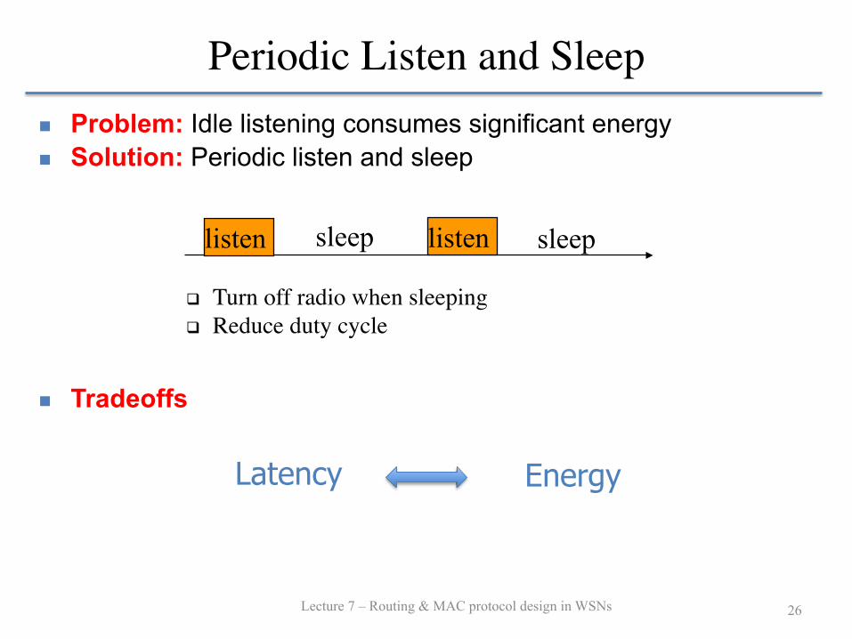
Periodic Listen and Sleep


n  Problem: Idle listening consumes significant energy n  Solution: Periodic listen and sleep

n  Tradeoffs

sleep listen listen sleep

Latency Energy

q  Turn off radio when sleepingq  Reduce duty cycle

S-MAC


•  S-MAC: An Energy-Efficient MAC Protocol for Wireless Sensor Networks –  Wei Ye, John Heidemann and Deborah Estrin, INFOCOM 2002

•  Key ideas: –  Idle listening --- Periodic listen and sleep–  Collision --- Using RTS and CTS–  Overhearing --- Interfering nodes go to sleep during transmission–  Control overhead --- Message passing

S-MAC (cont.)


•  Periodic listen and sleep –  Each node sleeps for some time, and then wakes up and listens to

see if any other node wants to talk to it –  All nodes are free to choose their own listen/sleep schedule, but

needs to synchronize with neighbors, that is, nodes and their neighbors listen at the same time and go sleep at the same time.

–  Synchronization is achieved by periodically broadcasting SYNC packets. 496 IEEE/ACM TRANSACTIONS ON NETWORKING, VOL. 12, NO. 3, JUNE 2004

Fig. 2. Neighboring nodes A and B have different schedules. Theysynchronize with nodes C and D respectively.

We call a complete cycle of listen and sleep a frame. The listeninterval is normally fixed according to physical-layer and MAC-layer parameters, e.g., the radio bandwidth and the contentionwindow size. The duty cycle is defined as the ratio of the listeninterval to the frame length. The sleep interval can be changedaccording to different application requirements, which actuallychanges the duty cycle. For simplicity, these values are the samefor all nodes.

All nodes are free to choose their own listen/sleep schedules.However, to reduce control overhead, we prefer neighboringnodes to synchronize together. That is, they listen at the sametime and go to sleep at the same time. It should be noticed thatnot all neighboring nodes can synchronize together in a mul-tihop network. Two neighboring nodes A and B may have dif-ferent schedules if they must synchronize with different nodes,C, and D, respectively, as shown in Fig. 2.

Nodes exchange their schedules by periodically broadcastinga SYNC packet to their immediate neighbors. A node talks to itsneighbors at their scheduled listen time, thus ensuring that allneighboring nodes can communicate even if they have differentschedules. In Fig. 2, for example, if node A wants to talk tonode B, it waits until B is listening. The period for a node tosend a SYNC packet is called the synchronization period.

One characteristic of S-MAC is that it forms nodes into aflat, peer-to-peer topology. Unlike clustering protocols, S-MACdoes not require coordination through cluster heads. Instead,nodes form virtual clusters around common schedules, but com-municate directly with peers. One advantage of this loose coor-dination is that it can be more robust to topology change thancluster-based approaches.

The downside of the scheme is the increased latency due tothe periodic sleeping. Furthermore, the delay can accumulate oneach hop. In Section IV, we will present a technique that is ableto significantly reduce such latency.

B. Collision Avoidance

If multiple neighbors want to talk to a node at the same time,they will try to send when the node starts listening. In this case,they need to contend for the medium. Among contention pro-tocols, the 802.11 does a very good job on collision avoidance.S-MAC follows similar procedures, including virtual and phys-ical carrier sense, and the RTS/CTS exchange for the hiddenterminal problem [14].

There is a duration field in each transmitted packet that in-dicates how long the remaining transmission will be. If a nodereceives a packet destined to another node, it knows how longto keep silent from this field. The node records this value in avariable called the network allocation vector (NAV) [1] and setsa timer for it. Every time when the timer fires, the node decre-ments its NAV until it reaches zero. Before initiating a trans-mission, a node first looks at its NAV. If its value is not zero, thenode determines that the medium is busy. This is called virtualcarrier sense.

Physical carrier sense is performed at the physical layer bylistening to the channel for possible transmissions. Carrier sensetime is randomized within a contention window to avoid colli-sions and starvations. The medium is determined as free if bothvirtual and physical carrier sense indicate that it is free.

All senders perform carrier sense before initiating a trans-mission. If a node fails to get the medium, it goes to sleepand wakes up when the receiver is free and listening again.Broadcast packets are sent without using RTS/CTS. Unicastpackets follow the sequence of RTS/CTS/DATA/ACK betweenthe sender and the receiver. After the successful exchange ofRTS and CTS, the two nodes will use their normal sleep time fordata packet transmission. They do not follow their sleep sched-ules until they finish the transmission.

With the low-duty-cycle operation and the contention mech-anism during each listen interval, S-MAC effectively addressesthe energy waste due to idle listening and collisions. In the nextsection, we will present details of the periodic sleep coordinatedamong neighboring nodes. Then we will present two techniquesthat further reduce the energy waste due to overhearing and con-trol overhead.

IV. COORDINATED SLEEPING

Periodic sleeping effectively reduces energy waste on idle lis-tening. In S-MAC, nodes coordinate their sleep schedules ratherthan randomly sleep on their own. This section details the pro-cedures that all nodes follow to set up and maintain their sched-ules. It also presents a technique to reduce latency due to theperiodic sleep on each node.

A. Choosing and Maintaining Schedules

Before each node starts its periodic listen and sleep, it needsto choose a schedule and exchange it with its neighbors. Eachnode maintains a schedule table that stores the schedules of allits known neighbors. It follows the steps below to choose itsschedule and establish its schedule table.

1) A node first listens for a fixed amount of time, which isat least the synchronization period. If it does not hear aschedule from another node, it immediately chooses itsown schedule and starts to follow it. Meanwhile, the nodetries to announce the schedule by broadcasting a SYNCpacket. Broadcasting a SYNC packet follows the normalcontention procedure. The randomized carrier sense timereduces the chance of collisions on SYNC packets.

2) If the node receives a schedule from a neighbor beforechoosing or announcing its own schedule, it follows thatschedule by setting its schedule to be the same. Then thenode will try to announce its schedule at its next sched-uled listen time.

3) There are two cases if a node receives a different scheduleafter it chooses and announces its own schedule. If thenode has no other neighbors, it will discard its currentschedule and follow the new one. If the node already fol-lows a schedule with one or more neighbors, it adoptsboth schedules by waking up at the listen intervals of thetwo schedules.

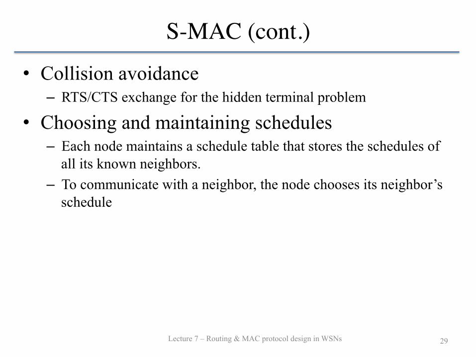
S-MAC (cont.)


•  Collision avoidance –  RTS/CTS exchange for the hidden terminal problem

•  Choosing and maintaining schedules –  Each node maintains a schedule table that stores the schedules of

all its known neighbors. –  To communicate with a neighbor, the node chooses its neighbor’s

schedule

S-MAC (cont.)


YE et al.: MAC WITH COORDINATED ADAPTIVE SLEEPING FOR WIRELESS SENSOR NETWORKS 497

To illustrate this algorithm, consider a network where allnodes can hear each other. The node who starts first will pickup a schedule first, and its broadcast will synchronize all itspeers on its schedule. If two or more nodes start first at thesame time, they will finish initial listening at the same time, andwill choose the same schedule independently. No matter whichnode sends out its SYNC packet first (wins the contention), itwill synchronize the rest of the nodes.

However, two nodes may independently assign schedules ifthey cannot hear each other in a multihop network. In this case,those nodes on the border of two schedules will adopt both. Forexample, nodes A and B in Fig. 2 will wake up at the listentime of both schedules. In this way, when a border node sends abroadcast packet, it only needs to send it once. The disadvantageis that these border nodes have less time to sleep and consumemore energy than others.

Another option is to let a border node adopt only oneschedule—the one it receives first. Since it knows that someother neighbors follow another schedule, it can still talk tothem. However, for broadcasting, it needs to send twice to thetwo different schedules. The advantage is that the border nodeshave the same simple pattern of periodic listen and sleep asother nodes.

We expect that nodes only rarely see multiple schedules, sinceeach node tries to follow an existing schedule before choosingan independent one. However, a new node may still fail to dis-cover an existing neighbor for a few reasons. The SYNC packetfrom the neighbor could be corrupted by collisions or interfer-ence. The neighbor may have delayed sending a SYNC packetdue to the busy medium. If the new node is on the border of twoschedules, it may only discover the first one if the two schedulesdo not overlap.

To prevent the case that two neighbors miss each other for-ever when they follow completely different schedules, S-MACintroduces periodic neighbor discovery, i.e., each node period-ically listens for the whole synchronization period. The fre-quency with which a node performs neighbor discovery dependson the number of neighbors it has. If a node does not haveany neighbor, it performs neighbor discovery more aggressivelythan in the case that it has many neighbors. Since the energycost is high during the neighbor discovery, it should not be per-formed too often. In our current implementation, the synchro-nization period is 10 s, and a node performs neighbor discoveryevery 2 min if it has at least one neighbor.

B. Maintaining Synchronization

Since neighboring nodes coordinate their sleep schedules,the clock drift on each node can cause synchronization errors.We use two techniques to make it robust to such errors. First,all exchanged timestamps are relative rather than absolute.Second, the listen period is significantly longer than clock driftrates. For example, the listen time of 0.5 s is more than 10times longer than typical clock drift rates. Compared to TDMAschemes with very short time slots, S-MAC requires muchlooser time synchronization.

Although the long listen time can tolerate fairly large clockdrift, neighboring nodes still need to periodically update each

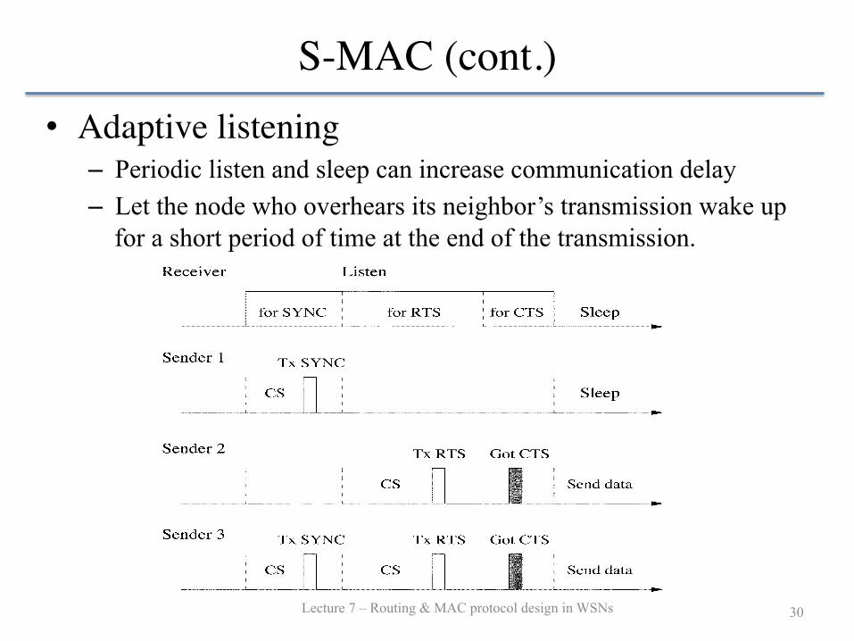
Fig. 3. Timing relationship between a receiver and different senders. CS standsfor carrier sense.

other with their schedules to prevent long-term clock drift. Thesynchronization period can be quite long. The measurements onour testbed nodes show that the clock drift between two nodesdoes not exceed 0.2 ms per second.

As mentioned earlier, schedule updating is accomplished bysending a SYNC packet. The SYNC packet is very short, andincludes the address of the sender and the time of its next sleep.The next sleep time is relative to the moment that the senderstarts transmitting the SYNC packet. When a receiver gets thetime from the SYNC packet it subtracts the packet transmissiontime and use the new value to adjust its timer.

In order for a node to receive both SYNC packets and datapackets, we divide its listen interval into two parts. The first oneis for SYNC packets, and the second one is for data packets, asshown in Fig. 3. Each part has a contention window with manytime slots for senders to perform carrier sense. For example, if asender wants to send a SYNC packet, it starts carrier sense whenthe receiver begins listening. It randomly selects a time slot tofinish its carrier sense. If it has not detected any transmission bythe end of that time slot, it wins the contention and starts sendingits SYNC packet. The same procedure is followed when sendingdata packets.

Fig. 3 shows the timing relationship of three possible situa-tions that a sender transmits to a receiver. Sender 1 only sendsa SYNC packet. Sender 2 only sends a unicast data packet.Sender 3 sends both a SYNC and a data packet.

C. Adaptive Listening

The scheme of periodic listen and sleep is able to signifi-cantly reduce the time spent on idle listening when traffic loadis light. However, when a sensing event indeed happens, it isdesirable that the sensing data can be passed through the net-work without too much delay. When each node strictly followsits sleep schedule, there is a potential delay on each hop, whoseaverage value is proportional to the length of the frame. Wetherefore introduce a mechanism to switch the nodes from thelow-duty-cycle mode to a more active mode in this case.

•  Adaptive listening–  Periodic listen and sleep can increase communication delay –  Let the node who overhears its neighbor’s transmission wake up

for a short period of time at the end of the transmission.

T-MAC


•  T-MAC: An Adaptive Energy-Efficient MAC Protocol for Wireless Sensor Networks –  Tijs van Dam and Koen Langendoen, SenSys 2003

•  Key ideas: –  Reduce idle listening by transmitting all messages in bursts

of variable length, and sleeping between bursts. –  Dynamically determine the optimal length of active time

based on the traffic load.

T-MAC (cont.)


•  Overview

–  RTS/CTS/ACK –  An active period ends when none of the following events

has occurred during a period of TA •  The firing of a periodic frame timer •  Receiving data packets •  Sense radio activity •  The end-of-transmission of a node’s own packet or acknowledgement •  The knowledge that a data exchange of a neighbor has ended.

active state

sleep state

normal

S-MAC

Figure 1: The S-MAC duty cycle; the arrowsindicate transmitted and received messages; notethat messages come closer together.

can communicate with its neighbors and send any messagesqueued during the sleeping part, as shown in Figure 1. Sinceall messages are packed into the active part, instead of be-ing ‘spread out’ over the whole frame, the time betweenmessages, and therefore the energy wasted on idle listening,is reduced.

S-MAC needs some synchronization, but that is not ascritical as in TDMA-based protocols: the time scale is muchlarger. Typically, there may be an active part of 200 ms ina frame of one second. A clock drift of 500 µs will not be aproblem.

The S-MAC protocol essentially trades used energy forthroughput and latency. Throughput is reduced becauseonly the active part of the frame is used for communication.Latency increases because a message-generating event mayoccur during sleep time. In that case, the message will bequeued until the start of the next active part.

3. T-MAC PROTOCOL DESIGNEnergy consumption is the main criterion for our MAC

protocol design. We have already identified the problem ofidle listening. Other forms of energy waste are:

collisions if two nodes transmit at the same time and in-terfere with each others transmission, packets are cor-rupted. Hence, the energy used during transmissionand reception is wasted;

protocol overhead most protocols require control packetsto be exchanged; as these contain no application data,we may consider any energy used for transmitting andreceiving these packets as overhead;

overhearing since the air is a shared medium, a node mayreceive packets that are not destined for it; it couldthen as well have turned off its radio.

These other sources of energy consumption are relativelyinsignificant when compared to the energy wasted by idlelistening, especially when messages are infrequent. Considerour example where 99% of the time is spent on idle listen-ing. If, then, the actual transmission and receiving timeincreases by a factor two—due to collisions and overhead—,idle listening time decreases only from 99% to 98%.

Although reducing the idle listening time, a solution with afixed duty cycle, like the S-MAC protocol [12], is not optimal.S-MAC has two important parameters: the total frame time,which is limited by latency requirements and buffer space,and the active time. The active time depends mainly onthe message rate: it can be so small that nodes are able totransfer all their messages within the active time.

active time

sleep time

normal

T-MACTA TA TA

Figure 2: The basic T-MAC protocol scheme, withadaptive active times.

The problem is that, while latency requirements and bufferspace are generally fixed, the message rate will usually vary(Section 1.1). If important messages are not to be missed–and unimportant messages should not have been sent in anycase–, the nodes must be deployed with an active time thatcan handle the highest expected load. Whenever the load islower than that, the active time is not optimally used andenergy will be wasted on idle listening.

The novel idea of the T-MAC protocol is to reduce idlelistening by transmitting all messages in bursts of variablelength, and sleeping between bursts. To maintain an optimalactive time under variable load, we dynamically determineits length. We end the active time in an intuitive way: wesimply time out on hearing nothing.

3.1 Basic protocolFigure 2 shows the basic scheme of the T-MAC protocol.

Every node periodically wakes up to communicate with itsneighbors, and then goes to sleep again until the next frame.Meanwhile, new messages are queued. Nodes communi-cate with each other using a Request-To-Send (RTS), Clear-To-Send (CTS), Data, Acknowledgement (ACK) scheme,which provides both collision avoidance and reliable trans-mission [1]. This scheme is well known and used, for exam-ple, in the IEEE 802.11 standard [4].

A node will keep listening and potentially transmitting,as long as it is in an active period. An active period endswhen no activation event has occurred for a time TA. Anactivation event is:

• the firing of a periodic frame timer;

• the reception of any data on the radio;

• the sensing of communication1 on the radio, e.g. dur-ing a collision;

• the end-of-transmission of a node’s own data packet oracknowledgement;

• the knowledge, through overhearing prior RTS andCTS packets, that a data exchange of a neighbor hasended.

A node will sleep if it is not in an active period. Conse-quently, TA determines the minimal amount of idle listeningper frame.

The described timeout scheme moves all communicationto a burst at the beginning of the frame. Since messagesbetween active times must be buffered, the buffer capacitydetermines an upper bound on the maximum frame time.1Through a Received Signal Strength Indication (RSSI)signal from the radio.

173

B-MAC


•  B-MAC: Berkeley Media Access Control for low power wireless sensor networks –  “Versatile Low Power Media Access for Wireless Sensor

Networks”, Joseph Polastre, Jason Hill, and David Culler, SenSys 2004

•  Key ideas: –  Low power listening (LPL) for low power communication. –  Clear channel assessment (CCA) and packet backoff for

channel arbitration –  Link layer acknowledge for reliability

B-MAC (cont.)


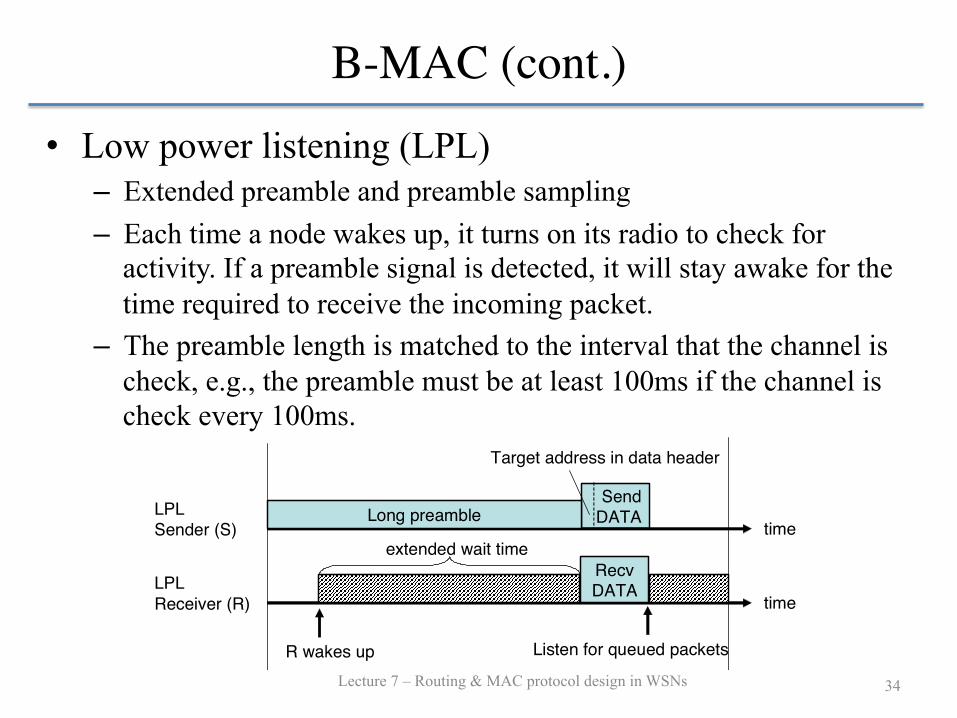
•  Low power listening (LPL) –  Extended preamble and preamble sampling –  Each time a node wakes up, it turns on its radio to check for

activity. If a preamble signal is detected, it will stay awake for the time required to receive the incoming packet.

–  The preamble length is matched to the interval that the channel is check, e.g., the preamble must be at least 100ms if the channel is check every 100ms.

SendDATA time

Long preambleLPLSender (S)

Target address in data header

timeLPLReceiver (R)

R wakes up

timeX-MACSender (S)

SendDATA

timeX-MACReceiver (R)

RecvDATA

R wakes up

Short preambles withtarget address information

ACK

Receive early ACK

Send early ACK

extended wait time

Time & energysaved at S & R

RecvDATA

Listen for queued packets

Figure 1. Comparison of the timelines between LPL’sextended preamble and X-MAC’s short preamble ap-proach.

hearing, excessive preamble and incompatibility with pack-etizing radios.3.1 Asynchronous Duty CyclingA visual representation of asynchronous low power lis-

tening (LPL) duty cycling is shown in the top section ofFigure 1. When a node has data to send, it first transmitsan extended preamble, and then sends the data packet. Allother nodes maintain their own unsynchronized sleep sched-ules. When the receiver awakens, it samples the medium. Ifa preamble is detected, the receiver remains awake for theremainder of the long preamble, then determines if it is thetarget. After receiving the full preamble, if the receiver is notthe target, it goes back to sleep.3.2 Embedding the Target ID in the Preamble

to Avoid OverhearingA key limitation of LPL is that non-target receivers who

wake and sample the medium while a preamble is being sentmust wait until the end of the extended preamble before find-ing out that they are not the target and should go back tosleep. This is termed as the overhearing problem, and ac-counts for much of the inefficiency and wasted energy incurrent asynchronous techniques. This means that for ev-ery transmission, the energy expended is proportional to thenumber of receivers in range. Hence, the energy usage isdependent on density as well as traffic load. This problemis exacerbated by the fact that sensor networks are often de-ployed with high node densities in order to provide sensingat a fine granularity.In X-MAC, we ameliorate the overhearing problem by di-

viding the one long preamble into a series of short preamblepackets, each containing the ID of the target node, as indi-cated in Figure 1. The stream of short preamble packets ef-fectively constitutes a single long preamble. When a nodewakes up and receives a short preamble packet, it looks atthe target node ID that is included in the packet. If the nodeis not the intended recipient, the node returns to sleep imme-diately and continues its duty cycling as if the medium had

been idle. If the node is the intended recipient, it remainsawake for the subsequent data packet. As seen in the figure,a node can quickly return to sleep, thus avoiding the over-hearing problem.With this technique, the energy expenditure is signifi-

cantly less affected by network density. The approach of aseries of short preamble packets scales well with increasingdensity, i.e. as the number of senders increases in a neigh-borhood, energy expenditure remains largely flat. In com-parison, as the number of senders increase in each neighbor-hood of a WSN using LPL, the entire WSN stays awake forincreasing amounts of time.Another advantage of this approach is that it can be em-

ployed on all types of radios. Any packetizing radio, suchas the CC2420 characteristic of MICAz and TelosB motes,the CC2500, and/or the XBee, will be capable of sending aseries of short packets containing the target ID. As we willsee later, such universal support across packetizing radios isnot true of the traditional extended preamble LPL. In addi-tion, the short preamble packets can be supported across allradios with bit streaming interfaces, e.g. the CC1000 that isfound in the MICA2 mote.

3.3 Reducing Excessive Preamble usingStrobing

Using an extended preamble and preamble sampling al-lows for low power communications, yet even greater en-ergy savings are possible if the total time spent transmit-ting preambles is reduced. In traditional asynchronous tech-niques, the sender sends the entire preamble even though,on average, the receiver will wake up half way through thepreamble. The entire preamble needs to be sent before everydata transmission because there is no way for the sender toknow that the receiver has woken up. This is one case wheremore time is spent sending the preamble than is necessary,as illustrated by the extended wait time in Figure 1. Anothercase occurs when there are a number of transmitters waitingto send to a particular receiver. After the first sender beginstransmitting preamble packets, subsequent transmitters willstay awake and wait until the channel is clear. They willthen begin sending their preamble, and this occurs for everysubsequent sender. Consequently, each sender transmits theentire preamble when in fact the receiver was woken up bythe first transmitter in the series.In the development of X-MAC, we provide solutions for

both of these cases. Instead of sending a constant stream ofpreamble packets, as would most closely approximate tradi-tional LPL, we insert small pauses between packets the seriesof short preamble packets, during which time the transmit-ting node pauses to listen to the medium. These gaps enablethe receiver to send an early acknowledgment packet backto the sender by transmitting the acknowledgment duringthe short pause between preamble packets. When a senderreceives an acknowledgment from the intended receiver, itstops sending preambles and sends the data packet. This al-lows the receiver to cut short the excessive preamble, whichreduces per-hop latency and energy spent unnecessarily wait-ing and transmitting, as can be seen in Figure 1. Since thesender quickly alternates between a short preamble packet

B-MAC (cont.)


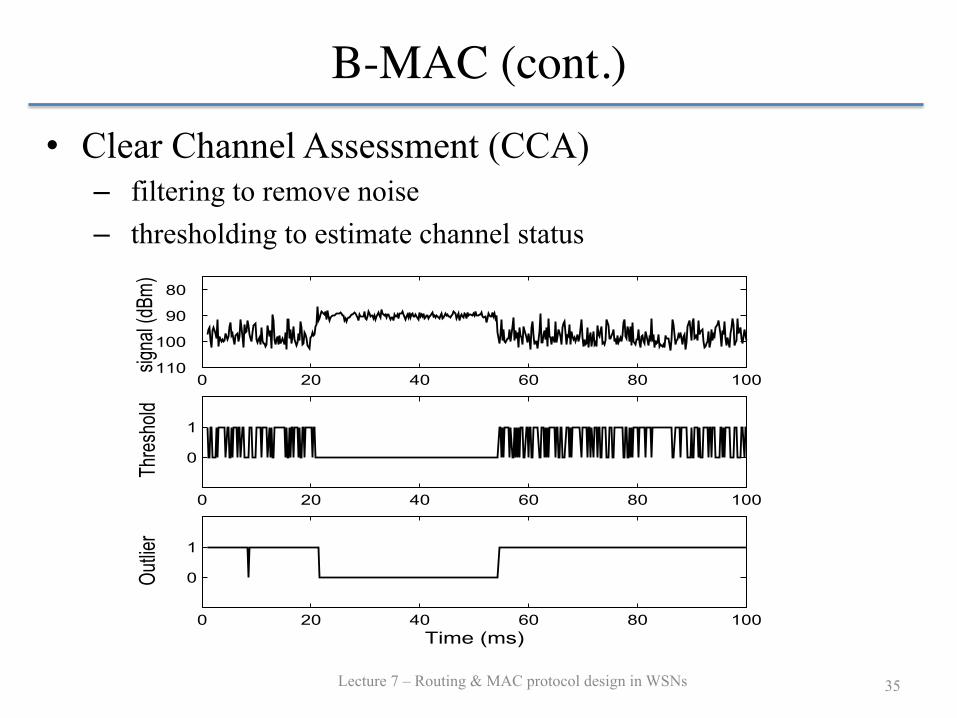
•  Clear Channel Assessment (CCA) –  filtering to remove noise –  thresholding to estimate channel status

interface MacControl {command result_t EnableCCA();command result_t DisableCCA();command result_t EnableAck();command result_t DisableAck();command void* HaltTx();

}

interface MacBackoff {event uint16_t initialBackoff(void* msg);event uint16_t congestionBackoff(void* msg);

}

interface LowPowerListening {command result_t SetListeningMode(uint8_t mode);command uint8_t GetListeningMode();command result_t SetTransmitMode(uint8_t mode);command uint8_t GetTransmitMode();command result_t SetPreambleLength(uint16_t bytes);command uint16_t GetPreambleLength();command result_t SetCheckInterval(uint16_t ms);command uint16_t GetCheckInterval();

}

Figure 1: Interfaces for flexible control of B-MAC by higherlayer services. These TinyOS interfaces allow services to tog-gle CCA and acknowledgments, set backoffs on a per messagebasis, and change the LPL mode for transmit and receive.

through repeated rounds of resynchronization.T-MAC [19] improves on S-MAC’s energy usage by using a very

short listening window at the beginning of each active period. Afterthe SYNC section of the active period, there is a short window tosend or receive RTS and CTS packets. If no activity occurs in thatperiod, the node returns to sleep. By changing the protocol to havean adaptive duty cycle, T-MAC saves power at a cost of reducedthroughput and additional latency. T-MAC, in variable workloads,uses one fifth the power of S-MAC. In homogeneous workloads, T-MAC and S-MAC perform equally well. T-MAC suffers from thesame complexity and scaling problems of S-MAC. Shortening theactive window in T-MAC reduces the ability to snoop on surround-ing traffic and adapt to changing network conditions.Many of these protocols have only been evaluated in simulation.

Not only must the protocol perform well in simulation, it must alsointegrate well with the implementation of wireless sensor networkapplications. Each of the protocols described in this section providesolutions that meet a subset of our goals. Motivated by monitoringapplications for wireless sensor networks, we build upon ideas frompreviously published work to create a reconfigurable protocol thatmeets all of the goals from Section 1.

3. DESIGN AND IMPLEMENTATIONTo achieve the goals outlined in Section 1, we designed a CSMA

protocol for wireless sensor networks called B-MAC, BerkeleyMe-dia Access Control for low power wireless sensor networks. Al-though B-MAC is motivated by the needs of monitoring applica-tions, the flexibility of our protocol allows allows other servicesand applications to be realized efficiently. These services include,but are not limited to, target tracking, localization, triggered eventreporting, and multihop routing.Classical MAC protocols perform channel access arbitration and

are tuned for good performance over a set of workloads thoughtto be representative of the domain. S-MAC is an example of awireless sensor network protocol designed using a classical ap-proach. S-MAC provides an RTS-CTS mechanism for channel ar-

0 20 40 60 80 100110

100

90

80

signa

l (dBm

)

0 20 40 60 80 100

0

1

Thre

shold

0 20 40 60 80 100

0

1

Time (ms)

Outlie

r

Figure 2: Clear Channel Assessment (CCA) effectiveness for atypical wireless channel. The top graph is a trace of the receivedsignal strength indicator (RSSI) from a CC1000 transceiver. Apacket arrives between 22 and 54ms. The middle graph showsthe output of a thresholding CCA algorithm. 1 indicates thechannel is clear, 0 indicates it is busy. The bottom graph showsthe output of an outlier detection algorithm.

bitration and hidden terminal avoidance, synchronization with itsneighbors for low power operation, and message fragmentation forefficiently transferring bulk data. S-MAC is not only a link proto-col, but also network and organization protocol. Applications andservices must rely on S-MAC’s internal policies to adjust its op-eration as node and network conditions change; such changes areopaque to the application. In contrast, the B-MAC protocol con-tains a small core of media access functionality. B-MAC uses clearchannel assessment (CCA) and packet backoffs for channel arbitra-tion, link layer acknowledgments for reliability, and low power lis-tening (LPL) for low power communication. B-MAC is only a linkprotocol, with network services like organization, synchronization,and routing built above its implementation. Although B-MAC nei-ther provides multi-packet mechanisms like hidden terminal sup-port or message fragmentation nor enforces a particular low powerpolicy, B-MAC has a set of interfaces that allow services to tune itsoperation (shown in Figure 1) in addition to the standard messageinterfaces1. These interfaces allow network services to adjust B-MAC’s mechanisms, including CCA, acknowledgments, backoffs,and LPL. By exposing a set of configurable mechanisms, protocolsbuilt on B-MAC make local policy decisions to optimize powerconsumption, latency, throughput, fairness or reliability.For effective collision avoidance, a MAC protocol must be able

to accurately determine if the channel is clear, referred to as ClearChannel Assessment (CCA). Since the ambient noise changes de-pending on the environment, B-MAC employs software automaticgain control for estimating the noise floor. Signal strength samplesare taken at times when the channel is assumed to be free–such asimmediately after transmitting a packet or when the data path ofthe radio stack is not receiving valid data. Samples are then en-tered into a FIFO queue. The median of the queue is added to anexponentially weighted moving average with decay �. The median1Standard interfaces for message transmission in TinyOS [18] areBareSendMsg for transmission, ReceiveMsg for reception,and RadioCoordinator for time stamping and start of framedelimiter (SFD) information.

97

X-MAC


•  X-MAC: A Short Preamble MAC Protocol for Duty-Cycled Wireless Sensor Networks –  Michael Buettner, Gary V. Yee, Eric Anderson and Richard

Han, SenSys 2006

•  Key ideas: –  employs a short preamble to further reduce energy

consumption and to reduce latency. –  embed address information of the target in the preamble so

that non-target receivers can quickly go back to sleep –  use a strobed preamble to allow the target receiver to

interrupt the long preamble as soon as it wakes up and determines that it is the target receiver.

X-MAC (cont.)


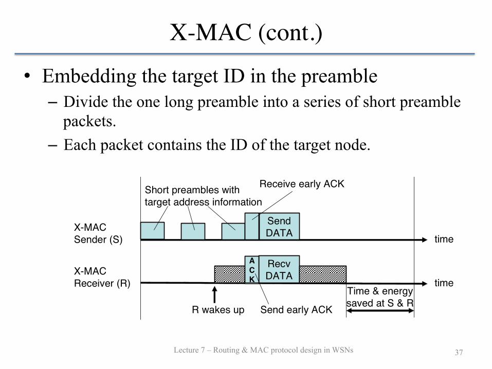
•  Embedding the target ID in the preamble –  Divide the one long preamble into a series of short preamble

packets. –  Each packet contains the ID of the target node.

SendDATA time

Long preambleLPLSender (S)

Target address in data header

timeLPLReceiver (R)

R wakes up

timeX-MACSender (S)

SendDATA

timeX-MACReceiver (R)

RecvDATA

R wakes up

Short preambles withtarget address information

ACK

Receive early ACK

Send early ACK

extended wait time

Time & energysaved at S & R

RecvDATA

Listen for queued packets

Figure 1. Comparison of the timelines between LPL’sextended preamble and X-MAC’s short preamble ap-proach.

hearing, excessive preamble and incompatibility with pack-etizing radios.3.1 Asynchronous Duty CyclingA visual representation of asynchronous low power lis-

tening (LPL) duty cycling is shown in the top section ofFigure 1. When a node has data to send, it first transmitsan extended preamble, and then sends the data packet. Allother nodes maintain their own unsynchronized sleep sched-ules. When the receiver awakens, it samples the medium. Ifa preamble is detected, the receiver remains awake for theremainder of the long preamble, then determines if it is thetarget. After receiving the full preamble, if the receiver is notthe target, it goes back to sleep.3.2 Embedding the Target ID in the Preamble

to Avoid OverhearingA key limitation of LPL is that non-target receivers who

wake and sample the medium while a preamble is being sentmust wait until the end of the extended preamble before find-ing out that they are not the target and should go back tosleep. This is termed as the overhearing problem, and ac-counts for much of the inefficiency and wasted energy incurrent asynchronous techniques. This means that for ev-ery transmission, the energy expended is proportional to thenumber of receivers in range. Hence, the energy usage isdependent on density as well as traffic load. This problemis exacerbated by the fact that sensor networks are often de-ployed with high node densities in order to provide sensingat a fine granularity.In X-MAC, we ameliorate the overhearing problem by di-

viding the one long preamble into a series of short preamblepackets, each containing the ID of the target node, as indi-cated in Figure 1. The stream of short preamble packets ef-fectively constitutes a single long preamble. When a nodewakes up and receives a short preamble packet, it looks atthe target node ID that is included in the packet. If the nodeis not the intended recipient, the node returns to sleep imme-diately and continues its duty cycling as if the medium had

been idle. If the node is the intended recipient, it remainsawake for the subsequent data packet. As seen in the figure,a node can quickly return to sleep, thus avoiding the over-hearing problem.With this technique, the energy expenditure is signifi-

cantly less affected by network density. The approach of aseries of short preamble packets scales well with increasingdensity, i.e. as the number of senders increases in a neigh-borhood, energy expenditure remains largely flat. In com-parison, as the number of senders increase in each neighbor-hood of a WSN using LPL, the entire WSN stays awake forincreasing amounts of time.Another advantage of this approach is that it can be em-

ployed on all types of radios. Any packetizing radio, suchas the CC2420 characteristic of MICAz and TelosB motes,the CC2500, and/or the XBee, will be capable of sending aseries of short packets containing the target ID. As we willsee later, such universal support across packetizing radios isnot true of the traditional extended preamble LPL. In addi-tion, the short preamble packets can be supported across allradios with bit streaming interfaces, e.g. the CC1000 that isfound in the MICA2 mote.

3.3 Reducing Excessive Preamble usingStrobing

Using an extended preamble and preamble sampling al-lows for low power communications, yet even greater en-ergy savings are possible if the total time spent transmit-ting preambles is reduced. In traditional asynchronous tech-niques, the sender sends the entire preamble even though,on average, the receiver will wake up half way through thepreamble. The entire preamble needs to be sent before everydata transmission because there is no way for the sender toknow that the receiver has woken up. This is one case wheremore time is spent sending the preamble than is necessary,as illustrated by the extended wait time in Figure 1. Anothercase occurs when there are a number of transmitters waitingto send to a particular receiver. After the first sender beginstransmitting preamble packets, subsequent transmitters willstay awake and wait until the channel is clear. They willthen begin sending their preamble, and this occurs for everysubsequent sender. Consequently, each sender transmits theentire preamble when in fact the receiver was woken up bythe first transmitter in the series.In the development of X-MAC, we provide solutions for

both of these cases. Instead of sending a constant stream ofpreamble packets, as would most closely approximate tradi-tional LPL, we insert small pauses between packets the seriesof short preamble packets, during which time the transmit-ting node pauses to listen to the medium. These gaps enablethe receiver to send an early acknowledgment packet backto the sender by transmitting the acknowledgment duringthe short pause between preamble packets. When a senderreceives an acknowledgment from the intended receiver, itstops sending preambles and sends the data packet. This al-lows the receiver to cut short the excessive preamble, whichreduces per-hop latency and energy spent unnecessarily wait-ing and transmitting, as can be seen in Figure 1. Since thesender quickly alternates between a short preamble packet

X-MAC (cont.)


•  Reducing excessive preamble using strobing –  Insert small gaps between the series of short preamble

packets. –  These gaps enable the receiver to send an early

acknowledgement during the short pause between preamble packets.

–  When a sender receives an acknowledgement for the intended receiver, it stops sending the preamble and starts sending the data packet

RI-MAC


•  RI-MAC: A Receiver-Initiated Asynchronous Duty Cycle MAC Protocol for Dynamic Traffic Loads in Wireless Sensor Networks –  Yanjun Sun, Omer Gurewitz, and David B. Johnson, SenSys

2008

•  Key Idea –  Receiver-Initiated, which uses receiver-initiated data

transmission in order to efficiently and effectively operate over a wide range of traffic loads.

RI-MAC (cont.)


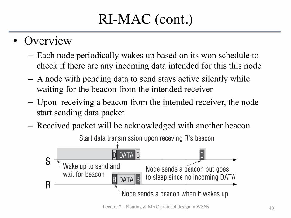
•  Overview –  Each node periodically wakes up based on its won schedule to

check if there are any incoming data intended for this this node –  A node with pending data to send stays active silently while

waiting for the beacon from the intended receiver –  Upon receiving a beacon from the intended receiver, the node

start sending data packet –  Received packet will be acknowledged with another beacon

BDATA

DATA

B

B B

B

R

S

Node sends a beacon when it wakes up

Wake up to send and wait for beacon

Start data transmission upon receving R’s beacon

Node sends a beacon but goesto sleep since no incoming DATA

Figure 3: Overview of RI-MAC. Each node periodically wakesup and broadcasts a beacon. When node S wants to send aDATA frame to node R, it stays active silently and starts DATAtransmission upon receiving a beacon from R. Node S laterwakes up but goes to sleep after transmitting a beacon framesince there is no incoming DATA frame.

Hardware Preamble

Frame Length

FCF FCSSrc DstBW

RI-MAC-Specific

Figure 4: The format of an RI-MAC beacon frame for an IEEE802.15.4 radio. Dashed rectangles indicate optional fields. TheFrame Length, Frame Control Field (FCF), and Frame CheckSequence (FCS) are fields from IEEE 802.15.4 standard.

and X-MAC when the senders are hidden to each other, which canbe common in ad hoc sensor networks. As discussed in Section 3.4,after transmitting a beacon, a receiver detects collisions within theduration of the backoff window specified in the beacon, which ismuch shorter than the delay of a sleep interval needed in B-MACand X-MAC.RI-MAC also reduces overhearing, as a receiver expects incom-

ing data only within a small window after beacon transmission. To-gether with the lower cost for detecting collisions and recoveringlost DATA frames, RI-MAC achieves higher power efficiency, es-pecially when the network load increases. Even under light trafficload, which is the worst case for RI-MAC for power efficiency,RI-MAC still shows comparable performance to X-MAC in oursimulation and experimental evaluation onMICAzmotes. RI-MACstill decouples the sender’s and receiver’s duty cycle schedules asdo B-MAC and X-MAC, which removes the overhead of synchro-nization compared to synchronous duty cycle MAC protocols.

3.2. Beacon FramesA beacon frame in RI-MAC always contains a Src field, which isthe address of the source transmitting node of the beacon. We calla beacon with only a Src field a base beacon. A beacon can also in-clude two optional fields, depending on the roles the beacon serves:Dst, for destination address, and BW, for backoff window size. TheRI-MAC beacon frame format for an IEEE 802.15.4 radio is illus-trated in Figure 4 as an example.A node that receives a beacon can determine which fields are

present in the beacon by looking at the size of the beacon; with anIEEE 802.15.4 radio, size of a beacon is saved in the Frame Lengthfield. A beacon in RI-MAC can play two simultaneous roles: as anacknowledgment to previously received DATA, and as a request forthe initiation of the next DATA transmission, as illustrated in Fig-ure 5. After node R wakes up and senses clear medium, R transmitsa base beacon. If the medium is busy, R does a backoff and attemptsto transmit the beacon later. After receipt of the first DATA framefrom S in the figure, in the following beacon transmission by R, theDst field is set to S to indicate that this beacon also serves as theacknowledgment for the DATA received from S. Similar to ACK

BDATA

DATA

DATA

DATA

B B

B B BR

S

Transmit upon receiving the acknowledgment beacon

Send an acknowledgment beacon

Dwell time

Figure 5: The dual roles of a beacon in RI-MAC. A beaconserves both as an acknowledgment to previously received DATAand as a request for the initiation of the next DATA transmis-sion to this node.

transmission in IEEE 802.11, transmission of this acknowledgmentbeacon starts after SIFS delay, regardless of medium status. Nodesother than S ignore the Dst field in the beacon and treat it as a re-quest for the initiation of a new data transmission. The use of theBW field in a beacon is discussed in detail in Section 3.4.The duty cycle in RI-MAC is controlled by a parameter called

the sleep interval, which determines how often a node wakes upand generates a beacon to poll for pending DATA frames. Supposea sleep interval of L is used in some WSN. After a node generatesa beacon, the interval before the next beacon generation is set toa random value between 0.5×L and 1.5×L. In this way, we at-tempt to minimize the possibility that beacon transmissions fromtwo nodes become coincidentally synchronized.

3.3. Dwell Time for Queued PacketsAfter successfully receiving a DATA frame, a node remains activefor some extra time in order to allow queued packets to be sentto it immediately, as shown in Figure 5. We refer to this time asthe dwell time. Unlike in X-MAC, where the dwell time is set toa fixed value of the maximum backoff window, the dwell time inRI-MAC adapts to the number of contending senders. The durationof the dwell time is defined as the BW value from the last beaconplus SIFS and the maximum propagation delay. Since the BW ina beacon is automatically adjusted based on channel collisions ob-served by a node as discussed in detail next, so is the dwell time.The fewer contending senders and thus the fewer collisions, theshorter the dwell time. This self-adaptation helps RI-MAC usingthe shortest waiting time possible under light channel contentionwhile avoiding collisions under heavy channel contention.

3.4. DATA Frame Transmissions fromContending Senders

The challenges in handling transmissions from an unpredictablenumber of contending senders are twofold:

• minimize the active time of a receiver for power efficiency;and

• minimize the cost for collision detection and recovery of lostdata, whether or not senders are hidden to each other.

To meet these goals in RI-MAC, a receiver employs beaconframes to coordinate DATA frame transmissions from contendingsenders, as shown in Figure 6. The BW field in a beacon speci-fies the backoff window size senders should use when they contendfor the medium. If a received beacon does not contain a BW field(i.e., a base beacon), senders for this receiver should start transmit-ting DATA without backing off. If a beacon contains a BW field,each sender does a random backoff using the BW as the backoff

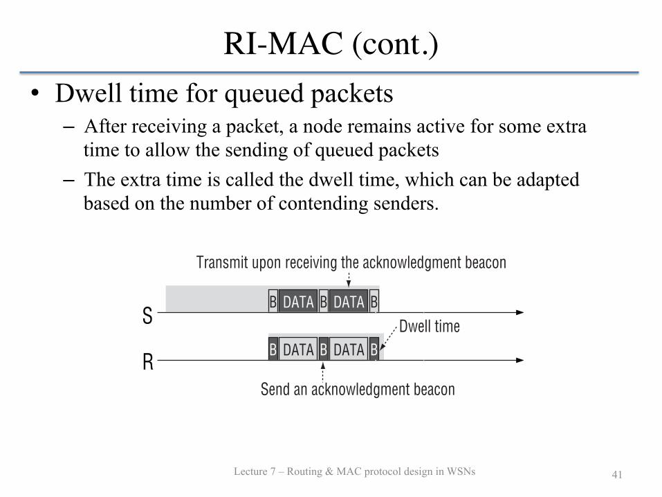
RI-MAC (cont.)


•  Dwell time for queued packets –  After receiving a packet, a node remains active for some extra

time to allow the sending of queued packets –  The extra time is called the dwell time, which can be adapted

based on the number of contending senders.

BDATA

DATA

B

B B

B

R

S

Node sends a beacon when it wakes up

Wake up to send and wait for beacon

Start data transmission upon receving R’s beacon

Node sends a beacon but goesto sleep since no incoming DATA

Figure 3: Overview of RI-MAC. Each node periodically wakesup and broadcasts a beacon. When node S wants to send aDATA frame to node R, it stays active silently and starts DATAtransmission upon receiving a beacon from R. Node S laterwakes up but goes to sleep after transmitting a beacon framesince there is no incoming DATA frame.

Hardware Preamble

Frame Length

FCF FCSSrc DstBW

RI-MAC-Specific

Figure 4: The format of an RI-MAC beacon frame for an IEEE802.15.4 radio. Dashed rectangles indicate optional fields. TheFrame Length, Frame Control Field (FCF), and Frame CheckSequence (FCS) are fields from IEEE 802.15.4 standard.

and X-MAC when the senders are hidden to each other, which canbe common in ad hoc sensor networks. As discussed in Section 3.4,after transmitting a beacon, a receiver detects collisions within theduration of the backoff window specified in the beacon, which ismuch shorter than the delay of a sleep interval needed in B-MACand X-MAC.RI-MAC also reduces overhearing, as a receiver expects incom-

ing data only within a small window after beacon transmission. To-gether with the lower cost for detecting collisions and recoveringlost DATA frames, RI-MAC achieves higher power efficiency, es-pecially when the network load increases. Even under light trafficload, which is the worst case for RI-MAC for power efficiency,RI-MAC still shows comparable performance to X-MAC in oursimulation and experimental evaluation onMICAzmotes. RI-MACstill decouples the sender’s and receiver’s duty cycle schedules asdo B-MAC and X-MAC, which removes the overhead of synchro-nization compared to synchronous duty cycle MAC protocols.

3.2. Beacon FramesA beacon frame in RI-MAC always contains a Src field, which isthe address of the source transmitting node of the beacon. We calla beacon with only a Src field a base beacon. A beacon can also in-clude two optional fields, depending on the roles the beacon serves:Dst, for destination address, and BW, for backoff window size. TheRI-MAC beacon frame format for an IEEE 802.15.4 radio is illus-trated in Figure 4 as an example.A node that receives a beacon can determine which fields are

present in the beacon by looking at the size of the beacon; with anIEEE 802.15.4 radio, size of a beacon is saved in the Frame Lengthfield. A beacon in RI-MAC can play two simultaneous roles: as anacknowledgment to previously received DATA, and as a request forthe initiation of the next DATA transmission, as illustrated in Fig-ure 5. After node R wakes up and senses clear medium, R transmitsa base beacon. If the medium is busy, R does a backoff and attemptsto transmit the beacon later. After receipt of the first DATA framefrom S in the figure, in the following beacon transmission by R, theDst field is set to S to indicate that this beacon also serves as theacknowledgment for the DATA received from S. Similar to ACK

BDATA

DATA

DATA

DATA

B B

B B BR

S

Transmit upon receiving the acknowledgment beacon

Send an acknowledgment beacon

Dwell time

Figure 5: The dual roles of a beacon in RI-MAC. A beaconserves both as an acknowledgment to previously received DATAand as a request for the initiation of the next DATA transmis-sion to this node.

transmission in IEEE 802.11, transmission of this acknowledgmentbeacon starts after SIFS delay, regardless of medium status. Nodesother than S ignore the Dst field in the beacon and treat it as a re-quest for the initiation of a new data transmission. The use of theBW field in a beacon is discussed in detail in Section 3.4.The duty cycle in RI-MAC is controlled by a parameter called

the sleep interval, which determines how often a node wakes upand generates a beacon to poll for pending DATA frames. Supposea sleep interval of L is used in some WSN. After a node generatesa beacon, the interval before the next beacon generation is set toa random value between 0.5×L and 1.5×L. In this way, we at-tempt to minimize the possibility that beacon transmissions fromtwo nodes become coincidentally synchronized.

3.3. Dwell Time for Queued PacketsAfter successfully receiving a DATA frame, a node remains activefor some extra time in order to allow queued packets to be sentto it immediately, as shown in Figure 5. We refer to this time asthe dwell time. Unlike in X-MAC, where the dwell time is set toa fixed value of the maximum backoff window, the dwell time inRI-MAC adapts to the number of contending senders. The durationof the dwell time is defined as the BW value from the last beaconplus SIFS and the maximum propagation delay. Since the BW ina beacon is automatically adjusted based on channel collisions ob-served by a node as discussed in detail next, so is the dwell time.The fewer contending senders and thus the fewer collisions, theshorter the dwell time. This self-adaptation helps RI-MAC usingthe shortest waiting time possible under light channel contentionwhile avoiding collisions under heavy channel contention.

3.4. DATA Frame Transmissions fromContending Senders

The challenges in handling transmissions from an unpredictablenumber of contending senders are twofold:

• minimize the active time of a receiver for power efficiency;and

• minimize the cost for collision detection and recovery of lostdata, whether or not senders are hidden to each other.

To meet these goals in RI-MAC, a receiver employs beaconframes to coordinate DATA frame transmissions from contendingsenders, as shown in Figure 6. The BW field in a beacon speci-fies the backoff window size senders should use when they contendfor the medium. If a received beacon does not contain a BW field(i.e., a base beacon), senders for this receiver should start transmit-ting DATA without backing off. If a beacon contains a BW field,each sender does a random backoff using the BW as the backoff

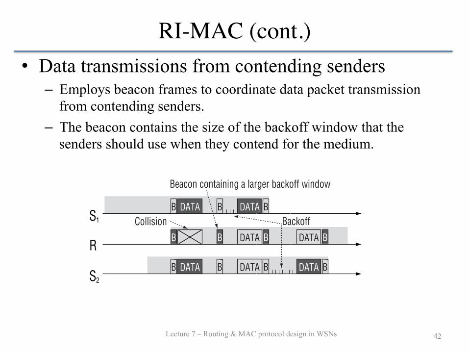
RI-MAC (cont.)


•  Data transmissions from contending senders –  Employs beacon frames to coordinate data packet transmission

from contending senders. –  The beacon contains the size of the backoff window that the

senders should use when they contend for the medium.

DATA DATA

DATA

DATA

DATA

DATA DATA

B B B

B BB B

B B B BR

S1

S2

Beacon containing a larger backoff window

Collision Backoff

Figure 6: DATA frame transmission from contending sendersin RI-MAC. For the first beacon, the receiver R requestssenders (here, S1 and S2) to start transmitting DATA imme-diately upon receiving the beacon. If a collision is detected, Rsends another beacon with increased BW value to request thatsenders do a backoff before their next transmission attempt.

window size over which to choose the actual backoff. The receiverincreases the value of the BW field upon detecting collisions.If a node cannot start data transmission as soon as it receives a

beacon, prior to actual DATA transmission, a sender should makesure that the medium has been idle for at least Tp time using CCA(clear channel assessment) checks. The CCA checks prevent asender from starting DATA transmission while the intended receiveris generating an acknowledgment beacon to a DATA frame just re-ceived from another sender. The time Tp here is set to SIFS plus themaximum propagation delay. If a node needs more time to generateand send an acknowledgment beacon, such as a software ACK usedin TinyOS, Tp should be increased correspondingly, as described inSection 3.8.After waking up, a node always broadcasts a base beacon with

no BW field. We made this design choice to optimize RI-MAC forthe most common cases of a typical WSN where there is light orno traffic most of the time. By enforcing all senders with pend-ing DATA frames to transmit immediately, we attempt to minimizetime for the node to determine whether or not there is incomingDATA. The shorter this duration, the less energy is used at eachwakeup. In this way, we attempt to minimize energy consump-tion if the network is idle most of the time. The duration can bevery short, as it is the the maximum round trip propagation delayplus radio switch delay (SIFS in IEEE 802.15.4). If the receiverdetects no channel activity within this duration, the receiver goesto sleep immediately. Although a base beacon could lead to con-current DATA transmissions to a same receiver, we found that theydo not necessarily lead to collisions in our experimental implemen-tation on MICAz motes [6], due to the presence of capture effectin the CC2420 radio [4]. This feature makes it possible for onesender to successfully transmit a packet to the receiver even if thetransmission overlaps with others, especially when senders havedifferent distances to the receiver (and thus different received sig-nal strengths) [16, 17].

3.5. Collision Detection and RetransmissionsBy coordinating DATA frame transmissions at receivers, RI-MACgreatly reduces the cost for detecting collisions and recovering lostDATA frames compared to B-MAC and X-MAC. As a sendercan transmit DATA frame only upon receiving a beacon, and sincethe backoff window size is explicitly controlled by the intendedreceiver, the receiver knows the maximum delay before a DATAframe’s arrival. This delay can be calculated from the BW valuein the previous beacon. The receiver need only detect the Startof Frame Delimiter (SFD) to learn of an incoming frame. Ifno SFD is detected in time, while some channel activity is de-tected by the CCA (clear channel assessment) check, the receiver

BDATA

DATAB

BB

B BR

S

Initial beacon

Beacon sent on request from S’s beacon

Figure 7: RI-MAC beacon-on-request. When node S wakes upfor transmitting a pending DATA frame, it sends a beacon withthe Dst field set to the destination of the pending DATA. If thedestination node R is already active, R in response transmits abeacon to enable S to begin DATA transmission immediately.

will decide that there was a collision and will generate anotherbeacon with a larger BW value. In RI-MAC, this new beaconis transmitted after the longest possible DATA transmission hasfinished so that all senders’ radios are already in receive mode.Prior to transmitting the beacon, a node does a random backoffto avoid possible repeated collisions with beacons from anothernode.After detecting a collision, a receiver calculates the new BW

value that will be used in the next beacon, by employing somebackoff strategy such as binary exponential backoff (BEB) in IEEE802.11 or Sift [14,21], depending on the density of a network. BEBis used in our implementation in TinyOS, as we found it adapts tonetworks of different densities and resolves collisions efficiently inRI-MAC in our evaluations.As RI-MAC initiates transmissions at the receiver, retransmis-

sion in RI-MAC is significantly different from that in sender-initiated approaches such as IEEE 802.11. In RI-MAC, a receiverplays the major role in retransmission control by managing the tim-ing and number of beacon transmissions. If the BW value hasreached the maximum backoff window size, or if the receiver keepsdetecting collisions after a number of consecutive beacon transmis-sions, the receive goes to sleep without further attempts. The cor-responding senders also become involved in retransmission con-trol, because a sender could miss receiving a beacon either be-cause of collisions or poor channel conditions. Thus, a sendermaintains a retry count for each DATA frame. If no beacon hasbeen received from the intended receiver within a time span 3times as long as the sleep interval, the sender increases the cur-rent retry count by 1. In addition, the sender increases this retrycount if no acknowledgment beacon is received within the maxi-mum backoff window after the sender transmitted a DATA framefollowing receipt of a beacon. When the retry count reaches a pre-defined retry limit, the sender cancels the transmission of the DATAframe.

3.6. Beacon-on-RequestIt is possible that the intended receiver node for some sender is al-ready active when the sender wakes up to transmit a DATA frameto it. An optimization, called beacon-on-request, is for this sender,after waking up for DATA transmission, to broadcast a beacon fol-lowing a CCA check, as illustrated in Figure 7. In this beacon, thesender S sets the Dst field to the receiver’s address, R. If the receiverR happens to be active, it generates a beacon in response after somerandom delay longer than the BW announced in the received bea-con from S. This beacon generated by the receiver on request ofthe sender allows the sender to transmit the pending DATA frameimmediately, rather than waiting until the next scheduled beacontransmission by R.

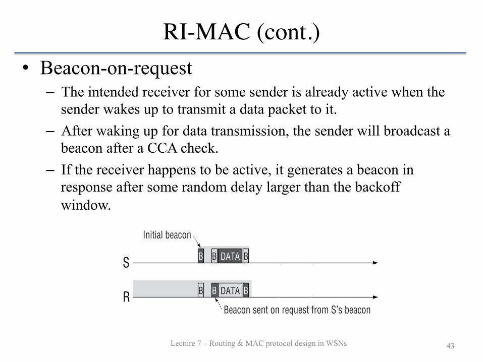
RI-MAC (cont.)


•  Beacon-on-request –  The intended receiver for some sender is already active when the

sender wakes up to transmit a data packet to it. –  After waking up for data transmission, the sender will broadcast a

beacon after a CCA check. –  If the receiver happens to be active, it generates a beacon in

response after some random delay larger than the backoff window.

DATA DATA

DATA

DATA

DATA

DATA DATA

B B B

B BB B

B B B BR

S1

S2

Beacon containing a larger backoff window

Collision Backoff

Figure 6: DATA frame transmission from contending sendersin RI-MAC. For the first beacon, the receiver R requestssenders (here, S1 and S2) to start transmitting DATA imme-diately upon receiving the beacon. If a collision is detected, Rsends another beacon with increased BW value to request thatsenders do a backoff before their next transmission attempt.

window size over which to choose the actual backoff. The receiverincreases the value of the BW field upon detecting collisions.If a node cannot start data transmission as soon as it receives a

beacon, prior to actual DATA transmission, a sender should makesure that the medium has been idle for at least Tp time using CCA(clear channel assessment) checks. The CCA checks prevent asender from starting DATA transmission while the intended receiveris generating an acknowledgment beacon to a DATA frame just re-ceived from another sender. The time Tp here is set to SIFS plus themaximum propagation delay. If a node needs more time to generateand send an acknowledgment beacon, such as a software ACK usedin TinyOS, Tp should be increased correspondingly, as described inSection 3.8.After waking up, a node always broadcasts a base beacon with

no BW field. We made this design choice to optimize RI-MAC forthe most common cases of a typical WSN where there is light orno traffic most of the time. By enforcing all senders with pend-ing DATA frames to transmit immediately, we attempt to minimizetime for the node to determine whether or not there is incomingDATA. The shorter this duration, the less energy is used at eachwakeup. In this way, we attempt to minimize energy consump-tion if the network is idle most of the time. The duration can bevery short, as it is the the maximum round trip propagation delayplus radio switch delay (SIFS in IEEE 802.15.4). If the receiverdetects no channel activity within this duration, the receiver goesto sleep immediately. Although a base beacon could lead to con-current DATA transmissions to a same receiver, we found that theydo not necessarily lead to collisions in our experimental implemen-tation on MICAz motes [6], due to the presence of capture effectin the CC2420 radio [4]. This feature makes it possible for onesender to successfully transmit a packet to the receiver even if thetransmission overlaps with others, especially when senders havedifferent distances to the receiver (and thus different received sig-nal strengths) [16, 17].

3.5. Collision Detection and RetransmissionsBy coordinating DATA frame transmissions at receivers, RI-MACgreatly reduces the cost for detecting collisions and recovering lostDATA frames compared to B-MAC and X-MAC. As a sendercan transmit DATA frame only upon receiving a beacon, and sincethe backoff window size is explicitly controlled by the intendedreceiver, the receiver knows the maximum delay before a DATAframe’s arrival. This delay can be calculated from the BW valuein the previous beacon. The receiver need only detect the Startof Frame Delimiter (SFD) to learn of an incoming frame. Ifno SFD is detected in time, while some channel activity is de-tected by the CCA (clear channel assessment) check, the receiver

BDATA

DATAB

BB

B BR

S

Initial beacon

Beacon sent on request from S’s beacon

Figure 7: RI-MAC beacon-on-request. When node S wakes upfor transmitting a pending DATA frame, it sends a beacon withthe Dst field set to the destination of the pending DATA. If thedestination node R is already active, R in response transmits abeacon to enable S to begin DATA transmission immediately.

will decide that there was a collision and will generate anotherbeacon with a larger BW value. In RI-MAC, this new beaconis transmitted after the longest possible DATA transmission hasfinished so that all senders’ radios are already in receive mode.Prior to transmitting the beacon, a node does a random backoffto avoid possible repeated collisions with beacons from anothernode.After detecting a collision, a receiver calculates the new BW

value that will be used in the next beacon, by employing somebackoff strategy such as binary exponential backoff (BEB) in IEEE802.11 or Sift [14,21], depending on the density of a network. BEBis used in our implementation in TinyOS, as we found it adapts tonetworks of different densities and resolves collisions efficiently inRI-MAC in our evaluations.As RI-MAC initiates transmissions at the receiver, retransmis-

sion in RI-MAC is significantly different from that in sender-initiated approaches such as IEEE 802.11. In RI-MAC, a receiverplays the major role in retransmission control by managing the tim-ing and number of beacon transmissions. If the BW value hasreached the maximum backoff window size, or if the receiver keepsdetecting collisions after a number of consecutive beacon transmis-sions, the receive goes to sleep without further attempts. The cor-responding senders also become involved in retransmission con-trol, because a sender could miss receiving a beacon either be-cause of collisions or poor channel conditions. Thus, a sendermaintains a retry count for each DATA frame. If no beacon hasbeen received from the intended receiver within a time span 3times as long as the sleep interval, the sender increases the cur-rent retry count by 1. In addition, the sender increases this retrycount if no acknowledgment beacon is received within the maxi-mum backoff window after the sender transmitted a DATA framefollowing receipt of a beacon. When the retry count reaches a pre-defined retry limit, the sender cancels the transmission of the DATAframe.

3.6. Beacon-on-RequestIt is possible that the intended receiver node for some sender is al-ready active when the sender wakes up to transmit a DATA frameto it. An optimization, called beacon-on-request, is for this sender,after waking up for DATA transmission, to broadcast a beacon fol-lowing a CCA check, as illustrated in Figure 7. In this beacon, thesender S sets the Dst field to the receiver’s address, R. If the receiverR happens to be active, it generates a beacon in response after somerandom delay longer than the BW announced in the received bea-con from S. This beacon generated by the receiver on request ofthe sender allows the sender to transmit the pending DATA frameimmediately, rather than waiting until the next scheduled beacontransmission by R.

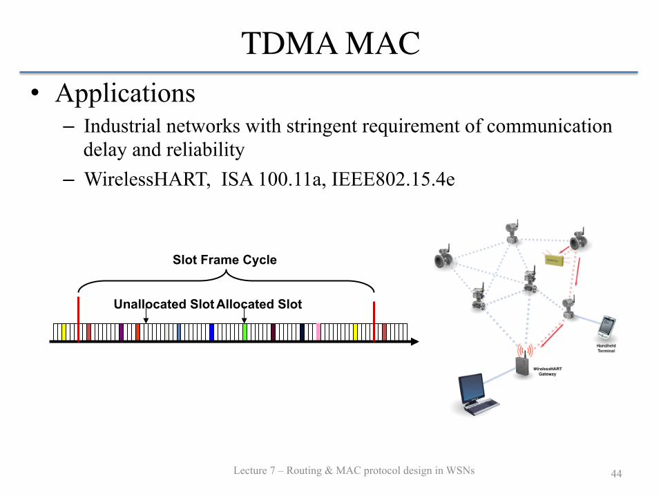
TDMA MAC


•  Applications –  Industrial networks with stringent requirement of communication

delay and reliability –  WirelessHART, ISA 100.11a, IEEE802.15.4e

Slot Frame Cycle

Unallocated Slot Allocated Slot

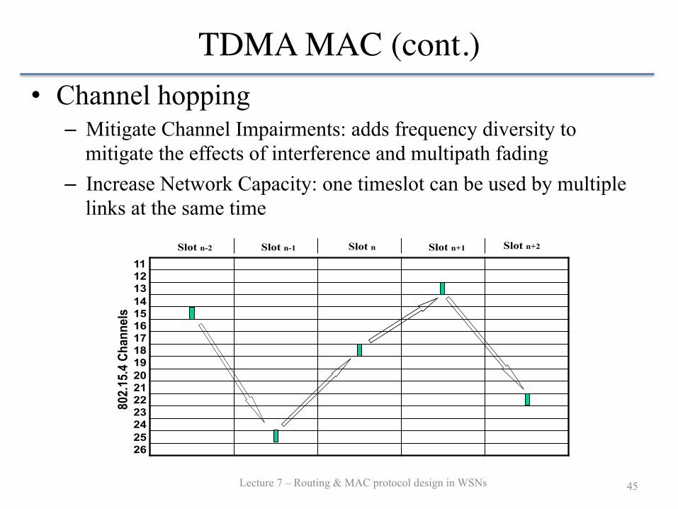
TDMA MAC (cont.)


•  Channel hopping –  Mitigate Channel Impairments: adds frequency diversity to

mitigate the effects of interference and multipath fading –  Increase Network Capacity: one timeslot can be used by multiple

links at the same time doc.: IEEE 802.15-08-0581-02-004e

Submission

September, 2008

Kris Pister et al. Slide 12

Channel Hopping

•  Combined with timeslot access to enhance reliability

11 12 13 14 15 16 17 18 19 20 21 22 23 24 25 26

802.

15.4

Cha

nnel

s

Slot n Slot n-1 Slot n-2 Slot n+1 Slot n+2

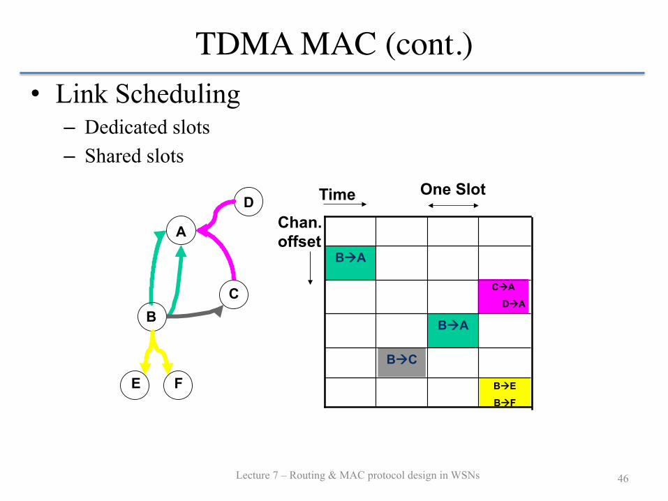
TDMA MAC (cont.)


•  Link Scheduling –  Dedicated slots –  Shared slots

doc.: IEEE 802.15-08-0581-02-004e

Submission

September, 2008

Kris Pister et al. Slide 14

B!A

B!C

B!A

C!A

D!A

B!E

B!F

B C

Link = (Timeslot , Channel Offset)

A

Time

Chan. offset

One Slot D

•  The two links from B to A are dedicated •  D and C share a link for transmitting to A •  The shared link does not collide with the dedicated links

F E

Documents

Lecture 7 Overview - University of Otago · Lecture 7 Overview • Last Lecture ... • Routing protocol design in Contiki – Communication architecture in Contiki – Rime communication