Lecture Notes #12: MANOVA & Canonical Correlation 12-1gonzo/coursenotes/file12.pdf · I will now use our new knowledge of matrix manipulations to show how a simple formulation can

Lecture Notes #12: MANOVA & Canonical Correlation 12-1

Richard GonzalezPsych 614Version 2.7 (Mar 2017)

LECTURE NOTES #12: MANOVA & Canonical Correlation

Reading Assignment

T&F chapters (or the J&W chapter) on MANOVA and canonical correlation.

1. Review of repeated-measures ANOVA

Last semester we covered repeated-measures ANOVA. I emphasized my preferencefor testing contrasts over omnibus tests. Recall that omnibus tests in the context ofrepeated measures are difficult to conduct because there is much “pooling” that needsto occur in order to compute an error term. That is, in order to have a single errorterm for all tests, one needs to make sure that there is homogeneity of variances (acrossgroups and variables) and a kind of homogeneity of covariances (also across groupsand variables). In order to do that amount of pooling we had to make additionalassumptions like compound symmetry.

Instead of all that pooling to compute a single error term, we opted for a techniquethat allowed each contrast to have its own error term, thus eliminating the need topool across time periods to create an error term. We called that the “multivariateapproach” to repeated measures (Maxwell & Delaney devoted two chapters to thetraditional pooling approach and two chapters to the newer multivariate approach).You should review the lecture notes on repeated measures from last semester beforecontinuing.

I will now use our new knowledge of matrix manipulations to show how a simpleformulation can handle any contrast in any ANOVA design (though here I’ll just showa special case of the more general formulation). The results of the present section areidentical to what we did last semester (i.e., either creating new variables with thecompute command or directly in MANOVA). This exercise will help to reinforcesome of the new material we’ve learned this semester, and set the stage for how wewill handle multivariate ANOVA.

First, we need to define some terms. Let X be a matrix of means arranged so thatgroups go along the rows and variables go along the columns. For example, the two-sample t test has two means (one for each group) and corresponds to an X with tworows and one column. There is one column because in the classic example there isonly one dependent variable.


Group Time 1

1 X11

2 X21

A second example: the paired t test has two means (one for each time) and correspondsto an X with one row and two columns. There is one row because there is one group.

Group Time 1 Time 2

1 X11 X12

A third example: a 2 (within) × 2 (between) ANOVA consists of X with two columns(repeated times) and two rows (two groups).

Group Time 1 Time 2

1 X11 X12

2 X21 X22

Let lowercase “a” denote a contrast on the within-subject variables, and lowercase“c” denote a contrast on between-subject variables. We’ll adopt a convention that allcontrasts are column vectors.

The contrast value I can be written as

I = ctXa (12-1)

where the superscript t denotes the transpose. Be sure you understand this equationand how it relates to I from previous lectures.

If there is only one variable then a is the contrast (1) and I is the usual∑

cti X. When

there is only one group the contrast c is (1) and I reduces to∑

Xa. The conceptualadvantage of the present system is that it can handle both between-subjects andwithin-subjects contrasts simultaneously.

Next, we need an error term. Recall that last semester we had the MSE term playthe role of error. Now, because we have more than one variable, we need an MSEmatrix. This matrix is a square matrix and has as many rows (and columns) asthere are variables. It looks much like a correlation matrix but instead of containingcorrelations it contains MSEs along the diagonal and cross-variable MSEs everywhereelse. It is pooled over groups, so the usual equality of variance assumption over groupsis made but there will be no pooling over variables. I’ll call this MSE matrix S.


The computation of matrix S is not easy. SPSS prints a related matrix as part ofthe output from MANOVA as the SSCP error matrix (if you want to use this matrix,you’ll need to divide the SSCP matrix in the MANOVA output by the error degreesof freedom to get the matrix S). Matrix S contains the relevant information in termsof what the right error term should be (e.g., as needed for nested effects and randomeffects).

The standard error of I can be expressed as√√√√(∑ c2

ni

)atSa (12-2)

Finally, one can divide I by its standard error and test the result using a t distributionwith N - (number of groups) degrees of freedom.

A student and I wrote a short SPSS macro that implements this matrix formulationof contrasts. It yields identical results to the MANOVA command. Feel free to useit, though we don’t guarantee it is bug free. The code and instructions on how to useit are posted on the class web site.

I implemented a similar idea in R but it still needs some work. See the canvas site,ganova-tutorial.Rmd file (and corresponding html output file) if you are interested.The point is that one can do complex contrasts with a very simple interface: specifythe repeated measures contrast a and the between-subjects contrast b and you’re done.

If you know how to program (whether it be in a language like pascal or C, or know yourway around a spreadsheet program like Excel), it may be a good learning experienceto program this general contrast formulation yourself. If you do a lot of contrasts onwithin-subjects designs in your research, you may find it useful too, much easier torun contrasts than using the SPSS MANOVA or GLM command or trying to figureout how to do this in R (recall the extremely long appendix in LN5 illustrating halfa dozen ways to do this in R and the careful attention that needs to be paid in orderto get each one of those approaches done correctly).

SPSS now has a built in feature as part of GLM that allows you to implement these twotypes of contrasts (between-subjects and within-subjects). It is called the LBM=Kcustom hypotheses. The L matrix is the contrasts on the between subjects, the Mmatrix is the contrast within subjects, B are estimates, and K are the hypothesizedconstants (usually set to zero in most null hypothesis settings).

You can say for example


GLM dv BY iv1 iv2

/method = sstype(3)

/intercept = include

/LMATRIX ’levels of iv1 at each level of iv2’

iv1 1 -1 iv1*iv2 1 -1 0 0 0 0 ;

iv1 1 -1 iv1*iv2 0 0 1 -1 0 0 ;

iv1 1 -1 iv1*iv2 0 0 0 0 1 -1

/print = test(lmatrix)

/design iv1 iv2 iv1*iv2

This set of contrasts is decomposing the sum of squares for each pair of iv1 comparisonsat each level of iv2. For output you’ll get a print out of the LMATRIX, an omnibustest for all contrasts listed in the LMATRIX (unfortunately it is called a “contrast”even though it can be made up of multiple single degree of freedom contrasts), andseparate tests for each line in the LMATRIX syntax. Apparently, SPSS requires thatboth the main effect contrast “iv1” and its corresponding higher order interaction“iv1*iv2” be included in order to run. I haven’t played around too much with differentways of writing this command. The documentation is pretty sketchy and I don’t findthe syntax very intuitive.

Similarly, you can specify contrasts over repeated measures using the MMATRIX andyou can set specific values of the null hypothesis using the KMATRIX (the default iszero).

So far, this section on comparisons in both repeated measures and between subjectsANOVA focuses on specific “single degree of freedom” comparisons (aka contrasts).If you need to do omnibus tests, things get tricky as we saw in Lecture Notes 5 be-cause we need to aggregate over multiple contrasts. If each contrast has a differenterror term, then a combined error term over multiple contrasts doesn’t make muchsense. Recall there are two basic approaches: one involves pooling the error matrixand one that specifies a unique error for every test. Within each of these basic ap-proaches there are some variants, such as within the pooling approach one could use aGreenhouse-Geisser correction and within the separate variance approach one can usea multivariate approach or a random effects approach, different types of estimationroutines like maximum likelihood, etc.

We now return to the multivariate approach to repeated measures ANOVA that Ibriefly presented in Lecture Notes 5. Given our new knowledge of PCA and linearalgebra (Lecture Notes 11) as well as the contrast logic I introduced in the previoussection of these lecture notes we can gain a deeper understanding about the multi-variate approach.


2. Multivariate ANOVA

(a) Overview: MANOVA as a procedure for omnibus tests

One feature of multivariate ANOVA is that it provides a way to test omnibus testsin the context of repeated measures without making as stringent assumptions.

The (silly) standard“textbook logic” for MANOVA involves cases where you havemultiple dependent variables and an ANOVA-type design. The story goes likethis. (1) You first run a MANOVA to get the “mother of all omnibus tests” in thesense that the test is corrected for multiple measures and multiple groups. (2)If the MANOVA is significant, then you have the green light to run individualomnibus tests on each dependent variable. (3) If the ANOVAs on the individualdependent variables are significant, then you have the green light to run individ-ual contrasts on each dependent variable. If at any point a test is not significantyou stop. Just like the kid’s game of green light, red light.

By now you know how I feel about omnibus tests, so I won’t go into a discussionof their limitations here. Let’s just say that there may be a time in your careerwhere you may be forced to run an omnibus test on a repeated measures design.If so, you have two options. You can go the route of correcting degrees of freedomin a Welch-like way (these were the Greenhouse-Geisser and Hyndt-Feldt testswe discussed last semester). Or you can run a multivariate ANOVA, which hasa better way of aggregating the error term over all the measures. Aficionadosof omnibus tests tend to prefer the multivariate ANOVA over the Welch-likecorrections. But, can we really trust the opinions of those who advocate omnibustests. . . ? So, if you can avoid omnibus tests and just do contrasts on repeatedmeasures variables, you’ll be much better off.

It turns out that there is another use of multivariate ANOVA, which I find morepalatable and may turn out to be quite useful in your research.

(b) MANOVA as a way to find an optimal contrast over variables (aka PCA marriesANOVA)

For me, the usefulness of a multivariate ANOVA is that it provides optimal “con-trast” weights for the dependent variables. That is, it provides a way of findingthe “best” contrast possible over the dependent variables. One can then inter-pret this optional contrast to see which variables are related to group differences.As we will see, these optimal weights lead to new variables that are interpretedmuch like components in a PCA. So multivariate ANOVA computed in the wayadvocated in this subsection of the lecture notes amounts to a hybrid of PCA


with ANOVA, a way of comparing components across groups.

The basic idea is similar to the intuition underlying Scheffe’s observation thatthere exists a “maximum” contrast that has a sum of squares that is identicalto SSB, even when SSB has more than one degree of freedom. Scheffe’s resultapplies to a contrast over groups, it turns out there is an analogous contrast overvariables that is also “maximal” in the sense that it gives the best way to linearlyweight the variables in order to maximize the significance test associated withthe contrast. As we will see later, this “maximal” contrast also has a Scheffe-likecorrection associated with it.

In order to get the intuition of a maximal contrast over variables I need to developsome of the pieces. It turns out that this maximal contrast is equivalent to thefirst eigenvector that falls out of a natural matrix in the ANOVA context (sortof a “PCA meets ANOVA” B movie).

First, we need the matrix analog of SSB (sum of squares between) and SSW(sum of squares within).

Recall that at the beginning of these lecture notes we used “a” to refer to acontrast on within-subject factors. In the case of a within-subjects factor, the“a” represented contrasts selected by the analyst to test a linear hypothesis overvariables. MANOVA extends this logic by computing the optimal contrast “a”that best weights the variables. As we will see, this contrast “a” will be aneigenvector. So, in a within-subjects ANOVA the researcher selects the contrast,whereas in MANOVA, the algorithm selects the contrast.

The F test for this eigenvector “a” is given by

F (a) =atHa

atEa

N − pp− 1

(12-3)

where p is the number of variables, a is the eigenvector of a new matrix E−1H(which is intuitively SSB/SSW in matrix terms), E is the SSCP error matrix, His the SSCP hypothesis matrix (SSCP stands for “sum of square cross products”),and N is the sample size. The degrees of freedom for the F test are (p, N-p).The F test examines whether the optimal way to linearly combine the variablesyields an I that is statistically significant.

The SSCP error matrix E is the matrix analog of SSW and the SSCP hypothesismatrix H is the matrix analog of SSB in an ANOVA. The usual SSW and SSBfor each individual variable are along the diagonals of the E and H matrix,respectively. The off-diagonals represent the cross-product terms (i.e., cross-variable terms). The term E−1H is the matrix analog of SSB/SSW, which is one


of the important ingredients in constructing the F test, as we saw in the ANOVAsection of the course.

Example. Here is an actual data set with 10 variables (a standard measure ofself-esteem). There were 252 male and female participants. Each participantresponded on a four point scale to each of the 10 items below.

i. At times I think I am no good at all.

ii. I take a positive view of myself.

iii. All in all, I am inclined to feel that I am a failure.

iv. I wish I could have more respect for myself.

v. I certainly feel useless at times.

vi. I feel that I am a person of worth, at least on an equal plane with others.

vii. On the whole, I am satisfied with myself.

viii. I feel that I do not have much to be proud of.

ix. I feel that I have a number of good qualities.

x. I am able to do things as well as most other people.

Some questions are worded positively (i.e., “I am good”) whereas others areworded negatively (i.e., “I am bad”)–we’ll come back to this later. For eachof the 10 questions subjects responded a number 0, 1, 2 or 3, depending on theiragreement to the statement.

The first 10 variables in the data set are responses to these 10 questions, codedfrom 0-3 where 0 represents strongly disagree, 1 represents mildly disagree, 2represents mildly agree and 3 represents strongly agree. In addition, the sex ofthe subject is also coded (1=female, 2=male).

To save time and space, I omit the descriptive statistics. Normally, the 20 means(10 variables by 2 sexes) should be printed in a table or a figure. Assumptionswere checked and everything looked fine: normality, equal variance across sexesfor each variable, linearity in scatterplots for all combinations of variables (sep-arately by sex), and independence.

data list free/v01 v02 v03 v04 v05 v06 v07 v08 v09 v10 sex.

begin data0 2 0 0 0 2 2 0 3 3 12 2 1 2 2 2 2 1 2 1 10 2 0 2 2 3 2 0 3 3 12 2 0 0 2 3 3 1 2 2 10 2 0 1 0 2 2 0 2 2 1


2 3 0 0 2 3 3 1 3 2 1[LOTS MORE DATA]end data.

manova v01 v02 v03 v04 v05 v06 v07 v08 v09 v10 by sex(1,2)/discrim all alpha(1).

EFFECT .. SEX

Multivariate Tests of Significance (S = 1, M = 4 , N = 119 1/2)

Test Name Value Exact F Hypoth. DF Error DF Sig. of F

Pillais .02470 .61029 10.00 241.00 .805

Hotellings .02532 .61029 10.00 241.00 .805

Wilks .97530 .61029 10.00 241.00 .805

Roys .02470

Note.. F statistics are exact.

EFFECT .. SEX (Cont.)

Univariate F-tests with (1,250) D. F.

Variable Hypoth. SS Error SS Hypoth. MS Error MS F Sig. of F

V01 .25979 215.21243 .25979 .86085 .30179 .583

V02 .07055 82.83024 .07055 .33132 .21294 .645

V03 .63497 114.32931 .63497 .45732 1.38847 .240

V04 .00417 205.24583 .00417 .82098 .00508 .943

V05 .63497 188.04360 .63497 .75217 .84418 .359

V06 .00742 88.70686 .00742 .35483 .02091 .885

V07 .09091 106.33766 .09091 .42535 .21373 .644

V08 .24536 101.00464 .24536 .40402 .60730 .437

V09 .01670 81.84045 .01670 .32736 .05101 .822

V10 .17940 116.05473 .17940 .46422 .38645 .535


Raw discriminant function coefficients

Function No.

Variable 1

V01 .49375

V02 .45937

V03 .81825

V04 .03137

V05 -.87960

V06 -.17763

V07 .31953

V08 .63413

V09 -.50816

V10 .70854


Standardized discriminant function coefficients

Function No.

Variable 1

V01 .45811

V02 .26442

V03 .55334

V04 .02842

V05 -.76286

V06 -.10581

V07 .20839

V08 .40307


V09 -.29075

V10 .48275

Estimates of effects for canonical variables

Canonical Variable

Parameter 1

2 -.16256

Correlations between DEPENDENT and canonical variables

Canonical Variable

Variable 1

V01 .21833

V02 .18340

V03 .46832

V04 -.02834

V05 -.36517

V06 -.05748

V07 .18374

V08 .30972

V09 -.08976

V10 .24707

First, look at the multivariate tests of significance. These report omnibus testsover the 10 variables of males vs. females. No statistically significant resultwas observed. The omnibus F test was .61. The test on the best statisticalfooting is Wilk’s test (it is based on the likelihood ratio test). The Pillais testis based on the Lagrangian multiplier test, and Roy’s test is based on the Waldtest. In this particular example, all the tests produced the identical F test,but in general they will not always agree. When they disagree, I’d believe theWilk’s test over the others. Another difference is that Roy’s test focuses onlyon the first eigenvector whereas the others pool over all possible eigenvectors.Pillai appears to be more robust to violations of normality and homogeneity ofcovariance but the appropriateness of which test to choose under which situationis not well-understood. How all these tests differ and in tests are best under whatconditions are open research questions.

After the multivariate tests, the output presents univariate tests on each vari-able separately. In the present example, these univariate tests are identical toperforming a two-sample t test separately on each of the 10 variables. Make sureyou understand this!

Some people worry about the multiplicity problem with all those univariate tests,so they devised a little scheme. Run the multivariate test. If that is significant,then go on to the separate univariate tests. Otherwise, stop because the omnibus


multivariate wasn’t significant. By this logic we would not look at the individualtwo sample t tests in this example because the omnibus test was not significant.

The SPSS output lists “s, m and N”. These are defined as follows:

s = min(T-1, p)

m =|T − p| − 1

2

N =number of subjects− T − p− 1

2

where T is number of groups and p is number of variables. When s = 1, then allthree multivariate tests are equivalent and are distributed as F.

What I want to show, however, is the usual information present in the SPSSoutput, which suggests an interesting way to interpret the results of MANOVA.Immediately after the univariate tests, there is a section labelled the “raw dis-criminant function coefficients”. This is the first eigenvector of the matrix E−1Hthat I discussed above. It tells you how to weight the variables to create a newsingle variable. Note that this is analogous to the factor score coefficient matrixprinted in principal components. The eigenvector can be interpreted as a setof weights and thus provides information about which variables distinguish thegroups. For example, by looking at the eigenvector in the above example we seethat some variables had weights very close to zero (relative to other variables), sowe know that those variables probably would not be related to any sex differenceshad there been a significant sex effect.

The next part of the output lists discriminant function coefficients for standard-ized variables (i.e., if all your variables were standardized to Z-scores). This latteroutput may be easier to interpret than the “raw coefficients” when the variablesthemselves are on different scales. The raw coefficients are obviously influencedby scale and so you need to be mindful of scale when interpreting the raw coeffi-cients. The standardized coefficients have been purged of scale. We saw this lastsemester in the context of regression (raw beta or standardized beta) and also inPCA where we looked at either the factor score coefficient matrix or the factormatrix.

The last part of the output presents the correlations between the individualvariables and the “factor scores” created with the raw weights. This matrix ofcorrelations is analogous to the “components matrix” in the PCA output. Aswith PCA, some people prefer interpreting these correlations rather than thecoefficients themselves.

Actually, these are not simple correlations but partial correlations using the


grouping variable as the variable that is partialled out (recall partial correla-tions from an earlier regression lecture). You can double check this by manuallycreating the factor score by multiplying the raw coefficient weights by each vari-able and summing to create a new factor score. Then correlate the new factorscore with each variable using the SPSS partial correlation program with sex ofsubject as the control variable. The rationale is that these correlations shouldbe independent from differences between group means.

Here I illustrate this partial correlation. First, compute the variable newvar,which is the weights sum of the 10 observed variables.

compute newvar = .4937*V01 + .4593*V02 + .8182*V03 + .03137*V04 - .8796*V05 -

.17763*V06 + .3195*V07 + .634*V08 - .50816*V09 + .70854*V10.

execute.

PARTIAL CORR

/VARIABLES= v01 v02 v03 v04 v05 v06 v07 v08 v09 v10 newvar BY sex

/SIGNIFICANCE=TWOTAIL

/MISSING=LISTWISE .

This syntax will produce an 11x11 correlation matrix. If you look at the par-tial correlations between the variable newvar and each of the individual observedvariables you will see that the partial correlations are identical to the MANOVAoutput that prints the correlations between the dependent and canonical vari-ables.

How are these coefficients related to the rest of the analyses? These coefficientsproduce what can be thought of as “factor scores” from a PCA, and the F testin this example tests the mean factor scores for the men against the mean factorscores for the women. I will verify this by example. Create a new variable usingthe raw score coefficients as weights. This is just like performing a contrast, onlythe contrast weights aren’t determined by the analyst in advance but instead areestimated from the data.

compute newvar = .4937*V01 + .4593*V02 + .8182*V03 + .03137*V04 - .8796*V05 -

.17763*V06 + .3195*V07 + .634*V08 - .50816*V09 + .70854*V10.

execute.

[OUTPUT OF TWO-SAMPLE T-TEST]

Number

Variable of Cases Mean SD SE of Mean

-----------------------------------------------------------------------

NEWVAR

SEX 1 154 1.7315 .979 .079

SEX 2 98 2.0566 1.032 .104


-----------------------------------------------------------------------

Mean Difference = -.3251

Levene’s Test for Equality of Variances: F= .860 P= .355

t-test for Equality of Means 95%

Variances t-value df 2-Tail Sig SE of Diff CI for Diff

-------------------------------------------------------------------------------

Equal -2.52 250 .012 .129 (-.580, -.071)

Unequal -2.49 198.57 .014 .131 (-.583, -.067)

-------------------------------------------------------------------------------

This t-test (t=2.52 for the pooled test) suggests a significant difference betweenmen and women on this “factor score”. Why didn’t the previous MANOVAfind a statistically significant result? The reason is that the t test I just ranis not completely correct because it hasn’t been corrected for the estimation of10 coefficient weights. The MANOVA p-value has been corrected in a Scheffe-like way for the “fishing expedition” that the computer went on to find the bestpossible contrast (the raw score coefficients) that produced the best t possiblebetween men and women.

It turns out that the t and F above are related to each other in a relatively simpleway. Letting t denote the t computed directly on the “factor scores” and F be the(corrected) F test printed in the MANOVA output, we have this relationship:

F =(N1 +N2 − p− 1)

p(N1 +N2 − 2)t2 (12-4)

In this formula, the Ni refers to the sample size in group i, and p refers to thenumber of items. The degrees of freedom for this F test are p and (N1−N2−p−1).The term that multiplies t2 is not dependent on how your data turn out–once youpick sample size and number of variables, the constant of proportionality thatrelates F and t2 is determined. In this sense, we can think of Equation 12-4 asa correction of the t test to take into account the “data mining” that went on tofind the weights1. This correction is due to Hotelling. The correction factor willalways be less than or equal to 1 so the effect when multiplying t2 is to reduce itsvalue. Convention requires that when you perform a one-sample or two-samplet test with lots of variables, you call it a “Hotelling’s T” in honor of the guy2.

1When there is only one sample, the relevant formula for relating the one sample t test and the MANOVAis the following equation instead of Equation 12-4:

F =(N − p)

p(N − 1)t2

where the F has (p, N-P) degrees of freedom.2There is a relationship between Wilk’s test and Hotelling’s test: W = (1+(T2/N-1))−N/2. Thus, Wilk

and Hotelling are, in some sense, related.


Entering the numbers for the data set from the current example yields

F =(252− 10− 1)

10(252− 2)2.522

=241

10 ∗ 2502.522

= .0964 ∗ 2.522

= .6122

which is identical (within roundoff error) to the multivariate F test printed in theMANOVA output. Note that regardless of what t is observed between the sexeson the factor score, for this sample size and number of variables the corrected Fwill only be 9.64% the size of t2. The correction is quite large in this example.

(c) Verifying optimized t value

This next subsection verifies that the set of weights computed in the MANOVAcommand optimizes the t-test. I’ll do this in R because it has a nice optimizationroute. First, I read in the self-esteem data and assign variable names. Second,I’ll run the manova command in R to illustrate we reproduce the basic outputfrom SPSS reported earlier (e.g., same Hotelling’s T2, same coefficients). Third,I’ll set up the maximization function and find the set of weights that producethe maximum possible t-value; also show that the optimization function findsthe maximum t-value at 2.52 as did SPSS’ MANOVA command. Fourth, I’llplot the two sets of weights (manova and optimization) to show they are linearlyrelated and have a correlation of 1, meaning they are the same up to a lineartransformation.

> #set paths and read data

> setwd("/users/gonzo/rich/Teach/multstat/unixfiles/lectnotes/manova")

> data <- read.table("selfest.dat", header=F)

> #set matrix and assign variable names

> data <- as.matrix(data)

> names(data) <- c(paste("v",1:10,sep=""), "sex")

> #run manova in R

> out.manova <- manova(data[,1:10] ~ data[,11])

> summary(out.manova)

Df Pillai approx F num Df den Df Pr(>F)

data[, 11] 1 0.024698 0.61029 10 241 0.8045

Residuals 250

> #extract coefficients (weights) from out.manova using candisc

> library(candisc)

> coeff.manova <- candisc(out.manova)$coeffs.raw

> coeff.manova


Can1

V1 0.49375240

V2 0.45936937

V3 0.81824584

V4 0.03137036

V5 -0.87959886

V6 -0.17762553

V7 0.31952943

V8 0.63412815

V9 -0.50816159

V10 0.70853908

> #run optimization to find weights that maximize the t value

> #function to optimize

> manova.t <- function(w) {

+ weight.sum <- data[,-11] %*% w

+ abs(t.test(weight.sum ~ data[,11], var.equal=T)[[1]])

+ }

> #fnscale negative makes it into a maximation problem

> out.optim <- optim(rep(1,10), manova.t,

+ control=list(fnscale=-1), method="CG")

> out.optim

$par

[1] 1.34797915 1.25408761 2.23388023 0.08564688 -2.40137931 -0.48493230

[7] 0.87237073 1.73124543 -1.38727380 1.93433961

$value

[1] 2.516104

$counts

function gradient

121 61

$convergence

[1] 0

$message

NULL

> #plot both sets of coefficients and show they are linearly related and

> #corr = 1

> par(pty="s")

> plot(coeff.manova, out.optim$par, xlab="manova coefficients",

+ ylab="optimization coefficients")

> abline(lm(out.optim$par ~ coeff.manova))

> cor(out.optim$par, coeff.manova)

Can1

[1,] 1


●●

●

●

●

●

●

●

●

●

−0.5 0.0 0.5

−2

−1

01

2

manova coefficients

optim

izat

ion

coef

ficie

nts

(d) The multivariate normality assumption turns out to be very important for thesetests. The corrections are based on the assumption holding, so if the usualstatistical assumptions don’t hold, then the test can be meaningless. Keep inmind that the equality of variance assumptions must hold too. If there are groupdifferences, you’ll be pooling variances. Plus, for the covariance matrices tomake any sense, all the scatterplots between variables within each group shouldbe linear (recall this point from Lecture Notes #6.

(e) As I mentioned above, some people believe the reason one runs a MANOVA isto serve as a gigantic omnibus test. When you have several variables and severalgroups you will likely perform lots of tests. This worries some people for thereasons we discussed last semester so they play the “green light, red light” game.

This is quite silly. The real scoop is that it depends on what was planned andwhat wasn’t, and, as argued last semester, what can be replicated. Considerthis 2 × 3 arrangement of possibilities (inspired by an idea suggested by Harris,1985): you either plan or perform post hoc comparisons on the between-subjects


factors and you either plan or perform post hoc comparisons or estimate linearcombinations on the within-subjects factors, where by “estimate” I mean the useof the eigenvector approach for the within contrast rather than an experimenterchosen contrast like we did last semester in repeated measures ANOVA.

Within-Subjects

Between-Subjects Planned Post-hoc Estimated by data

Planned

Post-hoc

Filling in this table is not straightforward. The simpler cells are, for instance, thecell where contrasts on both the between and within-subject factors are planned–in that cell one would probably not worry about corrections for multiple contrasts(especially if replication were possible, as I argued in the ANOVA section of thiscourse). The “estimated by data” column under within-subjects refers to caseswhere one runs MANOVA over the repeated measures to find optimal contrastweights over the variables. In this case a multivariate correction is needed. Ithink this is a useful way to organize the various possibilities. Now we need moreresearch to figure out what to do in any given cell of that table.

(f) The assumptions of a multivariate ANOVA parallel those of ANOVA—equalvariances across groups and normally distributed residuals. Some types of viola-tions of independence can be handled through repeated measures and time seriesmodels in the context of MANOVA.

The multivariate normal distribution is denoted as N with mean vector µ andcovariance matrix

∑. The covariance matrix has the variance in the diagonal

(e.g,. the variance of variable 1 in row/column 1, the variance of variable 2in row/column 2, etc) and covariances in the off-diagonal. We saw examples ofmultivariate normal distributions (with two variables) at the beginning of lecturenotes #6.

An example of a null hypothesis tested in MANOVA is as follows. Suppose wehave two groups and four variables, and want to test the null hypothesis thatthere is a difference between the four means.

Ho: µ11µ21µ31µ41

=

µ12µ22µ32µ42

(12-5)

The alternative hypothesis is that the means are not equal. Compare this to the


simple case in Lecture Notes #1 with two groups on just one variable

Ho: (µ11

)=

(µ12

)The difference is merely in the number of dependent variables.

(g) Relation between repeated measures ANOVA and MANOVA

In Lecture Notes 5 I presented repeated measures ANOVA. At the beginning ofthe present lecture notes I showed a simple way to test contrasts (both within-subjects and between-subjects) using the matrix notation introduced in the pre-vious lecture notes. Now I want to make a connection with the matrix notationwe developed for single degree of freedom tests and omnibus tests.

To illustrate I’ll use the example of a one-way repeated measures ANOVA inMaxwell and Delaney. Data for 8 subjects are listed:

t1 t2 t3

[1,] 2 3 5

[2,] 4 7 9

[3,] 6 8 8

[4,] 8 9 8

[5,] 10 13 15

[6,] 3 4 9

[7,] 6 9 8

[8,] 9 11 10

Suppose we want to test the linear (-1, 0 ,1) and quadratic (1,-2,1) contrastsover the three levels of time. We could use the framework I introduced at thebeginning of these lecture notes using matrix algebra to test each of the twoseparate contrasts over time. Those would each be single tests (with N - 1 = 7degrees of freedom for error) and could be tested as is without any correction.That is identical to the output you would get from running either the MANOVAor GLM command, with each contrast having its own error term, such as

GLM t1 t2 t3

/WSFACTOR=time 3 Polynomial

/WSDESIGN=time.

Tests of Within-Subjects Contrasts


ANOVA SOURCE TABLE FOR EACH TEST OF LINEAR AND QUAD

Source SS df Mean Square F Sig.time Linear 36.000 1 36.000 15.750 .005Quad 1.333 1 1.333 1.273 .296Error Linear 16.000 7 2.286Quad 7.333 7 1.048

The GLM command (as does the MANOVA command) reports both types ofomnibus tests. One type assumes equal error across all contrasts in order tocombine the contrasts into a single omnibus test. This is the test that can becorrected with either Greenhouse-Geisser or Huynh-Feldt. The omnibus testsstarts off with 2 degrees of freedom in the numerator (one for each contrast)and 14 degrees of freedom in the denominator (twice as many as each of the twoindividual contrasts). The corrections merely serve to reduce the denominatordegrees of freedom. The second type of test is also printed, the multivariate testthat does not assume equal variances across the two contrasts in order to pool.This test allows each contrast to have its own error variance, and also models thecovariance between the two contrasts. The same GLM command also producesthis output

Multivariate Tests

Test Value F Ndf Ddf Sig.Pillai’s Trace .865 19.148 2.000 6.000 .002Wilks’ Lambda .135 19.148 2.000 6.000 .002Hotelling’s 6.383 19.148 2.000 6.000 .002Roy’s Largest 6.383 19.148 2.000 6.000 .002

I’ll use the new language and tools we have just developed to illustrate how themultivariate approach to the omnibus test in repeated measures works. The restof this subsection will get technical, especially with linear algebra. No need toworry if you don’t understand the details. I care more about the big pictureand that you understand that PCA and ANOVA are used together to addressomnibus question about differences between groups with multiple measures.

The multivariate repeated measures omnibus test emerges by computing the Hand E matrices as described above for MANOVA. The E matrix is the error sumof squares cross products that is equivalent to the covariance matrix of the threemeasures times the quantity N - 1. The H matrix is the sum of squares of thedata matrix (t(data) * data where * denotes matrix multiplication) minus the Ematrix. Both H and E are 3x3 matrices. Now define the matrix of contrasts thathas two columns (one for each contrast, linear and quadratic) and three rows


(one for each measure); call that CMAT.

We need to create an F test similar in form to Equation 12-3, where the H andthe E matrices are each multiplied by a single contrast a. We will use the resultthat eigenvectors represent the optimal weights to create the omnibus test thatcombines across several contrasts. First, create versions of H and E that arepre and post multiplied by CMAT, so HC = t(CMAT) * H * CMAT and EC= t(CMAT) * E * CMAT. Find the eigenvector of the matrix (EC)−1(HC), andthen apply that eigenvector to H and E as per Equation 12-3. The EC andHC versions are used only to compute the eigenvector, which can be thought ofas optimally combining the information of both contrasts into a single contrastthat carries the same information (recall Scheffe’s result mentioned in LectureNotes 3 that a single contrast can equal the entire sum of squares between forthe omnibus test). In R this is done with these two lines of syntax, the first linecomputes the first eigenvector and the second line uses that eigenvector in a formsimilar to Equation 12-3:

large.root <- eigen(solve(EC) %*% HC)$vectors[,1]

fnew <- ((t(large.root) %*% H %*% large.root) /

(t(large.root) %*% E %*% large.root)) *

((nrow(data) - ncol(data)+1)/(ncol(data)-1))

The value of fnew in this example will be 19.148 as per the GLM output.

An alternate way to compute the same multivariate omnibus F test is to usethe approach in Maxwell and Delaney’s book. The error for the full model EFis based on the E matrix by pre and most multiplying E by the CMAT matrixthat contains both contrasts. The error for the reduced model ER is based onthe H matrix by pre and post multiplying M by the CMAT contrast, where Mis the matrix of sum of squares from the raw data or t(data) * data, where *denotes matrix multiplication and t() refers to transpose. One then computesthe determinant of each of ER and EF and plugs those two terms into a formulafor the F test that compares the reduction in error between the full and reducedmodels. Below is the R syntax that also produces an f value equal to 19.148(for details see Maxwell and Delaney’s chapter on the multivariate approach torepeated measures ANOVA).

cmat <- cbind(c(-1,0,1),c(1,-2,1))

EF <- t(cmat)%*%E%*%cmat

M <- t(data) %*% data

ER <- t(cmat) %*% M %*% cmat

f <- (det(ER) - det(EF))/det(EF) * (nrow(data) - ncol(data)+1)/ (ncol(data)-1)

critf <- qf(.95,ncol(data)-1,nrow(data)-ncol(data)+1)


The key point to make is that the multivariate approach to repeated-measuresANOVA computes error on each contrast separately and then combines each ofthose separate error terms into a single omnibus tests. There are two equivalentways to approach the computation (one is through the eigenvector and anotheris through the determinant). This differs from the other approach to omnibusrepeated measures tests, which assumes structure on the covariance matrix overtime and uses the same error term for all contrasts to construct the omnibus test.

One last tidbit before moving on to another topic. What is the difference betweendoing a regular multivariate analysis and a repeated measures ANOVA using themultivariate approach. In other words, what is the difference between these twoways to call the MANOVA command:

manova t1 t2 t3

/wsfactor time (3)

/wsdesign.

manova t1 t2 t3

/discrim raw stand.

The first version treats time as a factor with three levels and imposes two orthog-onal contrasts, whereas the second version treats the three time measures as threeseparate dependent variables. The former imposes a structure (contrasts) thatthe latter does not. The former tests an omnibus question over two contrasts, thelatter tests the optimal combination on the three variables (three measurementsover time). The latter is what we did in the previous section when I introducedMANOVA as a test over multiple measures. If we perform Equation 12-3 di-rectly on the sum of squares cross product matrices (without imposing contrastson those sum of squares cross products), then we test the optimal combinationof the three times. The F test for this example is 19.92 with 3 (number of mea-sures) degrees in the numerator and 5 (N - number of measures) degrees in thedenominator. The difference in the approaches boils down to whether the matrixCMAT (the matrix of contrasts) is applied to the sum of squares cross productterms.

3. Canonical Correlation

Suppose you have two sets of variables and you want to know how to optimally com-bine (in a linear manner) each set so that the correlation between the two combinationsis maximum. That is, you want to find a linear combination of set1 and a linear com-bination of set2 such that the correlation of the two linear combinations is maximal.The “maximal” part comes in as a way to define the weights, that is, as a criterion


that helps determine the two sets of weights.

You probably have already inferred that we’ll convert this into an eigenvalue problem.In essence, we find a separate eigenvector for set1, a separate eigenvector for set2,use the eigenvectors to create new scores (analogous to “factor scores” in the PCAworld), and then correlate the two factor scores. All this is done simultaneouslyso that all pieces in the analyses are “informed” of all other pieces. The theory ofcanonical correlation shows that there are no other linear combinations of the twosets of variables that will produce a better correlation.

The theory relies heavily on linear algebra so I won’t go into the details here. For thoseinterested in the mathematical development of canonical correlation, see Johnson andWichern who give the appropriate matrix formulas.

(a) CANCORR MACRO

SPSS doesn’t have a built in canonical correlation procedure, but it does supplya macro for computing one. You can find the macro in the directory where SPSSis stored (e.g., on a PC it is usually ‘‘c:\Program Files\SPSS’’ ). The fileappears in different names for different versions, but is usually called a variant of“cancorr.sps” or “canonical correlation.sps”. To run the macro, you need to typethis into the syntax window:

include file "PATH-TO-CANCOR"

where PATH-TO-CANCOR is the directory path on your machine to the filecancorr.sps. PC users may need to start SPSS “as administrator” in order forSPSS to have permission to write the intermediate files that the macro produces.

Here is an example using the self-esteem data set. I will compute a canonical cor-relation between the five positively worded items and the five negatively wordeditems. A graphical depiction of what we are doing is presented in Figure 12-1.

include file "c:\Program Files\Spss\Canonical correlation.sps".

cancorr set1 = V01 V03 V04 V05 V08

/set2 = V02 V06 V07 V09 V10.

Correlations for Set-1

V01 V03 V04 V05 V08

V01 1.0000 .3627 .3031 .4980 .3820

V03 .3627 1.0000 .3401 .3625 .3916

V04 .3031 .3401 1.0000 .3875 .3139


Figure 12-1: Graphical illustration of canonical correlation on the five positive and fivenegative items for the self-esteem data.

V 01 V 02

V 03 V 06

V 04 F1

``

gg

oo

ww

~~

ks +3 F2

>>

77

//

''

V 07

V 05 V 09

V 08 V 10

V05 .4980 .3625 .3875 1.0000 .3853

V08 .3820 .3916 .3139 .3853 1.0000

Correlations for Set-2

V02 V06 V07 V09 V10

V02 1.0000 .3579 .5777 .3616 .3610

V06 .3579 1.0000 .4308 .4057 .4560

V07 .5777 .4308 1.0000 .3245 .3753

V09 .3616 .4057 .3245 1.0000 .6173

V10 .3610 .4560 .3753 .6173 1.0000

Correlations Between Set-1 and Set-2

V02 V06 V07 V09 V10

V01 -.4076 -.2664 -.3423 -.2297 -.2772

V03 -.2174 -.2157 -.2499 -.2260 -.2316

V04 -.3891 -.2334 -.4229 -.2739 -.2671

V05 -.3106 -.2424 -.3382 -.2477 -.3117

V08 -.3647 -.4379 -.4094 -.4229 -.3741

Canonical Correlations

1 .647

2 .251

3 .130

4 .110

5 .007


Test that remaining correlations are zero:

Wilk’s Chi-SQ DF Sig.

1 .530 156.076 25.000 .000

2 .910 23.147 16.000 .110

3 .971 7.191 9.000 .617

4 .988 2.981 4.000 .561

5 1.000 .011 1.000 .916

Standardized Canonical Coefficients for Set-1

1 2 3 4 5

V01 -.274 .660 .961 -.061 -.136

V03 .024 -.209 -.240 -.234 -1.086

V04 -.409 .527 -.518 .746 .053

V05 -.108 .055 -.601 -.957 .485

V08 -.570 -.887 .255 .255 .327

Raw Canonical Coefficients for Set-1

1 2 3 4 5

V01 -.295 .712 1.038 -.066 -.146

V03 .035 -.309 -.355 -.346 -1.605

V04 -.452 .582 -.572 .825 .058

V05 -.124 .064 -.693 -1.104 .559

V08 -.897 -1.397 .401 .402 .515

Standardized Canonical Coefficients for Set-2

1 2 3 4 5

V02 .334 -.785 -.837 -.099 .399

V06 .225 .670 -.723 .008 -.645

V07 .400 -.176 .993 -.351 -.606

V09 .255 .639 .238 -.729 .805

V10 .129 -.192 .260 1.293 .118

Raw Canonical Coefficients for Set-2

1 2 3 4 5

V02 .581 -1.366 -1.457 -.172 .695

V06 .379 1.127 -1.216 .013 -1.085

V07 .614 -.270 1.526 -.539 -.931

V09 .446 1.119 .417 -1.276 1.410

V10 .190 -.282 .382 1.901 .173

Canonical Loadings for Set-1

1 2 3 4 5

V01 -.661 .432 .516 -.299 -.147

V03 -.477 -.118 -.185 -.249 -.814

V04 -.705 .398 -.461 .358 -.067

V05 -.614 .170 -.311 -.685 .170

V08 -.835 -.531 .134 .006 .053

Cross Loadings for Set-1

1 2 3 4 5

V01 -.427 .108 .067 -.033 -.001

V03 -.309 -.030 -.024 -.027 -.005

V04 -.456 .100 -.060 .039 .000

V05 -.397 .043 -.041 -.075 .001

V08 -.540 -.133 .017 .001 .000

Canonical Loadings for Set-2


1 2 3 4 5

V02 .784 -.486 -.342 -.095 .152

V06 .679 .485 -.380 .115 -.383

V07 .821 -.206 .373 -.156 -.348

V09 .676 .451 .125 -.077 .564

V10 .660 .158 .148 .680 .237

Cross Loadings for Set-2

1 2 3 4 5

V02 .507 -.122 -.045 -.010 .001

V06 .439 .122 -.050 .013 -.003

V07 .531 -.052 .049 -.017 -.002

V09 .437 .113 .016 -.008 .004

V10 .426 .040 .019 .075 .002

Redundancy Analysis:

Proportion of Variance of Set-1 Explained by Its Own Can. Var.

Prop Var

CV1-1 .447

CV1-2 .134

CV1-3 .125

CV1-4 .150

CV1-5 .144

Proportion of Variance of Set-1 Explained by Opposite Can.Var.

Prop Var

CV2-1 .187

CV2-2 .008

CV2-3 .002

CV2-4 .002

CV2-5 .000

Proportion of Variance of Set-2 Explained by Its Own Can. Var.

Prop Var

CV2-1 .528

CV2-2 .148

CV2-3 .088

CV2-4 .103

CV2-5 .133

Proportion of Variance of Set-2 Explained by Opposite Can. Var.

Prop Var

CV1-1 .221

CV1-2 .009

CV1-3 .001

CV1-4 .001

CV1-5 .000

There are lots of matrices in this output. First, the usual Pearson correlationmatrices within a set and across sets is printed.


Then the canonical correlations are printed. For example, the first canonicalcorrelation is .647. This is the best correlation we can attain by correlating anylinear combination of set1 with any linear combination of set2. In this example,there are a total of five canonical correlations (one correlation for each pair ofeigenvectors, and there are as many eigenvector pairs as there are variables in aset). The second best linear combination that is orthogonal to the first produces acorrelation of .251 between the two sets. Thus, each pair of eigenvectors produceslinear combinations that are orthogonal to the other linear combinations. Thegeneral logic is analogous to forming a set of 5 orthogonal contrasts on set1 andfive orthogonal contrasts on set2, then finding the correlations between the 5pairs. The key is that the weights are defined to a) maximize the correlation andb) be orthogonal to each other.

The number of possible canonical correlations is equal to the number of variablesin the smaller of the two sets. That is, if set1 has k variables and set2 has lvariables, then the maximum number of canonical correlations that are possibleis min(k,l).

Then we have the test of significance for the canonical correlations. These are“corrected” for the weights that need to be estimated within a correlation, butare not corrected for tests on multiple canonical correlations. In other words,they correct for the fishing expedition in finding the best set of linear weightsfor a single canonical correlation, but not for the fact that in this example weperformed five fishing expeditions.

Then we have the standardized and raw coefficients for each set. These corre-spond to the raw and standardized “factor score coefficient matrices” we saw inPCA. They tell us how to weight the raw (or standardized) variables to createthe “factor scores.” They correspond to eigenvectors. To illustrate, if I took thefirst column of raw coefficients for set1 and used them as weights to create a newweighted sum of the variables in set1, did the same for set2 using the first columnof raw coefficients for set2, and then correlated these two weighted sums I wouldget a correlation of .647, the first canonical correlation. We can interpret theweights to get an understanding of how the .647 came to be, i.e., which variablescontributed most heavily to the weighted sums.

Finally, we have the canonical loadings. These are analogous to the “factormatrix” in PCA. They correspond to the correlation between the raw variablesand the “factor scores” as computed by using the eigenvectors as weights.

The redundancy stuff in the SPSS output is a little confusing. See T&F page205-207 for an explanation. Intuitively, it has to do with the how much varianceone canonical variable accounts for a set and there are various possibilities for


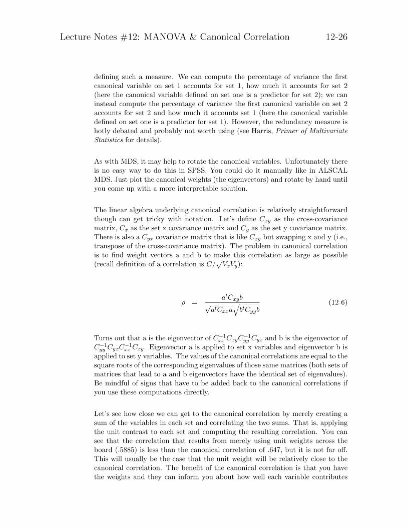
defining such a measure. We can compute the percentage of variance the firstcanonical variable on set 1 accounts for set 1, how much it accounts for set 2(here the canonical variable defined on set one is a predictor for set 2); we caninstead compute the percentage of variance the first canonical variable on set 2accounts for set 2 and how much it accounts set 1 (here the canonical variabledefined on set one is a predictor for set 1). However, the redundancy measure ishotly debated and probably not worth using (see Harris, Primer of MultivariateStatistics for details).

As with MDS, it may help to rotate the canonical variables. Unfortunately thereis no easy way to do this in SPSS. You could do it manually like in ALSCALMDS. Just plot the canonical weights (the eigenvectors) and rotate by hand untilyou come up with a more interpretable solution.

The linear algebra underlying canonical correlation is relatively straightforwardthough can get tricky with notation. Let’s define Cxy as the cross-covariancematrix, Cx as the set x covariance matrix and Cy as the set y covariance matrix.There is also a Cyx covariance matrix that is like Cxy but swapping x and y (i.e.,transpose of the cross-covariance matrix). The problem in canonical correlationis to find weight vectors a and b to make this correlation as large as possible(recall definition of a correlation is C/

√VxVy):

ρ =atCxyb

√atCxxa

√btCyyb

(12-6)

Turns out that a is the eigenvector of C−1xx CxyC

−1yy Cyx and b is the eigenvector of

C−1yy CyxC

−1xx Cxy. Eigenvector a is applied to set x variables and eigenvector b is

applied to set y variables. The values of the canonical correlations are equal to thesquare roots of the corresponding eigenvalues of those same matrices (both sets ofmatrices that lead to a and b eigenvectors have the identical set of eigenvalues).Be mindful of signs that have to be added back to the canonical correlations ifyou use these computations directly.

Let’s see how close we can get to the canonical correlation by merely creating asum of the variables in each set and correlating the two sums. That is, applyingthe unit contrast to each set and computing the resulting correlation. You cansee that the correlation that results from merely using unit weights across theboard (.5885) is less than the canonical correlation of .647, but it is not far off.This will usually be the case that the unit weight will be relatively close to thecanonical correlation. The benefit of the canonical correlation is that you havethe weights and they can inform you about how well each variable contributes


to the construct. With that information you may be better able to create newindices based on unit weights.

compute sumset1 = V01 + V03 + V04 + V05 + V08.compute sumset2 = V02 + V06 + V07 + V09 + V10.execute.

correlate sumset1 sumset2.

- - Correlation Coefficients - -

SUMSET1 SUMSET2

SUMSET1 1.0000 .5884

( 252) ( 252)

P= . P= .000

SUMSET2 .5884 1.0000

( 252) ( 252)

P= .000 P= .

To illustrate how well the canonical coefficients can help pick out variables, let’slook at the resulting correlation from merely using the variables that have thehighest weights. Because the variables are on the same scale, I’ll use the rawweights (but one should be careful because if variables are on different scales thenthe standardized coefficients will be easier to interpret). For the first canonicalvariable, the raw weights for set 1 suggest that variables 4 and 8 are the primarycontributors with weights-.452 and -.897, respectively. Similarly, the raw weightssuggest that variables 2 and 7 are both the relatively high on weights (.581 and.614, respectively). Let’s look at the correlation of just these four variables (i.e.,the correlation of the two sums).

compute subset1 = V04 + V08.compute subset2 = V02 + V07.execute.

correlate subset1 subset2.

SUBSET1 SUBSET2

SUBSET1 1.0000 .5501

( 252) ( 252)

P= . P= .000

SUBSET2 .5501 1.0000

( 252) ( 252)

P= .000 P= .

Here the correlation is .55 which is clearly not as good as the canonical correlation(which is based on the optimal weights whereas here we forced three variables


in each set to have weights of 0 and two variables to have weights of 1). Butnevertheless, we sacrifice relatively little and have a more parsimonious quantityto interpret: a correlation of two sums, each sum based on two variables.

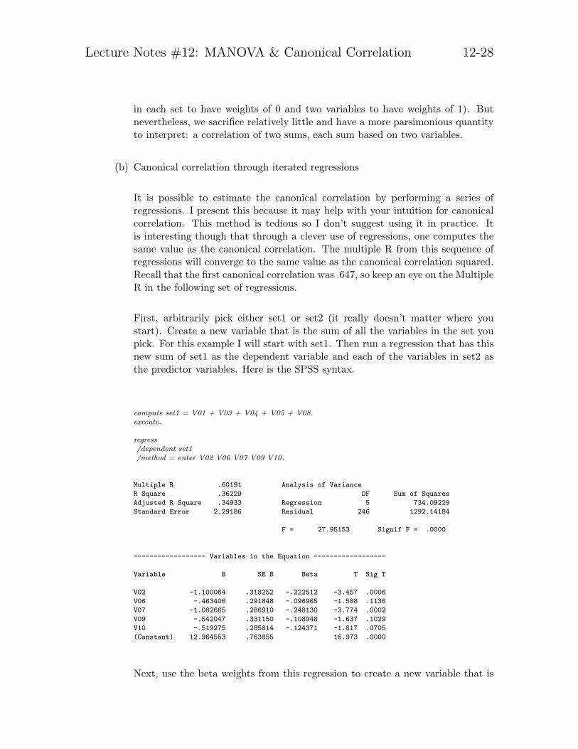
(b) Canonical correlation through iterated regressions

It is possible to estimate the canonical correlation by performing a series ofregressions. I present this because it may help with your intuition for canonicalcorrelation. This method is tedious so I don’t suggest using it in practice. Itis interesting though that through a clever use of regressions, one computes thesame value as the canonical correlation. The multiple R from this sequence ofregressions will converge to the same value as the canonical correlation squared.Recall that the first canonical correlation was .647, so keep an eye on the MultipleR in the following set of regressions.

First, arbitrarily pick either set1 or set2 (it really doesn’t matter where youstart). Create a new variable that is the sum of all the variables in the set youpick. For this example I will start with set1. Then run a regression that has thisnew sum of set1 as the dependent variable and each of the variables in set2 asthe predictor variables. Here is the SPSS syntax.

compute set1 = V01 + V03 + V04 + V05 + V08.execute.

regress/dependent set1/method = enter V02 V06 V07 V09 V10.

Multiple R .60191 Analysis of Variance

R Square .36229 DF Sum of Squares

Adjusted R Square .34933 Regression 5 734.09229

Standard Error 2.29186 Residual 246 1292.14184

F = 27.95153 Signif F = .0000

------------------ Variables in the Equation ------------------

Variable B SE B Beta T Sig T

V02 -1.100064 .318252 -.222512 -3.457 .0006

V06 -.463406 .291848 -.096965 -1.588 .1136

V07 -1.082665 .286910 -.248130 -3.774 .0002

V09 -.542047 .331150 -.108948 -1.637 .1029

V10 -.519275 .285814 -.124371 -1.817 .0705

(Constant) 12.964553 .763855 16.973 .0000

Next, use the beta weights from this regression to create a new variable that is


the weighted sum of the set2 variables. I could have just saved the fits from thatregression but to illustrate what is going on I will compute the weighted sumdirectly with a COMPUTE command. Then, run a second regression with thenew weighted sum of set2 as the dependent variable and each of the set1 variablesas predictors. This regression will give you new weights to use for set1 variables.

compute set2 = -1.1*V02 - .4634*V06 - 1.082*V07 - .542*V09 - .51927*V10 + 12.96.execute.





Standard Error 1.32063 Residual 246 429.04083

F = 34.94107 Signif F = .0000



V01 .343574 .108586 .186185 3.164 .0018

V03 -.043364 .142392 -.017165 -.305 .7610

V04 .511638 .103989 .270603 4.920 .0000

V05 .151191 .118773 .076669 1.273 .2042

V08 .939866 .152454 .349134 6.165 .0000

(Constant) 3.037414 .172558 17.602 .0000

Repeat this process several times until you converge. That is, take the resultsfrom the current regression, save the fitted values (i.e., the Y hats). Run asubsequent regression with those fitted values as the dependent variable and thevariables from the other set as the predictor variables. Here I illustrate with twomore rounds.

compute set1 = .3436*V01 - .0434*V03 + .5116*V04 + .1512*V05 + .9399*V08 + 3.037.execute.





Standard Error .84919 Residual 246 177.39808


F = 35.30610 Signif F = .0000



V02 -.423350 .117921 -.220822 -3.590 .0004

V06 -.260182 .108137 -.140391 -2.406 .0169

V07 -.439435 .106308 -.259709 -4.134 .0000

V09 -.308277 .122700 -.159784 -2.512 .0126

V10 -.139219 .105902 -.085986 -1.315 .1899

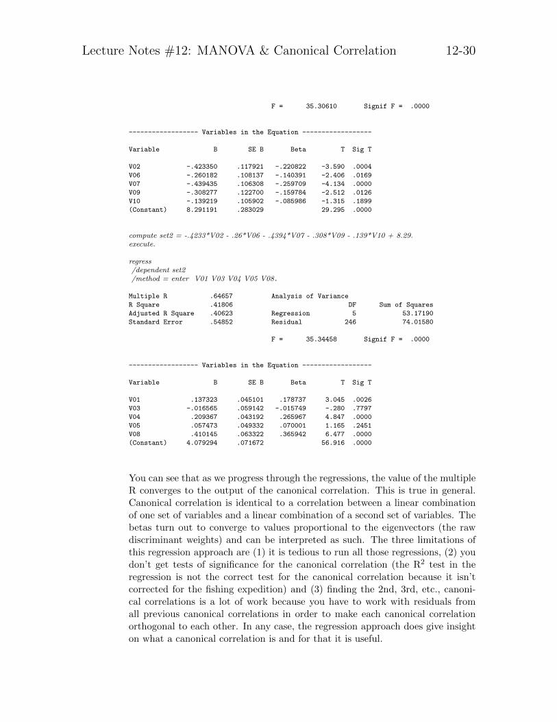
(Constant) 8.291191 .283029 29.295 .0000

compute set2 = -.4233*V02 - .26*V06 - .4394*V07 - .308*V09 - .139*V10 + 8.29.execute.





Standard Error .54852 Residual 246 74.01580

F = 35.34458 Signif F = .0000



V01 .137323 .045101 .178737 3.045 .0026

V03 -.016565 .059142 -.015749 -.280 .7797

V04 .209367 .043192 .265967 4.847 .0000

V05 .057473 .049332 .070001 1.165 .2451

V08 .410145 .063322 .365942 6.477 .0000

(Constant) 4.079294 .071672 56.916 .0000

You can see that as we progress through the regressions, the value of the multipleR converges to the output of the canonical correlation. This is true in general.Canonical correlation is identical to a correlation between a linear combinationof one set of variables and a linear combination of a second set of variables. Thebetas turn out to converge to values proportional to the eigenvectors (the rawdiscriminant weights) and can be interpreted as such. The three limitations ofthis regression approach are (1) it is tedious to run all those regressions, (2) youdon’t get tests of significance for the canonical correlation (the R2 test in theregression is not the correct test for the canonical correlation because it isn’tcorrected for the fishing expedition) and (3) finding the 2nd, 3rd, etc., canoni-cal correlations is a lot of work because you have to work with residuals fromall previous canonical correlations in order to make each canonical correlationorthogonal to each other. In any case, the regression approach does give insighton what a canonical correlation is and for that it is useful.


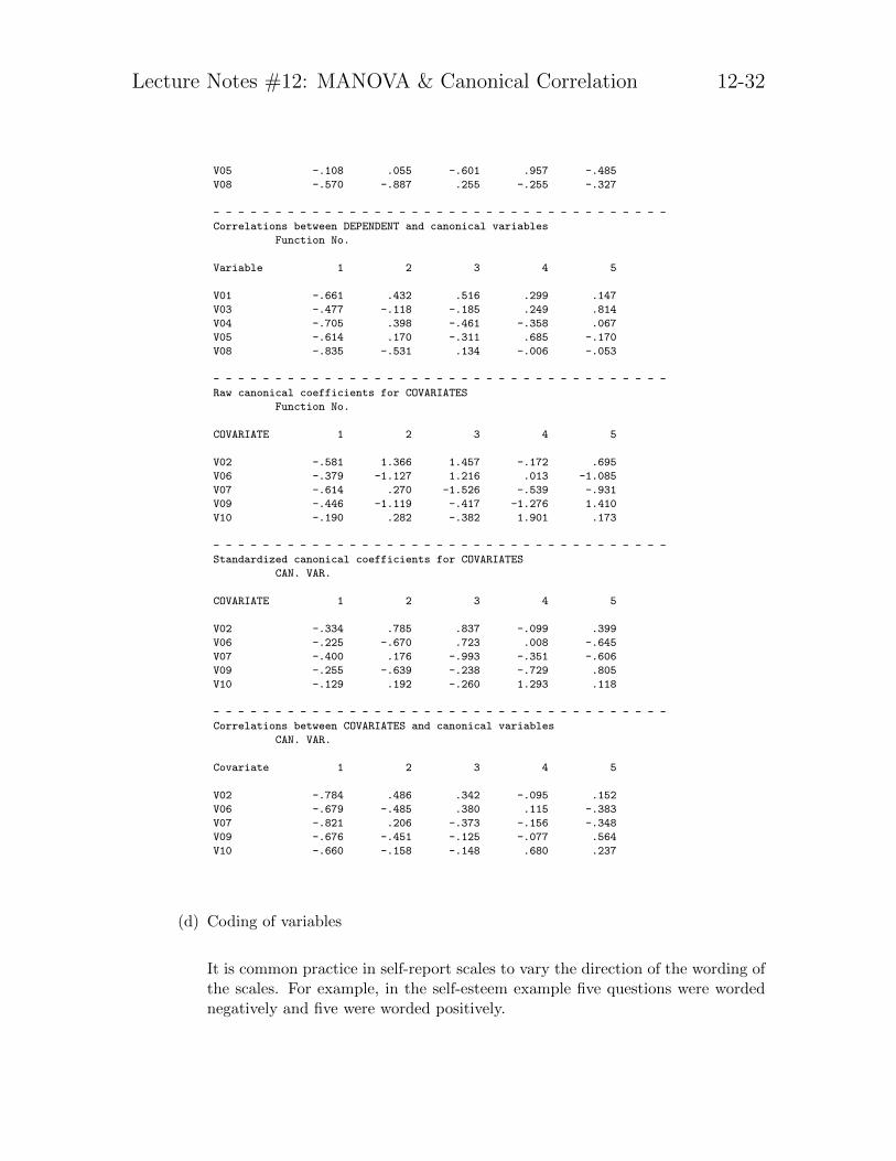
(c) Canonical Correlation through the MANOVA command

It is possible to run a canonical correlation through the MANOVA command.The key word WITH separates the two sets of variables.

manova x1set1 x2set1 x3set1 WITH x1set2 x2set2 x3set2

/discrim all alpha(1)

/print=sig(eigen dim).

alpha(1) instructs SPSS to print out all canonical correlations. The output in-cludes the raw canonical coefficients, which are the weights used to create thecanonical variables.

Here are excerpts from the resulting output. You can see that it is identicalto using the cancor macro, except for occasional complete sign reversals, whichwill not change the interpretation of the results. In the output one set is labelled“dependent”and the other set is labelled“covariate”. I omitted a bunch of outputwhere each “dependent variable” is regressed on the “covariate variables”.

Eigenvalues and Canonical Correlations

Root No. Eigenvalue Pct. Cum. Pct. Canon Cor. Sq. Cor

1 .719 88.142 88.142 .647 .418

2 .067 8.238 96.379 .251 .063

3 .017 2.122 98.501 .130 .017

4 .012 1.493 99.994 .110 .012

5 .000 .006 100.000 .007 .000

- - - - - - - - - - - - - - - - - - - - - - - - - - - - - - - - - - - - -

Raw canonical coefficients for DEPENDENT variables

Function No.

Variable 1 2 3 4 5

V01 -.295 .712 1.038 .066 .146

V03 .035 -.309 -.355 .346 1.605

V04 -.452 .582 -.572 -.825 -.058

V05 -.124 .064 -.693 1.104 -.559

V08 -.897 -1.397 .401 -.402 -.515

- - - - - - - - - - - - - - - - - - - - - - - - - - - - - - - - - - - - -

Standardized canonical coefficients for DEPENDENT variables

Function No.

Variable 1 2 3 4 5

V01 -.274 .660 .961 .061 .136

V03 .024 -.209 -.240 .234 1.086

V04 -.409 .527 -.518 -.746 -.053


V05 -.108 .055 -.601 .957 -.485

V08 -.570 -.887 .255 -.255 -.327

- - - - - - - - - - - - - - - - - - - - - - - - - - - - - - - - - - - - -

Correlations between DEPENDENT and canonical variables

Function No.

Variable 1 2 3 4 5

V01 -.661 .432 .516 .299 .147

V03 -.477 -.118 -.185 .249 .814

V04 -.705 .398 -.461 -.358 .067

V05 -.614 .170 -.311 .685 -.170

V08 -.835 -.531 .134 -.006 -.053

- - - - - - - - - - - - - - - - - - - - - - - - - - - - - - - - - - - - -

Raw canonical coefficients for COVARIATES

Function No.

COVARIATE 1 2 3 4 5

V02 -.581 1.366 1.457 -.172 .695

V06 -.379 -1.127 1.216 .013 -1.085

V07 -.614 .270 -1.526 -.539 -.931

V09 -.446 -1.119 -.417 -1.276 1.410

V10 -.190 .282 -.382 1.901 .173

- - - - - - - - - - - - - - - - - - - - - - - - - - - - - - - - - - - - -

Standardized canonical coefficients for COVARIATES

CAN. VAR.

COVARIATE 1 2 3 4 5

V02 -.334 .785 .837 -.099 .399

V06 -.225 -.670 .723 .008 -.645

V07 -.400 .176 -.993 -.351 -.606

V09 -.255 -.639 -.238 -.729 .805

V10 -.129 .192 -.260 1.293 .118

- - - - - - - - - - - - - - - - - - - - - - - - - - - - - - - - - - - - -

Correlations between COVARIATES and canonical variables

CAN. VAR.

Covariate 1 2 3 4 5

V02 -.784 .486 .342 -.095 .152

V06 -.679 -.485 .380 .115 -.383

V07 -.821 .206 -.373 -.156 -.348

V09 -.676 -.451 -.125 -.077 .564

V10 -.660 -.158 -.148 .680 .237

(d) Coding of variables

It is common practice in self-report scales to vary the direction of the wording ofthe scales. For example, in the self-esteem example five questions were wordednegatively and five were worded positively.


What impact could this have on the analyses (besides changing sign)? Shouldone set of variables be reversed coded?

If time, discuss the self-esteem data where “all the action” appears to be in thenegative items.

(e) SPSS has a command called OVERALS in the Categories module that computesnonlinear canonical correlation analysis. This is a good technique to use if youhave a mixture of ordinal, nominal and interval data. Recall that because canon-ical correlation is based on covariances (correlations) it assumes linearity overinterval data. The homals package in R provides similar functionality.

As I mentioned in LN11 about PCA, a major issue in canonical correlation is thatthere are no error terms on each of the observed variables. That is, we don’t havethose εs in Figure 12-1; the circles representing the εs with arrows pointing to eachsquare are missing from the Figure. In the next set of Lecture Notes we will roundout these methods by bringing error terms into the analyses.

4. Data Science Innovations

The MANOVA and Canonical Correlation procedures (as well as PCA from the pre-vious set of lecture notes) form the basic set of tools from which modern data sciencemethods start. They relax assumptions such as not requiring linearity, relaxing nor-mality assumptions (such as independent components analysis), sending small valuesto 0 (like lasso, sparsity methods, penaliziation methods, regularization methods,which are mostly synonyms), better ways of clustering (like we saw in LN10 withclassification and regression trees), etc.

For those interested in moving onto new there are now several courses offered invarious departments at UM. One can use R (not necessary to learn python though itcan be helpful) but unlikely that SPSS will catch up any time soon with the variousinnovations in data science. Psych 613 and 614 provide a good foundation for thosedata science methods.

5. Partial Least Squares (PLS)

This technique is related to canonical correlation. For a worked example with fMRIdata see McIntosh et al, 1996, Neuroimage, 3, 143-157. The basic intuition of thetechnique is that there are two sets of variables X and Y, as in canonical correlation.Compute the correlation matrix between all possible pairs of X and Y variables (justthe cross correlations not also the correlations within the same set as in Canonical


Correlation). Compute the eigenvalues and eigenvectors of that cross correlation ma-trix using SVD because the matrix won’t typically be square. The eigenvalues givethe proportion of variance accounted for explanation as with PCA. Intuitively, this isa generalization of PCA to the case of cross-correlations. It is different from canonicalcorrelation because PLS does not also use the within-set correlation matrix.

I mention this technique mostly because it comes up sometimes in various literatures.It has some computational advantages so when working on massive problems it issometimes chosen. Most of the time though there are better options available, likethe ones we’ve covered this year.

6. An Even Bigger Picture: the Multivariate General Linear Model

Let’s put many of the techniques we’ve covered this year into a single framework.Let’s say we have a set of variables we will call Y, and another set of variables wewill call X. We want to test structural models where the variables in set X are usedas predictors for variables in set Y. The between-subjects ANOVA had one variablein set Y and could allow several categorical variables in set X. Regression generalizedthe ANOVA framework to allow either (or both) continuous or categorical variables inset X, but still required one variable in set Y. MANOVA allows for many variables inset Y and many categorical variables in set X. Canonical correlation allows for manyvariables in set Y and many continuous and/or categorical variables in set X.

Principal components also fits into the above framework. If one set is conceptualizedas having only the unit vector as a member (and the other set can have many con-tinuous variables), then one has the principal components analysis that I presented.It is possible to extend PCA to include categorical variables. Recall that MDS withmethod=interval is identical to PCA, so even some of the MDS stuff fits into thisgeneral framework. Knapp (1978, Psy Bull, 85, 410-416) argued that we should usecanonical correlation as the all-purpose tool in data analysis, but that may be goingoverboard. Technically, Knapp is correct—with a good canonical correlation programyou can run all the statistical techniques since Lecture Notes #1, except nonmetricMDS, tree structures and some of the fancy factor analyses I mentioned. But canon-ical correlation is quite a heavy tool and sometimes using a simple approach like atwo-sample t test (even though equivalent) makes more sense. Plus, where wouldyour head have been if in the first lecture in September I began by introducing canon-ical correlation and used it as a way to test the difference between the means of twogroups?


Appendix 1: MANOVA SYNTAX: Multivariate Analyses

Here I present syntax for running a multivariate analysis in MANOVA. You’ll need to usethe syntax window for this because the menu system uses a different procedure, GLM,which unfortunately does not compute the discriminant function. The reason is that thecomputation is done differently in the two procedures and GLM uses the method outlinedin Maxwell & Delaney, whereas, MANOVA uses a technique build up from solving aneigenvalue problem. Otherwise, GLM multivariate output is identical to MANOVA mul-tivariate. I prefer the MANOVA command because it gives me the most useful piece ofinformation in a multivariate ANOVA.

MANOVA var_list by grouping_list

/discrim all alpha(1)

/design.

The alpha(1) forces printing of all discriminant functions with alpha less than or equal to1. This is analogous to the eigenvalue greater than 1 heuristic in PCA.

Remember that this analysis differs from repeated measures analysis because we do notspecify the repeated measures contrasts but rather the program finds the optimal weights.This is the reason we don’t use WSFACTOR and WSDESIGN subcommands here (thosesubcommands were important for repeated measures ANOVA where the investigation spec-ifies the contrast weights).


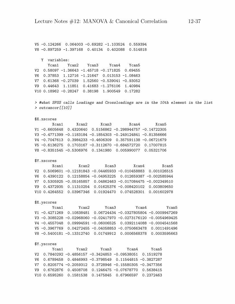
Appendix 2: R: Multivariate Analyses

There is a built-in command in R called cancor(). Using the self-esteem data, we replicatethe output presented earlier in the lecture notes.





> names(data) <- c(paste("v",1:10,sep=""), "sex")

> set1 <- data[,c(1,3,4,5,8)]

> set2 <- data[,c(2,6,7,9,10)]

> outcancor <- cancor(set1,set2)

> summary(outcancor)

Canonical correlation analysis of:

5 X variables: V1, V3, V4, V5, V8

with 5 Y variables: V2, V6, V7, V9, V10

CanR CanRSQ Eigen percent cum scree

1 0.646609 4.181e-01 7.185e-01 88.1417 88.14 ******************************

2 0.250854 6.293e-02 6.715e-02 8.2378 96.38 ***

3 0.130398 1.700e-02 1.730e-02 2.1219 98.50 *

4 0.109654 1.202e-02 1.217e-02 1.4930 99.99 *

5 0.006757 4.565e-05 4.565e-05 0.0056 100.00

Test of H0: The canonical correlations in the

current row and all that follow are zero

CanR LR test stat approx F numDF denDF Pr(> F)

1 0.64661 0.52954 6.7232 25 900.49 <2e-16 ***

2 0.25085 0.91002 1.4556 16 743.01 0.1099

3 0.13040 0.97113 0.7992 9 593.98 0.6172

4 0.10965 0.98793 0.7460 4 490.00 0.5610

5 0.00676 0.99995 0.0112 1 246.00 0.9157

---

Signif. codes: 0 ‘***’ 0.001 ‘**’ 0.01 ‘*’ 0.05 ‘.’ 0.1 ‘ ’ 1

Raw canonical coefficients

X variables:

Xcan1 Xcan2 Xcan3 Xcan4 Xcan5

V1 -0.295453 0.711930 1.03774 -0.066286 -0.146488

V3 0.034786 -0.309300 -0.35480 -0.345545 -1.604935

V4 -0.452470 0.582457 -0.57249 0.825306 0.058419


V5 -0.124266 0.064003 -0.69282 -1.103524 0.559394

V8 -0.897259 -1.397168 0.40134 0.402088 0.514818

Y variables:

Ycan1 Ycan2 Ycan3 Ycan4 Ycan5

V2 0.58097 -1.36643 -1.45718 -0.171825 0.69455

V6 0.37853 1.12716 -1.21647 0.013153 -1.08463

V7 0.61368 -0.27039 1.52560 -0.539041 -0.93052

V9 0.44643 1.11851 0.41683 -1.276106 1.40984

V10 0.18962 -0.28247 0.38198 1.900549 0.17282

> #what SPSS calls Loadings and Crossloadings are in the 10th element in the list

> outcancor[[10]]

$X.xscores


V1 -0.6605648 0.4320640 0.5156862 -0.298944757 -0.14722305

V3 -0.4771399 -0.1183184 -0.1854303 -0.249124841 -0.81356666

V4 -0.7047613 0.3984233 -0.4606309 0.357591138 -0.06721679

V5 -0.6136275 0.1703167 -0.3112670 -0.684572720 0.17007815

V8 -0.8351545 -0.5306976 0.1341980 0.005990077 0.05321706

$Y.xscores


V2 0.5069601 -0.12181843 -0.04465933 -0.010458883 0.001026515

V6 0.4390122 0.12158854 -0.04953225 0.012659387 -0.002585944

V7 0.5305925 -0.05165857 0.04862463 -0.017084475 -0.002349510

V9 0.4372935 0.11310254 0.01625376 -0.008420102 0.003809650

V10 0.4264552 0.03967346 0.01924470 0.074528301 0.001602978

$X.yscores


V1 -0.4271269 0.10838481 0.06724434 -0.0327805804 -0.0009947269

V3 -0.3085228 -0.02968060 -0.02417970 -0.0273176120 -0.0054969425

V4 -0.4557048 0.09994591 -0.06006525 0.0392114088 -0.0004541568

V5 -0.3967769 0.04272455 -0.04058853 -0.0750663478 0.0011491496

V8 -0.5400181 -0.13312740 0.01749912 0.0006568378 0.0003595663

$Y.yscores


V2 0.7840292 -0.4856157 -0.3424853 -0.09538051 0.1519278

V6 0.6789458 0.4846993 -0.3798549 0.11544815 -0.3827287

V7 0.8205774 -0.2059312 0.3728946 -0.15580305 -0.3477356

V9 0.6762876 0.4508708 0.1246475 -0.07678770 0.5638415

V10 0.6595260 0.1581538 0.1475845 0.67966597 0.2372463


The package CCA also performs canonical correlation in R and provides some additionalplots. This website shows some exampleshttp://www.ats.ucla.edu/stat/r/dae/canonical.htm

Another useful package is the candisc package. Check out the commands candisc() andcandiscList() for examples on how to run multivariate linear regressions, which means thaton the DV side there are multiple variables and on the predictor side there is an ANOVA orregression style set of predictors depending whether the predictors are categorical, continu-ous or both). The help page for candisc() gives details. For example, after running candiscand saving the object in R to, say, out.can, the correlations between each variable and thecanonical function is give by out.can[[14]] or out.can$structure and the canonical scores foreach subject on each canonical variable appear in out.can[[15]] or out.can$scores. To get thenames of the attributes of the out.can object just use the names() or attributes() command.The weights to create the new scores are given in out.can[[12]] or out.can$coeffs.raw. Tofind out a list of all relevant output type attributes(out.can) and you’ll see where I got theinformation. For example,

> library(candisc)





> colnames(data) <- c(paste("v",1:10,sep=""), "sex")

> #run manova with grouping code

> out.manova <- manova(data[,1:10] ~ factor(data[,11]))

> summary(out.manova)

Df Pillai approx F num Df den Df Pr(>F)

factor(data[, 11]) 1 0.024698 0.61029 10 241 0.8045

Residuals 250

> #get discriminant weights

> out.can <- candisc(out.manova)

> summary(out.can)

Canonical Discriminant Analysis for factor(data[, 11]):

CanRsq Eigenvalue Difference Percent Cumulative

1 0.024698 0.025323 100 100

Class means:

[1] -0.12644 0.19869

std coefficients:

http://www.ats.ucla.edu/stat/r/dae/canonical.htm


v1 v2 v3 v4 v5 v6 v7 v8

0.458113 0.264415 0.553341 0.028424 -0.762858 -0.105807 0.208394 0.403067

v9 v10

-0.290747 0.482753

> out.can$structure

Can1

v1 0.22094741

v2 0.18563018

v3 0.47289827

v4 -0.02869638

v5 -0.36913728

v6 -0.05819835

v7 0.18597150

v8 0.31324041

v9 -0.09088044

v10 0.24998353

> #out.can[[14]] this line is equivalent to previous line

> out.can$coeffs.raw

Can1

v1 0.49375240

v2 0.45936937

v3 0.81824584

v4 0.03137036

v5 -0.87959886

v6 -0.17762553

v7 0.31952943

v8 0.63412815

v9 -0.50816159

v10 0.70853908

> attributes(out.can)

$names

[1] "dfh" "dfe" "eigenvalues" "canrsq" "pct"

[6] "rank" "ndim" "means" "factors" "term"

[11] "terms" "coeffs.raw" "coeffs.std" "structure" "scores"

$class

[1] "candisc"


> #plot, see help file for details

> plot(out.can)

●

●

1 2

−4

−3

−2

−1

01

23

Canonical scores

factor(data[, 11])

Can

1 (1

00%

)

Structure

v1

v2

v3

v4

v5

v6

v7

v8

v9

v1

0

The built-in command manova() performs multivariate tests like the Pillai, Roy and Wilkstests. The command has the matrix of dependent variables on the left hand side of the tildeand the predictors/grouping codes on the right hand side. See the self-esteem code abovethat has 10 columns of data on the dependent variable side (i.e., data matrix columns 1 to10) and one grouping code (column 11 of data matrix).

Some interesting plots from the output of manova.

> #heplot (hypothesis and error ellipsoid plot);

> #see package help

> library(heplots)

> heplot(out.manova,fill=T)


0.0 0.5 1.0 1.5 2.0 2.5

1.5

2.0

2.5

3.0

v1

v2 +

Error

factor(data[, 11])

●●

12

Documents

Lecture Notes #12: MANOVA & Canonical Correlation 12-1gonzo/coursenotes/file12.pdf · I will now use our new knowledge of matrix manipulations to show how a simple formulation can