Embed Size (px)
Citation preview

Lecture Notes for Statistical Mechanics
Fall 2010
Lecturer: Professor Malvin RudermanTranscriber: Alexander Chen
December 15, 2010
Contents
1 Lecture 1 31.1 Basic Information . . . . . . . . . . . . . . . . . . . . . . . . . . . . . . . . . . . . . . . . . . 31.2 Fundamental Assumption of Statistical Mechanics . . . . . . . . . . . . . . . . . . . . . . . 31.3 Energy and Expectation Values . . . . . . . . . . . . . . . . . . . . . . . . . . . . . . . . . . 31.4 Justification of the Assumption that P Only Depends on E . . . . . . . . . . . . . . . . . . 41.5 Deriving the Fundamental Theorem . . . . . . . . . . . . . . . . . . . . . . . . . . . . . . . 41.6 An Example . . . . . . . . . . . . . . . . . . . . . . . . . . . . . . . . . . . . . . . . . . . . . 5
2 Lecture 2 62.1 Some Remarks . . . . . . . . . . . . . . . . . . . . . . . . . . . . . . . . . . . . . . . . . . . 62.2 Harmonic Oscillator Example, Continued . . . . . . . . . . . . . . . . . . . . . . . . . . . . 62.3 Some Note about Counting . . . . . . . . . . . . . . . . . . . . . . . . . . . . . . . . . . . . 7
3 Lecture 3 9
4 Lecture 4 124.1 A Homework Problem . . . . . . . . . . . . . . . . . . . . . . . . . . . . . . . . . . . . . . . 124.2 About the definiton of Entropy . . . . . . . . . . . . . . . . . . . . . . . . . . . . . . . . . . 124.3 About Thermodynamics . . . . . . . . . . . . . . . . . . . . . . . . . . . . . . . . . . . . . . 13
5 Lecture 5 145.1 Some Statements on Entropy . . . . . . . . . . . . . . . . . . . . . . . . . . . . . . . . . . . 145.2 The Chemical Potential . . . . . . . . . . . . . . . . . . . . . . . . . . . . . . . . . . . . . . 14
6 Lecture 6 156.1 Review . . . . . . . . . . . . . . . . . . . . . . . . . . . . . . . . . . . . . . . . . . . . . . . . 156.2 Reactions . . . . . . . . . . . . . . . . . . . . . . . . . . . . . . . . . . . . . . . . . . . . . . 15
7 Lecture 7 187.1 The Entropy of Mixing . . . . . . . . . . . . . . . . . . . . . . . . . . . . . . . . . . . . . . . 187.2 The Chemical Potential for Photons . . . . . . . . . . . . . . . . . . . . . . . . . . . . . . . 19
1
8 Lecture 8 21
9 Lecture 9 22
10 Lecture 10 2410.1 Digestion on Distributions . . . . . . . . . . . . . . . . . . . . . . . . . . . . . . . . . . . . . 2410.2 Historical Notes . . . . . . . . . . . . . . . . . . . . . . . . . . . . . . . . . . . . . . . . . . . 25
11 Lecture 11 2611.1 Classical Systems . . . . . . . . . . . . . . . . . . . . . . . . . . . . . . . . . . . . . . . . . . 26
12 Lecture 12 2812.1 Canonical Ensemble . . . . . . . . . . . . . . . . . . . . . . . . . . . . . . . . . . . . . . . . 29
13 Lecture 13 3013.1 Continue on Canonical Ensembles . . . . . . . . . . . . . . . . . . . . . . . . . . . . . . . . 3013.2 Grand Canonical Ensemble . . . . . . . . . . . . . . . . . . . . . . . . . . . . . . . . . . . . 31
14 Lecture 14 33
15 Lecture 15 34
16 Lecture 16 37
17 Lecture 17 4017.1 Problem of White Dwarf Star . . . . . . . . . . . . . . . . . . . . . . . . . . . . . . . . . . . 4017.2 Heavy Atoms . . . . . . . . . . . . . . . . . . . . . . . . . . . . . . . . . . . . . . . . . . . . 41
18 Lecture 18 4318.1 Paramagnetism . . . . . . . . . . . . . . . . . . . . . . . . . . . . . . . . . . . . . . . . . . . 4318.2 Diamagnetism . . . . . . . . . . . . . . . . . . . . . . . . . . . . . . . . . . . . . . . . . . . . 44
19 Lecture 18 45
20 Lecture 20 4720.1 Superfluids . . . . . . . . . . . . . . . . . . . . . . . . . . . . . . . . . . . . . . . . . . . . . 47
21 Lecture 21 49
22 Lecture 22 52
2

Statistical Mechanics Lecture 1
1 Lecture 1
1.1 Basic Information
Course Instructor: Malvin RudermanOffice Hour: Tue 1:10 - 2:00 pm, Wed 12:00 - 1:30 pmTextbook: Statistical Mechanics by Pathria
1.2 Fundamental Assumption of Statistical Mechanics
If we take a system of N particles in a container of volume V , in order to know the basic properties of thesystem, we need to construct a general Hamiltonian of N coordinates and N momentum of these particles,and solve for its eigenvalues, which are the energy levels achievable by this system. In general this willbe a very difficult problem, as the Hamiltonian will usually involve complicated interactions between theparticles and it will become a messy manybody problem.
But we don’t do that in statistical mechanics. What we do is to assume that the energy eigenvalues areknown, and we want to know the behavior of the system in finite temperature. Take a system of N particlesin a heat bath of temperature T , wait until equilibrium, then we measure the energy of the system. Notethat by wait until equilibrium we mean that we wait until every state is accessible, after sufficiently longtime. The fundamental theorem of statistical mechanics states that the probability of finding the systemin a state with energy Ei is:
Pi =e−Ei/kBT∑
all states e−Ei/kBT
(1.1)
The quantity in the denominator is called the Partition Function and is usually denoted by Q (not Z?).This theorem tells us that the probability is only dependent on the energy of that state, and that the statewith lowest energy, i.e. the ground state, is the most probable state.
1.3 Energy and Expectation Values
Now that we know the probability of states, we can calculate the average energy of the system, and theexpectation of other observables, too. The average energy, by definition, is just
〈E〉 =∑i
PiEi (1.2)
However, the expectation of the square of the energy,⟨E2⟩
=∑PiE
2i is not, in general, equal to the
square of the average energy. So there usually exists fluctuations:⟨(∆E)2
⟩=⟨E2⟩− 〈E〉 > 0 (1.3)
In general we can estimate the magnitude of the fluctuation:⟨(∆E2)
⟩〈E〉2
∼ O(1
N) (1.4)
so the fluctuation is negligible for a large enough system. In such a system, we can talk about “the energy”of the system, but in smaller systems we need to distinguish between the expectation value of energy, themedian value of energy, or the most probable energy.
3
Statistical Mechanics Lecture 1
The expectation value of any observable can be calculated in the same way, i.e.
〈A〉 =∑i
Pi 〈i|A|i〉 (1.5)
1.4 Justification of the Assumption that P Only Depends on E
Let us consider a 2-state problem where states φ1 and φ2 have the same energy. This can be due to physicalseparation by a potential barrier. Now we can form symmetric and antisymmetric linear combinations ofthese states which will be the ground state and the excited state. No matter what is the initial state, thetime evolution of that state will look like the following:
|φ(t)〉 = cosωt |φ1〉+ sinωt |φ2〉 (1.6)
The state just oscillates between the two states. So if we do a time average, the probability of findingthe particle in either state is 1/2.
We can consider a particle with n states using Fermi’s Golden Rule:
1
τi→j=
2π
~|V 2ij |dnidE
(1.7)
If a particle is in state i and can decay into some states j, and particle in states j can also jump back,then we can calculate the probability change of the particle to be found in state i:
dPidt
= −∑j
| 〈j|V |i〉 |2Pi +∑j
| 〈i|V |j〉 |2Pj =∑j
| 〈i|V |j〉 |2(Pj − Pi) (1.8)
so if the system is in equilibrium and probabilities become stable, then the probability of the particle tobe in state i must be the same as in state j.
1.5 Deriving the Fundamental Theorem
Our fundamental assumption is that the probabilities only depend on the temperature and the energy ofthe state Ei. So we can write the probability of finding the system in state i as a function Pi(T,Ei). Nowwe want to study it using some invariance. Because energy scale is usually arbitrary, and we should havethe freedom to choose the reference point of energy without modifying the relative probabilities, we havethe following invariance:
Pi(T,Ei)
Pj(T,Ej)=Pi(T,Ei + α)
Pj(T,Ej + α)(1.9)
This is a functional equation and the only solution is:
Pi =e−Eiβ(T )∑i e−Eiβ(T )
(1.10)
where β(T ) is an (yet) unknown function of T .Now we ask the question whether β(T ) depends on the detail properties of the system we consider.
Suppose we have two systems 1 and 2, and they have β1(T ) and β2(T ) in the probability formula. Nowsuppose they are each in equilibrium at temperature T , and brought together to form a new system 3,
4

Statistical Mechanics Lecture 1
which has β(T ). The probability of system to be in state ij (system 1 is in state i and system 2 in statej) is:
Pij =e−(Ei+Ej)β(T )∑ij e−(Ei+Ej)β(T )
(1.11)
But we can also think of the system as a composite one and the same probability can be expressed asthe product of individual probabilities:
Pij = PiPj =e−Eiβ1(T )∑i e−Eiβ1(T )
e−Ejβ2(T )∑j e−Ejβ2(T )
(1.12)
the two ways of calculation are the same if and only if β(T ) = β1(T ) = β2(T ). So we can conclude that theβ(T ) function is independent of the details of the system. So the only thing we need to do is to determineβ(T ) for one simple system.
Consider one particle in a 1D box (infinite well). We know from elementary quantum mechanics that
En = ~22m
(nπl
)2. Plug this into the above formula for probability and expectation value, we get:
〈E〉 =1
2β(T )(1.13)
Generalizing this calculation into 3D and N particles, we get 〈E〉 = 3N2β(T ) . But we know from the
classical theory of ideal gases, that 〈E〉 = 32NkBT . So we know that:
β(T ) =1
kBT(1.14)
1.6 An Example
Consider the harmonic oscillator potential. We know that the energy level is proportional to n. Let us omitthe zero point energy of 1
2~ω for now and assume that En = n~ω. We can easily calculate the partitionfunction for one particle since it is just a geometric series:
Q =∑i
e− n~ωkBT =
1
1− e−~ω/kBT,
1
Q= 1− e−~ω/kBT (1.15)
So we can see that the probability of finding the particle in state n goes like e−αn. Now suppose wehave more particles. If there are two particle, then the energy becomes E = (n1 + n2)~ω and there isdegeneracy. The number of states corresponding to the same E is proportional to E. Generalizing thisresult, for N particles, the number of states with the same energy is proportional to En−1.
To be continued. . .
5
Statistical Mechanics Lecture 2
2 Lecture 2
2.1 Some Remarks
Recall that last time we argued the form of the fundamental theorem of Statistical Mechanics. Theargument was based on first principles, but there is one assumption which is not first principle, i.e. weassumed that the perturbation of energy is hermitian:
| 〈i|V |j〉 |2 = | 〈j|V |i〉 |2 (2.1)
This assumption may not be true if the transition is not time-reversible.
2.2 Harmonic Oscillator Example, Continued
Consider again the harmonic oscillator example. We want to study how physics change from 1 particle toN particles. We have already known the form of probability of the system taking energy level n for 1 and2 particles, we can anticipate that for N particles it is:
N = 1 : Pn =e−n~ω/kT
Q=(
1− e−~ω/kT)e−n~ω/kT
N = 2 : Pn =ne−n~ω/kT
Q. . . . . .
N = N : Pn ∼nN−1e−n~ω/kT
Q
the Q is there to ensure proper normalization, so that∑
i Pn = 1. We will show that the final line is trueusing some approximations.
Because the energy level of the whole N particle system is just the sum of energy levels of individualparticles, we have:
n = n1 + n2 + · · ·+ nN (2.2)
E = E1 + E2 + · · ·+ EN (2.3)
In the case where kT is much greater than ~ω, we can think of the energy levels being continuous,because the little steps of energy will not introduce much error in our approximation. Therefore wecan replace summation by integrals and the result will look much nicer. In order to calculate the totalprobability, we basically integrate over all the possible configurations:
P (n) =
∫ ∫. . .
∫P (n− n1 − n2 − · · · − nN−1)P1(n1)P2(n2) . . . dn1dn2 . . . dnN−1 (2.4)
This integral looks quite difficult, but we can do it in Fourier space. After Fourier transform, we have:∫ ∞−∞
eiknP (n)dn =
[∫ ∞−∞
eikn1P1(n1)dn1
]N(2.5)
We can take the P1(n) = 0 for all n < 0 and do the integral on P1:
6

Statistical Mechanics Lecture 2
P1(k) =
∫ ∞0
eikn−~ωβndn =1
ik − ~ωβ(2.6)
And doing a Fourier transform back, we can find
P (n) =1
2π
∫ ∞−∞
e−ikn(Pi(k)
)dk (2.7)
Because P1(k) ≤ 1, the N power will damp everywhere except for the highest point, which will turn tosomewhat like a gaussian. Therefore the P (n) should also resemble a gaussian in the large N limit. Nowlet’s evaluate the above integral analytically. We substitute z = k − (−iβ~ω) and convert the integral toa contour integral:
P (n) = e−n~ωβ∮
dz
zNeinz (2.8)
where we close the countour from below, because z has a pole in the lower halfplane. In the end we have
PN (E) =eβEEN−1
(N − 1)!. The most probable energy can be found by solving the equation ∂
∂EPN (E) = 0, and
the result is:
E = (N − 1)kT (2.9)
We can also find the width of this near-gaussian distribution, by looking at the two points where thesecond derivatives change sign. These can be found by solving ∂2
∂E2PN (E) = 0 and the answer is:
δE = ± 2
β(N − 1)1/2 (2.10)
2.3 Some Note about Counting
Consider N particles in a volume V . We have a smaller volume v inside V and we want to ask questionslike “what is the probability of finding n particles inside the volume v?”.
First let’s recall the binomial expansion
(p+ q)N =N∑n=0
(N
n
)pnqN−n (2.11)
where the binomial coefficients are defined to be
(N
n
)=
N !
n!(N − n)!. If we let p+ q = 1 then we have
1 =
N∑n=1
N !
n!(N − n)!pn(1− p)N−n (2.12)
for any p < 1. Suppose we are considering classical particles, finding a particle inside a volume v insidea box V is just v/V , and if we substitute p = v/V into the above equation, then the summand is justthe probability of finding n out of N particles inside volume v at any given time. If we consider quantummechanics, then we need to integrate the wavefunction square, but just need to replace p.
Consider some extremes. For n = N , i.e. all the particles squeezed inside v, the probability is:
7
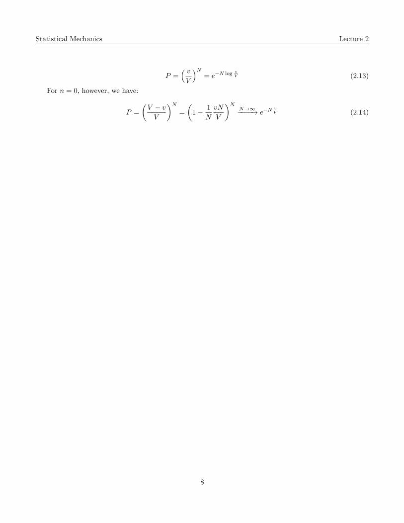
Statistical Mechanics Lecture 2
P =( vV
)N= e−N log v
V (2.13)
For n = 0, however, we have:
P =
(V − vV
)N=
(1− 1
N
vN
V
)NN→∞−−−−→ e−N
vV (2.14)
8

Statistical Mechanics Lecture 3
3 Lecture 3
What we have discussed is how statistical mechanics might have developed if we had the knowledge ofquantum levels and stuff. We started out with a fundamental assumption that all states with the sameenergy are equally probable in equilibrium. The key is that we have a hamiltonian with a little perturbationwhich permits time-reversible transitions.
Recall last time we did some counting exercise, and found that for N particles in volume V , theprobability of finding n particles in smaller volume v is:
P (n) =N !
n!(N − n)!
( vV
)n(V − vV
)N−n(3.1)
We will often use some approximations:
n! =
∫ ∞0
e−xxndx (3.2)
log n! = n log n− n+1
2log n (3.3)
where the latter equation is called the Stirling approximation. Which means that for n! = n(n − 1)(n −2) · · · ∼ nn
en = nne−n. If we take these expressions and use them on the previous expression of P (n) tocalculate logP (n), then we can see the graph is like a thin Gaussian, which peaks at around N/2. Thepeak probability is about 1/
√N , and width is about
√N .
Recall if we want to measure a quantum mechanical variable A, the expectation value we get is
〈A〉 =∑i
Pi 〈i|A|i〉 (3.4)
and usually we have⟨A2⟩6= 〈A〉2. If we go to N →∞ limit, then the system has well-defined energy, but
there are some variables of particular interest. This is called the thermodynamics limit. The thermody-namic variables fall into two categories:
• Extensive variables: U , CV , S, N , these variables increase as the size of the system increases.
• Intensive variables: T , P , these variables do not increase as the size of the system increases.
Now let’s turn to the special variable “entropy”, which is the missing link between thermodynamics andstatistical mechanics. We want to define entropy and find the way to calculate it. Consider two adjacentboxes labeled 1 and 2, they are connected to form system 3. Label the states in 1 by i and states in 2 byj, we have:
P(3)ij = P
(1)i P
(2)j (3.5)
To form an extensive quantity, i.e. S(3) = S(2) + S(1), it is appealing to define S =∑
i logPi, butbecause probability for some high energy states goes to zero, this definition will lead easily to infinities.
What about define S = −k∑
i Pi logPi? We can calculate the entropy of system 3 as:
9
Statistical Mechanics Lecture 3
S(3) = −k∑i
∑j
(PiPj) log(PiPj) = −k∑ij
(PiPj logPi + PiPj logPj) = −k(∑i
Pi logPi +∑j
Pj logPj)
(3.6)this quantity is manifestly extensive and this is what we want. This definition is good even if the systemis not in thermal equilibrium, because whatever is the stucture of Pi, this expression still works.
If we look at distribution of Pi of states with almost exactly same energy, then Pi =1
Niwhere Ni is
the number of that state. The entropy in this case is:
S = −k∑i
Pi logPi = k logNi (3.7)
This definition of entropy is such that when you depart from the thermodynamic equilibrium, theentropy lowers. In other words, the entropy takes maximum at thermodynamic equilibrium. This is howwe interpret entropy physically.
Remember in thermodynamics we defined entropy as a function of P and V and T . When you integratealong the change of the system from A to B:
S =
∫ B
A
dQ
T(3.8)
the integral is independent of path and is defined to be the entropy change. The second law of thermody-namics says this function always exists.
We introduced two potentials in thermodynamics:
1. Helmholtz Free Energy: F = U − ST
2. Gibbs Free Energy: G = U − ST + PV
These quantities are useful in special circumstances when we want to isolate some thermodynamic effect.Say if we study a system with fixed temperature, then the system tends to minimize its Helmholtz freeenergy. If we consider pressure fixed instead of the volume, then we use Gibbs free energy, which also tendsto be minimized.
The name “Entropy” is the greek word for “transformation”. In some sense, it measures how muchtransformation was done on the system. What about “free energy”? Let’s consider the change of Helmholtzfree energy:
dF = dU − TdS − SdT (3.9)
Because we have
1. ∆Q = dU + PdV
2. ∆Q = TdS
so we can rewrite the change of free energy to dF = −PdV −SdT . On an isotherm, then dF = −PdVwhich is the work done to the outside world if we allow the volume to change. In this sense, it is “free”.
Let’s look back at the definition of S. We can plug in the canonical probability distribution:
10

Statistical Mechanics Lecture 3
S = −k∑ e−Ei/kT
Qlog
e−Ei/kT
Q= k
∑PiEikT
+ k logQ∑
Pi =U
T+ k logQ (3.10)
Compare the expression with the definition of the Helmholtz energy, we see that:
F = −kT logQ, Q = e−F/kT (3.11)
which relates the Helmholtz free energy directly to the partition function.Let’s consider an example. Combining the first and second law of thermodynamics, we have TdS =
dU + PdV , so we know that:
dS =dU
T+P
TdV =
1
T
(∂U
∂V
)T
dV +1
T
(∂U
∂T
)V
dT +P
TdV (3.12)
=
(∂S
∂T
)V
dT +
(∂S
∂V
)T
dV (3.13)
Equating corresponding terms, and using the Maxwell relation
(∂S
∂V
)T
=
(∂P
∂T
)V
, we get P =
−(∂U
∂V
)T
+ T
(∂P
∂T
)V
.
In microscopic view, we can calculate the pressure by calculating the expectation of energy changewhen changing volume:
P =∑i
(∂Ei∂V
)e−Ei/kT
Q(3.14)
which is much harder.
11
Statistical Mechanics Lecture 4
4 Lecture 4
4.1 A Homework Problem
Remember in our Hilbert space the basis we use is the energy eigenbasis H |i〉 = Ei |i〉. So the expectationvalue of variable A is just 〈A〉 =
∑Pi〈i|A|i〉. Now what if we change into the eigenbasis of operator A, i.e.
A |j〉 = Aj |j〉, then is the following expression equivalent to our previous expectation value?∑Aje
−〈j|H|j〉β(T ) = 〈A〉 (4.1)
4.2 About the definiton of Entropy
There are two points about the entropy we introduced by the formula S = −k∑Pi logPi:
• It is the same entropy as we introduced in thermodynamics.
• It is still a good definition even when not in equilibrium.
The second point is easier to see because the definition is robust, as it only uses the concept of probability.In order to see the first point, let’s calculate the change in entropy:
∆S = −k∑i
∆(Pi logPi) = −k∑i
(∆Pi logPi −∆Pi) (4.2)
And by the fundamental theorem, we have logPi = −βEi − logQ, we now have:
∆S = kβ∑i
(∆Pi)Ei + k∑i
∆Pi logQ = kβ∑i
(∆Pi)Ei
= kβ∑i
∆(PiEi)− kβ∑i
Pi∆Ei(4.3)
The first term is just ∆U , where U = 〈E〉. The second term can be interpreted by noting thatdEi = ∂Ei/∂V dV , which is just −PdV . Therefore we have:
T∆S = ∆U + P∆V (4.4)
which is just the statistical mechanics version of the second law of thermodynamics.We saw that in a system with N states of equal energy, the probability of finding the system in any
state is the same: Pi = 1/N . This can be accomplished by introducing a small perturbation which allowsreversible transition between different states. If we adopt the above definition of entropy, we can calculatethe entropy of the system:
S = −k〈logP 〉 = −k∑i
1
Nlog
1
N= k logN (4.5)
The same definition leads to the fact that at zero temperature, all states have probability of unity, sothe entropy is zero. This is the third law of thermodynamics.
12
Statistical Mechanics Lecture 4
4.3 About Thermodynamics
Remember our introduction of thermodynamic potentials. In addition to what we have introduced, wewant to study situations where the number of particles can vary, like that in a chemical reaction. Similarproblems include e−+e+ −→ γ where we are interested in the equilibrium temperature and absolute valueof entropy.
Remember last time we derived the expression of pressure:
P = −(∂U
∂V
)T
+ T
(∂P
∂T
)V
(4.6)
this was done by using the thermodynamic identities, which was much easier than using first principlesfrom statistical mechanics. When there is a large number of particles, we can do things easier by usingthermodynamics.
Remember we introduced the Helmholtz free energy F = U − ST , which satisfies an elegant relationF = −kT logQ. And the change in free energy is:
dF = dU − TdS − SdT = −PdV − SdT (4.7)
By the way of taking differentials, we know that P = −(∂U
∂V
)T
and S = −(∂U
∂T
)V
. Now suppose
we change the number of particles in the system, we introduce the change in the free energy by:
dF = −PdV − SdT + µdN (4.8)
where N is the number of particles and µ can be identified as µ =
(∂F
∂N
)V,T
. It is similar to a binding
energy, but in a more general form. Now if we look at the system energy instead, we add the same term
to the change of internal energy, and we get another expression of µ as µ =
(∂U
∂N
)V,S
. Now what if we
consider the Gibbs free energy?
dG = dU − SdT − TdS + PdV + V dP + µdN = −SdT + V dP + µdN (4.9)
Consider if we fix the temperature and pressure of the system, and we remove one particle, the systemadjusts its volume automatically to accomodate the change, and the other particles do not feel the change.Another way to say this is that both P and T are intensive quantities, so they don’t depend on the particlenumber. Therefore (
dG
dN
)P,T
= µ(P, T ), G = µ(P, T )N (4.10)
Next time we will consider things like vapor pressure and osmotic pressure.
13
Statistical Mechanics Lecture 5
5 Lecture 5
5.1 Some Statements on Entropy
Remember we defined the entropy in the statistical mechanics sense:
S = −k∑
Pi logPi (5.1)
and we derived some properties such as −kT logQ = U −TS = F . If we are looking at an isolated system,it tends to maximize its entropy.
If we are looking S and treat it classically, then it is always infinity. In classical situation, the distancebetween states is going to zero, and instead of discrete states we get a contiuum of states. So all theentropies go to infinity. However, sometimes knowing the value of S will be helpful in some situationswhen we want to ask all kinds of questions about the system.
The second statement about entropy is that when temperature goes to zero, S goes to 0. This hasthe implication that all specific heat should approach zero at zero temperature. In order to see this, let’ssuppose that S = κTα where α is a positive number. We have
dS
dT= καTα−1 =
1
T
DQ
dT=
1
TCV =⇒ CV ∝ Tα (5.2)
5.2 The Chemical Potential
Remember that we derived the various expressions for the chemical potential
µ =
(∂F
∂N
)T,V
=
(∂G
∂N
)P,T
=
(∂U
∂N
)S,V
= −T(∂S
∂N
)U,V
(5.3)
And we also know that G = Nµ(P, T ). The change in chemical potential is
dµ =dG
N= − S
NdT − V
NdP (5.4)
14

Statistical Mechanics Lecture 6
6 Lecture 6
6.1 Review
Remember we introduced the fundamental assumption of statistical mechanics, and defined the entropy as
S = −〈k logPi〉 = −k∑i
Pi logPi (6.1)
and we have the relation between the Helmholtz free energy and partition function
F = U − ST = −kT logQ (6.2)
From the definition of Helmholtz free energy we have some relations
S = −(∂F
∂T
)N,V
(6.3)
P = −(∂F
∂V
)N,T
(6.4)
U = 〈E〉 = −∂ logQ
∂β(6.5)
and we have several expressions for chemical potential
µ =
(∂F
∂N
)T,V
=
(∂G
∂N
)P,T
=
(∂U
∂N
)S,V
= −T(∂S
∂N
)U,V
(6.6)
In order to find the absolute value of µ, the easiest way is to fix temperature and volume and calculatethe Helmholtz free energy of the system, then differentiate it with respect to particle number N and weget µ. We are going to do this in a moment.
6.2 Reactions
Consider a chemical (or particle) reaction
A+B ←→ C (6.7)
When equilibrium is achieved, the Gibbs free energy is at its minimum, and the particle numbers of differentspecies should be equal, so the chemical potentials should satisfy
µA + µB − µC = 0 (6.8)
But does the method that we achieve equilibrium matter? What if we release a photon during thischemical process? Do we need to calculate the chemical potential for photons? We will address thesequestions in this lecture. We will consider processes like e− + e+ −→ γ + γ and H+ + e− −→ H which areelementary processes of the universe.
Consider a 1 dimensional harmonic oscillator, we know the energy levels to be En = (n + 1/2)~ω0, sowe can calculate the partition function
Q1 =∑n
e−(n+ 12
)~ω0β =e−
12~ω0β
1− e−~ω0β(6.9)
15
Statistical Mechanics Lecture 6
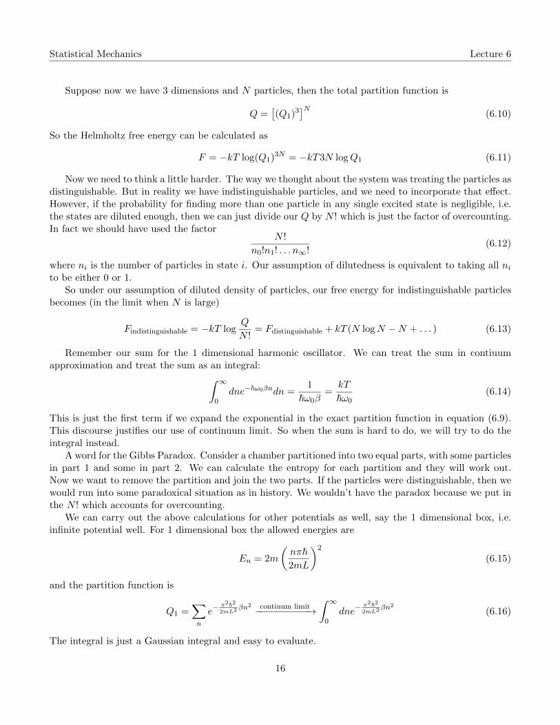
Suppose now we have 3 dimensions and N particles, then the total partition function is
Q =[(Q1)3
]N(6.10)
So the Helmholtz free energy can be calculated as
F = −kT log(Q1)3N = −kT3N logQ1 (6.11)
Now we need to think a little harder. The way we thought about the system was treating the particles asdistinguishable. But in reality we have indistinguishable particles, and we need to incorporate that effect.However, if the probability for finding more than one particle in any single excited state is negligible, i.e.the states are diluted enough, then we can just divide our Q by N ! which is just the factor of overcounting.In fact we should have used the factor
N !
n0!n1! . . . n∞!(6.12)
where ni is the number of particles in state i. Our assumption of dilutedness is equivalent to taking all nito be either 0 or 1.
So under our assumption of diluted density of particles, our free energy for indistinguishable particlesbecomes (in the limit when N is large)
Findistinguishable = −kT logQ
N != Fdistinguishable + kT (N logN −N + . . . ) (6.13)
Remember our sum for the 1 dimensional harmonic oscillator. We can treat the sum in contiuumapproximation and treat the sum as an integral:∫ ∞
0dne−~ω0βndn =
1
~ω0β=
kT
~ω0(6.14)
This is just the first term if we expand the exponential in the exact partition function in equation (6.9).This discourse justifies our use of continuum limit. So when the sum is hard to do, we will try to do theintegral instead.
A word for the Gibbs Paradox. Consider a chamber partitioned into two equal parts, with some particlesin part 1 and some in part 2. We can calculate the entropy for each partition and they will work out.Now we want to remove the partition and join the two parts. If the particles were distinguishable, then wewould run into some paradoxical situation as in history. We wouldn’t have the paradox because we put inthe N ! which accounts for overcounting.
We can carry out the above calculations for other potentials as well, say the 1 dimensional box, i.e.infinite potential well. For 1 dimensional box the allowed energies are
En = 2m
(nπ~2mL
)2
(6.15)
and the partition function is
Q1 =∑n
e−π2~22mL2 βn
2 contiuum limit−−−−−−−−−−→∫ ∞
0dne−
π2~22mL2 βn
2
(6.16)
The integral is just a Gaussian integral and easy to evaluate.
16
Statistical Mechanics Lecture 6
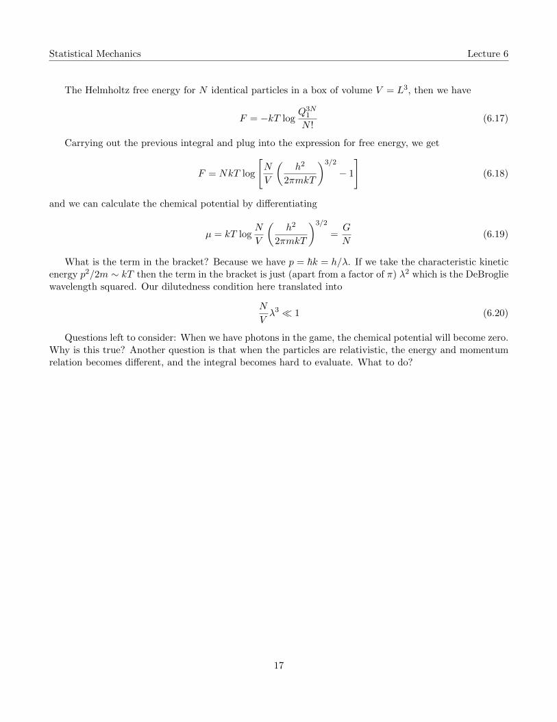
The Helmholtz free energy for N identical particles in a box of volume V = L3, then we have
F = −kT logQ3N
1
N !(6.17)
Carrying out the previous integral and plug into the expression for free energy, we get
F = NkT log
[N
V
(h2
2πmkT
)3/2
− 1
](6.18)
and we can calculate the chemical potential by differentiating
µ = kT logN
V
(h2
2πmkT
)3/2
=G
N(6.19)
What is the term in the bracket? Because we have p = ~k = h/λ. If we take the characteristic kineticenergy p2/2m ∼ kT then the term in the bracket is just (apart from a factor of π) λ2 which is the DeBrogliewavelength squared. Our dilutedness condition here translated into
N
Vλ3 1 (6.20)
Questions left to consider: When we have photons in the game, the chemical potential will become zero.Why is this true? Another question is that when the particles are relativistic, the energy and momentumrelation becomes different, and the integral becomes hard to evaluate. What to do?
17

Statistical Mechanics Lecture 7
7 Lecture 7
Remember last time we studied the N particle partition function when they are indistinguishable
Q =∑
e−Ei/kT = (Q1)N (7.1)
And the free energy is proportional to
F ∝ −kT log
(V
λ3
)N(7.2)
Now if we have identical particles, i.e. indistinguishable. If we continue to use the above expressionthen we are overcounting the states. Remember the approximation we used last time we to assume thatstates are sufficiently diluted and the occupation of any state is no more than 1. Under this approximation
Q =(Q1)N
N !(7.3)
therefore the Helmholtz free energy becomes
F ∝ −kT log
[(N
λ3
N) 1
N !
]≈ −kTN log
V
Nλ3(7.4)
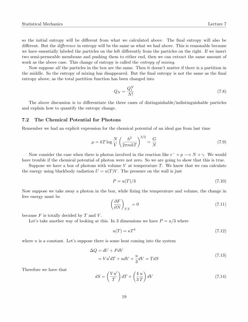
7.1 The Entropy of Mixing
Consider a box of volume V being partitioned into two equal halves, both with volume V/2. Particlesare distributed equally inside two partitions. We know the entropy of the whole system is the sum of theentropies for the two partitions:
S = S1 + S2 = 2
[−kN
2log
(V
2(N/2)λ3
)]+N log
(N
2
)(7.5)
Now if we remove the lid in between, then the entropy of the whole system becomes
S = −kN log
(V
Nλ3
)+N logN (7.6)
and the entropy has increased by ∆S = kN log 2. This is a reversible process. This means that, if we haddone this process carefully, we can extract some work from it, like the Carnot engine. Indeed we can dothis by imagining that we insert a semi-permeable membrane in between which only blocks one specificparticle from going through. When we move the membrane to one end of the box, the system is doing workby this particular particle. Imagine if we have a huge number of this kind of membrane, we can extractwork from every particle in this box, and this is the work we could have extracted from the system. Theamount of energy is gained from the heat absorbed from the reservoir which is kept at constant T .
Now suppose the particles inside this box are indistinguishable. In the case of partitioned box the totalpartition function is
QN =QN1
(N/2)!(N/2)!(7.7)
18
Statistical Mechanics Lecture 7
so the initial entropy will be different from what we calculated above. The final entropy will also bedifferent. But the difference in entropy will be the same as what we had above. This is reasonable becausewe have essentially labeled the particles on the left differently from the particles on the right. If we inserttwo semi-permeable membrane and pushing them to either end, then we can extract the same amount ofwork as the above case. This change of entropy is called the entropy of mixing.
Now suppose all the particles in the box are the same. Then it doesn’t matter if there is a partition inthe middle. So the entropy of mixing has disappeared. But the final entropy is not the same as the finalentropy above, as the total partition function has been changed into
QN =QN1N !
(7.8)
The above discussion is to differentiate the three cases of distinguishable/indistinguishable particlesand explain how to quantify the entropy change.
7.2 The Chemical Potential for Photons
Remember we had an explicit expression for the chemical potential of an ideal gas from last time
µ = kT logN
V
(h2
2πmkT
)3/2
=G
N(7.9)
Now consider the case when there is photon involved in the reaction like e− + p −→ N + γ. We wouldhave trouble if the chemical potential of photon were not zero. So we are going to show that this is true.
Suppose we have a box of photons with volume V at temperature T . We know that we can calculatethe energy using blackbody radiation U = u(T )V . The pressure on the wall is just
P = u(T )/3 (7.10)
Now suppose we take away a photon in the box, while fixing the temperature and volume, the change infree energy must be (
∂F
∂N
)T,V
= 0 (7.11)
because F is totally decided by T and V .Let’s take another way of looking at this. In 3 dimensions we have P = u/3 where
u(T ) = κT 4 (7.12)
where κ is a constant. Let’s suppose there is some heat coming into the system
∆Q = dU + PdV
= V u′dT + udV +u
3dV = TdS
(7.13)
Therefore we have that
dS =
(V u′
T
)dT +
(4
3
u
T
)dV (7.14)
19
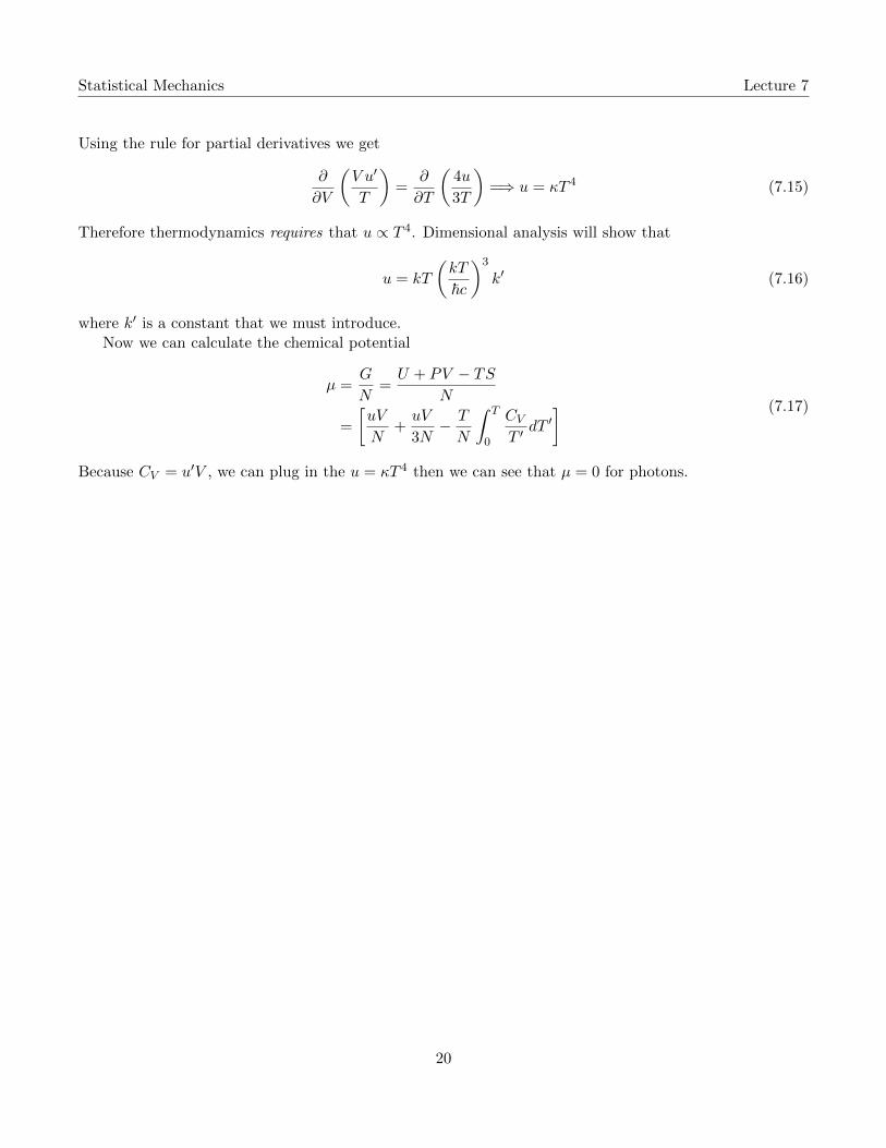
Statistical Mechanics Lecture 7
Using the rule for partial derivatives we get
∂
∂V
(V u′
T
)=
∂
∂T
(4u
3T
)=⇒ u = κT 4 (7.15)
Therefore thermodynamics requires that u ∝ T 4. Dimensional analysis will show that
u = kT
(kT
~c
)3
k′ (7.16)
where k′ is a constant that we must introduce.Now we can calculate the chemical potential
µ =G
N=U + PV − TS
N
=
[uV
N+uV
3N− T
N
∫ T
0
CVT ′dT ′] (7.17)
Because CV = u′V , we can plug in the u = κT 4 then we can see that µ = 0 for photons.
20
Statistical Mechanics Lecture 8
8 Lecture 8
Consider a box of fixed volume V kept at fixed temperature T . The system insided tends to minimize itsHelmholtz free energy F . Remember
dF = dU − TdS − SdT +∑i
µidNi = −SdT − PdV +∑i
µidNi (8.1)
where the sum is over all species of particles inside the box. If we fix T and V , then at equilibrium dF = 0,we have ∑
i
µidNi = 0 for all allowed changes dNi (8.2)
Consider we have a chemical reaction involving particles Ai with number coefficients νi, then we writeour reaction as
∑i νiAi = 0. For example, we can consider H2 + Cl2 ↔ 2HCl. Then νH2 = 1, νCl2 = 1 and
νHCl = −2. In this scenario, then we have ∑i
νiµi = 0 (8.3)
We want to make an assumption that the existence of other kinds of particles will not affect the chemicalpotential of any one species of particles, in the limit of dilute gas. This makes sense because here interactionis not so strong, so that the sum of entropies of two species of particles in two boxes of V is the same asthe entropy if the two species of particles in the same box. Any particle is not aware of the presence ofother species of particles.
Remember for photons µ = 0. For non-relativistic particles we have
µi = kT log
(Niλ
3i
V
)+mic
2 (8.4)
Note because of different energies in binding, we have different mass for, e.g. HCl and H + Cl. That is whywe include the mic
2 term. If we plug the above equation into equation (8.3) then we can get∑i
[kT log
(niλ
3i
)+mic
2]νi = 0 (8.5)
[n1λ31][n2λ
32]
[n3λ33]
= e−∆E/kT (8.6)
where ni is the density of state of state in V . Remember this is non-relativistic.Consider now the process e− + e+ ←→ γ + γ. Because there is degeneracy associated with spin s, we
replace V −→ V (2s+ 1). We write
µe− = kT logn−λ
3−
2s+ 1+mec
2 (8.7)
µe+ = kT logn+λ
3+
2s+ 1+mec
2 (8.8)
Therefore we can evaluate
n+n− =
(2s+ 1
λ3
)2
e−2mc2β (8.9)
But this equation does not tell us either n− or n+. We have to put in some extra condition such as n+ = n−to get the exact value of either number densities.
21
Statistical Mechanics Lecture 9
9 Lecture 9
Up to now we have been considering problems where many particles share a box, but for each state thereis only zero or one particle at that particular state. We derived the chemical potential
µ = kT log
(N
Vλ3
)+mc2 (9.1)
Here λ is about the effective wavelength of the particle. The assumption of diluteness is equivalent to
N
Vλ3 1 (9.2)
Remember also that we have the relation
µ =∂
∂N(U − TS)
∣∣∣∣T,V
(9.3)
So µ can also be thought of something like the binding energy. We can also write
N =V
λ3eµ/kT (9.4)
Consider the reaction e− + H+ ←→ H. We will assume the system is neutral, so that the number ofelectrons is the same as number of ions. We had the result
[λ3ene][nH+λ3
H+ ]
[λ3HnH ]
= e−εb(H)/kT (9.5)
But because we know that the number density of e is the same as H+, while λH ∼ λH+ , so we have
ne =nHλ3e
e−εb/2kT (9.6)
Because the above process is essentially reversible, the rate of both directions should be the same
nen+|H|2ρHγ = nγnH |H|2ρe+ (9.7)
In principle we can invert this equation to get the same ratio as the above. But in nγ there is a factorof c coming into play, while there is no speed of light in the above equation. So there must be a delicatecancelation among the terms to eliminate the speed of light. We know the form of the product nenH+ onthe left hand is approximately
nenH+ ∼ nHnγe−|εb|/kT (9.8)
Because εb ≈ 13.6 eV, the corresponding temperature for equilibrium is k(105 K) ∼ 10 eV.Suppose we have a box with a magnetic field B(x) pointing down which is a function of position. The
particles inside have spin 1/2. We want to know how the distribution of the spin of the particle. Let’sdefine
µ↑ = µB=0 −mB, µ↓ = µB=0 +mB (9.9)
We know from the fundamental assumption of statistical mechanics that in equilibrium we have
n↑ = n(0)e−mB/kT , n↓ = n(0)e+mB/kT (9.10)
22

Statistical Mechanics Lecture 9
Therefore if we take the sum of these two equations, we have
n↑ + n↓ ∝ emB/kT + e−mB/kT = 2 +mB
kT− mB
kT+
(mB
kT
)2
+ . . . (9.11)
Which means that there is an accumulation of particles at places with larger B field.Consider a system with available energy levels. We denote the number of particles at energy level εr
as nr. We have been dealing with the partition function, which can now be written as the sum of states
Q =∑
all distributions of states
e−∑r nrεr/kT (9.12)
subject to the condition that∑
r nr = N . If we ignore the constraint for now, we can write
Q =∏r
∑nr
e−nrεr/kT =∏r
1
1− e−εr/kT(9.13)
This looks like the Einstein-Bose distribution, so if we calculate the Helmholtz free energy we get
F = −kT logQ = kT∑r
log(
1− e−εr/kT)
(9.14)
Remember this result we have is right for photons. But note that F does not depend on N explicitly,so the partial derivative is zero, which means this applies to particles with µ = 0. So we reached anotherresult where the number of particles can vary freely.
Let’s think about this problem in another way. Remember from the beginning we have thought of µas something resulting from the properties of the system. However, we can treat µ as given a priori, andsee what can we get. Consider a box connected with an reservoir with fixed entropy and infinite numberof particles. The chemical potential of the reservoir is just(
∂F
∂N
)T,V
= µ = −|εb| (9.15)
So in equilibrium the µ of the system is the same as that of the reservoir, and we have a way to control thechemical potential. If we call the energy of the reservoir zero, then the energy of the system is shifted by−µ. We want to calculate the average number of particles in a certain state by summing over the possible“state configurations”
〈nr〉 =
∑nrnre−(εr−µ)nrβ∑
nre−(εr−µ)nrβ
(9.16)
Remember the chemical potential of a system is often negative, so the inclusion of µ effectively raises theenergy and suppressed the probability of every state. We can continue playing this game and find anexpression for the expectation value
〈nr〉 =1
β
∂
∂µlog
∞∑nr=0 fix r
e−(εr−µ)nrβ = −kT ∂
∂µlog(
1− e−(εr−µ)/kT)∝ 1
e(εr−µ)/kT − 1(9.17)
So we have derived the Bose-Einstein distribution from first principles.
23
Statistical Mechanics Lecture 10
10 Lecture 10
10.1 Digestion on Distributions
Remember given a system, if we know the partition function of the system, then we can basically answerany questions about the system. However the partition function may be very hard to calculate. Nowconsider we have a system with N particles and some energy levels, last time we employed a trick tocalculate the expectation of occupation number of each state. We shifted the system energy by −µN byadding a reservoir of fixed chemical potential, but now the number of particles in the system is no longerN , but can be varied. Now let’s see how we can do it physically without using the trick.
The results we get from last time is
〈nr〉 =
∑r e−(εr−µ)nr/kTnr∑
r e−(εr−µ)nr/kT
=1
e(εr−µ)/kT − 1(10.1)
This result applies to bosons. What if we have fermions? Remember we can treat the sum as fixing r andsumming up nr, but in the case of fermions nr = 0 or 1, so
〈nr〉f =
∑r e−(εnr−µ)nr/kTnr∑
nre−(εr−µ)nr/kT
=e−(εr−µ)/kT
1 + e−(εr−µ)/kT=
1
e(εr−µ)/kT + 1(10.2)
This is the Fermi-Dirac distribution.Now we want to hold the number of particles in the box fixed. Then we can use the above formula to
compute the chemical potential. We can define the probability with some chemical potential
P (µ) =e−(Ei−Nµ)/kT∑
all states e−(Ei−Nµ)/kT )
(10.3)
Let’s look at an example. Suppose we have an atmosphere of O2, and some Hemoglobin (proteins thatcan have 1 binding site that can bind to oxygen) with binding energy ε. How does the amount of bindingdepend on the pressure of oxygen? We know the chemical potential of oxygen is
µO2 = kT log nO2λ3 (10.4)
This formula applies to perfect dilute gas of indistinguishable paricles. So we can solve for the numberdensity of O2
nO2 =1
λ3eµ/kT (10.5)
So the chemical potential tells us how dilute the gas is compared to the wavelength of the gas particle.The partition function of binding is simple, as it only has two different configurations
Q = 1 + e−ε/kT eµ/kT (10.6)
So the average number of binding
〈nr〉 =1
e(ε−µ)/kT + 1=
1
eε/kT /nO2λ3 + 1
(10.7)
The physical meaning of this expectation is the average occupation number on one Hemoglobin site, whichis between 0 and 1. When temperature goes to 0, the exponential goes to 0 and there is no problem inbinding. When the density of oxygen is infinite then 1/n goes to 0, and this occupation goes to 1 so thereis no objection to binding either.
24

Statistical Mechanics Lecture 10
10.2 Historical Notes
Suppose we have a hamiltonian H(q1, . . . , q3N , p1, . . . , p3N ) which is a function of 6N variables in thephase space. A point in the phase space specifies the system completely. There is an interesting theoremattributed to Liouville, which says the following. Let us assume the hamiltonian to be independent of time,and suppose we have a large number of systems moving around in the phase space with ρ(q1, . . . , p3N )denoting the number density of different systems in the phase space, and the total number of systems isconserved, then we have the conservation equation
∂ρ
∂t+∇ · (ρv) = 0 =
∂ρ
∂t+ ρ∇ · v + v · ∇ρ (10.8)
The comoving density of systems, which is defined to be the total time derivative of ρ is
dρ
dt=∂ρ
∂t+ (v · ∇)ρ = −ρ∇ · v (10.9)
Remember we have the Hamilton’s equations
qi = +∂H
∂pi, pj = −∂H
∂qj(10.10)
So the above equation for derivative for ρ becomes
dρ
dt= −ρ
∑(∂
∂qiqi +
∂
∂pjpj
)= 0 (10.11)
So wherever we sit, the density of system at my neighborhood remains constant, regardless of the detailsof the dynamics of the system. So there is no way you can use a static hamiltonian to focus a densitydistribution in the phase space. If we want to establish a density distribution which does not change withtime, i.e. ∂ρ/∂t = 0, then the only solution is that dρ/dt = 0 and ρ is a constant.
For a classical system we have the expectation of a physical quantity
〈A〉 =
∫dq1 . . . dp3NA(q1, . . . , p3N )e−H/kT∫
dq1 . . . dp3Ne−H/kT(10.12)
Note that this is purely classical and we don’t need to know the density of states. But there is no way wecan calculate the entropy in this classical way, because we defined it to be
S = −k∑
Pi logPi (10.13)
which assumes the knowledge of probabilities of micro states.
25
Statistical Mechanics Lecture 11
11 Lecture 11
We discussed last time that because what we derived, there is no way to focus a parallel beam to a smallerarea of concentration. That was wrong. Only when the incoming beams are diverging that we can’t use astatic device to focus it to a concentrated parallel beam.
Another way of interpreting the Liouville’s theorem is that the comoving density ρ, which is equal to
ρ =d2n
dpdq(11.1)
is constant wherever we move to in phase space. Suppose the distribution n is constant, then this amountsto the constancy of any volume element dpdq that we are moving. So if we have an incoming parallelbeam, then the volume is zero because there is no p dispersion in the y direction, so it is fine to transportit to another zero volume with smaller q dispersion in the y direction. But we can’t do this for divergingincoming beam, because the phase space volume should be constant.
Another way to look at this is that suppose we have a focusing device as that. Suppose we have abody on the left that radiates at temperature T and another body at the right of the device to absorbthat radiation and radiate back with a smaller surface area but the same temperature, then because theyhave the same power of radiation, the left body will radiate more energy and will get colder after a periodof time, while the right body will gain energy and get hotter, and we did not do any work! So that isforbidden by the second law of thermal dynamics.
11.1 Classical Systems
Let’s consider the expectation value of a variable with respect to a classical system
〈A〉 =
∫dq1 . . . dp3N e−βH(p,q)A∫dq1 . . . dp3N e−βH(p,q)
(11.2)
Note that there should be a factor of (2π)k and some factorial, but the coefficients in the numerator anddenominator cancel. This expression translates into our similar expression in the quantum case where theintegral is replaced by a summing over accessible states. The following relation is true regardless of we aredealing with classical or quantum physics⟨∑
qipi
⟩+⟨∑
qipi
⟩= 0 (11.3)
To see this, note that ddtpq = pq + pq, and that
d
dt〈pq〉 = pq + pq = 〈pq〉+ 〈pq〉 (11.4)
But in a confined system the time average of the derivative is zero, so the sum is zero, whether in classicalor quantum systems. Note that in the Hamiltonian formulation, if our Hamiltonian is of the form H =∑ p2i
2m + V (q1 . . . qN ) then the kinetic energy is just
2 〈KE〉 =⟨∑
piqi
⟩= −
⟨∑qipi
⟩= −
⟨∑r · F
⟩(11.5)
26

Statistical Mechanics Lecture 11
The force on particle i can be written as Fi =∑
j 6=i Fij where Fij is the force of the j-th particle onthe i-th one. Then we can write ∑
ri · Fi =∑
ri ·
∑j 6=i
Fij
(11.6)
If suppose the force between particles can be written as the gradient of a potential U(r) = Arn, then wehave F · r = nU(r) so we can get the virial theorem:
2〈KE〉 = n〈U〉 (11.7)
So if the potential is gravity or electrostatic, then we know that n = −1 and
Etotal = −〈KE〉 (11.8)
So if in a dilute system we know that E ∼ −32Nk〈T 〉.
In an extreme relativistic case∑
p ·v→ KE, which says that rest mass is ignorable to the energy, then〈KE〉 = −〈U〉 so Etotal → 0. So it is very difficult to form a bound system in this extreme case.
In a classical system we can evaluate the expectation value as
〈piqj〉 =
∫dq1 . . . dp3N piqj e
−βH(p,q)∫dq1 . . . dp3N e−βH(p,q)
(11.9)
But by the Hamilton’s equations we can write qi =∂H
∂pi, so the numerator can be written as
∫pi∂H
∂pje−βHdq1 . . . dp3N = − 1
β
∫∂
∂pj
(pie−βH
)−(∂pi∂pj
e−βH)dq1 . . . dp3N (11.10)
The former term is zero because it is a boundary term, therefore
〈piqj〉 =1
βδij (11.11)
and〈pq〉 = 3NkT = 2〈KE〉 (11.12)
And this is what we have for ideal gas.
27

Statistical Mechanics Lecture 12
12 Lecture 12
Remember last time we derived that for a confined system⟨∑qipi
⟩+⟨∑
qipi
⟩= 0 (12.1)
Remember the first quantity is equal to 2〈KE〉 in nonrelativistic case while it is equal to 〈KE〉 inrelativistic case. Remember we have the relation
3NkT =⟨∑
qiFi
⟩(12.2)
Now if we have a box of volume V of noninteracting particles. The force that the box is exerting on theparticle averaged is just ∮
∂Vr · PdS = P
∫V∇ · rdV = 3PV = 3NkT (12.3)
So we recovered the ideal gas law.Suppose the gas particles have finite size and they are hard balls that can’t penetrate each other. We
can rederive the Van der Waals equation
NkT = P (V − b) (12.4)
where b is proportional to the space occupied by a gas particle.Now suppose that the particles have nontrivial interactions. We have already seen this kind of problem,
approximating the interaction to be harmonic oscillator potential or gravitational potential. We will writedown the result first
3NkT = 3PV +N(N − 1)
2
∫ [r∂
∂ru(r)
]g(r)
4πr2
Vdr (12.5)
where u(r) is the two particle potential, and g(r) is defined to be the probability of finding two particleswith distance r. If there is no correlation in the positions of the particles then g(r) = 1.
We may approximate g(r) = e−u(r)/kT which is a sensible way of approximation. Now we can write theintegral out and integrate by parts to get
PV
NkT= 1− 2πN
∫ ∞0
(e−u(r)/kT − 1
)r2 dr (12.6)
If u(r)/kT 1 for r > 2σ, and u(r)/kT =∞ inside r < 2σ, which is just the hard core repulsion, then
PV
NkT= 1 +
4π
3(2π)2NV
2+
N
2V
∫ ∞2σ
u(r)4πr2
kTdr + . . . (12.7)
We can regroup the terms so that it looks like the Van der Waals equation NkT = P (1− a)(V − b), wherea is the integral above and b is half the excluded volume.
28

Statistical Mechanics Lecture 12
12.1 Canonical Ensemble
Suppose we have n boxes, and the total energy of the whole system is the sum of energies of individualsystems. We are dealing with indistinguishable particles, so if we take exchange the particles in one boxwith the particles in another box we can’t tell the difference. Every box has N particles. Now let’s use nrto denote the number of boxes in which the system has energy Er. This is the energy of the N particleinteracting system. We can write
Etotal =∑r
nrEr, n =∑r
nr (12.8)
These two quantities are conserved throughtout the process in question. The collection nr = (n1, n2, . . . )specifies a configuration of energy states of all boxes. The number of ways to find the whole system to bein a specific configuration is
W (nr) =n!
n1!n2! . . .(12.9)
29
Statistical Mechanics Lecture 13
13 Lecture 13
13.1 Continue on Canonical Ensembles
Remember last time we introduced the canonical ensemble as n boxes of volume V with particle numberN . We used nr to denote the number of boxes in which the system has energy Er, so the total energy is
Etotal =∑r
nrEr (13.1)
with the constraint that∑nr = n. A distribution is a set of numbers n1, . . . , nr, . . . which characterizes
the energy state of the whole system. It is derived in the book that⟨(∆nr〈nr〉
)2⟩
=1
〈nr〉− o
(1
n
)(13.2)
This says that for very large n the gaussian distribution becomes very narrow and well defined. Rememberwe know that the number of ways to arrange the boxes for the same energy level is
W (nr) =n!
n1!n2! . . . nr! . . .(13.3)
The maximum of W corresponds to the most probable state. It is equivalent to finding the maximum ofthe logarithm:
logW (nr) = n log n−n−n1 log n1 +n1−n2 log n2 +n2−· · · = n log n−n1 log n1−n2 log n2− . . . (13.4)
In order to find the maximum, we differentiate it with respect to nr and we can get
δ logW =∑r
(log nr − 1) δnr (13.5)
subject to the constraint that∑δnr = 0 and
∑δnrEr = 0. So we can add these zeroes to the above
equation ∑r
(log nr − 1 + α+ βEr) δnr = 0 (13.6)
This is satisfied when nr = n∗r which corresponds to the most probable distribution, and since δnr isarbitrary apart from the constraints, it must be the terms in the bracket that vanish for all values of r.The α and β parameters are added to ensure this. So we know that the most probable distribution is
n∗r = e−(α−1)−βEr (13.7)
But if we divide by n then the factor of e−(α−1) cancels so we get
n∗rn
=e−βEr∑e−βEr
= Pr (13.8)
which is the distribution of a canonical ensemble.
30

Statistical Mechanics Lecture 13
As long as the number of particles in each box N is finite, the above probability will fluctuate, as it isessentially an expectation value. For each box we have a volume V and particle number N , so its energy is
U = 〈E〉 =∑r
PrEr =
∑Ere
−βEr∑e−βEr
(13.9)
We can differentiate this expression with respect to β and we get
∂
∂β〈E〉 = −〈E2〉+ 〈E〉2 (13.10)
So we get the expression which is useful
〈(∆E)2〉 = kT 2
(∂U
∂T
)V,N
= kT 2CV (13.11)
If we further divide by the square of expectation value then we get
〈(∆E)2〉〈E〉2
=kT 2CV〈E〉2
∼ O(kT
〈E〉
)(13.12)
13.2 Grand Canonical Ensemble
Now we want to generalize and consider the grand canonical ensemble. On top of the canonical ensemble,we add many boxes with different number of particles from N . We add the constraint that the sum ofnumbers of particles in all boxes is fixed. We follow the same procedure as above, but will arrive at theresult ∑
r,s
[log n∗rs − 1 + α+ βErs + γNs] δnrs = 0 (13.13)
where Ns is the number of particles in the box s and the energy of a box s is Er(Ns, V ). So energy has twosubscripts r, s. We can turn the crank and obtain the probability of a box to have N particles at energylevel r(N) is
PN,r(N) =e−βEr(N,V )−γN∑e−βEr(N,V )−γN (13.14)
This is the distribution for the grand canonical ensemble. Note that when γ is a positive number the mostprobable state is with 0 particle in the box.
We want to make connections between the quantities we introduce here and the old familiar thermo-dynamic quantities. We call the sum in the denominator the grand partition function∑
r,N
e−βEr−γN = Q (13.15)
Remember in canonical ensemble we have the relations
Q =∑
e−βEr , 〈E〉 − TS = −kT logQ (13.16)
We can also make connection to the grand canonical ensemble by defining the quantity
q = logQ, kTq = TS − 〈E〉+ µ〈N〉 (13.17)
31
Statistical Mechanics Lecture 13
where γ = −βµ. Bet remember that Nµ = G = U − TS + PV . So we get
q =〈P 〉VkT
(13.18)
Remember our microscopic definition of entropy
S =∑N,r
PN,r logPN,r (13.19)
We also have the expressions for U and P which actually look similar
U =∑N,r
EN,rPN,r, P =∑N,r
PN,r
(−∂EN,r(V )
∂V
)(13.20)
32
Statistical Mechanics Lecture 14
14 Lecture 14
Remember last time we introduced the quantity q which is the logarithm of the grand partition functionQ
q = log∑N,r
e−γNe−βEr(N,V ) (14.1)
Its differential isdq = −〈N〉dγ − 〈E〉dβ + 〈P 〉dV (14.2)
We can do some massaging to get
d (q + γ〈N〉 − 〈P 〉V ) + 〈E〉β = γdN − V dP + βd〈E〉 (14.3)
Remember the Gibbs free energyG = 〈N〉µ = 〈E〉 − TS + PV (14.4)
Therefore we know thatd〈E〉 = TdS − PdV + µdN (14.5)
We can compare this expression with equation (14.3) and end up with
q =TS +G− 〈E〉
kT, q =
PV
kT, γ = −βµ (14.6)
From the same logic we can get that
〈N〉 =1
β
∂q
∂µ(14.7)
We can get this by simply look at the definition of q.We can work out the fluctuation of the number density of the particles
〈(∆n)2〉〈n〉2
= − kT
V N
(∂V
∂P
)T
(14.8)
where ∂V/∂P is the compressability of the system.
33
Statistical Mechanics Lecture 15
15 Lecture 15
Remember we introduced the grand canonical ensemble last time, and we defined the grand partitionfunction
Q =∑N
QNeβµN (15.1)
where QN is the partition function for the canonical ensemble with N particles. Remember we have
logQN = −A/kT (15.2)
where A is the Helmholtz free energy of the canonical ensemble. However with grand canonical ensembleswe have
logQ =〈P 〉VkT
(15.3)
which we also derived last time.Now let’s consider an Einstein-Bose gas of noninteractive and indistinguishable particles. The number
of particles in one particular single particle state s has no limit. The expectation value of the number ofparticles in state s is just
〈ns〉 =
∑∞Ns=0Nse
−Ns(εs−µ)β∑∞Ns=0 e
−Ns(εs−µ)β=
1
eεs−µ − 1(15.4)
In the book they took the limit where particles are far away from each other and there is little chancefor overlap of wavefunctions, then the above distribution reduces to the so-called Maxwell-Boltzmanndistribution. But that’s not interesting as in condense matter physics there are few scenarios where thisassumption is really applicable.
The probability for a single particle state s to have ns number of particles is
P (ns) =e−ns(εs−µ)β∑∞ns=0 e
−ns(εs−µ)β=
(〈ns〉
1 + 〈ns〉
)ns ( 1
1 + 〈ns〉
)(15.5)
This was accomplished summing the geometric series. It can be checked that∑P (n) = 1.
The book introduced a new variable, the fugacity, which is just
z = eµβ (15.6)
For dilute gas µ is usually a very large negative number, so z will be very small. Because µ is alwaysnegative for a Bose-Einstein gas, so z is always less than 1. We can write the grand partition function as
Q =∑
n1n2...ns...
(ze−βε1)n1(ze−βε2)n2 . . . (ze−βεs)ns · · · =∏i
(1
1− ze−βεi
)(15.7)
We introduced the logarithm of the grand partition function q, and we can compute it and find it to be
q =PV
kT=
1
α
∑ε
log(
1 + αze−βε)
(15.8)
where α = −1 for Bose-Einstein gas and α = 1 for Fermi-Dirac gas.
34

Statistical Mechanics Lecture 15
Remember for indistinguishable particles we need to account for overcounting by dividing the N -particlepartition function by N !
QN =QN1N !
(15.9)
but this is true as long as we know that ns 1 for all states s. The factor needs to be changed if the gasis not dilute.
Consider a Bose gas in a potential well. The ground state is the state where all particles are in theground state. This statement also applies to distinguishable particles. In fact the Bose-Einstein gas hasthe same ground state as when the particles are distinguishable, as long as the Hamiltonian is symmetricamong the particles and the ground state is unique, regardless of there being interaction or not. So it isnot the ground state that differentiates the Bose gas and a gas of distinguishable particles. However thereis profound difference in the excited states.
For example, if we have N distinguishable particles. The first excited state of the system has N differentpossible configurations, corresponding to the excited states of the N individual particles. However for theindistinguishable case we only have one first excited state, i.e. a state where exactly one particle is in itsfirst excited state. This is an enormous suppression of the excited states when the number of particles islarge, which is usually the case in condense matter systems.
Let’s consider a quantum mechanical system of 2 particles of Bose statistics. One excited state can be
ψ(x1, x2) =1√2
(eik1x1eik2x2 + eik1x2eik2x1
)(15.10)
The probability distribution is
|ψ(x1, x2)|2 = 1 + cos (k1 − k2) (x1 − x2) (15.11)
So when then particles are on top of one another then the probability is actually larger. This means thatfor excited particles they tend to come close to each other. So if we add a compulsive potential to theparticle interaction, then the excited state acquires an energy gap because they tend to be closer to getrepulsed. This effectively introduces an energy gap between the ground state and the first excited state.
By the reasoning above, for a Bose gas the particles prefer the stay in the ground state compare tothe Maxwell-Boltzmann gas, firstly because there are much less excited states in Bose gases, and secondlybecause there is an energy gap between the ground state and the excited state.
We can evaluate the expectation value of the total number of particles
〈N〉 =∑ε
〈nε〉 =∑ε
1
z−1eεβ − 1(15.12)
We know from this expression already that z must be less than 1, because for the lowest energy level ε = 0then if z were greater than 1 then we have a negative number of particles, which is not physical. We canreplace the above sum with an integral ∑
ε
−→∫ ∞
0dεg(ε) (15.13)
where g(ε) is the density of states(DOS) of the system, and for Bose gas we know that
〈N〉 =
∫ ∞0
4πV p2dp
(2π~)3
(1
z−1eεβ − 1
)+
z
1− z(15.14)
35
Statistical Mechanics Lecture 15
where the last term is added to give credit to the ground state where ε = 0. Thus the first term is explicitlythe number of particles in excited states. If we look at the first term alone, we want to make it as largeas possible, that is to make z as large as possible, which is at most 1. If z approaches 1 then the termbecomes
4πV
(2π~)3
∫ ∞0
p2dp
eεβ − 1(15.15)
which can be evaluated by change of variables, assuming that ε ∼ p2, and it turns out to be finite. So thereis a maximum value of number of particles in the excited states. If we put more particles in, then theseparticles have nowhere to go except into the ground state.
If we do the same thing in 1-dim, then what happens? The above integral diverges when µ → 1, sothere is no problem for unlimited particles into the excited states. How about 2-dim? We need to workharder and it needs special studies. So if we want to talk about Bose-Einstein condensation, we need tospecify the space dimension, as well as how does ε depend on p.
36

Statistical Mechanics Lecture 16
16 Lecture 16
Recall that we have the following results for the Bose-Einstein gas in 3D
〈n〉 =1
e(ε−µ)β − 1(16.1)
N =V
λ3
∫ ∞0
x1/2
z−1ex − 1(16.2)
where z = eµβ is the fugacity of the system, and it has to be less than 1, otherwise the whole machinerybreaks. The wavelength in the second formula is
λ =~p
=~√
2mkT(16.3)
The integral is usually hard to evaluate analytically, and we usually need to look up a table. The zfactor effectively tunes the relevance of the integral. Note that the x 1 part is always irrelevant becausethey get suppressed by e−x. When z = 1 the integral converges, so if we put more particles into thesystem there is nowhere to go for the extra particles except for the ground state. This is the cause forBose-Einstein condensation.
We can write out the ground state contribution explicitly
N =V
λ3
∫ ∞0
x1/2
z−1ex − 1+
1
1− z(16.4)
Now the integral means the number of particles in the excited state. If we divide both sides by V , thenthe number density is a fixed number plus the ground state contribution. The ground state is suppressedby 1/V , and is relevant only when z is very close to 1.
The temperature dependence of the total number of particles is
N = T 3/2κ+NGS (16.5)
The temperature for Bose-Einstein condensation Tc is when the temperature is so low that the particlesare just able to be in the excited state.
T/Tc
NE/N
Figure 16.1: Illustration of Bose-Einstein Condensation
Note when T < Tc then NE/N ∝ (T/Tc)3/2. The critical temperature is estimated to be
kTc =(2π~)2
2πm
(N
2.612V
)3/2
(16.6)
37

Statistical Mechanics Lecture 16
If we compute the pressure of the system, we should get
P =2U
3V(16.7)
This result can also be obtained without doing the integrals, as long as we have non-relativistic particles,by just arguing about the velocity and momentum transfer at collisions. For a relativistic particle weshould have
P =U
3V(16.8)
The specific heat of the system looks like this. The specific heat has a discontinuity at T = Tc.
T/Tc
CVN
1
Figure 16.2: Specific Heat for a Bose-Einstein Gas
We can also plot the fugacity of the system vs the quantity V/λ3N .
V/λ3N
z
1/2.612
Figure 16.3: Fugacity for a Bose-Einstein Gas
Now we want to study the phonons in solids. How much of the result here can be translated to condensematter systems? We want to ask when can we treat it as a continuum. The answer is just when the wavelength of the phonon is larger than the interparticle spacing we can treat the background as a continuum.That is
kTD ∼ ~ω >c
a~ (16.9)
where a is the interparticle spacing. In this regime we can copy our results for photons directly to phonons,except for that the velocity is changed to the speed of sound in the solid.
Remember the energy density for black body radiation is
U/V = kT
(kT
~c
)3
(16.10)
38
Statistical Mechanics Lecture 16
There are only 2 polarizations for photons, but 3 for phonons. Plus the energy density is suppressed by1/c3, so the energy density of phonons in solid is much higher than that of photons, so we usually neglectthe effect of black body radiation inside the solid.
If we do the calculation more carefully we can get
U
V=
∫ kmax
0
~ωe~ωβ − 1
V 4πk2 dk
(2π)3(16.11)
where kmax is defined as~cskmax = kTD (16.12)
where TD is where our approximation breaks, and is the Debye temperature.Now we move to Chapter 8 of the book. We already know the occupation number ns of a single particle
state of energy εs for a fermion is
〈ns〉 =1
z−1eβεs + 1(16.13)
Now there is no constraint on z. It can be larger than 1 or less than 1. The total number of particles is
N =∑s
〈ns〉 =∑s
1
z−1eβεs + 1(16.14)
The quantity q can be calculated as
V P
kT= logQ =
∑log(
1 + ze−βεs)
(16.15)
Remember when we deal with Bose-Einstein particles we can sum the logarithm and get a geometric serieswhich is easy to express in a closed form. But now we only have two terms in the logarithm correspondingto occupation number 1 or 0. We want to see what happens for very low temperatures in the case ofFermi-Dirac gas.
For very low temperatures, the term eεβ will become very large, so we have problems unless we alsohave very large z. The largest energy in the fermi system is the fermi energy. It makes sense because for εbelow fermi energy then the occupation number goes to 1, whereas when ε > εF then at β →∞ limit theoccupation number goes to 0.
Now because of Pauli exclusion principle, there are far more particles in the excited states than whenwe don’t have Fermi-Dirac statistics. So now PV/NkT ∼ 1 + . . . instead of 1 − . . . which is the case forBose-Einstein gas.
The average energy per particle is
U
N=
3
5εF
[1 +
5π2
12
(kT
εF
)2
+ . . .
](16.16)
When T = 0 we have the usual 3εF /5. The first correction depends on (kT )2 because the energy isproportional to kT and the number of fermions that can play the game is also proportional to kT .
39

Statistical Mechanics Lecture 17
17 Lecture 17
We want to study the fermions in greater detail. Usually we quantify our energy or kT by electron voltseV. 1 eV is about 104 K. We define the work function w to be the energy required it takes an electronat ground state to become a free electron. Because for typical systems the energy is actually much largerthan the room temperature, so the system is essentially glowing. We can calculate the thermal emission
R = 2
∫dpz
(2mw)1/2(2π~)
∫dpx2π~
∫dpy2π~
uz1
e(ε−µ)β + 1=
4πme
(2π~)3(kT )2e−(w−εf )β (17.1)
This result is not very trivial because the number density of electrons disappear in the final expression.We need to think about it deeper. Ref. the book.
17.1 Problem of White Dwarf Star
A white dwarf is a dense star where the electrons are highly degenerate. The internal energy is mainly fromthe kinetic energy of the electrons, because the ions have the energy around kT , but electrons becauseof their degeneracy have much higher energy at εF . We will try to write down an answer by physicsarguments.
The potential of the star is described by the Newton’s equation
∇2ϕ = 4πGρmass (17.2)
The gradient of the pressure is∇P = −ρ∇ϕ (17.3)
At T = 0 the pressure would be
P =2
5neεk (17.4)
The kinetic energy of the electron is εk = p2/2me for non-relativistic motion and εk = pc for relativistic.But when electrons are relativistic the white dwarf has a maximum mass.
The questions we want to ask are: What is the radius of the star? How does the radius depend on themass of the star? What is the maximum mass of the star?
Recall the Virial Theorem for inverse square law forces. We have a relation between the kinetic energyand potential energy
K = −12U, for non-relativistic case
K = −U, for relativistic case(17.5)
The potential energy of the star itself can be written as
U = −GM2
R(17.6)
This is sloppy, but we are allowed to make approximations and this is accurate to a factor of order unity.The kinetic energy is the sum of all electron energies
K =3
5NeεF , where εF =
~2
2men2/3e (17.7)
40
Statistical Mechanics Lecture 17
Combining the expression of K and U and the virial theorem we can compute the mass of the white dwarfand get
R ∼ ~2
M1/3Gmem5/3He
∼ 109 cm
(Msun
M
)1/3
(17.8)
For a neutron star, the idea is similar but the particles providing the degeneracy kinetic energy areneutrons. So we should have
RNS
RWD∼(me
mn
)(MWD
MNS
)1/3
(17.9)
Note that the fermi energy of the electrons in the white dwarf goes like
εF ∼ n2/3e ∼
(M
R3
)2/3
∼M4/3 (17.10)
So when the mass is large enough the electrons will go relativistic. In extreme relativistic case we have thefollowing
GM
R∼ Ne
(Ne
R3
)1/3
~c (17.11)
Note for extreme relativistic electrons K = −V the total energy would be zero. So the whole system isnot stable. From the above equation we can find an expression for the mass
M ∼ N2/3e
√~cG∼(
~cGm2
H
)mH (17.12)
We can call the quantity αG = Gm2H/~c the gravitational fine structure constant because it is the attraction
between two protons. This is the Chandrasekar limit for the white dwarf mass. The mass can be smallerbecause then it will be in the non-relativistic regime, but can’t be larger. There is a mass limit for neutronstars, too, but it is of a different origin. This mass is also a characteristic mass for astronomical objectswhich are heavy enough to be stars.
17.2 Heavy Atoms
Let’s also look at heavy atoms. It is very similar to a star, except that the positive charge are all lumpedin a heavy nucleus. Otherwise it is very similar to what we have done because the electrons also form adegenerate fermi sea. This is called a Thomas-Fermi atom.
The potential here is the Coulomb potential
ϕ =Ze2
r(17.13)
We take the radius of the atom to be the average radius of electron orbits. Then kinetic energy of theelectrons can be approximated as
N
(N
r3
)2/3 ~2
2me∼ (Ze)2
r(17.14)
Note we got the kinetic energy by p2/2me and p is about ~ divided by the characteristic length of theorbit. From this expression we can get the so-called Thomas-Fermi radius
rTF ∼~2
mee2
1
Z1/3(17.15)
41
Statistical Mechanics Lecture 17
We can ask what is the maximum mass of an atom. Of course it can’t be too big because we havefission. But we can also do something like the white dwarf one. What would that value of Z be? If theelectrons become extremely relativistic we have
~2
mee2
1
Z1/3→ ~
mec(17.16)
This places a limit on Z just like the case of white dwarf, which is
Z1/3 ∼ ~ce2∼ 106 (17.17)
which is ridiculously big. But similar things happen in the Dirac equation where things scale differentlythan here. There when Z is larger than 137 the electrons become relativistic and there is no solution.
42
Statistical Mechanics Lecture 18
18 Lecture 18
18.1 Paramagnetism
Consider a particle in a static magnetic field B. The energy is just −µ ·B. The partition function is
Q1 =J∑
m=−Jexp (βmgµBB) (18.1)
And for dilute N particles we have
Q =QN1N !
(18.2)
The classical approximation is to replace the sum with an integral
J∑m=−J
−→∫ J
−Jdm =
∫ 1
−1d cos θ (18.3)
Carrying out the integral we can find the magnetization for N particles to be
M = Nµ
[coth(βµB)− 1
βµB
]= NµL(x) (18.4)
where L(x) is called the Langevin function and x = βµB.For small x the magnetization is
M =Nµ2B
3kT(18.5)
This is a paramagnetic response. However we can also have a spontaneous magnetization if the temperatureis low enough. In that case B = M/V is the field generated by the material itself. This is the mean fieldapproximation where B is taken as a local average of the field generated by nearby atoms. This spontaneousmagnetization disappears at high enough temperature, when 1 = Nµ2/3V kT . This temperature is calledCurie temperature and we write
kTc =N
V
µ2
3(18.6)
For a large solid if we lower the temperature below Curie temperature we will see the material is self-magnetized in small patches, which are called domains. The magnetizations in different domains arrangethemselves so that as little magnetic field stick out of the material as possible. In general this is verycomplicated.
Consider a Fermi sea of electrons in a potential well. The energies fill up to εF . At zero temperatureall the states below εF are filled while all the states above it are empty. If we put a magnetic field intothis potential well, depending on the spin orientation of the electrons inside, the energy will be raised orlowered. Ref. the textbook. We could use the chemical potential for this problem and write
µ↑ + µBB = µ↓ − µBB (18.7)
in equilibrium. If we find the chemical potential for a degenerate fermi gas then we can find that theinduced magnetization divided by B, which forms a dimensionless quantity, is equal to
M
VB=N
V
µ2B
kBT
[1− N
V
λ3
23/2+ . . .
](18.8)
43
Statistical Mechanics Lecture 18
This is for kBT εF . For the other end of the spectrum kBT εF we have
M
VB=N
V
µ2B
εF
[1−
(kBT
εF
)2 π2
12+ . . .
](18.9)
18.2 Diamagnetism
For a closed shell atom like a Helium, if we apply a magnetic field, there will not be any net paramagnetism.Recall in elementary quantum mechanics we deal with the problem by replacing
p −→ p− e
cA (18.10)
in the Hamiltonian and solve for the eigenvalues. For a constant homogeneous magnetic field we choose Ato be
A =1
2B× r (18.11)
The expectation value for energy is
〈H〉 =
⟨p2
2m
⟩+ 〈p ·A + A · p〉+
⟨r2⊥⟩ e2
8mc2B2 (18.12)
The second term is zero, and the last term is the correction ∆ε. Its sign is positive which tells us that thisis diamagnetism.
Now let’s take the atom and smear it out into a larger volume. If we take it large the system goes tothe limit of a box of free electrons. In this case the above energy correction gets larger and larger because〈r2⊥〉 gets larger and eventually it will be larger than the binding energy itself.
Don’t want to take notes. . . Ref. Pathria Problem 3.43 and page 208. The Bohr-van Leeuwen Theoremsays that with a magnetic field does not change the velocity distribution for classical free electron gas.There will be no diamagnetic response for classical electron gas.
Consider a box of electrons under magnetic field. The classical electron diamagnetism will give rise tosmall current loops that repels the magnetic field. If we add up all the current loops we get a big currentloop around the edge of the box. This seems to a diamagnetic response, but if we also consider edgeelectrons which only respond with a partial current loop the contributions cancel. So this is another wayto see classical diamagnetic response is zero.
44

Statistical Mechanics Lecture 19
19 Lecture 18
Given a box of particles, we want to ask what is the magnetic susceptibility. Remember the Hamiltonianis
H =1
2m
(p− e
cA)2
(19.1)
The quantum diamagnetic contribution to the energy is
H =⟨r2⟩ e2
8mc2B2 (19.2)
Now we want to know what is r2. We can have a guess of it using the uncertainty principle
r ∼ ~mv
, r2 ∼ ~2
m2v2=
~2
mεK(19.3)
where εK is the kinetic energy of the electrons. Again we must make a choice what is εK . It could bekT if the electron gas is dilute, or could be the Fermi energy εF if the electron gas is dense. Then thediamagnetic susceptibility is
M
VB= −ne
(e~mc
)2( 1
kT
)(19.4)
or replace kT with εF .Now we use quantum mechanic ways to do this problem. We need to choose a gauge to write down our
vector potential. The naive choice is A = B · r/2. But we choose another gauge which is called Landaugauge, where
A = yBx (19.5)
Then the Hamiltonian is
H =p2x
2m+
(py − eBx/c)2
2m+
p2z
2m(19.6)
We can readily write down the eigenfunctions
Ψ (kx, ky, kz) = eikzzeikyyψ(x− x0) (19.7)
The motion around x0 will look like a harmonic oscillator, and x0 is about
x0 ∼~ceB
kx (19.8)
The final eigenvalues of the energy are
εj = ~ωe(j +
1
2
)+
p2z
2m(19.9)
Now that we know the energies of the single particle states, we want to know how many possibleconfigurations correspond to the same energy. We can write the density of states as
dn
dε=dx dy dpx dpy
(2π~)2(19.10)
45

Statistical Mechanics Lecture 19
Now we can carry out the integral over x and y and combine the dpx dpy into 2πp dp. We can recognizethis later expression is just mdε, and we can write ∆ε = ~ω, so we have
dn
dε=
LxLy(2π~)2
2πm~ω (19.11)
where ω = eB/mc.We can think about the problem in another way. We can think about the total flux of the magnetic
field through the region as LxLyB, and we want to put in the electron orbits and ask how many electronorbits can we put into the region. The flux quanta is
eΦ0
c= 2π~ (19.12)
and we know n = BLxLy/Φ0. We argue that for higher and higher values of j, the extra flux introducedby increasing j by 1 is fixed, so that we can count the number using this unit flux.
Now with all the knowledge, we want to compute the grand partition function of the system. Recall
log Q =∑ε
log(
1 + ze−βε)
(19.13)
We can calculate 〈N〉 and 〈M〉 from the grand partition function. Results ref. Pathria Chapter 8. Theresult is not very different from our heuristic result from the above, apart from a constant factor.
46
Statistical Mechanics Lecture 20
20 Lecture 20
20.1 Superfluids
Recall the fluid equation∂v
∂t+ (v · ∇)v − ∇P
ρ+ η∇2v = 0 (20.1)
For superfluid η = 0 and there is no viscosity. Superfluidity is found in He at very low temperature. Ifthe lattice spacing for the fluid is a, then the kinetic energy for localization is
E ∼ (~/a)2
2m(20.2)
In order to understand superfluidity, we first need to understand what are the forces between particlesin the fluid. When the forces are zero, we have the familiar result from Einstein-Bose statistics
kBTc =(2π~)2
2πm
(N
V · 2.612
)2/3
∼ 3.13 K (20.3)
Note for He superfluidity happens for T < 2.2 K. So we know superfluidity is related to but does not comesolely from the Bose condensation effect.
Recall the Van der Waals interaction between particles. Consider an atom in a uniform electric field.In equilibrium the atom will be stationary and the electron cloud will be polarized. The electrons will forma dipole such that the nucleus in the middle will experience no net force. The dipole moment is about
ed ∼ a3E0 (20.4)
where a is the size of the atom. Now suppose we have two atoms 1 and 2 separated by distance r. TheVan der Waals potential between them due to polarization is
V12 = −e2a3
2a21
r6∼ −a
6
r6
e2
a(20.5)
The first ratio (a/r)6 is about 10−6 in order of magnitude, and the second ratio is about e2/a ∼ 102 eV. Sothe attraction by Van der Waals force is about 10−4 K in strength. Now the potential is attractive for largerdistance but increase rapidly for smaller distances. It is hard to see what to neglect in our approximation.
Consider a box of volume V and N bosons inside. Suppose the interaction between particles is a weakattraction of range approximately a, with potential energy about −u0. We first put all particles at theground state so the total energy is 0. Now we want to put every particle to squeeze into a small box ofsize a. The energy corresponding to this configuration is
EN =~2
2maN − N(N − 1)
2u0 (20.6)
This says that if there is no repulsion, the energy will be lowered by the particles all coming together. Wewe need to add a repulsion to prevent the particles to all fall together. We introduce a pseudopotential torepresent repulsion.
Suppose we add a weak repulsion u(r) > 0. The ground state again has zero kinetic energy, but becausethere is repulsion, the energy is actually
EGS = 0 +N(N − 1)
2
w
V(20.7)
47
Statistical Mechanics Lecture 20
where w =∫u(r)dV is the integrated interaction. Now what about the excited state? Consider a 1-particle
excited state which has momentum p. The energy is now
Ee1 =p2
2m+N(N − 1)
wkV
(20.8)
where wk = 4π∫r2dr cos(k · r)u(r), and k = p/~. The effect of repulsion is almost twice as big as the
repulsion in ground state. So excited states cost energy.If there are only two particles we can write out the wave function explicitly. Assuming periodic boundary
condition, the ground state wave function is
ΨGS =1
L3/2
1
L3/2(20.9)
whereas the 1-particle excited state is
Ψe1 =eik·r1
L3/2
1
L3/2=
1
L3/2
eik·r2
L3/2(20.10)
Now if the particles are bosons then there is only one excited state which is the symmetric combinationof the above two states
ΨBE =1√2
(eik·r1
L3/2
1
L3/2+
1
L3/2
eik·r2
L3/2
)(20.11)
The probability for finding the particles at distance r12 is, in the case of Einstein-Bose particles
|ΨBE|2 =1
L3(1 + cos k · r12) (20.12)
So there is twice more probability for the particles to be close to each other. This is another factor thatprevents the formation of excited states when there is repulsion. So the one-particle excited state has thespectrum
E =p2
2m+ ∆ (20.13)
where ∆ is a kind of gap between excited state and the ground state. It has a lowest point at some p0
which shows the tendency of forming a lattice of that spacing. However the phonon spectrum is gapless,and the dispersion relation is linear
Ephonon = csk (20.14)
Now consider a particle going through the liquid at velocity V0. Its energy is E = V0 · P0/2, so theenergy change is δE = V0 · δP0. Now if the dispersion of the particle (which is just a straight line) lieslower than the lowest excitation states in the liquid, including both phonon and electrons, then the particlewill not see any dissipation and the liquid will turn out as if it is a superfluid.
Suppose we can describe the electrons in the fluid by a wave function ψ0 = |ψ0| eiϕ. The density ofparticles is just
ρ = N |ψ0|2 (20.15)
We define the velocity as
V =~ψ∇ψ∗ − ~ψ∗∇ψ
2µψ∗ψ(20.16)
and we have
V =~m∇ϕ (20.17)
48
Statistical Mechanics Lecture 21
21 Lecture 21
Now consider the many-electron wavefunction of the form
ψ = |ψ| eiϕ (21.1)
We can define the “velocity” of a particle inside the many body system as
v =~m∇ϕ (21.2)
Note that the velocity is a gradient, so its curl vanishes. Now because ϕ is a phase factor, the integral ofv over a closed loop must be quantized if there is some matter distribution inside the loop.∮
v · ds =2π~m
(21.3)
Now recall the fluid equation
∂v
∂t+ (v · ∇)v − ∇P
ρ+ η∇2v = 0 (21.4)
We define the following quantity
π =
∫dP
ρ(21.5)
When there is no dissapation, we have
Dv
Dt=∂v
∂t+ (v · ∇)v =
∇Pρ
(21.6)
There are many interesting things for superfluids with ∇× v = 0.We want to study the vortex lines in superfluids. A vortex line must start and end on the boundary of
the fluid, or just exist as a loop. First we introduce a theorem
D
Dt
∮v · ds = 0 (21.7)
We show this is true by evaluating
D
Dt
∮v · ds =
∮ (D
Dtv
)· ds +
∫v · d
(Ds
Dt
)(21.8)
The first term is just the integral of the gradient of π, so it is zero. Now we consider the second term
Dr
Dt=∂r
∂t+ (v · ∇)r = 2v (21.9)
Now the second term becomes ∮v · d(2v) =
∮∇(v2) · ds = 0 (21.10)
49

Statistical Mechanics Lecture 21
Suppose we have a vortex line along the z direction and we consider the motion on the x-y plane. Ifthe velocity is around the vortex line, then it must be
v =~mrϕ (21.11)
However if there is a vortex line and the flow is going pass it at velocity v, we want to know how the vortexline itself moves. We still have the quantization condition (21.3). The force on the vortex line is
Fvortex = 2π~mρˆ× vδ2(r) (21.12)
where ˆ is the direction of the vortex line. This says that when there is a flow past the vortex line, therewill be a force perpendicular to the vortex line and the flow direction. This is called the Magnus force.
If we have a vortex line, there will be some tension on it, because we need to do work to stretch itlonger. The tension is
T =
∫2πr dr ρ
v2
2=
2π~2
2m2ρ
∫ rmax
rmin
r dr
r2∼ log
(rmax
rmin
)(21.13)
The tension is related to the Magnus force
2T
R= F = 2π
~mρv (21.14)
so the velocity of the vortex line is
v ∼ ~mR
(21.15)
except for a logarithm factor of pure number.Consider a large container with a small hole connecting to the outside. Now the phonon excitation of
long wavelengthes can’t go through the hole, because it can’t even see it. Everything flowing out of thesmall hole must be excitationless, so it is a 0 temperature fluid with no entropy. The entropy in the bulkis unchanged and volume decreased. But there is one kind of excitation that can occur when the fluid iscoming out, which is vortex excitation. Now if the vortex loop is moving at a velocity comparable to thevelocity of the fluid, we can get an estimation of the radius of the vortex loop, and we know
Eloop ∼ ρR3 ~2
m2R2, p ∼ ρR3 ~
mR(21.16)
Now consider a vortex near a solid boundary with boundary condition v · n = 0. We can create animage vortex at the other side of the boundary with the same magnitude and opposite direction, so thatthe normal component of velocity at the wall is zero. Thus we can calculate the velocity of fluid near thevortex.
We usually think about vortex lines of minimum excitation, because for higher excitations say 2, thenthe kinetic energy will be 4 times as large, and it pays energetically for the line to become two separatevortex lines. So the vortex lines tend to repel each other when they are very close.
Consider a superfluid in a container, and we spin the container at angular velocity Ω0. If it were anormal fluid we know we will have a curved surface in the shape of a parabola, with
∇× v = 2Ω0 (21.17)
50

Statistical Mechanics Lecture 21
For classical fluids we have a lot of ways to communicate the motion of the container to the fluid, but it isnot the case for superfluids. It is convenient to change into the comoving frame and minimize the energythere, and then transform back to the lab frame. The quantity
E −Ω0 · L =IΩ2
2− Ω0ΩI (21.18)
is what we want to minimize. The minimum is at Ω = Ω0 with magnitude −Ω20I/2. For a superfluid what
happens is that the motion of the container creates vortex lines in the fluid, and the number density of thevortex lines is
nV =Ω0m
~π(21.19)
It mimics classical fluid rotation, with the same parabolic surface, but it achieves it by creating a largearray of vortices which comoves with the rotation of the bucket. If we don’t have a magnifying glass, themotion won’t be very different from classical motion, but microscopically it will be quite different.
51
Statistical Mechanics Lecture 22
22 Lecture 22
Last time we did the superfluid in a rotating bucket. The way we think about this formally is to minimize
H − L ·Ω0 (22.1)
and it is equivalent to minimizing the following
Ω2I
2− Ω0ΩI (22.2)
The physics happening in the rotating bucket is as follows. When you start to rotate the bucket,the superfluid does not respond until a critical velocity is reached. At that time a vortex line is createdsomewhere and in the steady state will correspond to the vortex line stay in the middle of the fluid. Thekinetic energy of the vortex line is
K =
∫ R
∼0
1
2ρN2L2πr⊥ dr⊥ =
2π
2ρL
(~2
m
)2 ∫ R
0
(1
r
)2
r dr (22.3)
And we know thatΩ0L = Ω0(~N) (22.4)
When these two quantities are equal we have a critical point and the vortex line is formed. Then after awhile we have another vortex line, and after a while we have another. When there are more vortex lines,the behavior of the fluid mimics that of the classical fluid. The critical angular velocity for creating onevortex line is
Ωc =~m
1
R2log
R
a(22.5)
where a is about the atomic separation.We want to know the number density of vortex line lattice in the bucket when it is spinning at Ω0. The
total circulation is ∮v · ds = 2πR2Ω = NV
2π~m
(22.6)
So if we divide by the total area we can get
nV =NV
πR2=
Ωm
π~(22.7)
Note that this number density does not depend on the density of the underlying material, only the funda-mental mass of the atoms.
Vortices in the lattice talk to each other even at long distances, because the velocity around a vortexline drops at 1/r which is slow. So the whole lattice co-rotates as a body. But there is some subtletybecause there will be some variation in speed of the vortex lines. Another question to ask is what kindof lattice will the vortices form. The answer is that they will form a hexagonal lattice. Then we canintroduce perturbation onto the lattice and produce sound waves just as we have sound waves in solids.We can calculate the velocity in the lattice
vT ∼~
masep(22.8)
52

Statistical Mechanics Lecture 22
where asep is the separation of the vortex lattice. This velocity is extremely small, so all the waves are atvery large wavelengthes, they don’t contribute much to the heat capacity of the substance.
Now suppose we have an irregular container with superfluid in it. If it is spinning at Ω0 then we willhave some vortex lines in the fluid. Now if we are spinning down, the vortex lines will move out anddisappear at the edge, so there is no problem. But suppose the container is not smooth and there is someplace where the separation between upper and lower edge is small, the vortex line will be pinned therebecause it takes energy for it to move elsewhere. Remember the tension is
Tv =K
L≈ 10−9 (22.9)
Now if T ∼ 1 K then the ∆s for pinning the vortex line should satisfy
∆sTv kT (22.10)
If this is satisfied then termal excitation will not have enough energy to move the vortex line, so the linewill be stuck when the container is spinning down.
Remember in a material we have the dispersion for sound waves
ω = csk (22.11)
The energy of the excitation looks like black body radiation
E ∼ kT(kT
~cs
)3
(22.12)
The number density of phonons goes like
ns ∼1
c3s
(22.13)
Because cs c the number density of phonons is enormous compared to the number density of photons.You don’t need to worry about the blackbody radiation contributing to the heat capacity of the solid. Thescattering cross section between photons is neglegible compared to the scattering cross section betweenphonons. So the blackbody radiation just bounces off the wall and don’t scatter off each other, and itsmean free path is just the dimension of the box. But the mean free path of phonons is much much shorter,because of the cross section and much larger density. Now in superfluid the only excitation is the phononexcitation and the phonon collides with nothing but other phonons. There is no other degree of freedomexcept the number density of phonons. We can think of it as an interacting gas and disturbance will travelout at a speed different from cs, which we call the speed of second sound.
The pressure in a phonon gas is related to energy density by
u
3= P (22.14)
and we have the mass distributionρ =
u
c22
(22.15)
where c2 is the speed of second sound. Combining equations we can get
c22 =
dP
dρ=c2s
3=⇒ c2 =
cs√3
(22.16)
53
Statistical Mechanics Lecture 22
and this is the relation between speed of second sound and speed of sound.Suppose we have a small container in a big one with a impermeable membrane connecting the fluids
inside. The membrane allows superfluid to go through but not phonons. Now in equilibrium the tem-perature in the smaller container T1 is greater than the temperature T2 in the bigger container. This isreminiscent of the osmotic pressure problem we introduced earlier in the course. We have
P (T1)− P (T2) = ρSFgh (22.17)
where h is the height difference of the two fluids. Now if we seal off the membrane, the superfluid canmove from one container to another along the wall of the smaller container, while classical liquid cannot.When superfluid is exchanged this way, the total entropy and number of phonons are not changed in eithercontainers. Now if T1 > T2, energy can only flow from T1 to T2, but here what is flowing is not energy, sowe can have some “paradox-like” scenarios where fluid flow from T2 to T1.
Now what happens if we elevate the smaller container from the large one? The superfluid will stillcome out because of capillary motion. This is not because of He is small and permeates the container, butrather it moves along the wall of the container.
The final scenario is a container with a small pipe at the bottom and we know phonon can’t escapewhile superfluid can. The temperature of the fluid inside the container will rise because no entropy ischanged, and the container at the other end of the pipe will be lowered in temperature. This will lead tohot object getting hotter and cold object getting colder.
Now we shift our attention to neutral Einstein-Bose gas to charged fermion gas. We want to studysuperconductivity treating it like a charged superfluid. In superconductors we know that no magnetic fieldwill penetrate it. We want to study why.
Recall the Maxwell equations. In a perfect conductor the force on a particle is
eE = mv (22.18)
and the current inside is justj = env (22.19)
In a perfect conducter there is no damping and current will not dissipate. We combine the above twoequations and Maxwell equations and so some algebra, then will get
∇×(mce2n
j)
= −B (22.20)
Discarding displacement current, we can replace j with curl of B and we get
∇2B =4πne2
mc2B (22.21)
The coefficient in front is just the plasma frequency squared. Note that there are dots above B.Now suppose we are considering charged Einstein bosons and they are in a big ground-state wavefunc-
tion. The current has the form
j = en(ψ∗0vψ0) = en
(ψ∗0
(p− eA/c
m
)ψ0
)(22.22)
Remember quantum mechanics tells us that p = ~∇φ, and the curl of this quantity is zero, so we have
∇× j = −e2nB
mc(22.23)
54

Statistical Mechanics Lecture 22
This lead to the same equation as above except we don’t have dots above B. This is the peculiarity ofthe charged quantum boson system. It is like integrating the above equation and select the one solutionwithout any time independent extra term.
55