Embed Size (px)
Citation preview

ÉC OL E POL Y T EC H N I Q U EFÉ DÉRA LE D E L A U SAN N E
Christophe Ancey
Laboratoire hydraulique environnementale (LHE)
École Polytechnique Fédérale de LausanneÉcublens
CH-1015 Lausanne
Lecture Notes
Selected Topics in Fluid Dynamics
draft 4.2 of 22th October 2011

ii
C. Ancey,EPFL, ENAC/IIC/LHE,station 18Ecublens, CH-1015 Lausanne, [email protected], lhe.epfl.ch
Selected Topics in Fluid Dynamics / C. Ancey
Ce travail est soumis aux droits d’auteurs. Tous les droits sont réservés ; toutecopie, partielle ou complète, doit faire l’objet d’une autorisation de l’auteur.
La gestion typographique a été réalisée à l’aide du package french.sty de Ber-nard Gaulle.
Remerciements : Nicolas Andreini pour la relecture du manuscrit.

iii
« Le physicien ne peut demander à l’analyste de lui révéler une vériténouvelle ; tout au plus celui-ci pourrait-il l’aider à la pressentir. Ily a longtemps que personne ne songe plus à devancer l’expérience,ou à construire le monde de toutes pièces sur quelques hypothèseshâtives. De toutes ces constructions où l’on se complaisait encorenaïvement il y a un siècle, il ne reste aujourd’hui plus que desruines. Toutes les lois sont donc tirées de l’expérience, mais pourles énoncer, il faut une langue spéciale ; le langage ordinaire est troppauvre, elle est d’ailleurs trop vague, pour exprimer des rapportssi délicats, si riches et si précis. Voilà donc une première raisonpour laquelle le physicien ne peut se passer des mathématiques ;elles lui fournissent la seule langue qu’il puisse parler.»
Henri Poincaré, in La valeur de la science
The physician cannot ask the analyst to reveal a new truth; at bestthe analyst could help him to have a feel of it. It has been a longtime that nobody has not anticipated the experience or built theworld from scratch on a few hasty assumptions. All these construc-tions where people still naively delighted a century ago, are todayin ruins. All laws are drawn from experience, but expressing themrequires a special language; usual language is too poor, it is alsotoo vague to express relations that are so delicate, so rich and pre-cise. That is the main reason why physicists cannot live withoutmathematics; it provides them the only language they can speak.
Henri Poincaré, in The Value of Science


Table of Contents
1 Conservation laws 71.1 Why is continuum mechanics useful? An historical perspective . . 8
1.1.1 Paradoxical experimental results? . . . . . . . . . . . . . . . 81.1.2 How to remove the paradox? . . . . . . . . . . . . . . . . . 9
1.2 Fundamentals of Continuum Mechanics . . . . . . . . . . . . . . . 111.2.1 Kinematics . . . . . . . . . . . . . . . . . . . . . . . . . . . 111.2.2 Stress tensor . . . . . . . . . . . . . . . . . . . . . . . . . . 161.2.3 Admissibility of a constitutive equations . . . . . . . . . . . 181.2.4 Specific properties of material . . . . . . . . . . . . . . . . . 201.2.5 Representation theorems . . . . . . . . . . . . . . . . . . . . 211.2.6 Balance equations . . . . . . . . . . . . . . . . . . . . . . . 231.2.7 Conservation of energy . . . . . . . . . . . . . . . . . . . . . 261.2.8 Jump conditions . . . . . . . . . . . . . . . . . . . . . . . . 28
1.3 Phenomenological constitutive equations . . . . . . . . . . . . . . . 321.3.1 Newtonian behavior . . . . . . . . . . . . . . . . . . . . . . 321.3.2 Viscoplastic behavior . . . . . . . . . . . . . . . . . . . . . . 331.3.3 Viscoelasticity . . . . . . . . . . . . . . . . . . . . . . . . . 35
2 Equations of mechanics 392.1 Equation classification . . . . . . . . . . . . . . . . . . . . . . . . . 39
2.1.1 Scalar equation . . . . . . . . . . . . . . . . . . . . . . . . . 392.1.2 Ordinary differential equation . . . . . . . . . . . . . . . . . 392.1.3 Partial differential equations . . . . . . . . . . . . . . . . . 402.1.4 Variational equation . . . . . . . . . . . . . . . . . . . . . . 45
2.2 Equations in mechanics . . . . . . . . . . . . . . . . . . . . . . . . 462.2.1 Convection equation . . . . . . . . . . . . . . . . . . . . . . 46
v

vi TABLE OF CONTENTS
2.2.2 Diffusion equation (heat equation) . . . . . . . . . . . . . . 472.2.3 Convection-diffusion equation . . . . . . . . . . . . . . . . . 502.2.4 Wave . . . . . . . . . . . . . . . . . . . . . . . . . . . . . . 522.2.5 Laplace equation . . . . . . . . . . . . . . . . . . . . . . . . 54
3 Analytical tools 593.1 Overview . . . . . . . . . . . . . . . . . . . . . . . . . . . . . . . . 59
3.1.1 Perturbation techniques . . . . . . . . . . . . . . . . . . . . 603.1.2 Asymptotic methods . . . . . . . . . . . . . . . . . . . . . . 623.1.3 Similarity solutions . . . . . . . . . . . . . . . . . . . . . . . 62
3.2 First-order hyperbolic differential equations . . . . . . . . . . . . . 693.2.1 Characteristic equation . . . . . . . . . . . . . . . . . . . . 703.2.2 Shock formation . . . . . . . . . . . . . . . . . . . . . . . . 713.2.3 Riemann problem for one-dimensional equations (n = 1) . . 73
4 Propriétés des fluides 854.1 Diffusion . . . . . . . . . . . . . . . . . . . . . . . . . . . . . . . . . 85
4.1.1 Équations de diffusion . . . . . . . . . . . . . . . . . . . . . 854.1.2 Origine physique . . . . . . . . . . . . . . . . . . . . . . . . 87
Appendix 92
A Phase portrait 93A.1 Introduction . . . . . . . . . . . . . . . . . . . . . . . . . . . . . . . 93A.2 Typology of singular points . . . . . . . . . . . . . . . . . . . . . . 96A.3 Computation of the asymptotic curve . . . . . . . . . . . . . . . . 97
A.3.1 Numerical computation . . . . . . . . . . . . . . . . . . . . 98A.3.2 Analytical calculation . . . . . . . . . . . . . . . . . . . . . 100
A.4 Singular points located at infinity . . . . . . . . . . . . . . . . . . . 101A.5 Singular points with horizontal/vertical tangent . . . . . . . . . . . 102
B Approximation 105B.1 Definitions . . . . . . . . . . . . . . . . . . . . . . . . . . . . . . . . 105B.2 Regular perturbation techniques . . . . . . . . . . . . . . . . . . . 106B.3 Non regular techniques . . . . . . . . . . . . . . . . . . . . . . . . . 107

TABLE OF CONTENTS vii
B.3.1 Stretched-coordinate method . . . . . . . . . . . . . . . . . 109B.3.2 Matched perturbation technique . . . . . . . . . . . . . . . 111


Notations, formulas, &Conventions
The following notations and rules are used:
• Vectors, matrices, and tensors are in bold characters.
• For mathematical variables, I use slanted fonts.
• Functions, operators, and dimensionless numbers are typed using a Romanfont.
• The symbol O (capital O) indicates that there is a one-sided bound, e.g.,u = O(v) means that the limit of u/v exists and is finite (neither zero norinfinity). On many occasions, it means “is of the order of”, but not always(so be careful).
• The symbol o is a shorthand notation to for ‘much smaller than’, e.g. u =o(v) means that u ≪ v.
• I do not use the notation D/Dt to refer to the material derivative (also calledconvective or Lagrangian derivative), but d/dt (that must not be confusedwith ordinary time derivative). I believe that the context is mostly sufficientto determine the meaning of the differential operator.
• The symbol ∝ means “proportional to”.
• The symbol ∼ or ≈ means “nearly equal to”.
• I use units of the international system (IS): meter [m] for length, second [s]for time, and kilogram [kg] for mass. Units are specified by using squarebrackets.
• For the computations with complex numbers, I use ℜ to refer to the realpart of a complex and ı is the imaginary number.
• The superscript † after a vector/tensor means the transpose of this vec-tor/tensor.
• We use 1 to refer to the unit tensor (identity tensor/matrix).
1

2 TABLE OF CONTENTS
• Einstein’s convention means that when summing variables, we omit the sym-bol
∑and we repeat the indice. For instance we have a · b = aibi.
• The gradient operator is denoted by the nabla symbol ∇. The divergenceof any scalar or tensorial quantity f is denoted by ∇ · f . For the Laplacianoperator, I indifferently use ∇2 or . The curl of any vector v is denoted by∇×v. We can use the following rule to check the consistency of an operator
Operation name Operator symbol Order of resultgradient ∇ Σ + 1divergence or outer product ∇· Σ − 1curl ∇× ΣLaplacian ∇2 Σ
• The scalar product of two vectors a and b is denoted by a ·b. The dyadic ortensor product of a and b is denoted by ab. The product between a tensorA and a vector a is denoted by A · a. The cross product of two vectors aand b is denoted by a × b. The inner product of two tensors is denoted bythe double dot “:” (keep in mind that for second-order tensors a and b wehave a : b = trab). We can use the following rule to check the consistencyof a multiplication
Operation name Multiplication sign Order of resultdyadic or tensorial product none Σ
cross or outer product × Σ − 1scalar or inner product · Σ − 2
double product : Σ − 4
Recall that the order of a scalar is 0, a vector is of order 1, and a tensor is oforder at least 2. For instance, if a and b denotes vectors and T is a tensor,T · a is order 2 + 1 − 2 = 1.
• The gradient of a vector a is a tensor ∇a, whose components in a Cartesianframe xi are
∂aj
∂xi.
The divergence of a second-order tensor Mij is a vector ∇ · M, whose jthcomponent in a Cartesian frame is
∂Mij
∂xi.
• The tensorial product of two vectors a and b provides a tensor ab such thatfor any vector c, we have (ab)c = (b · c)a.

TABLE OF CONTENTS 3
• A vector field such that ∇ · v = 0 is said to be solenoidal. A function fsatisfying the Laplace equation ∇2f = 0 is said to be harmonic. A functionf such that ∇4f = 0 is said to be biharmonic. A vectorial field v such∇ × v = 0 is said to be irrotational.
• An extensive use is made of the Green-Ostrogradski theorem (also called thedivergence theorem): ∫
V∇ · u dV =
∫S
u · n dS,
where S is the surface bounding the volume V and n is the unit normal tothe infinitesimal surface dS. A closely related theorem for scalar quantitiesf is ∫
V∇f dV =
∫Sfn dS.
• For some algebraic computations, we need to use
– Cartesian coordinates (x, y, z); or
– spherical coordinates (x = r cosφ sin θ) , y = r sin θ sinφ, z = r cos θ)with 0 ≤ θ ≤ π and −π ≤ φ ≤ π, dS = r2 sin θdθdφ on a sphere ofradius r, dV = r2 sin θdrdθdφ.
• Some useful formulas on vector and tensor products
N : M = M : N,
a × (b × c) = (a · c)b − (a · b)c,
(M · a) · b = M : (ab) and a · (b · M) = M : (ab),
ab : cd = a · (b · cd) = a · ((b · c)d) = (a · b)(c · d) = ac : bd
∇(fg) = g∇f + f∇g,
∇ · (fa) = a · ∇f + f∇ · a,
∇ · (a × b) = b(∇ × a) − a(∇ × b),
∇ · ∇a = 12
∇(a · a) − a × (∇ × a),
∇ · ab = a∇b + b∇ · a
1 : ∇a = ∇ · a,
∇ · (f1) = ∇f,

4 TABLE OF CONTENTS
• and on derivatives(a · ∇)b = a · (∇b)T ,
∂f(x)∂x
= xx
∂f(x)∂x
,
ab : (∇c) = a · (b∇) c,
with x = |x|.
• For some computations, we need the use the Dirac function∫R3 δ(x)dx = 1,∫
R3 δ(x − x0)g(x)dx = g(x0), and δ(x) = −∇2(4πx)−1 = −∇4x(8π)−1,where x = |x|. The last two expressions are derived by applying the Greenformula to the function 1/x (see any textbook on distributions).
• The Fourier transform in an n-dimensional space is defined as
f(ξ) =∫Rnf(x)e−ıξ·xdx,
for any continuous function. Conversely, the inverse Fourier transform isdefined as
f(x) =∫Rnf(x)eıξ·xdξ.

Further reading
These lecture notes gives an overview of tools and concepts in fluid dynamicsthrough a series of different problems of particular relevance to free-surface flows.For each topic considered here, we will outline the key elements and point thestudent toward the most helpful references and authoritative works.
Continuum Mechanics, rheology
• P. Chadwick, Continuum Mechanics, Concise Theory and Problems, (Dover,New York) 187 p.
• K. Hutter and K. Jöhnk, Continuum Methods of Physical Modeling(Springer, Berlin, 2004) 635 p.
• H.A. Barnes, J.F. Hutton and K. Walters, An introduction to rheology (El-sevier, Amsterdam, 1997).
• H.A. Barnes, A Handbook of Elementary Rheology (University of Wales,Aberystwyth, 2000).
• K. Walters, Rheometry (Chapman and Hall, London, 1975).
• D.V. Boger and K. Walters, Rheological Phenomena in Focus (Elsevier,Amsterdam, 1993) 156 p.
• B.D. Coleman, H. Markowitz and W. Noll, Viscometric flows of non-Newtonian fluids (Springer-Verlag, Berlin, 1966) 130 p.
• C. Truesdell, Rational Thermodynamics (Springer Verlag, New York, 1984).
• C. Truesdell, The meaning of viscometry in fluid dynamics, Annual Reviewof Fluid Mechanics, 6 (1974) 111–147.
Mathematical skills
• Zwillinger, D., Handbook of differential equations, 775 pp., Academic Press,Boston, 1992.
5
6 TABLE OF CONTENTS
• King, A.C., J. Billingham, and S.R. Otto, Differential Equations: Linear,Nonlinear, Ordinary, Partial, 541 pp., Cambridge University Press, Cam-bridge, 2003.
• Zauderer, E., Partial Differential Equations of Applied Mathematics, 779pp., John Wiley & Sons, New York, 1983.
• Mei, C.C., Mathematical Analysis in Engineering, 461 pp., Cambridge Uni-versity Press, Cambridge, 1995.
• Bender, C.M., and S.A. Orszag, Advanced Mathematical Methods for Scien-tists and Engineers, 593 pp., Springer, New York, 1999.
Fluid mechanics
• S.B. Pope, Turbulent Flows (Cambridge University Press, Cambridge, 2000)771 p.
• W. Zdunkowski and A. Bott, Dynamics of the Atmosphere (CambridgeUniversity Press, Cambridge, 2003) 719 p.
• C. Pozrikidis, Boundary Integral and Singularity Methods for Linearized Vis-cous Flows (Cambridge University Press, Cambridge, 1992) 259 p.
• G.K. Batchelor, An introduction to fluid dynamics (Cambridge UniversityPress, 1967) 614 p.
• H. Lamb, Hydrodynamics (Cambridge University Press, Cambridge, 1932).

1Conservation laws
Within the framework of continuum mechanics, the details of the material mi-crostructure are forgotten and we only examine the bulk behavior, e.g. how doesa material deform when it experiences a given state of stress? Mathematically,we introduce the constitutive equation, which relates deformations and/or rates ofdeformation to stresses. Essentially continuum mechanics provides tools and rulesthat make it possible to:
• express constitutive equations in a proper form, i.e., in a tensorial form thatsatisfies the rules of physics;
• obtain equations that govern the bulk motion.
Most phenomenological laws we can infer from experiments are in a scalar form.For instance, in rheometry, the only information we obtain in most cases is theflow curve, i.e., the relation τ = f(γ), whereas we need more information to modelthe three-dimensional behavior of fluids. The question is how to express a three-dimensional constitutive equations. We shall see that the reply is not as easy ascan be thought at first glance. We start with the Newtonian case, the simplest casethat we can imagine. We then continue by reviewing the basic equations used incontinuum mechanics (conservation of mass, momentum, and energy). Emphasisis then given to providing a few examples of application.
7

8 1. Conservation laws
1.1 Why is continuum mechanics useful? Anhistorical perspective
Newton’s and Trouton’s experiments were run on very viscous materials, but theirinterpretation, if cursorily made, leads to different values of viscosity.
1.1.1 Paradoxical experimental results?
In 1687, Isaac Newton stated that “the resistance which arises from the lack ofslipperiness of the parts of the liquid, other things being equal, is proportional tothe velocity with which the parts of the liquid are separated from one another”.This forms the basic statement that underpins Newtonian fluid theory. Translatedinto modern scientific terms, this sentence means that the resistance to flow (perunit area) τ is proportional to the velocity gradient U/h:
τ = µU
h, (1.1)
where U is the relative velocity with which the upper plate moves and h is thethickness of fluid separating the two plates (see Fig. 1.1). µ is a coefficient intrinsicto the material, which is termed dynamic viscosity. This relationship is of greatpractical importance for many reasons:
• it is the simplest way of expressing the constitutive equation for a fluid(linear behavior);
• it provides a convenient experimental method for measuring the constitutiveparameter µ by measuring the shear stress exerted by the fluid on the upperplate moving with a velocity U (or conversely by measuring the velocitywhen a given tangential force is applied to the upper plate).
h
U
ex
ey
Figure 1.1: Illustration of a fluid sheared by a moving upper plate.
In 1904, Trouton did experiments on mineral pitch, which involved elongationalstretching of the fluid at very low rate. Figure 1.2 depicts the principle of thisexperiment. The fluid undergoes a uniaxial elongation achieved with a constant

1.1 Why is continuum mechanics useful? An historical perspective 9
elongation rate α, defined as the relative deformation rate: α = l/l, where l isthe fluid sample length. For his experiments, Trouton found a linear relationshipbetween the applied force per unit area σ and the elongation rate:
σ = µeα = µe1l
dldt. (1.2)
This relationship was structurally very similar to the one proposed by Newtonbut it introduced a new material parameter, which is now called Trouton viscosity.This constitutive parameter was found to be three times greater than the Newto-nian viscosity inferred from steady simple-shear experiments: µe = 3µ. At firstglance, this result is both comforting since behavior is still linear (the resultingstress varies linearly with the applied strain rate) and disturbing since the valueof the linearity coefficient depends on the type of experiment.
l
dl
Figure 1.2: Typical deformation of a material experiencing elongation under theeffect of a traction σ applied to the top of the sample.
1.1.2 How to remove the paradox?
In fact, Trouton’s result does not lead to a paradox if we are careful to express theconstitutive parameter in a tensorial form rather than a purely scalar form. Thiswas achieved by Navier and Stokes, who independently developed a consistentthree-dimensional theory for Newtonian viscous fluids. For a simple fluid, thestress tensor σ can be cast in the following form:
σ = −p1 + s, (1.3)
where p is called the fluid pressure and s is the extra-stress tensor representingthe stresses resulting from a relative motion within the fluid. It is also called thedeviatoric stress tensor since it represents the departure from equilibrium. Thepressure term used in Eq. (1.3) is defined as (minus) the average of the threenormal stresses p = −tr σ/3. This also implies that (tr s = 0). The pressure used

10 1. Conservation laws
in Eq. (1.3) is analogous to the hydrostatic fluid pressure in the sense that it is ameasure of the local intensity of the squeezing of the fluid. The connection betweenthis purely mechanical definition and the term pressure used in thermodynamics isnot simple. For a Newtonian viscous fluid, the Navier-Stokes equation postulatesthat the extra-stress tensor is linearly linked to the strain-rate tensor d = (∇u +∇u†)/2:
s = 2ηd, (1.4)
where u is the local fluid velocity and η is called the Newtonian viscosity. It isworth noticing that the constitutive equation is expressed as a relation betweenthe extra-stress tensor and the local properties of the fluid, which are assumedto depend only on the instantaneous distribution of velocity (more precisely, onthe departure from uniformity of that distribution). There are many argumentsfrom continuum mechanics and analysis of molecular transport of momentum influids, which show that the local velocity gradient ∇u is the parameter of the flowfield with most relevance to the deviatoric stress. On the contrary, the pressure isnot a constitutive parameter of the moving fluid. When the fluid is compressible,the pressure p can be inferred from the free energy, but it is indeterminate forincompressible Newtonian fluids. If we return to the previous experiments, weinfer from the momentum equation that the velocity field is linear : u = Uexy/h.We easily infer that the shear rate is: γ = ∂u/∂y = U/h and then comparing (1.4)to (1.1) leads to: η = µ.
Thus, the Newtonian viscosity corresponds to the dynamic viscosity, measuredin a simple-shear flow. In the case of a uniaxial elongation and when inertia canbe neglected, the components of the strain-rate tensor are:
d =
α 0 00 −α/2 00 0 −α/2
. (1.5)
At the same time, the stress tensor can be written as:
σ =
σ 0 00 0 00 0 0
. (1.6)
Comparing (1.3), (1.5), and (1.6) leads to: p = −ηα and σ = 3ηα, that is: µe = 3η,confirming that the Trouton elongational viscosity is three times greater thanthe Newtonian viscosity. It turns out that Trouton’s and Newton’s experimentsreflect the same constitutive behavior. This example shows the importance of anappropriate tensorial form for expressing the stress tensor. In the present case,the tensorial form (1.4) may be seen as a simple generalization of the simple shearexpression (1.1).

1.2 Fundamentals of Continuum Mechanics 11
1.2 Fundamentals of Continuum Mechanics
1.2.1 Kinematics
It is customary to start a continuum mechanics course with the notion of La-grangian and Eulerian descriptions:
• in an Eulerian description of the matter, attention is focused on what hap-pens in a given volume control regardless of the history of particles containedin this volume;
• in a Lagrangian description, we follow up the motion of a particle that wasat a given position at t = 0.
This duality in the description of matter disappears very quickly from students’memory. Fluid mechanicians make use of Eulerian tools almost exclusively sincefor Newtonian fluids, the physics is governed by the recent history, whereas solidmechanicians give preference to the Lagrangian description because for small de-formations, there are no much differences between the descriptions.
However, in an advanced course on rheology and continuum mechanics, em-phasis is given to the dual nature of materials which can exhibit both solid-likeand fluid-like properties. Much attention has been brought to providing a unifiedvision of continuum mechanics that is sufficiently general to be applied to a widerange of rheological behaviors. This unified view extends the classic mechanics inseveral ways:
• large deformations to cope with viscoplasticity and viscoelasticity;
• thermodynamics to take irreversible processes into account.
Here we will focus our attention to a classic description of material deformationand the reader is referred to specialized books that expound more sophisticatedtheories of deformation (Bird et al., 1987; Tanner, 1988; Morrison, 2001).
In the following, we shall following focus on Eulerian form of the equations ofmotion, but keep in mind that, especially in advanced fluid mechanics, Lagrangianrepresentations of the equations are very useful (e.g., see Pope, 2000; Minier &Peirano, 2001; Zdunkowski & Bott, 2003, in the field of turbulence or atmosphericflows).
The gradient tensor
In order to characterize the deformation of a body, it is usually helpful to determinehow neighboring points behave, i.e. how the increment dX in an initial frame is

12 1. Conservation laws
transformed (see Fig. 1.3), including:
• stretching/contraction of length,
• rotation of elements due to solid rotation and shearing.
We take three neighboring points in the initial frame of reference C0, called A, B,and C, forming a right angle (see Fig. 1.3). Because of deformation, there may be
• stretching in a direction e1 or e2,
• solid rotation around a given axis with an angle α,
• pure shear, i.e. the angle θ0 = π/2 between X1 = AB and X2 = BC hasbeen altered.
AB
C
a
c
b
1e
2e θ
α
1dX
2dX
1d x
Figure 1.3: Deformation of a right angle.
For this purpose, we introduce the transformation
dX → dx,
where x(X, t) is the position occupied at time t by a particle that was earlier att = 0 at the position X in the initial frame of reference C0. Positioning x can beachieved in the same frame of reference C0 or in another frame C(t). Differentiatingthe relation x = x(X, t) leads to
dx = F · dX,
where F is called the gradient tensor. When we use the same frame to refer tothe current and initial configurations, we can introduce the displacement vector usuch that
x = u + X,
from which we infer (after differentiation)
Fij = δij + ∂ui
∂Xj.

1.2 Fundamentals of Continuum Mechanics 13
The deformation of the angle (AB, AC) can be determined by using the scalarproduct
dx1 · dx2 = (F · dX1) · (F · dX2),
which can be transformed into
dx1 · dx2 = dX1 · (C · dX2),
where C = F† · F is a symmetric tensor called the stretch tensor or Cauchy-Greentensor. The relative variation of the scalar product is then
dx1 · dx2 − dX1 · dX2 = 2dX1 · (E · dX2),
whereE = 1
2(C − 1) = 1
2(F† · F − 1),
is the strain tensor of Green-Lagrange.Let us now express the stretching of a length increment ds =
√dx1 · dx1
ds1 = (e1 · C · e1)1/2dS,
where dS1 =√
dX1 · dX1. We deduce the relative stretching, i.e. the strain indirection e1
ϵ1 = ds1 − dS1dS1
= (e1Ce1)1/2 − 1 =√
1 + 2E11 − 1.
We can also characterize the angle θ
cos θ = dx1 · dx2ds1ds2
= 2E12√1 + 2E11
√1 + 2E22
,
which shows that
• the diagonal components of E give information on strains in the axis direc-tions;
• the off-diagonal terms of E specify how a angle of an initially right wedge isdeformed.
In order to get rid of the solid rotation that is not related to deformation, wemake use of a theorem, called the polar decomposition theorem, that says that anytensor can be broken down in a unique way into an orthogonal1 tensor R (repre-senting block rotation) and symmetric (pure deformation) tensor [length-incrementvariation + angle variation]. Applied to the gradient tensor, this theorem allowsus to write:
F = R · U = V · R,

14 1. Conservation laws
rotation
rotation
pure
deformation
pure
deformation
Figure 1.4: Polar decomposition of the gradient tensor.
where U (resp. V) is the right (resp. left) pure strain tensor.This theorem can also be applied to other tensors such as C and E, but in
that case we can take benefit from the symmetry2 of these tensors together withthe symmetry in U (or V). In the eigenvector basis, deformation corresponds tolength variations with no angle variation.
In addition to the length, we can also characterize the deformation of surfacesand volumes. The transformation of an infinitesimal volume dV in the initial frameis given by the Jacobian J of the transformation dX → dx
dv = JdV with J = | det F|.
Similarly, an oriented infinitesimal element of surface dA can be expressed asdA = dX1 × dX2, which is transformed into
da = dx1 × dx2 = J(F−1)† · dA.
♣ Example. – For instance, let us consider a shear strain in the form
x1 = X1 + γ(t)X2, x2 = X2, and x3 = X3,
where γ(t) is called the shear amplitude and (x1, x2, x3) is the coordinates ina Cartesian frame. We find that this transformation keeps the volumes constant(J = 1) and
F =
1 γ 00 1 00 0 1
, C =
1 γ 0γ 1 + γ2 00 0 1
, and E =
0 γ/2 0γ/2 γ2/2 00 0 1
.1Recall that if a tensor is orthogonal, then R† · R = R · R† = 1 and det R = 1.2Recall that a real-valued symmetric tensor can be diagonalized and its eigenvector
basis is orthogonal.

1.2 Fundamentals of Continuum Mechanics 15
⊓⊔
Small deformations
When deformations are small, we can linearize the tensors to get rid of nonlinearterms. Essentially this means that the displacement u = x−X between the currentand initial positions is very small. We can deduce that
• there is no much differences between the frame C0 and C(t), which can thenbe assumed to be the same;
• we can write F = 1 + H with H = ∇Xx with “small” entries.
We deduce that the Cauchy-Green tensor can be linearized in the following way
C = F† · F = 1 + H + H† = 1 + 2ϵ,
where ϵ is called the (linearized) strain tensor and is defined as the symmetric partof H
ϵ = 12
(H + H†) = 12
(∇Xx + ∇Xx†
)= E.
Rate of strain
In order to characterize the velocity, we introduce the time derivative of x(X, t).In a Lagrangian system, X corresponds to the initial condition at t = 0, whereasin an Eulerian system, X is the position previously occupied by a particle and isa function of time.
The time derivative of an infinitesimal length increment isddt
dx = F · dX = F · F−1 · dx = L · dx,
where L = F · F−1 = ∇xv is called the velocity gradient tensor. It is customary tobreak down into a symmetric and antisymmetric contribution
d = 12
(L + L†) and w = 12
(L − L†).
The symmetric part d describes the strain rate and hence is called the strain-ratetensor (sometimes the stretching tensor), whereas the antisymmetric part w calledthe vorticity tensor (sometimes the spin tensor) corresponds to the rotational ofthe velocity field.
Recall that when a tensor w is antisymmetric, this implies the existence of avector ω such that for any vector n, we have w · n = ω × n. Let us expand thevelocity v(x + dx)
v(x + dx) = v(x) + ∇xv · dx + · · · = v(x) + d(x) · dx + w(x) · dx + · · · ,

16 1. Conservation laws
which means that to first order, we have
v(x + dx) = v(x) + d · dx + ω × dx.
This means that the local variation in the velocity field can be broken down into astrain-rate contribution and another contribution corresponding to solid rotation
Refined kinematical description
Here we have deliberately ignored the issues related to the frames in which thetensor components are written. We have just introduced the configurations C0 andC(t) and any quantity can be defined in either configuration. Another approach isto introduce a curvilinear coordinate system that is linked to the material defor-mations: when the body deforms, the initial axes of C0 deform in the same wayand define a system of material coordinates that is embedded in the material anddeform with it, as shown in Figure 1.5.
1e
2e
2′e
1′e
Figure 1.5: Polar decomposition of the gradient tensor.
The idea of a convected coordinate system embedded in a flowing film anddeforming with it was developed by Oldroyd (1950) in the 1950s. This idea wasmotivated by the desire to formulate constitutive equations that are (i) indepen-dent of any frame of reference, (ii) independent of the position, and translationaland rotational motion, of the element as a whole in space, and (iii) independentof the states of neighboring material elements.
1.2.2 Stress tensor
Definition of the stress tensor
We are going to introduce a new tensor called the stress tensor, which is used tocompute the stresses exerted on an infinitesimal surface δS oriented by the outwardunit vector n. The stress τ exerted on δS is defined as the ratio of the forces fper unit surface when δS becomes smaller and smaller:
τ = limδS→0
fδS.

1.2 Fundamentals of Continuum Mechanics 17
Using Cauchy’s lemma (force balance on a tetrahedron), it can be shown that thereexists a tensor σ, the stress tensor, such that
τ = σ · n, (1.7)
which means that the stress linearly varies with the normal n. In a Cartesianframe, this tensor is represented by a symmetric matrix.
It is worth reminding that this construction is based on a postulate (forcebalance with no torque), which implies that other constructions are possible (e.g.,micropolar or Cosserat medium) (Germain, 1973a,b). More generally, it is possibleto use the virtual power principle to derive all the fundamental equations used incontinuum mechanics and in that case, the stress tensor can formally be derivedfrom the inner energy dissipation rate Φ
σij = ∂Φ∂dij
. (1.8)
This approach to continuum mechanics turns out to be fruitful for a number ofproblems in elasticity (membrum and shell theory) and in fluid mechanics. Indeed,on some occasions, it is easier to compute the energy dissipated in a system and,in that case, to compute the stress tensor using (1.8); for instance, a number ofapproximate computations of the bulk viscosity of a dilute particle suspension weredone in this way (Einstein, 1911; Frankel & Acrivos, 1967).
Pressure and extra-stress
For a simple fluid at rest, the stress tensor reduces to
σ = −p1,
where p is called the pressure. From the thermodynamic viewpoint, the pressureis a function of the density ρ and temperature T : p = p(ρ, T ). Making use of the(Helmholtz) free energy F = E − TS, with S entropy, E internal energy, then wecan show
p = ρ2∂F
∂ρ.
When the density is constant (incompressible material) or the flow is isochoric, thethermodynamic definition of pressures is no longer valid and the thermodynamicpressure must be replaced by the hydrodynamic pressure. The latter is an unde-termined function that can be specified on solving the governing equations withspecific boundary conditions.
When an incompressible simple fluid at rest is slightly disturbed, we can imag-ine that the stress can be expressed as
σ = −p1 + s,

18 1. Conservation laws
where s is called the extra-stress tensor and represents the departure from thestatic equilibrium. We shall see that for a wide class of fluids, this extra-stress is afunction of the strain-rate tensor alone d, which leads to posing: σ = −p1 + s(d).The simplest dependence of s on d that we can imagine is the linear relation:s = 2µd, i.e., the Newtonian constitutive equation. There is another motivationfor writing the stress tensor as the sum of a pressure term and an additionalcontribution s. Indeed, for an incompressible fluid, the mass balance imposessome constraints on the motion; there are internal stresses σ′ that make the fluidincompressible. If these stresses are assumed to induce no energy dissipation, thenfor any deformation, we must have Φ = tr(σd) = 0 or, in other words, σ′ = −p1since trd = 0 (incompressible fluid). In the sequel, we shall see that there aresome rules that must be satisfied in specifying a particular form of constitutiveequation.
This way of expressing the stress tensor can be generalized to any type ofmaterial. It is customary in rheology to break down the stress tensor into twoparts:
σ = −p1 + s,
where p is now called the mean pressure
p = −13
trσ,
and s is called the deviatoric stress tensor since it represents the departure froman equivalent equilibrium state.
Describing the rheological behavior of a material involves determining the rela-tion between the stress tensor σ and the gradient tensor F. The relation σ = F(F),where F is a functional is called the constitutive equation. When the material isincompressible, the constitutive equation is usually defined with the extra-stresstensor since the stress tensor is defined to within an arbitrary function (pressure):s = F(F).
Keep in mind that pressure may have a meaning that differs depending on thecontext: thermodynamic pressure, hydrodynamic pressure, mean pressure.
1.2.3 Admissibility of a constitutive equations
There are a number of rules that must be used to produce constitutive equationsthat are admissible from the rational and physical standpoints. The establishmentof these rules have been the subject of long debates and has been approached ina number of ways, the interrelation of which are by no means easy to understand(Oldroyd, 1950; Truesdell, 1966, 1974). Here we will deal with general principleswithout expounding all the details.

1.2 Fundamentals of Continuum Mechanics 19
Objectivity or material indifference
A constant behavior in physics is to express laws that do not depend on a particularsystem of reference. Let us try now to apply this fundamental principle to theformulation of constitutive equation. We assume that a constitutive equation is amathematical relation between the stress and the deformation, using a short-handnotation, we express
σ = F(F)where F is a functional depending on the gradient tensor F. We have seen earlierthat F can include solid rotation. Solid rotation as wells as translation of a refer-ence or a change of clock frame must not modify the physics, which implies thatwe must get rid of solid rotation and translation when expressing a constitutiveequation.
Principle 1: A constitutive equations is invariant under any change of refer-ence frame.
In practice this means that we make a change of variable
x′ = R · x + b and t′ = t+ a,
which means that the image x′ experiences a rotation (the tensor R can be time-dependent) and a translation (b is a constant vector) with respect to the originalpoint x; in addition there is change in the time reference (a being a constant).Then, for a quantity to be objective we must check that:
• a scalar field remains the same: s′(x′, t′) = s(x, t),
• a vector must satisfy x′(x′, t′) = R · x(x, t)
• a tensor T is objective if it transforms objective vectors into objective vec-tors, i.e., T′ · x′ = R · T · x or equivalently
T′(x′, t′) = R · T(x, t) · R†.
The issue lies in the dependence of F on a particular frame. For instance, weintroduce a rotation of the reference frame, the gradient tensor in the new frameis
F ′ij = ∂x′
i
∂Xj= ∂x′
i
∂xk
∂xk
∂Xj,
with Rik = ∂x′i/∂xk an orthogonal tensor that corresponds to a frame rotation:
x′ = R · x (see Figure 1.6). We deduce that F′ = R · F, which is not admissible.Now, if we make use of the Cauchy tensor
C′ = F′† · F′ = F† · R† · R · F = F† · F = C,
which shows that C is not an objective tensor since it does depend on the frame.Similarly, it can be shown that the strain tensor E and the strain-rate tensor dare objective.

20 1. Conservation laws
1e
2e
1e
2e
2′e
1′e
A
A AX X
x
′x
u
Figure 1.6: Change of reference.
Determinism
Principle 2: The history of the thermo-kinetic process experienced by the materialfully determines the current rheological and thermodynamic state of the material.This principle must be relaxed slightly when the material is incompressible becausethe stress state is determined to within the hydrostatic pressure (which dependson the boundary conditions and the problem geometry).
Local action
Principle 3: The thermodynamic process of a material at a given point is com-pletely determined by the history of the thermo-kinetic process to which the neigh-borhood of the point was submitted. In other words, the stress tensor at a givenpoint does not depend on movements occurring at finite distance from this point.
1.2.4 Specific properties of material
A material is said to be
• homogeneous when the constitutive equation does not depend on the pointconsidered;
• isotropic when the material response is invariant under rotation, i.e., whenwe consider a direction or another, we measure the same response;
• characterized by a fading memory when the material response depends onthe very recent history.
The reader can refer to the book by Hutter & Jöhnk (2004) for further de-velopments on symmetry in materials and their consequences in the constitutiveequations.

1.2 Fundamentals of Continuum Mechanics 21
1.2.5 Representation theorems
Cayley-Hamilton theorem
In linear algebra, the Cayley-Hamilton theorem says that from a second ordertensor M, we can build a third-order polynomial
PM (λ) = det(M − λ1) = −λ3 +MIλ2 −MIIλ+MIII ,
where MI , MII , and MIII are called the fundamental invariants of M, with
MI = trM, MII = 12
((trM)2 − trM2
), and MIII = det M.
The zeros of this polynomial are the eigenvalues of M and, moreover, we have therelation
PM (M) = 0.
The remarkable result is that it is possible to define three independent scalarquantities that are objective, i.e., they do not depend on the frame in which wecan express M since they are scalar. From this viewpoint, it is equivalent to writef = f(M) or f = f(MI ,MII ,MIII). The benefit is twofold
• it is mostly easier to handle scalar quantities than tensors;
• we can reduce the number of variables needed for describing the behavior.For instance, instead of a second-order symmetric tensor (with 6 independentvariables), we can use the three invariants without loss of information.
We will now show that it is possible to interpret the invariants physically.
Physical interpretation
Any combination of invariants is invariant. Using this principle, we can buildinvariants that are physically meaningful. For the stress tensor σ and the straintensor ϵ, we introduce
• the first invariants of the stress tensor and the strain tensor are defined as
I1,σ = trσ = 3σm and I1,ϵ = trϵ = ∆VV
,
showing that the first invariant of the stress tensor gives an idea of themean pressure at a given point, while the first invariant of the strain tensorspecifies the relative volume variation.

22 1. Conservation laws
• the second invariant is usually defined as
I2,σ = trs2 and I2,ϵ = tre2,
where s = σ − σm1 is the deviatoric stress tensor and e = ϵ − I1,ϵ1/3 isthe deviatoric strain tensor. The second invariant indicated how large thedeparture from the mean state is.
• the third invariant is mostly defined as
I3,σ = trs3 and I3,ϵ = tre3.
We can show that the third invariant makes it possible to define a phaseangle in the deviatoric plane3.
cosϕ = −√
6I3
I3/22
.
To illustrate these notions, let us assume that we know the stress tensor ata given point M. The stress tensor being symmetric, we know that there there isan orthogonal basis made up of the eigenvectors of σ. In the stress space, wherethe coordinates are given by the eigenvalues of σ (hereafter referred to as σi with1 ≤ i ≤ 3), the stress state at M is represented by a point.
O
3σ
2σ
1σ
1 2 3σ σ σ= =
M
mσ
H
2I
Figure 1.7: Stress space.
The position of this stress point can be given in terms of the Cartesian coor-dinates or in terms of invariants. Indeed, let us call H the projection of M ontothe first trissectrice (straight line σ1 = σ2 = σ3). To locate M, we need to knowthe distances OH and HM together with an angle ϕ with respect to an arbitrarydirection in the deviatoric plane. It is straightforward to show that
• OH represents the mean stress at M;
• HM represents the departure from an isotropic state and |HM |2 = I2,σ =s2
1 + s22 + s2
3 where si are the eigenvalues of the deviatoric stress tensor.3plane passing through H and the normal of which is the first trissectrice

1.2 Fundamentals of Continuum Mechanics 23
Representation theorems
Representation theorems are an ensemble of rules that specify how to transforma tensor-valued expression into an expression involving invariants (Boehler, 1987;Zheng, 1994).
For instance, let us assume that we have to compute the strain energy functionW of an elastic body. We can write that W = W (E), where E is the straintensor, or we can write W = W (Ei) with Ei with 1 ≤ i ≤ 6 the six independentcomponents of E. Using invariants, we can also write
W = W (I1,ϵ, I2,ϵ, I3,ϵ).
In doing so, we reduce the number of variables from 6 to 3. If we assume thatthere is a preferred direction of deformation n, then we can write W = W (E, n)(i.e., 9 variables) or
W = W (I1,ϵ, I2,ϵ, I3,ϵ, n · E · n, n · E2 · n),
reducing the number of variables from 9 to 5.Representation of tensor-valued functions in complete irreducible forms has
been proved to be very helpful in formulating nonlinear constitutive equations forisotropic or anisotropic materials.
1.2.6 Balance equations
Transport theorem
In any course on functional analysis, one can find the Leibnitz formula that showshow to derive an integral real-valued function, the boundaries of which may varywith time
ddt
∫ b(t)
a(t)f(x, t)dt =
∫ b(t)
a(t)
∂f(x, t)∂t
dx+ f(b(t))dbdt
− f(a(t))dadt. (1.9)
Leibnitz relation can be generalized to multiple integrals, i.e. integration ismade on volumes instead of intervals. One obtains the following relation calledtransport theorem
ddt
∫VfdV =
∫V
∂f
∂tdV +
∫Sfu · ndS, (1.10)
where V is the control volume containing a given mass of fluid, S is the surfacebounding this volume, and n is the vector normal to the surface S ; n is unitary(|n| = 1) and outwardly oriented. This relation written here for a scalar functionf holds for any vectorial function f .

24 1. Conservation laws
Equation (1.10) is fundamental since it makes it possible to derive all theequations needed in continuum mechanics. It can be interpreted as follows. Anyvariation in f over time within the control volume V results from
• local change in f with time;
• flux of f through S (flux = inflow – outflow through V ).
An helpful variant of the transport theorem is obtained by using the Green-Ostrogradski theorem :
ddt
∫VfdV =
∫V
(∂f
∂t+ ∇ · (fu)
)dV .
This expression shall be used to derive local governing equations in the following.
A control volume is most often a material volume, i.e., it is made up of acollection of particles that are followed up in their motion; its borders are fluidand move with the fluid, which means that the boundary velocity correspondsto the local velocity at the boundary. On some occasions, we can also define anarbitrary control volume, the velocity of which u at the border surface S does notcorrespond to that of the fluid.
Another important variant of the transport theorem is the Reynolds theoremthat applies to integrands that take the form ρf , with ρ the fluid density. Thistheorem reads:
ddt
∫VρfdV =
∫Vρ
ddtfdV. (1.11)
Conservation of mass
Let us apply the transport theorem (1.10) to f = ρ:
ddt
∫VρdV =
∫V
∂ρ(x, t)∂t
dV +∫
Sρu · ndS.
Making use of the divergence theorem (Green-Ostrogradski), we find
ddt
∫VρdV =
∫V
(∂ρ(x, t)
∂t+ ∇ · (ρu)
)dV = 0.
Note that the total mass is constant because we follow up a finite number ofparticles and there is no production or loss of particles.
When ρ is continuous, then we can pass from a control-volume formulation toa local equation
∂ρ(x, t)∂t
+ ∇ · ρu = 0. (1.12)

1.2 Fundamentals of Continuum Mechanics 25
This equation is often called continuity equation. It can also be cast in thefollowing form:
1ρ
dρdt
= −ρ∇ · u.
Recall that passing from global to local equations is permitted only if the field is continuous. This is not always the case, e.g. when there is a shock inside thecontrol volume. Specific equation must be used (see below).
Here are other helpful definitions
• a flow is said isochoric when 1ρ
dρdt
= 0 (e.g., when the Mach number is less
than unity, air flow is isochoric);
• a material is said incompressible when ρ is constant at any point and any time(water can be considered as incompressible under normal flow conditions).
Conservation of momentum
One applies the transport theorem (1.10) tho the momentum f = ρu :
ddt
∫VρudV =
∫V
∂ρu∂t
dV +∫
Sρu(u · n)dS.
There are many variants of this equation, based either on different ways of express-ing the material derivative of ρu or on different ways of expressing the velocity(e.g., streamline function, vorticity). On applying the divergence theorem, onegets :
ddt
∫VρudV =
∫V
(∂ρu∂t
+ ∇ · ρuu)
dV,
or equivalentlyddt
∫VρudV =
∫Vρ
(∂u∂t
+ ∇ · uu)
dV.
The fundamental principle of Mechanics is that any time variation in momen-tum results from applying body or surface force(s) on the control volume
ddt
∫VρudV = forces applied on V.
Once again, we can obtain a local expression of the momentum balance equa-tion if the fields are continuous:
∂ρu∂t
+ ∇ · ρuu = ρg + ∇ · σ,
or
ρ∂u∂t
+ ρu · ∇u = ρg + ∇ · σ = ρg − ∇p+ ∇ · s (1.13)

26 1. Conservation laws
Be aware that u · ∇u does not mean the product between u and the tensor ∇u. Rigorously speaking, it would be better to write (u ·∇)u, the parentheses areused to say that u · ∇ is a differential operator applied to u.
1.2.7 Conservation of energy
Kinetic energy
The transport theorem (1.10) is now applied to the kinetic energy f = Ec = 12ρ|u|2:
ddt
∫V
12ρ|u|2dV =
∫V
∂Ec
∂tdV +
∫S
12ρ|u|2(u · n)dS.
As earlier for the momentum equation, there are variants of this equation depend-ing on how the material derivative of Ec is expressed. Making use of the divergencetheorem leads to
ddt
∫VEcdV =
∫V
(∂Ec
∂t+ ∇ ·
(12ρ|u|2u
))dV,
Note that the equation can be inferred from (1.13) by multiplying it by u, thenreplacing terms such as u∂u with ∂|u|2/2, and then integrating over the controlvolume V . We then deduce the bulk expression of the kinetic energy theorem
ddt
∫VEcdV = power supplied to the volume V − power dissipated in V,
ddt
∫VEcdV =
∫Vρu · gdV +
∫V
u · (∇ · σ)dV.
When the fields are continuous and making use of
u · (∇ · σ) = ∇ · (u · σ) − σ : ∇u,
we can derive the local equation
∂Ec
∂t+ ∇ · (Ecu) = ρu · g + ∇ · (u · σ) − σ : ∇u. (1.14)
We refer to Φ = σ : ∇u as the energy dissipation rate. Using the decomposition ofthe strain rate tensor into its symmetric and antisymmetric parts, we also obtain
Φ = σ : d = tr(σ · d).
Recall that the energy balance theorem contains nothing more that the momen-tum balance equation does. For a regular problem, we can select either theorem;

1.2 Fundamentals of Continuum Mechanics 27
the choice is a matter of personal convenience or strategy (for alleviating compu-tation). On some occasions, only one of these equations can be used in practice.For instance, when studying shock formation, it is usually better to use momen-tum balance equations because shocks induce energy dissipation that is not easyto compute.V In many practical applications (incompressible fluid in a steady regime),
the energy balance equation can be transformed into the Bernoulli equation
∂Ec
∂t+ ∇ ·
(uρ|u|2 + 2p∗
2
)= ∇ · (u · s) − s : d,
where p∗ = p + ψ is the generalized pressure, with ψ = ρgz the gravity potential(ρg = −∇ψ). The Bernoulli theorem is obtained by assuming that
• the flow is steady, i.e. ∂Ec/∂t = 0 ;
• the Reynolds number is high (the fluid is inviscid).
We then obtain
∇ ·(
uρ|u|2 + 2p∗2
)= u · ∇
(ρ|u|2
2+ p∗
)= 0,
which means that
Ψ = 12ρ|u|2 + p∗ = 1
2ρ|u|2 + p+ ρgz (1.15)
is constant along a streamline.
First axiom of thermodynamics
The first law of thermodynamics applied to a control volume V is the followingstatement
rate of change of total energy = rate of change of work of the forces applied to V(1.16)+ rate of heat addition.
We define the following quantities
• The total energy is the sum of the internal energy E = ρe (e internal energyper unit mass) and the kinetic energy ρu2/2.
• The rate of work is the power of the forces applied to the boundary and thebody forces (e.g., gravity).

28 1. Conservation laws
• The heat supplied to the control volume results from heat generated atpoints within V and from heat transmitted through the boundaries. Theheat supply density is denoted by r and the heat flux is written q = q · n,with q the heat flux vector (Stokes relation). When the Fourier law holds,the heat flux vector is related to the gradient temperature q = −κ∇T , whereκ is the heat conductivity.
Translated into mathematical terms, this statement becomes
ddt
∫Vρ
(e+ 1
2u2)
dV =∫
Vρu · gdV +
∫A
u · (σ · n)dA+∫
VρrdV −
∫A
q · ndA,
where A is the surface bounding V . The local form is
ρddt
(e+ 1
2u2)
= ρu · g + ∇ · (σu) − ∇q + ρr.
Making use of the kinetic energy theorem leads to the following relation
ρdedt
= Φ − ∇q + ρr,
where Φ = σ : d is the dissipation rate (also called stress power). Variations inthe internal energy are caused by (viscous) dissipation, the flux of heat, and/or asource/sink of heat.
Second axiom of thermodynamics
We end our discussion on energy conservation by recalling the second principle usedin thermodynamics, which reflects the irreversibility of time processes associatedwith energy dissipation. The second law states that
ρf − Φ + ρT s+ 1T
q · ∇T ≤ 0
with f = e−Ts the free energy per unit mass, s the entropy per unit mass, Φ theenergy dissipation rate, q the heat flux vector, and T the temperature.
1.2.8 Jump conditions
In practice, there are a number of situations for which there are rapid changesin the flow features over relatively short distances. For instance, a high-speedairplane or spatial capsule creates a shock wave as it breaks the sound barrier, asis shown in Figures 1.8 and 1.9
In theory, it is usually appropriate to consider the shock as a discontinuitysurface, i.e. a surface through which some of the flow variables (density, velocity,

1.2 Fundamentals of Continuum Mechanics 29
Figure 1.8: A U.S. Navy airplane creates a shock wave as it breaks the soundbarrier. The shock wave is visible as a large cloud of condensation formed bythe cooling of the air. A smaller shock wave can be seen forming on top of thecanopy.(U.S. Navy photo by John Gay).
Figure 1.9: A shadowgraph of the Project Mercury reentry capsule, showing thebow-shock wave in front of it and the flow fields behind the capsule. Photographfrom NASA).
etc.) may be become discontinuous. The local balance equations are valid oneither side of the jump, but not at the shock surface. This implies that we have tospecify the jump conditions on the flow variables induced by a shock. Note that adiscontinuity surface may be an existing boundary (e.g. a free surface) or it maybe created under some flow conditions. Spontaneous creation or disappearance ofa shock surface is typical for hyperbolic partial differential equations (Courant &Friedrich, 1948). We will focus here on the latter case (see also § 3.2.2).
Let us first consider the scalar case. We have to solve a hyperbolic problem inthe form:
∂f(x, t)∂t
+ ∂G[f(x, t)]∂x
= a(x, t),

30 1. Conservation laws
where G is a function and a another function called the source term. Note that theequations looks like the balance equations we have seen earlier. Usually such anequation originates from the conservation of a quantity in a given control volume,i.e. an equation in the following integral form
ddt
∫Vf(x, t)dx = G[f(x2, t)] −G[f(x1, t)] +
∫Va(x, t)dx,
where the control volume corresponds to the range [x1, x2] in the scalar case. Whenf is continuous over V , the two equations are equivalent. Let us assume that thereis a moving point x = s(t) within [x1, x2] at which f admits a discontinuity.Making use of the Leibnitz rule, we get
ddt
∫ x2
x1f(x, t)dx =
∫ s(t)
x1
∂f(x, t)∂t
dx+∫ x2
s(t)
∂f(x, t)∂t
dx− sJfK,where we have broken down [x1, x2] = [x1, s(t)] + [s, x2(t)] and where JfK is thejump experienced by f :
JfK = limx→s, x>0
f(x) − limx→s, x<0
f(x).
Then taking the limits x1 → s and x2 → s, leads to
JG[f(x, t)] − sf(x, t)K = 0.
The quantity is G[f ] − fs is conserved through the shock. We can also deduce theshock velocity
s = JG[f(x, t)]KJf(x, t)K .
For instance, we can retrieve the Rankine-Hugoniot shock conditions used ingas dynamics if we take
• f = ρu (u being a velocity and ρ a density), G[f ] = 12ρu
2 + p, and a = 0(with p the pressure), we have the (scalar) momentum equation along anaxis. The shock condition is then Jp+ 1
2ρu2K = sJρuK at x = s(t).
• f = ρ, G[f ] = ρu, and a = 0, we have the (scalar) mass equation along anaxis. The shock condition is then JρuK = sJρK at x = s(t). If we introducethe relative velocity u′ = u− s, we have also Jρu′K = 0, which means that inthe frame relative to the shock, the mass flux is conserved.
This equation can be generalized to higher dimensions without any problem.When dealing with shocks, it is very important to use the original conservation
equations (in an integral form) from which the local equation has been derived.Typically, when the field are continuous, the equations
∂ρu
∂t+ u
∂ρu
∂x= 0,

1.2 Fundamentals of Continuum Mechanics 31
and∂u
∂t+ u
∂u
∂x= 0,
are equivalent because of the continuity equation. However, the former equationcomes directly from the conservation of momentum (hence it is called the conser-vative form and ρu a conservative variable), whereas the latter is a simplification(called non-conservative form). It we reintegrate these equations to obtain theshock conditions, we will not find the same shock velocity. For this reason, caremust be taken in computing shock conditions related to a hyperbolic partial dif-ferential equation.

32 1. Conservation laws
1.3 Phenomenological constitutive equationsIn many cases, most of the available information on the rheological behavior of amaterial is inferred from simple shear experiments. But, contrary to the Newtonian(linear) case, the tensorial form cannot be merely and easily generalized from thescalar expression fitted to experimental data. Earlier in this chapter, we have seenthat:
• First, building a three-dimensional expression of the stress tensor involves re-specting a certain number of formulation principles. These principles simplyexpress the idea that the material properties of a fluid should be indepen-dent of the observer or frame of reference (principle of material objectivity)and the behavior of a material element depends only on the previous historyof that element and not on the state of neighboring elements (Bird et al.,1987).
• Then it is often necessary to provide extra information or rules to build aconvenient expression for the constitutive equation.
We shall illustrate this with several examples.
1.3.1 Newtonian behavior
We start with an application of the representation theorem and the virtual powerprinciple. We have an isotropic, incompressible, homogenous material assumed tobe viscous. When it deforms, the energy dissipation rate Φ is fonction of the stateof deformation, or more specifically of the strain rate d, hence we write
Φ = Φ(d),but, making use of the representation, we can directly deduce the equivalent butmore reduced form
Φ = Φ(dI , dII , dIII),where di represents the ith invariant of the strain-rate tensor. Since the materialis isotropic, Φ does not depend on dIII ; since it is incompressible, we have dI = 0.Now we assume that we have a linear behavior, i.e., the energy rate dissipationmust be a quadratic function of the invariants since dissipation = stress × strainrate ∝ strain rate2. So we get
Φ = Φ(dI , dII , dIII) = −αdII ,
with α > 0 a constant and dII = −12trd2 = −1
2dkldkl (Einstein’s convention used).Using (1.8), we show that the extra-stress tensor is defined as
sij = ∂Φ∂dij
= α12∂dkldkl
∂dij= αdklδikδjl = αdij ,
from which we retrieve the Newtonian constitutive equation by posing α = 2µ.

1.3 Phenomenological constitutive equations 33
1.3.2 Viscoplastic behavior
When a fluid exhibits viscoplastic properties, we usually fit experimental data witha Bingham equation as a first approximation (Bird et al., 1983):
γ > 0 ⇒ τ = τc +Kγ (1.17)
Equation (1.17) means that
• for shear stresses in excess of a critical value, called the yield stress, theshear stress is a linear function of the shear rate;
• conversely when τ ≤ τc there is no shear within the fluid (γ = 0).
The question arises as to how the scalar expression can be transformed intoa tensorial form. The usual way (but not the only one) is to consider a process,called plastic rule, as the key process of yielding.
A plastic rule includes two ingredients.
• First, it postulates the existence of a surface in the stress space (σ1, σ2, σ3)delimiting two possible mechanical states of a material element (σi denotesa principal stress, that is an eigenvalue of the stress tensor), as depictedin Fig. 1.10. The surface is referred to as the yield surface and is usuallyrepresented by an equation in the form f(σ1, σ2, σ3) = 0. When f < 0,behavior is generally assumed to be elastic or rigid. When f = 0, thematerial yields.
• Second it is assumed that, after yielding, the strain-rate is directly propor-tional to the surplus of stress, that is, the distance between the point therepresenting the stress state and the yield surface. Translated into math-ematical terms, this leads to write: γ = λ∇f with λ a proportionalitycoefficient (Lagrangian multiplier).
How must the yield function f be built to satisfy the principle of materialobjectivity? For f to be independent of the frame, it must be expressed not as afunction of the components of the stress tensor, but as a function of its invariants:
• the first invariant I1 = tr σ = σ1 + σ2 + σ3 represents the mean stressmultiplied by 3 (|OP| = I1/3 in Fig. 1.11);
• the second invariant I2 = (tr2σ − trσ2)/2 = −tr(s2)/2 can be interpreted asthe deviation of a stress state from the mean stress state (|PM|2 = −2I2 inFig. 1.11) and is accordingly called the stress deviator;
• the third invariant I3 = −tr s3/6 reflects the angle in the deviatoric planemade by the direction PM with respect to the projection of -axis and issometimes called the phase (cos2 3φ = I2
3/I32 in Fig. 1.11).

34 1. Conservation laws
O
1σ
2σ
yield surface
0 0f < ⇒ =d0f =
fλ= ∇d
Figure 1.10: Yield surface delimiting two domains.
1
2
3
yield surface
-2I3I
O
P
M2
Q
1
s1
s2
s3
-2I
PM
2
Q
Figure 1.11: On the left, the yield surface in the stress space when the vonMises criterion is selected as yield function. A stress state is characterized by itsthree principal stresses and thus can be reported in the stress space. The threeinvariants of the stress tensor can be interpreted in terms of coordinates.
If the material is isotropic and homogenous, the yield function f is expectedto be independent of the mean pressure and the third invariant. Thus we havef(σ1, σ2, σ3) = f(I2). In plasticity, the simplest yield criterion is the von Misescriterion, asserting that yield occurs whenever the deviator exceeds a critical value(whose root gives the yield stress): f(I2) =
√−I2 − τc. As depicted in Fig. 1.11,
the yield surface is a cylinder of radius τc centered around an axis σ1 = σ2 = σ3.If we draw the yield surface in the extra-stress space, we obtain a sphere of radius√
2τc.Once the stress state is outside the cylinder defined by the yield surface, a flow
occurs within the material. In a linear theory it is further assumed that the strainrate is proportional to the increment in stress (distance from the point representingthe stress state M to the yield surface) and collinear to the normal ∂f/∂s. This
1.3 Phenomenological constitutive equations 35
leads to the expression:d = λ
(√I2 − τc
) s√I2
(1.18)
For convenience, we define the proportionality coefficient as: λ−1 = 2η. It isgenerally more usual to express the constitutive equation in the converse form.First, the second invariant of the strain rate tensor J2 can be expressed as J2 =−tr(d2)/2 =
(λ(√
−I2 − τc))2. Then we deduce the usual form of the Bingham
constitutive equation:d = 0 ⇔
√−I2 ≤ τc (1.19)
d = 0 ⇔ σ = −p1 +(
2η + τc√−J2
)d (1.20)
It is worth noting that contrary to the Newtonian case, the general tensorial ex-pression (1.19) cannot not easily be extrapolated from the steady simple-shearequation (1.17).
1.3.3 Viscoelasticity
When studying the linear 1D Maxwell model in § ??, we obtained an equation inthe form
dγdt
= 1G
dτdt
+ τ
µ,
where G is the elastic modulus and µ denotes viscosity. We would like to transformthis empirical equation into a 3D tensorial expression and naively we write
2µd = µ
G
dσ
dt+ σ,
but it is not difficult to see that this expression does not satisfy the objectivityprinciple. According to this principle, the stress tensor does not depend on theframe in which we use it (or its components) or, in other words, it must be invariantunder any rotation. Let us consider the stress tensor when the frame of referenceis rotated. We have
σ′ = R · σ · R†
the image of σ, where R is an orthogonal tensor. Taking the time derivative leadsto
ddt
σ′ = dRdt
· σ · R† + R · dσ
dt· R† + R · σ · dR†
dt= R · dσ
dt· R†,
which shows that σ is not objective. To overcome this issue, we have to define akind of time derivative that satisfies the objectivity principle. For this purpose,note that if we replace σ with R† · σ′ · R and introduce Ω = R · R†, we haveσ′ = R · σ · R + Ω · σ′ + σ′ · Ω†, which can be transformed by making useof the antisymmetry of Ω: σ′ = R · σ · R† + Ω · σ′ − σ′ · Ω. If we want totransform this derivative into an objective derivative, we have to get rid of the last

36 1. Conservation laws
two contributing terms. There are different possibilities. Oldroyd introduced theOldroyd (or convective contravariant) derivative as follows:
σ= σ − L · σ − σ · L†,
where L is the velocity gradient tensor. In this way, it is possible to
• provide a proper tensorial formulation of the constitutive equation;
• make an empirical law (primarily valid for small deformations) consistentwith large deformations.
The stress tensor is then solution to
2µd = µ
G
s +s.
Note that in this particular case, we do not have necessarily trs, which is a typicalexample of a fluid for which the extra-stress tensor differs from the deviatoric thestress tensor.

1.3 Phenomenological constitutive equations 37
Exercises
Exercice 1.1 Let S and A symmetric and antisymmetric tensors. Show that `tr(S · A) = 0.
Exercice 1.2 Give the definition of a streamline. Show that an equation in a `Cartesian frame is
dxu
= dyv
= dzw,
where (u, v, w) are the components of the velocity field.
Exercice 1.3 We consider a velocity field of the following form: `u = Γ · x,
with
Γ = 12γ
1 + α 1 − α 0−1 + α −1 − α 0
0 0 0
,γ denotes the shear rate, and α is a constant satisfying 0 ≤ α ≤ 1. Characterizethe velocity field depending on α. Hint: compute ∇u, D and W. Is flow isochoric?
Exercice 1.4 Let us consider the following velocity field in the upper plane `y > 0:
u = kx and v = −ky,
with k > 0 and where (u, v) are the velocity components. Flow is steady. Thelower plane y ≤ 0 is a solid body; the interface at y = 0 is then solid.
• compute the tensor “velocity gradient” associated with this velocity field;
• deduce the “rate of strain” tensor;
• compute the stress state for point A (0, 1) ;
• compute the streamlines;
• are the usual boundary conditions satisfied? Are these those of a Newtonianfluid?

38 1. Conservation laws
Exercice 1.5 Let us consider a steady uniform flow down an infinite plane, `which is inclined at θ to the horizontal. The fluid is incompressible with densityϱ. Show that independently of the constitutive equation, the shear stress τ is
τ(y) = ϱg(h− y),
where h is the flow depth, y is the coordinate normal to the plane, and g is gravityacceleration.
We now consider the flow of a Newtonian fluid with viscosity µ. Compute thevelocity profile for a steady uniform flow. What are the principal directions of thestress and strain-rate tensors?

2Equations of mechanics
In this chapter we will take a look at different families of differential equations thatwe can meet when studying mechanical processes. Bearing in mind the differenttypes of equations and physical phenomena involved will be important later in thiscourse to understand the strategies used for solving practical problems.
2.1 Equation classification
2.1.1 Scalar equation
An equation is said to be scalar if it involves only scalar quantities, without differ-ential term. In mechanics, most problems are differential and meeting with purelyscalar equations is seldom. A notable exception is the Bernoulli equation whichstates that the quantity
ψ = ϱu2
2+ ϱgz + p
is constant under some flow conditions, with u fluid velocity, ϱ fluid density, p itspressure, g gravity acceleration, and z elevation with respect to a reference level.
2.1.2 Ordinary differential equation
An ordinary differential equation (ODE) is a differential equation where the func-tion is differentiated with respect to a single variable (the independent variable).The ordinary differential equations are quite common:
• either because the problem is basically a one-dimensional problem;
• or because with the help of transformations, we can reduce a problem ofpartial differential equations (PDEs) to an ordinary differential problem,which is much easier to solve analytically or numerically.
39

40 2. Equations of mechanics
♣ Example. – The Pascal equation in fluid statics is an ordinary differentialequation
dpdz
+ ϱg = 0,
where ϱ denotes fluid density, p its pressure, g gravity acceleration, and z elevationwith respect to a reference level.
The order of an ordinary differential equation is defined as the order of thehighest derivative. The order determines the number of initial conditions that areneeded to solve the differential equation.
♣ Example. – A differential equation of order 2 such that y′′ + ay′ + by = crequires to specify two boundary conditions. These can be given at a point (forexample, we may pose y(0) = 0 and y′(0) = 1) or at different points (for example,we may ask y(0) = 0 and y′(1) = 1). In the first case, it is called initial-valueproblem, whereas in the latter case, we refer to is as a boundary-value problem1.⊓⊔
An ordinary differential equation is called linear if it involves only linear com-binations of derivatives of the function and the function itself. For example,x3y′′ + y′ = 0 is linear (in y), but y′y′′ + x3 = 0 is not linear. An equation iscalled quasi-linear if it consists of a linear combination of derivatives, but not nec-essarily of the function. For example, yy′ + x2y = 1 is not linear but quasi-linear.
An ordinary differential equation quasi-linear first order can be cast in the form
dudx
= f(u, x)g(u, x)
,
with f and g two functions of u and x. This is form is particularly helpful sinceit allows to obtaining graphical representation of the solution (phase portrait)and analysis of singular points. This equation can also be put in the followingdifferential form
g(u, x)du− f(u, x)dx = 0.The latter form is used to find exact differentials, i.e., functions ψ such that dψ =g(u, x)du− f(u, x)dx. If we are successful, we can obtain an implicit solution tothe differential equation in the form ψ(u, x) = const.
2.1.3 Partial differential equations
Most fundamental equations of mechanics such as the Navier-Stokes equations arepartial differential equations, i.e. they describe how the process varies—depending
1 We distinguish two types of conditions because from a numerical point of view, wehave to use different techniques depending on the conditions. When conditions are givenat different points, we must employ methods such as “shooting methods” to solve theequations numerically.

2.1 Equation classification 41
on time and location—by relating temporal and spatial derivatives. There is awide variety of problems for PDEs we will uncover in what follows.
There are several ways to write a partial differential equation. For example,the diffusion equation
∂u
∂t= ∂2u
∂x2
can be written with the short-hand notation ut = uxx or ∂tu = ∂xxu.
Terminology
The order of a partial differential equation is the order of the higher differentialterm. For example, the equation ut = uxx is order 2. The dependent variable isthe function that we differentiate with respect to the independent variables; in theexample above, u is the dependent variable, while x and t are the independentvariables. The number of independent variables are the dimension of the partialdifferential equation. As for an ordinary differential equation, a partial differentialequation is linear if it is linear in the dependent variable, the equation ut = uxx isa linear equation because it depends linearly on u or its derivatives.
Classification of linear du second-order partial differential equa-tions
The only general classification of partial differential equations concerns linear equa-tions of second order. These equations are of the following form
auxx + 2buxy + cuyy + dux + euy + fu = g, (2.1)
where a, b, c, d, e, f , and g are real-valued functions x and y. When g = 0, theequation is said to be homogeneous. Linear equations are classified depending onthe sign of ∆ = b2 − ac > 0:
• if ∆ = b2 − ac > 0, Equation (2.1) is hyperbolic. The wave equation (2.22)is an example. In fluid mechanics, transport equations are often hyperbolic.The canonical form is
uxx − uyy + · · · = 0 or, equivalently, uxy + · · · = 0,
where dots represent terms related to u or its first-order derivatives;
• if ∆ = b2 −ac < 0, Equation (2.1) is elliptic. The Laplace equation (2.24) isan example. Equations describing equilibrium of a process are often elliptic.The canonical form is
uxx + uyy + · · · = 0

42 2. Equations of mechanics
• if ∆ = b2 − ac = 0, Equation (2.1) is parabolic. The heat equation (2.7) isan example. Diffusion equations are often parabolic. The canonical form is
uyy + · · · = 0.
There is a strong link between the name given to differential equations and thename of conics. Indeed, if we assume that the coefficients of equation (2.1) areconstant and we substitute into Equation(2.1) uxx with x2, ux with x, uyy withy2, uy with y, and uxy with xy, we obtain the general equation of a conic, whichdepending on the sign ∆ = b2−ac gives a parabola (∆ = 0), an ellipse (∆ < 0), or ahyperbola (∆ > 0), as shown in Figure 2.1. This figure shows that the differentialterms are linked and vary according to the constraints intrinsic to each type ofcurve. We note for example that for hyperbolic equations, there are two branchesand part of the x−y plane is not crossed by the curve, which allows discontinuousjumps from one branch to another; such jumps exist in differential equations andare called shocks: a hyperbolic equation is able to generate solutions that becomediscontinuous, i.e. undergo a shock even if initially they were continuous.
-4 -2 0 2 4-4
-2
0
2
4
Figure 2.1: conics of equation ax2 + cy2 + dx = 1. The solid-line curve is thehyperbola x2 − y2 = 1 (a = 1, c = −1, and d = 0). The dashed-line curve is theellipse (circle here) x2 + y2 = 1 (a = 1, c = 1, and d = 0). The dotted-line curveis the parabole x− y2 = 1 (a = 0, c = −1, and d = 1).
Characteristic form of first-order equations
Quasi-linear first-order partial differential equations equations are linear in thedifferential terms and can cast put in the form:
P (x, y, u)∂xu+Q(x, y, u)∂yu = R(x, y, u). (2.2)

2.1 Equation classification 43
The implicit solution can be written as ψ(x, y, u(x, y)) = c (with c a constant).ψ is a first integral of the vector field (P, Q, R). We have:
∂xψ(x, y, u(x, y)) = 0 = ψx + ψuux,
∂yψ(x, y, u(x, y)) = 0 = ψy + ψuuy.
We can also write: ux = −ψx/ψu et uy = −ψy/ψu. We can get a more symmetricrelation:
Pψx +Qψy +Rψu = 0,which can be cast into a vector form, which is easier to interpret:
(P, Q, R) · ∇ψ = 0. (2.3)
This means that at point M, the normal vector to the integral curve should benormal to the vector field (P, Q, R). If the point O: (x, y, u) and the neighboringpoint O’: (x + dx, y + dy, u + du) belong to the integral curve, then the vectorOO′: (dx, dy, du) must be normal to (P, Q, R): ψxdx+ψydy+ψudu = 0. Sincethis must be true for any increment dx, dy, and du, we obtain the characteristicequations
dxP (x, y, u)
= dyQ(x, y, u)
= duR(x, y, u)
(2.4)
Each pair of equations defines a curve in the space (x, y, u). These curvesdefine a two-parameter family (there are 3 equations, so 3 invariants but only 2are independent): for example, if p is a first integral of the first pair of equations, anintegral surface of the first pair is given by an equation of the form p(x, y, u) = a,with a a constant. Similarly for the second pair: q(x, y, u) = b. The functionalrelation F (a, b) = 0 defines the integral curve.
Note that all solutions do not necessarily take the form F (a, b) = 0. This caseis encountered, in particular, with singular solutions of differential equations.
Using characteristic equations can often help solve quasi-linear first order equa-tions.
♣ Example. – We would like to find a solution to:
x∂u
∂x− y
∂u
∂y= u2.
Identifying P , Q, and R, we find: P = x, Q = −y, et R = u2. The characteristicequation is
dxx
= −dyy
= duu2 .
A first integral of the first pair isdxx
= −dyy
⇒ ln x = − ln y + ln a,

44 2. Equations of mechanics
with a a constant of integration. We then have a = xy. A first integral of thesecond pair is
−dyy
= duu2 ⇒ ln y = 1
u+ b,
with b another constante of integration. We then get b = ln y − 1/u. Generalsolutions are of the form
F (a, b) = 0 ⇒ F
(xy, ln y − 1
u
)= 0.
This is the implicit solution to the equation. An explicit form is obtained byassuming that there is a function G such that ln y − 1/u = G(xy), that is,
u = 1ln y −G(xy)
.
Function G must be determined from the boundary conditions. ⊓⊔
Boundary conditions
In mechanics, we solve equations with space and time variables. In general, inorder to work out a particular solution u to a partial differential equation, we need
• boundary conditions that specify how u varies along the domain boundariesat any time;
• the initial conditions that specify how varies u at the initial instant for anypoint in the domain.
We must solve what is called a boundary-value problem with initial conditions or,said differently, initial boundary-value problem. In some cases, we do not need asmuch information. For example, for certain hyperbolic equations, one needs onlythe initial conditions while the elliptic problems require only boundary conditions(they generally reflect stationary processes).
We distinguish:
• Dirichlet boundary conditions: the boundary condition specifies the value u0that the function takes at a point or a curve
u(x ; t) = u0(t)
along a curve Γ.
• Neuman boundary conditions: the boundary conditions specify the deriva-tive that the function takes at a point or a series of points. Physically, thisreflects a flux condition through the domain boundary:
∂u
∂n(n ; t) = ϕ(t)
along a curve Γ, with n the normale to Γ and ϕ(t) a flux function.

2.1 Equation classification 45
2.1.4 Variational equation
There is a mechanical principle known as the variational principle stating that ifa process J [u] (with J a functional and u a function) is steady and stable, thenit should remain insensitive to small variations of u. This is written ∆J = 0. Afunctional is a generalized function that involves both u and its derivatives (orintegrals). For one-dimensional problems, a generic form of J is for example theform
J [u] =∫L(t, u, u, · · · )dt, (2.5)
with L a function of u(t), t, and its derivatives.For example, the Hamilton principle states that a particle moves so that the ac-
tion integral which represents the difference between kinetic and potential energiesis minimized
J =∫ t2
t1(kinetic energy − potential energy)dt.
A variational problem of the form δJ = 0 with J given by equation (2.5) canbe reduced to a purely differential equation. One can indeed show that u(t) issolution to the following differential equation called the Euler-Lagrange equation
∂L
∂u− d
dt
(∂L
∂u
)+ d2
dt2(∂L
∂u
)+ · · · = 0.
♣ Example. – For instance, if y denotes the position of a point mass m linkedto a spring of strength k, then y(t) is determined by solving δJ = 0, with
J = 12
∫ t2
t1(my2 − ky2)dt.
After identifying the terms, we find L(y, y) = (my2 − ky2)/2. We then deduceLy = −ky and Ly = my. The resulting Euler-Lagrange equation is
−ky − ddtmy = 0 ⇒ y = − k
my,
which is nothing but the Newton equation for an oscillatory mass. ⊓⊔

46 2. Equations of mechanics
2.2 Equations in mechanics
We are going to see the main types of partial differential equations encountered inmechanics.
2.2.1 Convection equation
Convection is a mode of transfer of an element or a quantity that is advected bythe fluid. For example, if a pollutant is released into a river, it is transported atthe same speed as water. This is what we call convection or advection (convectionis most often employed to describe thermal heat transfer).
The simplest convection equation is the following one
∂f
∂t+ u
∂f
∂x= 0, (2.6)
where f(x, t) is a quantity advected by a stream at constant velocity u. Thisis a first-order linear partial differential equation. The characteristic equationassociated to the partial differential equation (2.6) is
dxdt
= u or equivqlently dxu
= dt1
= df0.
As u is assumed to be constant, this means that the solution of the characteristicequation is x − ut = const any function F (x − ut) whose argument is x − ut is asolution of equation (2.6). A feature of this solution is that the original form F (x)(at t = 0) is conserved in the course of movement: it is simply translated by ut asshown in Fig. 2.2.
u(t2 − t1)
x
f
t1 t2
Figure 2.2: advection of f .

2.2 Equations in mechanics 47
2.2.2 Diffusion equation (heat equation)
Diffusion is matter transport under the effect of thermal agitation (Brownian mo-tion) or turbulence. In a stream, in addition to mean motion, there are also velocityfluctuations which disperse matter within the fluid volume.
One example is the classic diffusion equation of heat diffusion. The temperatureT (x, y , t) varies over time within a material (dimension 2) according to theequation
∂T
∂t= α∆T = α
(∂2T
∂x2 + ∂2T
∂y2
), (2.7)
with α = k/(ϱC) thermal diffusivity, ϱ density, k thermal conductivity, C specificheat.
A similar process occurs with matter. The one-dimensional diffusion equationis
∂f
∂t= D
∂2f
∂x2 , (2.8)
with D diffusion coefficient and where f(x, t) is a function such as the pollutantconcentration in a river. This is a second-order linear partial differential equation.
We talked so far about linear equations. In many problems of practical interest,the diffusion coefficient is not constant but depends on the function f . The diffu-sion equation is then nonlinear. For example, when a D(f) = κfk, the diffusionequation is
∂f
∂t= κ
∂
∂x
(fk ∂f
∂x
), (2.9)
with κ a constant and k an integer. For gas diffusion in a porous medium andgroundwater flow, we have k = 1 (f represents the concentration); for the spreadingof Newtonian fluid on a horizontal substrate, we have k = 3 (f is the height offluid); for heat diffusion during the early stages of a nuclear explosion, we havek = 5 .
Self-similar solution to the Green problem
For some initial conditions, Equation (2.8) admits analytical solutions in the formof self-similar solution tmF (ξ) with ξ = x/tn. When we substitute f by this forminto (2.8), we find that n = 1
2 . We note that m is not determined by the differentialequation, but it is given the boundary conditions. Generally, in physical problems,we impose that the quantity of material released is constant∫ ∞
−∞f(x)dx = V,
with V total volume (assumed to be constant with time). The change of variablegives
∫f(x)dx =
∫tm+1/2F (ξ)dξ = V . We then pose m = −1
2 since V does notdepend on t.

48 2. Equations of mechanics
The advantage of this change of variable is that it transforms the partial differ-ential equation into a second-order ordinary linear differential equation, which ismuch easier to solve. Let us take a closer look at this transformation by consider-ing a practical case: in a lake (water at rest), we release a volume V of pollutant,originally contained at point x = 0; the initial condition is therefore f(x, 0) = δ(x)where δ is the Dirac function (δ(x) = 1 if x = 0 and δ(x) = 0 if x = 0). This prob-lem where the initial condition is an impulse, i.e. a quantity localized at a point,is called Green’s problem. Substituting the form f = t−1/2F (ξ) into Eq. (2.8), weobtain an ordinary differential equation for F and by doing so, we transform apartial differential problem in an ordinary differential equation:
F + ξF ′(ξ) + 2DF ′′(ξ) = 0,
which gives after integration
ξF + 2DF ′ = a,
with a a constant of integration. Since the solution should be symmetric aboutx = 0 (thus ξ = 0), we have F ′ = 0 at x = 0 (F has a horizontal tangent at thispoint), hence a = 0. A new integration yields
F (ξ) = be− ξ24D ⇒ f(x, t) = b√
te− x2
4Dt ,
with b another constant of integration. since∫∞
−∞ e− x24D dx = 2
√Dπ, we deduce
b = V/2√Dπ. The solution reads
f(x, t) = V√4πDt
e− x24Dt . (2.10)
As shown in Fig. 2.3, the shape of the diffusion front does not change with time(it is bell-shaped), although the front spreads. Note that the resulting solution isof great interest because it is the particular solution of the Green problem. Forexample, assume that the initial condition is more complex f(x, 0) = g(x). Sincethe differential equation is linear, the sum of two solutions is also a solution. Thegeneral solution is then
f(x, t) = 1√4πDt
∫ ∞
−∞g(ζ)e− (x−ζ)2
4Dt dζ.
This means that the concentration f at any time t and for any x is the sum ofelementary contributions induced by the distribution of source intensity g(ζ) perunit length.

2.2 Equations in mechanics 49
-10 -5 0 5 10
x
0
0.2
0.4
0.6
0.8
f(x,
t)
Figure 2.3: diffusion of f . Calculation done with D = 1 m2/s and at timest = 0.1, t = 0.5, t = 1, t = 5, and t = 10 s.
Laplace transform
We wish to solve the diffusion equation:
∂f
∂t= D
∂2f
∂x2 , (2.11)
with D the diffusion coefficient (which is constant), subject to the following initialand boundary conditions
f(x, 0) = 0, (2.12)f(0, t) = a for t > 0, (2.13)f(x, t) = 0 for x → ∞ and t > 0, (2.14)
with a a constant. We transform it using the Laplace transform in t
f(x, s) =∫ ∞
0e−stf(x, t)dt.
To transform (2.11), we just have to multiply it by e−st, then integrate it from 0to ∞ with respect to t. We get∫ ∞
0De−st∂
2f
∂x2 dt = D∂2
∂x2
∫ ∞
0e−stfdt, (2.15)∫ ∞
0e−st∂f
∂tdt =
[fe−st
]∞0
+∫ ∞
0se−stfdt, (2.16)
where the term between brackets vanishes (given the initial condition). TheLaplace transform of the linear diffusion equation (2.11) is
sf = D∂2f
∂x2 , (2.17)

50 2. Equations of mechanics
0 2 4 6 8 10
0.0
0.2
0.4
0.6
0.8
1.0
x
f
Figure 2.4: variation in f for t = 10−2, 10−2, 1, 10+1. . . , 10+6. Calculation donefor a = 1 and D = 1 m2/s.
which, despite the partial derivatives, behaves like an ordinary differential equationin x. The Laplace transform of the boundary conditions (2.13) and (2.14) yields
f(0, s) =∫ ∞
0ae−st = a
s, (2.18)
f(x, s) = 0 when x → ∞. (2.19)
The solution to (2.17) is then
f(x, s) = a
sexp
(−x√s
D
),
whose inverse Laplace transform is
f(x, t) = a
(1 − Erf
(x
2√Dt
)),
with Erf the error function. Figure 2.4 shows f profiles at different times. At longtime, we get
limt→∞
f(x, t) = a,
whose profile tends to a uniform profile f = a.
2.2.3 Convection-diffusion equation
Convection-diffusion is a combination of two phenomena. This is the phenomenoncommonly encountered in hydraulics. For example, the discharge of a pollutant

2.2 Equations in mechanics 51
into a river leads to a transport of this pollutant by diffusion (due to turbulence)and convection (advection speed of the water). The characteristic equation is
dfdt
= ∂f
∂t+ u
∂f
∂x= D
∂2f
∂x2 , (2.20)
where D and u are assumed constant. This equation can be reduced to a lineardiffusion problem by making the following change of variable (which amounts tochanging the reference frame and placing us in the frame attached to the stream)
ζ = x− ut,
τ = t.
We get
∂·∂x
= ∂·∂ζ
∂ζ
∂x+ ∂·∂τ
∂τ
∂x,
= ∂·∂ζ,
∂·∂t
= ∂·∂ζ
∂ζ
∂t+ ∂·∂τ
∂τ
∂t,
= −u ∂·∂ζ
+ ∂·∂τ.
Equation (2.20) becomes∂f
∂τ= D
∂2f
∂ζ2 ,
which is similar to the linear diffusion equation (2.8) seen above.
A special case of convection-diffusion is met with the Burgers equation
∂u
∂t+ u
∂u
∂x= D
∂2u
∂x2 , (2.21)
which can also be transformed into a diffusion equation using the Cole-Hopf trans-formation:
u = −2Dϕ
∂ϕ
∂x,
with ϕ(x, t) an auxiliary function. Indeed we have
∂u
∂x= −2D
ϕ
∂2ϕ
∂x2 + 2Dϕ2
(∂ϕ
∂x
)2,
∂u
∂t= −2D
ϕ
∂2ϕ
∂x∂t+ 2Dϕ2
∂ϕ
∂x
∂ϕ
∂t,
∂2u
∂x2 = −2Dϕ
∂3ϕ
∂x3 − 4Dϕ3
(∂ϕ
∂x
)3+ 6Dϕ2
∂2ϕ
∂x2∂ϕ
∂x.

52 2. Equations of mechanics
After simplification, we obtain
∂ϕ
∂t
∂ϕ
∂x− ϕ
∂2ϕ
∂x∂t+ 2D
(ϕ∂3ϕ
∂x3 − ∂ϕ
∂x
∂2ϕ
∂x2
)= 0,
which can be transformed—by dividing it by ϕ2, then integrating with respect tox, and ultimately by multiplying it again by ϕ—into a linear diffusion equation
∂ϕ
∂t= D
∂2ϕ
∂x2 .
2.2.4 Wave
Dynamic waves are solutions to a differential equation such as the following(second-order) partial differential equation:
∂2ϕ
∂t2= c2∂
2ϕ
∂x2 , (2.22)
with c the (phase) velocity. This form is not exhaustive; for example, the equationof gravity waves reads
∂2ϕ
∂t2= −g∂ϕ
∂y,
with here ϕ the velocity potentiel (u(x, y, t) = ∇ϕ) and g gravity acceleration.Often solutions are sought in the form of harmonics (periodic wave)
ϕ(t) = A exp[ı(kx− ωt)] = Re(A) cos(kx− ωt) − Im(A) sin(kx− ωt),
where A is the amplitude, k wave number (λ = 2π/k wavelength), ω angularfrequency; we also introduce a frequency f defined as f = ω/(2π): the number ofcomplete oscillations during a second at a given position. The period is defined asT = λ/c.
The wave velocity is c = ω/k. This means that for an interval δt, the wave hasmoved a distance cδt. The dispersion relation ω(k) is here linear because we have:ω(k) = ck, i.e. the wave crests move at a constant speed, which is independentof the wavelength. In most systems, the relation is not linear, which in practicemeans that the crest velocity depends on the wavelength. We then introduce thephase velocity cp
cp = ω(k)k
.
In a physical process where waves result from the superposition of many har-monic waves of different wavelength, each harmonic component moves at its ownspeed, which ultimately leads to a separation or dispersion of the wave, hence

2.2 Equations in mechanics 53
wavelength λ
amplitude A
crest
trough
Figure 2.5: wave length and amplitude of harmonic wave.
the name dispersion relation for ω(k). There is a third velocity, called group ve-locity, which represents the speed at which the energy associated with the wavepropagates:
cg = dωdk. (2.23)
In general for most physical processes, we have cg ≤ cp.
φ
x
cδt
Figure 2.6: rightward shift of a forward wave a speed c .
The differential equation (2.22) is linear, which implies that any combinationof solutions is also solution (superposition principle). There are two directions ofpropagation:
• forward wave f = f(x− ct): the wave goes in the x > 0 direction;
• backward wave f = f(x+ ct): the wave goes in the x < 0 direction.
Equation (2.22) can also be cast in the form of products
∂2f
∂t2− c2∂
2f
∂x2 =(∂
∂t− c
∂
∂x
)(∂
∂t+ c
∂
∂x
)f = 0,

54 2. Equations of mechanics
which makes it possible to transform a second-order partial differential equationinto a system of first-order equations:
ft − cfx = v,vt + cvx = 0.
The general solution to the wave equation (2.22) reads
f = a(x− ct) + b(x+ ct),
with a and b two functions. This is the d’Alembert solution.Note that in many cases of practical interest, the equations are linear, the
linearity allows to apply the principle of superposition. A stationary wave re-sults from the superimposition of a backward wave and a forward wave of sameamplitude. In this case, time dependence is removed.
2.2.5 Laplace equation
Elliptic equations generally reflect how a process at equilibrium is spatially orga-nized. The prototype of the elliptic equation is the Laplace equation:
uxx + uyy = 0. (2.24)
For example, the heat equation (2.7) in steady state (∂tT = 0) becomes elliptical.The Laplace equation is used to describe a large number of steady flows in envi-ronmental problems. For instance, the slow flow of water in a porous medium isalso a Laplace equation. Indeed, if the velocity u follows Darcy’s law, then it isconnected to the pressure gradient p by: u = −k∇p/µ with µ the viscosity and kthe permeability of the medium. We can recast this equation as follows u = −∇ψwith ψ = −kp/µ. We say that u is derived from the potential ψ. The continuityequation (incompressible fluid) requires that div u = 0, hence
∇ · ∇ψ = 0 ⇒ ∆ψ = 0.

2.2 Equations in mechanics 55
Exercises
Exercice 2.1 Calculate the phase velocity and group velocity of the following aequation:
ut + ux + uxxx = 0.
Answer.We seek harmonic solutions of the form:
u(x, t) = Aeı(kx−ωt).
The dispersion relation is:ω = k − k3.
We deduce that the phase velocity is
c = ω
k= 1 − k2,
i.e. a function of k. This is thus a dispersive wave. The group velocity
cg = dωdk
= 1 − 3k2,
which is lower than the phase velocity, as expected. ⊓⊔
Exercice 2.2 Consider the following initial-value problem `t∂u
∂x− x
∂u
∂t= 0,
with u(x, 0) = f(x) for x > 0. What type is this equation? Solve it afterdetermining the associate characteristic equation.
Exercice 2.3 A function u(x, t) decreases like `dudt
= −k,
along a curve x = xs(t) in the x− t plane. Which partial differential equation doesu satisfy? Conversely, show that any partial differential equation of the form
∂u
∂t+ a(u, x, t)∂u
∂x= b(u, x, t),

56 2. Equations of mechanics
can be transformed into a first-order ordinary differential equation
dudt
= g
along a curve whose equation has to be specified.
Exercice 2.4 The Euler-Darboux equation reads`uxy + aux − buy
x− y= 0.
Characterize this equation.
Exercice 2.5 The Helmholtz equation reads`∇2u+ k2u = 0.
Characterize this equation.
Exercice 2.6 The Klein-Gordon equation is a variant of the Schrödinger`equation, which described how an elementary particle behaves. It reads
∂2u
∂t2− γ2∂
2u
∂x2 + c2u = 0.
Characterize this equation. Seek periodic solutions in the form u(x, t) =a(k) exp(ıkx + λ(k)t) with a the amplitude of the wave and where λ and k arethe modes. Determine the mode λ? Is the solution stable?
Exercice 2.7 Consider the equation:`y = −y(y2 − x)
x2 ,
with initial condition y(1) = 0. Answer the following equations:
• which type is this equation?
• solve it numerically;
• put the equation in the form Adx+Bdy = 0. Is it an exact differential?
• multiply the equation above 2/(2xy3 − x2y). Is it an exact differential?

2.2 Equations in mechanics 57
• integrate the equation and compare with the numerical solution.
Exercice 2.8 Find the function y(x) that minimize the functional`J [y] =
∫ 1
0(y2 + y′2)dx,
given that y(0) = 0 and y(1) = 1.


3Analytical tools
3.1 OverviewSeveral methods are available for solving differential equations. If there is nouniversal solving technique that can solve any type of equation, there are a numberof methods that work in most cases of practical interest. Exact methods include:
• variable separation: this technique can transform a partial differential equa-tion into a set of differential equations;
• integral transformation: Fourier or Laplace transform can be used to trans-form a PDE into a linear ordinary differential equation when the domainof integration is infinite (or semi-infinite). An example is given with thediffusion equation in § 2.2.2;
• Green method: for linear equations with boundary conditions that are alsolinear, it is possible to exploit the linearity by first seeking to solve a Greenproblem, that is, the same differential equation but with boundary condi-tions involving impulse (Dirac) functions. The final solution is obtained bysumming the response to each elementary impulse. An example is givenwith the diffusion equation in § 2.2.2;
• invariance group: the idea is to exploit geometric transformations (form-ing what is called a group in mathematics) which leave an equation invari-ant. Among the most frequent, the translation invariance and stretchinggroup can find self-similar solutions. These methods simplify the problemby transforming the partial differential equation into an ordinary differentialequation;
• hodograph method: some equations are simpler to solve when the role ofdependent and independent variables is swapped;
59
60 3. Analytical tools
• eigenfunction expansion: the solution to a linear differential equation (withlinear boundary conditions) is sought in the form of an infinite series ofeigenfunctions.
For some equations, there are specific methods that we do not describe here. Forexample, conformal transformations offer an application of the theory of complex-valued functions to solve the Laplace equation.
Approximate methods include:
• perturbation techniques: we transform a nonlinear problem into a (hierar-chical) set of linear equations that can approximate the nonlinear equation;
• asymptotic methods: we simplify the equations by removing terms whoseorder of magnitude is small compared to other terms;
• numerical methods: equations are discretized and solved by iterative meth-ods using a computer. Other numerical methods: Galerkin methods seeknumerical solutions by decomposing the form of known functions (spline,polynomial, wavelet, etc.).
3.1.1 Perturbation techniques
It is quite common in mechanics to obtain rather complex differential equations,whose some terms are weighted by coefficients that take values relatively low com-pared to other contributions. The idea is then
• to approximate the solution by a series of functions, whose order of magni-tude decreases;
• to substitute this expression into the original equation;
• to group terms of same order to form a hierarchy of equations;
• to solve the equations iteratively.
♣ Example. – Let us take an example with this second-order differentialequation
y′′ + ϵy′ + y = 0, (3.1)
with the initial conditions y(0) = 1 and y′(0) = 0; ϵ is much smaller than unity(e.g., ϵ = 0.1). We consider the following expansion in ϵ
y(x) = y0(x) + ϵy1(x) + ϵ2y2 + . . . ϵnyn + . . . ,

3.1 Overview 61
with yk a function of x such that O(yk) = 1 over the interval [0, 1]. This expressionis substituted into equation (3.1), which gives
(y0(x) + ϵy1(x) + ϵ2y2 + . . . ϵnyn + . . .)′′+ϵ(y0(x) + ϵy1(x) + ϵ2y2 + . . . ϵnyn + . . .)′+
(y0(x) + ϵy1(x) + ϵ2y2 + . . . ϵnyn + . . .) = 0
The boundary conditions yield
y0(0) + ϵy1(0) + ϵ2y2(0) + . . . ϵnyn(0) + . . . = 1,y′
0(0) + ϵy′1(0) + ϵ2y′
2(0) + . . . ϵny′n(0) + . . . = 0.
To order ϵ0, we obtainy′′
0 + y0 = 0,
with boundary conditions y0(0) = 1 and y′0(0) = 0. Integrating this equation gives:
y0(x) = cosx. To ϵ1, we gety′′
1 + y1 = −y′0,
with boundary conditions y1(0) = 0 and y′1(0) = 0 and whose integration gives:
y1(x) = 12(sin x − x cosx). This computation can be iterated indefinitely. The
solution to order O(ϵ2) is
y = cosx+ 12ϵ(sin x− x cosx) +O(ϵ2).
Figure 3.1 shows good agreement between exact and approximate solutions. ⊓⊔
0 2 4 6 8
-0.5
0.0
0.5
1.0
Figure 3.1: comparison between the exact solution (solid line) and approximatesolution to order 2 (dashed line) of equation (3.1) with ϵ = 0.1.

62 3. Analytical tools
3.1.2 Asymptotic methods
In equations where several contributions come up, it is rare that all terms havethe same importance. In seeking what are the dominant terms, we may obtain anasymptotic solution towards which the true solution tends. In general, we seek abalance between two, exceptionally three terms.
♣ Example. – Let us consider the differential equation
y′′ + xy′ + y = 0, (3.2)
with initial conditions: y(0) = 1 and y′(0) = 0. The solution is y = exp(−x2/2).We would like to approximate the solution for x → 0 without using our knowledgeof the true solution. To do this we will examine the contributions of the equationtwo by two:
• let us assume that y′′ ≪ y. We have to solve xy′ + y = 0, whose first integralis xy = a, with a a constant. It is not possible to satisfy the boundaryconditions. This balance is not possible;
• let us assume that y ≪ y′′. The dominant balance is y′′ + xy′ = 0, whosesolution is y = 1. The assumption y ≪ y′′ is not satisfied, which means thatthis balance does not make sense;
• the only possibility is then xy′ ≪ y, which leads us to y′′ + y = 0, whosesolution is y = cosx. We deduce that xy′ = −x sin x is smaller than y whenx → 0.
The approximate solution to equation (3.2) is y = cosx, which provides a relativelyaccurate representation of the solution when x → 0, as shown in Figure 3.2. ⊓⊔
3.1.3 Similarity solutions
Here we will see two techniques for working out self-similar solutions to a partialdifferential equation (if such solutions exist):
• in the first method, we will see that when dimensional analysis of the partialdifferential equation and of its boundary/initial conditions shows that thereare only two dimensionless numbers that define the problem, i.e. when thesolution can be written as Π1 = ϕ(Π2), then we can work out a self-similarsolution;
• in the second method, we first make equations dimensionless, then askwhether they are invariant to a “stretching” transformation. In this case,we can reduce the order of the partial differential equation and transform

3.1 Overview 63
0.0 0.2 0.4 0.6 0.8 1.00.6
0.7
0.8
0.9
1.0
Figure 3.2: Comparison between the exact solution y = exp(−x2/2) (solid line)and approximate y = cosx (dashed line) of Equation (3.2).
partial differential equations into ordinary equations, which are far easier tosolve.
These two methods are studied through the example of the heat equation (see also§ 2.2.2).
Insight from dimensional analysis
Let us consider the heat equation (2.7) in dimension 1 for a bar of section S
∂T
∂t= α
∂2T
∂x2 , (3.3)
with α thermal diffusion, T (x, t) temperature, x abscissa in the bar direction.Thermal energy E is conserved∫ ∞
−∞T (x, t)dx = V = E
cS, (3.4)
with c heat capacity. There are n = 5 variables: T , x, t, α, and V ; the othervariables (E, c, and S) are introduced through V .
The dimensional matrix is the following
T x t α V
homogeneous to K m s m2/s m· Kpower decomposition :power of m 0 1 0 2 1power of s 0 0 1 −1 0power of K 1 0 0 0 1

64 3. Analytical tools
This is a 3×5 matrix of rank 3 (the fourth column is obtained by linear combinationof columns 2 and 3, column 5 is the sum of columns 1 and 2). We can thereforeform k = n− r = 2 dimensionless numbers. Let
Π1 = xαatbV c et Π2 = Tαa′tb
′V c′
.
To get [Π1] = 0, we must have
[m (m2/s)a sb (mK)c] = 0,
which leads to the following system of equations
for m : 0 = 2a+ c+ 1,for s : 0 = −a+ b,
for K : 0 = c,
whose solution is a = −12 , b = −1
2 , and c = 0. The first dimensionless group is
Π1 = x√αt.
To get [Π2] = 0, we must have
[K (m2/s)a′ sb′ (mK)c′ ] = 0,
which leads to the following system of equations
for m : 0 = 2a′ + c′,
for s : 0 = −a′ + b′,
for K : 0 = c′ + 1,
whose solution is a′ = 12 , b′ = 1
2 , and c′ = −1. The second dimensionless group is
Π2 = T√αt
V.
Dimensional analysis leads us to pose the solution in the form Π2 = F (Π1). Wesubstitute T into (3.3), with T defined by
T = V√αtF (ξ),
with ξ = x/√αt. We get
∂T
∂t= −1
2V
t3/2√αF (ξ) − 1
2ξ
V
t3/2√αF ′(ξ)
∂T
∂x= V
tαF ′(ξ),
∂2T
∂x2 = V
(tα)3/2F′′(ξ),

3.1 Overview 65
which leads to write the heat equation in the form of a second-order ordinarydifferential equation
−12F − 1
2ξF ′ = F ′′,
which is easy to integrate12ξF + F ′ = a0,
with a0 a constant of integration. If propagation occurs in both directions x → ∞et x → −∞, then the solution is even and for ξ = 0, F ′ = 0 (horizontal tangent).Eventually we get a0 = 0. A new integration leads to
F ′
F= −1
2ξ ⇒ F = a1 exp
(−1
4ξ2)
with a1 a constant of integration. Using Equation (3.4) and since∫R Fdξ = 1, we
deduce a1 = 1/(2√π).
The solution reads
T = V
2√παt
exp(
−14x2
αt
).
Mathematical derivation of similarity solution
We first make Equation (3.3) dimensionless by introducing dimensionless variables
T = T∗T ,
t = τ∗t,
x = L∗x,
with T∗, τ∗, and L∗ temperature, time, and length scales; T , t, and x are dimen-sionless temperature, time, and length. When substituting these variables into(3.3), we get L2
∗ = ατ∗ while the boundary condition (3.4) imposes L∗T∗ = V .A third condition is needed to determine all scales; we assume that τ∗ is known,which makes it possible to derive the two other scales above.
When written in a dimensionless form, (3.3) and (3.4) read
∂T
∂t= ∂2T
∂x2 , (3.5)∫ ∞
−∞T (x, t)dx = 1, (3.6)
where the hat has been removed for the sake of simplicity.A solution to a partial differential equation of the form G(x, t, T ) = 0 is said
to to be self similar if we can find a set of coefficients a and b such that for anyscalar λ we have G(λx, λat, λbT ) = 0. This means that the solution T (x, t) to the

66 3. Analytical tools
equation G = 0 is invariant when we stretch the variables by multiplying them bya factor of proportionality. Let us seek these factors by considering the followingstretching, whose intensity depends on the parameter λ:
x → λx′,
t → λat′,
T → λbT ′,
with a and b two constants to be determined. We substitute these expressions intothe heat equation (3.5), which yields
λb
λa
∂T ′
∂t′= λb
λ2∂2T ′
∂x′2 . (3.7)
This equation is identical to Equation (3.5) if we take a = 2. The boundarycondition (3.6) gives ∫ ∞
−∞λbλT (x, t)dx = 1, (3.8)
which imposes b = −1.It can be shown that the solutions invariant to the stretching transformation
is then given by the characteristic equation
dxx
= dtat
= dTbT
. (3.9)
h Proof. If a solution to G(x, t, T ) = 0 is self-similar, then we haveG(λx, λat, λbT ) = 0. Let us differentiate this equation with respect to λ and setλ = 1; we deduce the relation:
x′ ∂G
∂x′ + at′∂G
∂t′+ bT ′ ∂G
∂T ′ = 0.
The geometric interpretation is simple: the vector ∇G is normal to the vector(x′, at′, bT ′). If a point M of coordinates (x′, t′, T ′) lies on the solution surfaceand a neighboring point M’ (x′ + dx′, t′ + dt′, T ′ + dT ′) lies also on this surface,then the increment vector between M and M’ (dx′, dt′, dT ′) is normal to ∇G
dx′ ∂G
∂x′ + dt′∂G∂t′
+ dT ′ ∂G
∂T ′ = 0.
Comparing both equations leads to deducing that the equations are equivalent towithin a proportionality coefficient if (dx′, dt′, dT ′) and (x′, at′, bT ′) are collinear.Equation (3.9) simply expresses the parallelism condition between both vectors.This may seem more complex than the original equation since it replaces a partialdifferential equation by a system of 3 differential equations. In fact, we have madeour life easier because we know how to solve the above equations two by two. ⊓⊔

3.1 Overview 67
The characteristic equation associated with Equation (3.5) is
dxx
= dt2t
= −dTT,
which admits two first integral: ξ = x/t1/2 (obtained with the left-hand terms)and τ = Tt1/2. Similarity solutions are of the form τ(ξ):
T = 1√tH(ξ).
Substituting this expression into Equation (3.5), we find
−12H − 1
2ξH ′ = H ′′,
whose solution is a2 exp(−1
4ξ2), with a2 a constant of integration. The boundary
condition (3.6) provides the value: a2 = 1/(2√π). The dimensionless solution is
T = 12√πt
exp(
−14x2
t
),
while its dimensional form is
T = V
2√παt
exp(
−14x2
αt
).
Summary
The first method is used to build self-similar solutions (when they exist) step bystep and has the advantage of being a physical approach, but requires a lot ofwork. The second method, somewhat more mathematical, can quickly determinewhether self-similar solutions exist and, when appropriate, to work it out.
In practice, if we consider a partial differential equation of the form F (u, x, t)with u the dependent variable x and t independent variables, we use a stretchingtransformation for a parameter λ:
u → u′ = λαu, (3.10)t → t′ = λβt, (3.11)x → x′ = λx. (3.12)
where α and β are two constants to be determined; they are determined bysubstituting these expressions into equation F (u, x, t) and the boundary/initialconditions and then by seeking for what values of α and β, the transformed equa-tions are independent of λ. Once these parameters have been found, we can solvethe characteristic equation
dxx
= dtβt
= duαu
.

68 3. Analytical tools
This equation shows that the self-similar solution of F (u, x, t) can be written as
u(x, t) = tα/βf(x/t1/β). (3.13)

3.2 First-order hyperbolic differential equations 69
3.2 First-order hyperbolic differential equa-tions
In fluid mechanics, we are often faced with hyperbolic equations or systems of nhyperbolic equations:
• dimension 1: nonlinear convection equation, for example the kinematic waveequation, which describes flood propagation in rivers
∂h
∂t+K
√i∂h5/3
∂x= 0,
with h flow depth, K Manning-Strickler coefficient, et i bed gradient;
• dimension 2: Saint-Venant equations
∂h
∂t+ ∂hu
∂x= 0, (3.14)
∂u
∂t+ u
∂u
∂x= g sin θ − g cos θ∂h
∂x− τp
ϱh, (3.15)
with u flow-depth averaged velocity, h flow depth, θ bed slope, τp bottomshear stress;
• dimension 3 : Saint-Venant equations with advection of pollutant
∂h
∂t+ ∂hu
∂x= 0, (3.16)
∂u
∂t+ u
∂u
∂x= g sin θ − g cos θ∂h
∂x− τp
ϱh, (3.17)
∂φ
∂t+ u
∂φ
∂x= 0, (3.18)
with φ pollutant concentration.
All these differential equations are first-order equations that reflect evolutionand transport of various flow variables. Here we will focus on problems with onespace variable x, but what we will say can be generalized to two (or more) spacevariables.
The key element in solving hyperbolic differential equations hinges upon theconcept of information. Through the example of the wave equation and the convec-tion equation, we have already seen that a partial differential equation expressesa physical process in which information spreads. The questions that arise are:in which direction does this information propagate? Is information conserved orattenuated? The answer these questions, we will go through the notions of char-acteristic curve (information propagation) and Riemann variables (quantity ofinformation conveyed).

70 3. Analytical tools
3.2.1 Characteristic equation
Let us first consider the following advection equation with n = 1 space variable:
∂tu(x, t) + a(u)∂xu(x, t) = 0, (3.19)
subject to one boundary condition of the form:
u(x, 0) = u0(x) at t = 0, (3.20)
A characteristic curve is a curve x = xc(t) along which the partial differentialequation ∂fU + a∂xU = 0 is equivalent to an ordinary differential equation. Con-sider a solution u(x, t) of the differential system. Along the curve C of equationx = xc(t) we have: u(x, t) = u(xc(t), t) and the rate change is:
du(xc(t), t)dt
= ∂u(x, t)∂t
+ dxc
dt∂u(x, t)∂x
.
Suppose now that the curve C satisfies the equation dxc/dt = a(u). So we imme-diately obtain:
du(x, t)dt
= ∂u(x, t)∂t
+ a∂u(x, t)∂x
= 0. (3.21)
Since du(x, t)/dt = 0 along xc(t), this means that u(x, t) is conserved along thiscurve. Since u is constant a(u) is also constant, so the curves C are straight lines.In Fig. 3.3, we have plotted three characteristics: the slope of these lines is givenby the initial condition u0(x).
x
u0
t
bb
b
Figure 3.3: characteristic curves (dashed lines) for the one-dimensional problem.
From these transformations, we can deduce that Equations (3.19) and (3.21)are equivalent. Any convection equation can be cast in a characteristic form:
∂
∂tu(x, t) + a(u) ∂
∂xu(x, t) = 0 ⇔ du(x, t)
dt= 0 along straight lines C of equation dx
dt= a(u).
(3.22)

3.2 First-order hyperbolic differential equations 71
When this equation is subject to an initial condition of the form (3.20), the char-acteristic equation (3.21) can be easily solved. Let us first seek the equationof (straight) characteristics by integrating the differential characteristic equation,knowing that u is constant along the characteristic line:
dxdt
= a(u) ⇒ x− x0 = a(u)(t− t0),
with the initial condition t0 = 0, u(x, t) = u0(x). We then infer
x− x0 = a(u0(x0))t (3.23)
is the equation for the (straight) characteristic line emanating from point x0. Fur-thermore, we have for t ≥ 0 u(x, t) = u0(x0) since u is conserved. Since afterequation (3.23), we have: x0 = x− a(u0(x0))t, we eventually deduce :
u(x, t) = u0(x− a(u0(x0))t). (3.24)
3.2.2 Shock formation
A feature of hyperbolic equations is that they can propagate an initial discontinuityor generate a discontinuity after a finite time. It is therefore necessary to spendsome time on characterizing discontinuities, which here we call shock.
We study the formation of a shock for a problem as simple as possible. Weconsider the convective nonlinear equation:
∂
∂tu(x, t) + ∂
∂xf [u(x, t)] = 0, (3.25)
with initial condition u(x, 0) = u0(x) and f a given function of u. This equationcan be solved simply by the method of characteristics. Indeed, we have seen thata convection equation such as (3.25) can be cast in the following form
dudt
= 0 along curves dxdt
= λ(u),
We deduce that u is constant along the characteristic curves. So dx/dt = λ(u) = c,with c a constant that can be determined using the initial condition: the charac-teristics are straight lines with slopes λ(u0(x0)) depending on the initial condition:
x = x0 + λ(u0(x0))t.
Since u is constant along a characteristic curve, we find:
u(x, t) = u0(x0) = u0 (x− λ(u0(x0))t)
As shown in Fig. 3.4, the characteristic lines can intersect in some cases, partic-ularly when the characteristic velocity decreases (the x − t diagram is in a fact

72 3. Analytical tools
x
t
bb
tB
Figure 3.4: characteristic curves and shock formation.
a t − x diagram, this slowdown is reflected in a steepening of the characteristiccurves): λ′(u) < 0. What happens then? When two characteristic curves intersect,this means that potentially, u takes two different values, which is not possible fora continuous solution. The solution becomes discontinuous: a shock is formed.
When two characteristic curves interest, the differential ux becomes infinite(since u takes two values at the same time). We can write ux as follows
ux = u′0(x0)∂x0
∂x= u′
0(x0) 11 + λ′(u0(x0))u′(x0)t
= u′0(x0)
1 + ∂xλ(x0)t,
where we used the relation: λ′(u0(x0))u′(x0) = ∂uλ∂xu = ∂xλ. The differential ux
tends to infinity when the denominator tends to 0, i.e. at time: tb = −1/λ′(x0). Atthe crossing point, u changes its value very fast: a shock is formed. The s = s(t)line in the x−t plane is the shock locus. A necessary condition for shock occurrenceis then tb > 0:
λ′(x0) < 0.
Therefore there is a slower speed characteristic (see Fig. 3.4).The characteristic curves that are causing the shock form an envelope curve
whose implicit equation is given by:
x = x0 + λ(u0(x0))t et λ′(u0(x0)) + 1 = 0. (3.26)
After the shock, the solution is multivalued (see Fig. 3.5), which is impossiblefrom a physical standpoint. The multivalued part of the curve is then replaced bya discontinuity positioned so that the lobes of both sides are of equal area.
Generally, we do not attempt to calculate the envelope of characteristic curves,because there is a much simpler method to calculate the trajectory of the shock.Indeed, Eq. (3.25) can also be cast in the integral form:
ddt
∫ xR
xL
u(x, t)dx = f(u(xL, t)) − (u(xR, t)),

3.2 First-order hyperbolic differential equations 73
u
x
x = s
Figure 3.5: shock position.
where xL and xR are abscissa of fixed point of a control volume. If the solutionadmits a discontinuity in x = s(t) on the interval [xL, xR], then
ddt
∫ xR
xL
u(x, t)dx = ddt
(∫ s
xL
u(x, t)dx+∫ xR
su(x, t)dx
),
That is:ddt
∫ xR
xL
u(x, t)dx =∫ s
xL
∂
∂tu(x, t)dx+
∫ xR
s
∂
∂tu(x, t)dx+ su(xL, t) − su(xR, t).
Taking the limit xR → s and xL → s, we deduce:
sJuK = Jf(u)K, (3.27)
where JuK = u+ − u− = limx→s,x>s
u− limx→s,x<s
u,
The + and − signs are used to describe what is happening on the right andleft, respectively, of the discontinuity at x = s(t).
In conclusion, the short computations that we just made show that if there isa discontinuity at a point x = s(t), then we must have on both sides of x = s(t):
sJuK = Jf(u)K (3.28)
This relationship is called Rankine-Hugoniot. It is fundamental in gas dynamics(it is used to calculate the propagation of a supersonic shock wave) and hydraulics(it is used to calculate the propagation of a hydraulic jump).
3.2.3 Riemann problem for one-dimensional equations(n = 1)
We call Riemann problem an initial-value problem of the following form:
∂tu+ ∂x[f(u)] = 0,
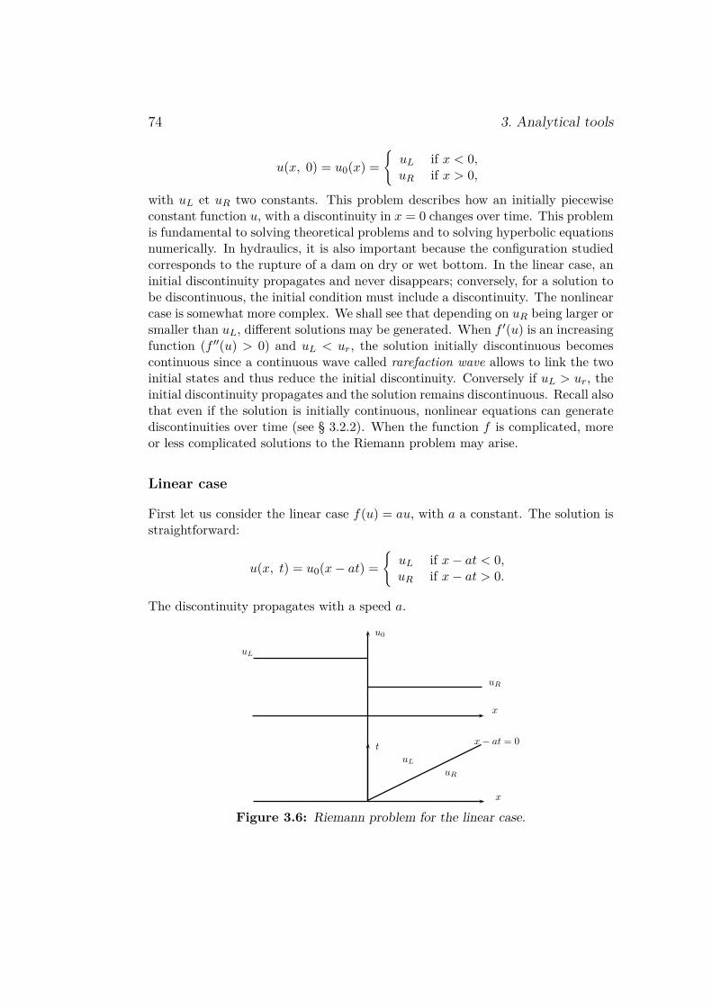
74 3. Analytical tools
u(x, 0) = u0(x) =uL if x < 0,uR if x > 0,
with uL et uR two constants. This problem describes how an initially piecewiseconstant function u, with a discontinuity in x = 0 changes over time. This problemis fundamental to solving theoretical problems and to solving hyperbolic equationsnumerically. In hydraulics, it is also important because the configuration studiedcorresponds to the rupture of a dam on dry or wet bottom. In the linear case, aninitial discontinuity propagates and never disappears; conversely, for a solution tobe discontinuous, the initial condition must include a discontinuity. The nonlinearcase is somewhat more complex. We shall see that depending on uR being larger orsmaller than uL, different solutions may be generated. When f ′(u) is an increasingfunction (f ′′(u) > 0) and uL < ur, the solution initially discontinuous becomescontinuous since a continuous wave called rarefaction wave allows to link the twoinitial states and thus reduce the initial discontinuity. Conversely if uL > ur, theinitial discontinuity propagates and the solution remains discontinuous. Recall alsothat even if the solution is initially continuous, nonlinear equations can generatediscontinuities over time (see § 3.2.2). When the function f is complicated, moreor less complicated solutions to the Riemann problem may arise.
Linear case
First let us consider the linear case f(u) = au, with a a constant. The solution isstraightforward:
u(x, t) = u0(x− at) =uL if x− at < 0,uR if x− at > 0.
The discontinuity propagates with a speed a.
x
x
t
u0
uL
uR
uL
uR
x − at = 0
Figure 3.6: Riemann problem for the linear case.

3.2 First-order hyperbolic differential equations 75
Nonlinear case
Convex flux (f ′′ > 0) In the general case (where f ′′ = 0), the Riemannproblem is an initial-value problem of the following form:
∂tu+ ∂x[f(u)] = 0,
u(x, 0) = u0(x) =uL if x < 0,uR if x > 0.
with uL and uR two constants. Assume that f ′′ > 0 (the case of a non-convex flowwill not be treated here). We will show that there are two possible solutions:
• a solution called rarefaction wave (or simple wave), which is continuous;
• a discontinuous solution which represents the spread of the initial disconti-nuity (shock).
Physically, only one of these solutions is possible and the choice will be dictatedby a condition (called entropy) depending on the respective value of uL and uR.Essentially, the idea is that shocks cause energy dissipation and cannot createenergy!
Rarefaction wave. Note first that this equation is invariant under thetransformation x → λx and t → λt. A general solution can be sought in the formU(ξ) with ξ = x/t. Substituting this general form into the partial differentialequation, we obtain an ordinary differential equation of the form:(
f ′(U(ξ)) − ξ)U ′ = 0.
There are two types of solution to this equation:
• rarefaction wave: (f ′(U(ξ)) − ξ) = 0. If f ′′ > 0, then f ′(uR) > f ′(uL) ;equation f ′(U) = ξ admits a single solution when f ′(uR) > ξ > f ′(uL). Inthis case, uL is connected to uR through a rarefaction wave: ξ = f ′(U(ξ)).Inverting f ′, we find out the desired solution
u(x, t) = f ′(−1)(ξ) ;
• constant state : U ′(ξ) = 0. This is the trivial solution u(x, t) = cte. Thissolution does not satisfy the initial problem.
The solution reads
u(x, t) =
uL if x
t≤ f ′(uL),
f ′(−1)(ξ) si f ′(uL) ≤ x
t≤ f ′(uR)
uR if xt
≥ f ′(uR).

76 3. Analytical tools
Shock wave. We have previously seen that weak solutions (discontinues) tothe hyperbolic differential equation (3.25) may exist. Assuming a discontinuityalong a line x = s(t) = st, we get: Jf(u)K = sJuK. The solution is then:
u(x, t) =uL if x < st,uR if x > st.
Then there is formation of a shock wave velocity s given by:
s = f(uL) − f(uR)uL − uR
.
Selection of the physical solution. Two cases may arise (remember thatf ′′ > 0). We call λ(u) = f ′(u) the characteristic velocity (see section below), whichis the slope of the characteristic curve (straight line) of the problem.
• 1st case: uR > uL. Since f ′′ > 0, then λ(uR) > λ(uL). At initial timet = 0, the two characteristic lines form a fan. Equation ξ = f ′(U(ξ)) admitsa solution over the interval λ(uR) > ξ > λ(uL). See Fig. 3.7;
• 2nd case: uR < uL. Characteristic lines intersect as of t = 0. The shockpropagates at rate λ(uR) < s < λ(uL). This last condition is called Laxcondition; it allows to determining whether the shock velocity is physicallyadmissible.
x
x
t
u0
uL
uR
uL
uR
x − mt = 0
x=
λ(u
L)t
x = λ(uR)t
Figure 3.7: Riemann problem for uR > uL.
Non-convex flux For some applications, the flux is not convex. An exampleis given by the equation of Buckley-Leverett, reflecting changes in water concen-tration ϕ in a pressure-driven flow of oil in a porous medium:
ϕt + f(ϕ)x = 0,

3.2 First-order hyperbolic differential equations 77
with f(ϕ) = ϕ2(ϕ2 + a(1 − ϕ)2)−1 and a a parameter (0 < a < 1). This fonctionhas an inflexion point. Contrary to the convex case, for which the solution involvesshock and rarefaction waves, the solution is here made up of compose de chocs etcompound wave) resulting from the superimposition of one shock wave and onerarefaction wave (LeVeque, 2002, see pp. 350–356).

78 3. Analytical tools
Exercises
Exercice 3.1 We would like to solve the following equation over [0, 1]:`ϵy′′ + y′ + y = 0,
with initial conditions y(0) = 1 and y(1) = 1. Show that there is no regularexpansion to this equation. Can you find the reason why the regular perturbationtechniques does not work here?
Exercice 3.2 (Homework)`The Boussinesq equation is used to calculate the level of an aquifer in the
ground; for example, as shown in Figure 3.8, a water flow in a channel, wherethe water height varies with time causes groundwater flow. For one-dimensionalproblem, the Boussinesq equation reads
θ∂h
∂t= Ks
∂
∂x
(h∂h
∂x
),
with θ soil porosity, Ks hydraulic conductivity, h water level. The boundaryconditions are
h(0, t) = h0(t),lim
x→∞h(x, t) = 0.
The initial condition is h(x, 0) = 0 for x ≥ 0. Reply to the following questions:
• put the Boussinesq equation in a dimensionless form;
• search how to write the similarity solutions when H0(t) = Atn (i.e., showthat solutions can be sought in the form h = tαH(ξ) with ξ = xt−β);
• show that the initial differential problem can be transformed into an ordinarydifferential problem in H;
• we consider the case where the level in the channel is constant H0 = A(n = 0). Show that the governing differential equation in H can be reducedto a quasi-linear equation of first order by making of the following changeof variable z = H/ξ2 and p = H ′/ξ;
• write this equation in the form dp/dz = f(p, z) with f a function to bedetermined;

3.2 First-order hyperbolic differential equations 79
h(x, t)h0
x
Figure 3.8: groundwater propagation.
• show that there is front propagation, c’est-à-dire a point xf where h(xf ) = 0and h = 0 beyond this point.
Exercice 3.3 Solve the initial value problem: `ux + ut = 0,
for x ∈ R and with u(x, 0) = cosx.
Exercice 3.4 Solve analytically, then approximately to order ϵ the following aequation
dy(x)dx
+ ϵy(x) = 1,
with boundary conditions y(0) = 1 and where ϵ = 0.01 is a small parameter.
Answer. The analytical solution is
y(x) = e−xϵ (ϵ+ exϵ − 1)ϵ
.
We use the following expansion y = y0 + ϵy1 + . . .. To order ϵ0, we have to solvey′
0 = 1 with y0(0) = 1, that is, y(x) = x + 1. To order ϵ1, we have to solvey′
1 + y0 = 0 with y1(0) = 0, that is, y1(x) = −x− 12x
2.As shown on Fig. 3.9, the deviation between the theoretical and approximate
solutions is low, even at order ϵ0. ⊓⊔
Exercice 3.5 Solve Huppert’s equation, which describes fluid motion over an ainclined plane in the low Reynolds-number limit:
∂h
∂t+ ρgh2 sin θ
µ
∂h
∂x= 0. (3.29)

80 3. Analytical tools
0 1 2 3 4 5
x
1
2
3
4
5
6
y(x
)
Figure 3.9: comparison between the theoretical solution (solid line) and approx-imate solution (to order ϵ0) y = x+ 1 (dashed line) over 0 ≤ x ≤ 5.
Note that this equation is obtained from the Navier-Stokes equations assumingthat the inertial terms are negligible and using the approximation of long wave(Huppert, 1982). The boundary conditions are given in Figure 3.10: it is therelease of a finite volume of fluid.
x
x
h0
x = `
Figure 3.10: initial flow configuration.
Answer. This is a nonlinear convection equation of the form: ∂th+ c(h)∂xh =0 with c(h) = ρgh2 sin θ/µ or equivalently ∂th + ∂xf(h) = 0 with f(h) =ρgh3 sin θ/(3µ).
This initial boundary-value problem can be solved straightforwardly. It isindeed a double Riemann problem, a first Riemann problem at x = 0 and anotherone x = ℓ. We must therefore seek weak solutions (shock) and rarefaction wavesthat are associated with this equation. For weak solutions with a discontinuity inx = s(t), there is a relation that gives h on both sides of x = s
sJhK = Jf(h)K (3.30)

3.2 First-order hyperbolic differential equations 81
as a function of s, the shock speed. Rarefaction waves are similarity solutions ofthe form H(ξ) with ξ = x/t. Here, substituting h(x, t) with H(ξ) into (3.29), weobtain
H′(−ξ + c(H)) = 0,which implies that we have either H′ = 0, or
H =√
µ
ρg sin θξ. (3.31)
h0
t
x
onde
dedé
tent
e
choc
bb
AO
Figure 3.11: characteristic curves.
When put in a characteristic form, (3.29) becomesdhdt
= 0 le long de dxdt
= c(h). (3.32)
It follows that initially the characteristics are straight lines, whose slope is givenby c(h0), as shown in Fig. 3.11.
At short times, there is
• a shock on the right. According to (3.28), we have
s0JhK = Jf(h)K,s0(0 − h0) = f(0) − f(h0),
s0 = f(h0)h0
= ρgh20 sin θ3µ
whose characteristic curve emanating from point A has the following equa-tion
x = ℓ+ s0t = ℓ+ 13ρgh2
0 sin θµ
t.

82 3. Analytical tools
• a rarefaction wave on the left. Point O is the apex of a fan made up ofstraight characteristic lines:
x = mt,
with m a real parameter varying from 0 to m0 = ρgh20 sin θ/µ.
h0
t
x
bb
AO
b
B
x=
s0t
x=
m0t
Figure 3.12: crossing of two characteristics.
The two characteristic lines x = m0t and x = ℓ+ s0t cross at point B and timetB
tB = ℓ
m0 − s0= 3
2µℓ
ρgh20 sin θ
.
The abscissa of B isxB = m0tB = 3
2ℓ.
The short-time solution is then (0 ≤ t ≤ tB)
h(x, t) =√
µ
ρg sin θx
tfor 0 ≤ x ≤ m0t, (3.33)
h(x, t) = h0 for m0t ≤ x ≤ ℓ+ s0t (3.34)h(x, t) = 0 for x > s(t) = ℓ+ s0t or x < 0. (3.35)
Note that the volume is well conserved over time.For t > tB, the flow depth on the right of x = s(t) is still 0, but leftwards, it
diminishes. According to (3.29), this flow depth is
hs =√
µ
ρg sin θs
t

3.2 First-order hyperbolic differential equations 83
which leads to the following shock speed
sJhK = Jf(h)K,s(0 − hs) = f(0) − f(hs),
s = f(hs)hs
= ρgh2s sin θ3µ
= 13s
t.
Integrating this equation, we find that the characteristic curve associated with theshock is
s(t) = xB
(t
tB
)1/3= 3
2
(23ρgh2
0ℓ2 sin θµ
t
)1/3
= At1/3,
with A =(
94
ρgh20ℓ2 sin θ
µ
)1/3. The long-time solution is then (t > tB)
h(x, t) =√
µ
ρg sin θx
tfor 0 ≤ x ≤ At1/3, (3.36)
h(x, t) = 0 pour x > s(t) = At1/3 for x < 0. (3.37)
Exercice 3.6 The Emden-Fowler equation arises in the context of equilibrium- `mass distribution of a cloud of gas with adiabatic exponent
y + 2xy + yn = 0,
with n = 5 (corresponding to an adiabatic exponent 6/5).
• Seek similarity variables (hint: show that the equation is invariant understretching group).
• Plot the phase portrait after a change of variable (with the similarity vari-able).
• Try to find an analytical solution.


4Propriétés des fluides
4.1 Diffusion
4.1.1 Équations de diffusion
Une propriété assez générale aux fluides est la diffusion liée à l’agitation moléculaireet/ou au mouvement fluide. Si l’on place dans de l’eau un volume fini d’une solutiond’une espèce diffusante (c’est-à-dire qu’elle ne va pas sédimenter tout de suite)comme par exemple de l’encre ou du sucre fin, on va observer une redistribution etun transport progressif de cette espèce dans tout le volume. Il en est de même sil’on chauffe localement un fluide, la chaleur va se propager progressivement danstout le volume. Dans les deux cas de figure, on parle de diffusion.
Un cas typique de diffusion est rencontré lorsqu’il y a un gradient de concen-tration. Par exemple, soit n(x, t) le nombre de particules en x, à l’instant t le longd’un barreau de section S. Expérimentalement, on observe que le flux de partic-ules à travers ce barreau peut être défini à l’aide d’une relation dite (première) loide Fick1
J = δn
Sδt= −Ddn
dx,
avec D le coefficient de diffusion moléculaire (supposé constant), S la surface dubarreau, δn la différence entre le nombre de particules entrant en x et sortant enx + ∆x (voir figure 4.1) pendant δt. Cette loi empirique est l’équivalent de la loid’Ohm pour une résistance : I = U/R ; le coefficient de diffusion correspond àla conductivité (1/R), δn à la différence de potentiel U , et I et J sont deux «courants ».
1Adolf Eugen Fick (1829–1901) était un médecin allemand spécialisé en physiologie. Ilproposa la loi qui porte aujourd’hui son nom et qui fut établie à partir d’expériences dediffusion d’un gaz à travers une membrane. Il est à l’origine des lentilles de contact et despremières mesures du débit cardiaque.
85

86 4. Propriétés des fluides
x x + dx
n(x) n(x + dx) = n + δn
S
J
Figure 4.1: bilan de matière dans un barreau.
Si on fait un bilan dans le barreau considéré comme un milieu unidimensionnelet qu’on applique le principe « variation de n au cours du temps = ce qui entre– moins de ce qui sort », on aboutit à une équation de diffusion pour n(x, t), quiest en tout point semblable à l’équation de la chaleur
∂n
∂t= D
∂2n
∂x2 . (4.1)
L’exemple typique de solution est celle obtenue en considérant qu’à l’instant t = 0,on lâche une quantité N de particules, qui seraient concentrées initialement dansune bande infiniment fine autour de x = 0. Les particules vont ensuite se propagerdans les deux directions. Comme on peut le montrer (voir annexe 2), la solutionmathématique à l’équation de diffusion est une gaussienne
n(x, t) = N
2√πDt
e− x24Dt .
Comme le montre la figure 4.2, l’effet de la diffusion moléculaire est d’adoucirle profil de concentration en n : au cours du temps, le profil est de plus en plusplat.
Comme pour la loi de Fourier vue (voir annexe 2), on peut généraliser cette loiscalaire pour obtenir une loi tensorielle (en dimension 3) en interprétant la dérivéecomme un gradient :
J = −D∇n,où J est appelé aussi le vecteur « densité de courant » et cette équation est appeléeseconde loi de Fick. On peut obtenir une équation linéaire tridimensionnelle dediffusion
∂n
∂t= −D∇ · J.
Aussi bien pour les cas scalaire que tridimensionnel, on considère que la diffusiona lieu dans un fluide au repos. Si le fluide est en mouvement, il faut tenir comptede l’advection de matière ; mathématiquement, on remplace la dérivée locale parrapport au temps par une dérivée totale
dndt
= ∂n
∂t+ u · ∇n = D∇ · J = Dn,
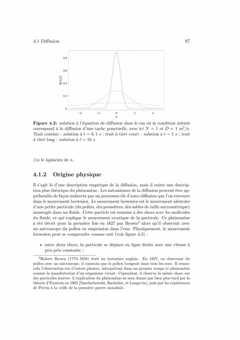
4.1 Diffusion 87
-4 -2 0 2 4
x
0
0.2
0.4
0.6
0.8n(
x,t)
Figure 4.2: solution à l’équation de diffusion dans le cas où la condition initialecorrespond à la diffusion d’une tache ponctuelle, avec ici N = 1 et D = 1 m2/s.Trait continu : solution à t = 0, 1 s ; trait à tiret court : solution à t = 1 s ; traità tiret long : solution à t = 10 s.
n le laplacien de n.
4.1.2 Origine physique
Il s’agit là d’une description empirique de la diffusion, mais il existe une descrip-tion plus théorique du phénomène. Les mécanismes de la diffusion peuvent être ap-préhendés de façon indirecte par un processus dit d’auto-diffusion que l’on retrouvedans le mouvement brownien. Le mouvement brownien est le mouvement aléatoired’une petite particule (du pollen, des poussières, des sables de taille micrométrique)immergée dans un fluide. Cette particle est soumise à des chocs avec les moléculesdu fluide, ce qui explique le mouvement erratique de la particule. Ce phénomènea été décrit pour la première fois en 1827 par Brown2 alors qu’il observait avecun microscope du pollen en suspension dans l’eau. Physiquement, le mouvementbrownien peut se comprendre comme suit (voir figure 4.3) :
• entre deux chocs, la particule se déplace en ligne droite avec une vitesse àpeu près constante ;
2Robert Brown (1773–1858) était un botaniste anglais. En 1827, en observant dupollen avec un microscope, il constata que le pollen bougeait dans tous les sens. Il renou-vela l’observation sur d’autres plantes, interprétant dans un premier temps ce phénomènecomme la manifestation d’un organisme vivant. Cependant, il observa la même chose surdes particules inertes. L’explication du phénomène ne sera donné que bien plus tard par lathéorie d’Einstein en 1905 (Smoluchowski, Bachelier, et Langevin), puis par les expériencesde Perrin à la veille de la première guerre mondiale.

88 4. Propriétés des fluides
• la particule est accélérée instantanément lorsqu’elle est percutée par unemolécule ou bien rencontre une paroi. Sa trajectoire marque alors un change-ment net de direction.
O
M1
M2M3
Mn
Mn+1
(a) (b)Figure 4.3: idéalisation du mouvement brownien. (a) vue générale ; (b) agran-dissement.
Puisque la particule supposée au repos réalise des déplacements aléatoires augré des collisions, il n’y a pas de raison pour qu’il y ait un sens de déplacementfavorisé, donc en valeur moyenne, le déplacement r(t) est nul, ce que l’on note par
⟨r(t)⟩ = 0
où les crochets ⟨·⟩ renvoient à une moyenne (dans le temps). En revanche, lemoment du second ordre3 ou la variance du déplacement n’est pas nul. Ce moments’écrit ⟨r2(t)⟩ et peut s’interpréter comme la moyenne du carré du déplacement.On va montrer assez simplement que ce moment du second ordre s’écrit4
⟨r2(t)⟩ = nℓ2,
avec n le nombre de chocs subit par la particule. On suppose ici qu’en moyenne,tous les bouts de trajectoires sont de même longueur ℓ. Il s’ensuit aussi que si tcdésigne le temps moyen entre deux collisions, on a n = t/tc (on a aussi tc = ℓ/w,
3Si f désigne une densité de probabilité d’une variable X, alors la moyenne de X est∫xf(x)dx et est appelé moment du premier ordre ; le moment d’ordre n est simplement∫xnf(x)dx.
4Il suffit pour cela d’écrire qu’à l’instant t, r(t) = OMn =∑n
i=0 Mi−1Mn, puis decalculer la moyenne de ⟨r2(t)⟩ en faisant la décomposition.

4.1 Diffusion 89
avec w la vitesse de la particule entre chaque collision), d’où
⟨r2(t)⟩ = nℓ2 = ℓ2
tct.
Si on définit le coefficient de diffusion comme étant D = ℓ2/tc = wℓ, on trouve que⟨r2(t)⟩ = Dt. La particule « diffuse » donc en
√t autour de sa position initiale
r = 0.Notons que le raisonnement réalisé en dimension 2 peut être mené dans le cas
d’une propagation aléatoire dans une seule direction de l’espace, ce qui va perme-ttre d’apporter un éclairage différent au problème de la figure 4.1, où l’on étudiaitun transport de particules dans un barreau. Considérons une particule parmi les nparticules présentes dans le barreau et supposons qu’elle soit en mouvement aléa-toire. La probabilité qu’elle aille dans une direction équivaut à celle qu’elle ailledans la direction opposée ; la probabilité qu’elle change de direction à l’instant test indépendante de tout ce qui a pu se passer jusqu’à l’instant t. La direction estdonc aléatoire et peut prendre deux valeurs équiprobables ϵ = ±1 ; le temps t estcontinu ; la vitesse de la particule est supposée constante et égale à w. On écritdonc tout cela sous forme mathématique
P (x− δx, t+ δt|x, t) = 12,
P (x+ δx, t+ δt|x, t) = 12,
avec δx et δt de petits intervalles d’espace et temps, qui sont fixes. Ce que l’onpeut traduire : la probabilité que la particule soit à l’instant t+δt en x−δx sachantqu’elle était en x à l’instant t vaut 1/2. En se servant des lois de composition desprobabilités5
P (x, t+ δt) = P (x, t+ δt|x− δx, t)P (x− δx, t) + P (x, t+ δt|x+ δx, t)P (x+ δx, t)
= 12P (x− δx, t) + 1
2P (x+ δx, t).
En faisant un développement limité au second ordre6 en x, on trouve que P vérifiel’équation
P (x, t+ δt) − P (x, t) = 12δx2∂
2P
∂x2 ,
puis un développement au premier ordre en δt amène finalement à
∂P
∂t= δx2
2δt∂2P
∂x2 .
5Rappelons que P (x, y) = P (x|y)P (y) par définition de la probabilité conditionnelle.6Rappel f(x+ δx) = f(x) + δxf ′(x) + δx2f ′′(x)/2 + · · · .
90 4. Propriétés des fluides
On note que c’est la même équation que celle de la chaleur ou celle de la diffusion(4.1) sous réserve que δx2/δt soit constant. On pose donc δx =
√2Dδt. On aboutit
donc à l’équation suivante pour la probabilité P (x, t)
∂P
∂t= D
∂2P
∂x2 ,
qui est une forme particulière de l’équation de Fokker-Planck. Une solution decette équation est la loi de Gauss. Puisqu’en moyenne le déplacement moyen estnul (aucune direction favorisée), on déduit que
P (x, t) = 1√4πDt
e− x24Dt .
On note dans ce cas particulier la correspondante des équations et des solutionspour n(x, t) et P (x, t).
Un point important également à noter dans notre explication du mouvementbrownien est qu’encore une fois, c’est l’agitation thermique des atomes qui expliquele comportement observé à l’échelle macroscopique. L’agitation est donc respon-sable à la fois d’une force continue (force de viscosité) et d’une force erratique(collisions donnant naissance au mouvement brownien). C’est cette analyse qui apermis à Einstein7 de calculer le coefficient de diffusion d’une particule sphériquede rayon a dans un fluide newtonien de viscosité µ
D = kT
6πµa,
qui montre que le coefficient de diffusion est un rapport entre l’énergie cinétiquefluctuante kT et la force de frottement visqueuse 6πµa.
Dans les expériences de Brown, on a précisé que le mouvement brownien af-fecte des particules de petite taille, typiquement de taille micrométrique pour uneparticule dans de l’eau. On peut caractériser plus finement l’échelle de taille etles caractéristiques du fluide pour lesquelles le mouvement brownien est impor-tant. Cela peut se faire par exemple en considérant la (seconde) loi de Fick pourcalculer la diffusion de particules dans un fluide en mouvement avec une vitessecaractéristique u∗
∂n
∂t︸︷︷︸variation locale
+ u · ∇n︸ ︷︷ ︸convection
= Dn︸ ︷︷ ︸diffusion
.
7Albert Einstein (1879-1955) a été le physicien le plus célèbre du xxe siècle siècle,principalement pour ses travaux sur la relativité, qui remettait en cause notre conceptiondu monde. Einstein a également eu des contributions importantes en physique des flu-ides en expliquant le mouvement brownien et en calculant la viscosité équivalente d’unesuspension diluée de particules dans un fluide newtonien.

4.1 Diffusion 91
Si l’on compare dans cette équation différentielle, la part jouée par la convectionet celle jouée par la diffusion, on peut former un rapport sans dimension appelénombre de Péclet8
Pe = convectiondiffusion
∼ u∗n/ℓ∗Dn/ℓ2∗
∼ u∗ℓ∗D
,
où ℓ∗ est une échelle caractéristique du système étudié (taille de la particule ou libreparcours moyen). Lorsque Pe ≫ 1, la convection l’emporte sur la diffusion. Lesparticules sont donc transportées (advectées) par le fluide. Dans le cas contraire,lorsque Pe ≪ 1, la diffusion l’emporte sur la convection.
8Jean Claude Eugène Péclet (1793–1857) était un physicien français, essentiellementtourné vers l’enseignement. Il est à l’origine de l’École Centrale des Arts et Manufactures.

92 4. Propriétés des fluides

APhase portrait
A.1 IntroductionA number of nonlinear equations of first order as well as second-order autonomousequations can be cast in the following form:
dydx
= f(x, y)g(x, y)
, (A.1)
with f and g two functions that may vanish. The points that are both zeros off and g are called singular points 1 since the differential term dy/dx is a prioriindeterminate at these points. The behavior of the integral curves depends stronglyon the structure of curves f(x, y) = 0 and g(x, y) = 0 around these criticalpoints, c’est-à-dire the multiplicity of critical curves generated by the equationsf(x, y) = 0 and g(x, y) = 0 and by the sign of f/g in the different areas delineatedby these critical curves.
The simplest case is encountered when, near the singularity, it is possible tolinearize Equation (A.1). We can then write: f(x, y) = ax + by + o(x, y) etg(x, y) = cx+ dy+ o(x, y). Let us assume that ad− bc = 0 and these coefficientsare not all zero. There are two critical curves in the vicinity of the singularity:
• y = −ax/b where the curves admit a horizontal tangent;
• y = −cx/d where the curves admit a vertical tangent.
Introducing dummy variable t, we can transform (A.1) into the matrix form:
ddt
u = M · u, with M =[c da b
]. (A.2)
1They are also called critical points or equilibrium points.
93

94 A. Phase portrait
We seek a solution in the form v = v0 exp(λt), with v0 the initial-condition vector(at t = 0). We deduce that λ must be an eigenvalue of the matrix M and v0 anassociate eigenvector; λ is solution to the second order equation λ2 − 2hλ+ k = 0,with 2h = b+ c and k = det M = −ad+ bc, that is:
λ = h±√h2 − k.
The principal directions principales are: b − c ∓√
(b− c)2 + 4ad. Depending onthe value taken by λ, different behaviors arise:
• when ∆ = h2 − k > 0 and k > 0, the two eigenvalues are real and of thesame sign. Assume that h > 0, then the two eigenvalues are positive, whichmeans that either both solutions to (A.2) tend to 0 as t → −∞ (resp. whenh < 0, the solutions tend to 0 as t → +∞). Hence, if every initial conditionlies on one of the principal axes, each solution tends to the origin point, thesolution is a part of a straight line with slope equal to one of the principaldirections. What happens if the initial condition does not lie on one of theprincipal directions? Let us assume that an integral curve tends towards theorigin point. The limit of dy/dx at 0 in the equation (A.1) is not defined.Applying Rule’s Hospital (see below), the slope of the solution at point Omust satisfy:
m = a+ bm
c+ dm,
i.e., m = b − c ±√
(b− c)2 + 4ad and m coincide with one of the maindirections. Given the sign of dy/dx around the origin point, only one ofthese solutions is possible: the curves reach the origin point, following anasymptotic curve of equation y = mx. This singularity is called a node.Figure A.1 shows an example.
• if ∆ > 0 and k > 0, the two eigenvalues are real and of opposite sign.The two solutions of system (A.2) behave differently when t → ∞: onetends towards the singular point while the other tends to infinity. There arealways two curves that pass through the singular point and that coincidewith the principal directions. If now the initial point (initial condition ofthe differential equation) does not lie on one of the principal directions,then it is not possible to find an integral curve emanating from that pointto the singular point because of the sign of dy/dx in the close vicinity of thesingular point. The paths diverge when approaching the singular point. Werefer to this point as a saddle. Figure A.2 shows an example.
• if ∆ = 0, the singular point is a node.
• if ∆ < 0, both eigenvalues are imaginary. The curves coiled like a spiralaround the singular point. This point is called focal point. Figure A.3 showsan example.

A.1 Introduction 95
♣ Example. – When solving the equation:
dydx
= x+ 2y2x+ y
, (A.3)
we find out that there are two eigenvalues 3 and 1 associated with principal direc-tions 1 and et −1 respectively. It is a node.
♣ Example. – When solving the equation:
dydx
= 2x+ y
x+ 2y, (A.4)
we find out that there are two eigenvalues 3 and −1 associated with principaldirections 1 and et −1 respectively. It is a saddle.
♣ Example. – When solving the equation:
dydx
= 2x+ y
x− y, (A.5)
we find out that there are two complex eigenvalues (3± ı√
3)/2. It is a focal point.
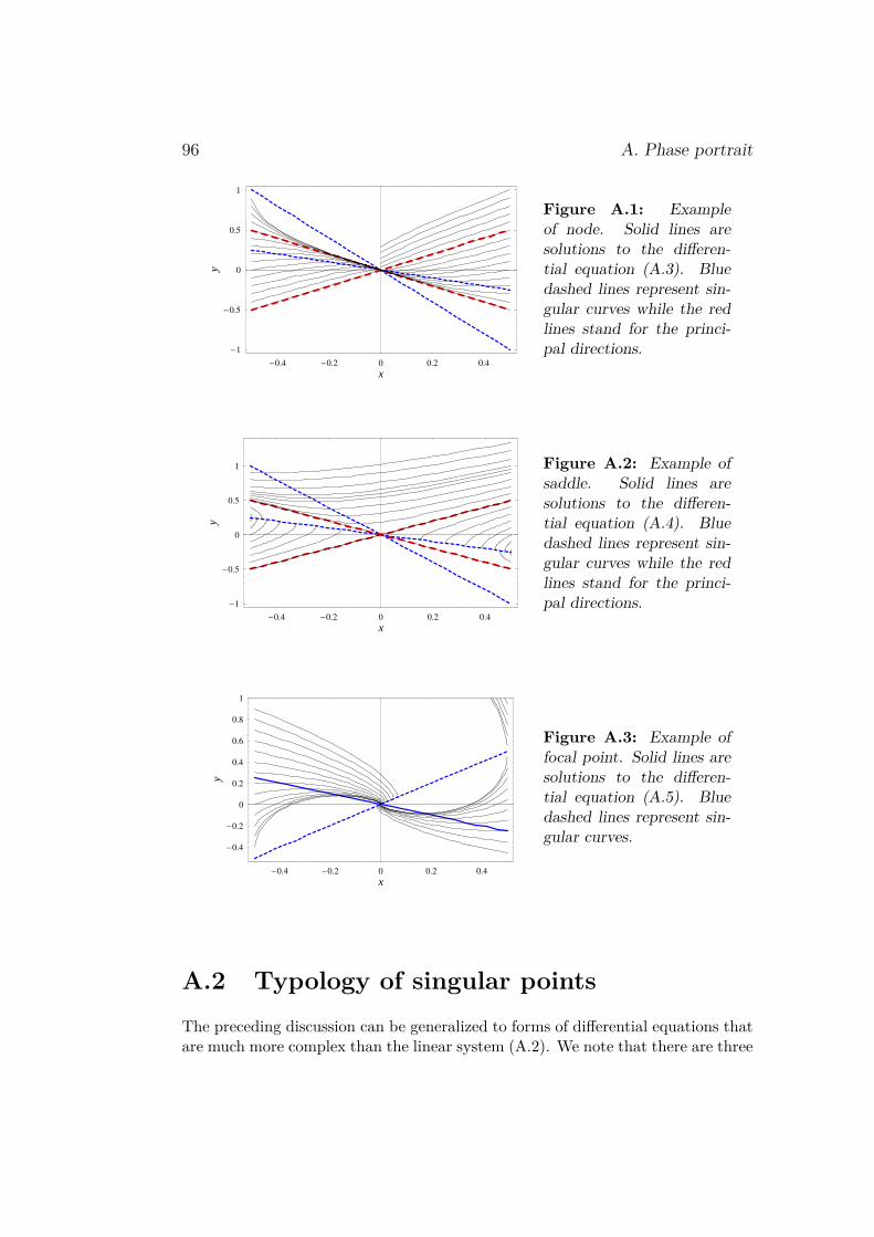
96 A. Phase portrait
-0.4 -0.2 0 0.2 0.4
x
-1
-0.5
0
0.5
1
yFigure A.1: Exampleof node. Solid lines aresolutions to the differen-tial equation (A.3). Bluedashed lines represent sin-gular curves while the redlines stand for the princi-pal directions.
-0.4 -0.2 0 0.2 0.4
x
-1
-0.5
0
0.5
1
y
Figure A.2: Example ofsaddle. Solid lines aresolutions to the differen-tial equation (A.4). Bluedashed lines represent sin-gular curves while the redlines stand for the princi-pal directions.
-0.4 -0.2 0 0.2 0.4
x
-0.4
-0.2
0
0.2
0.4
0.6
0.8
1
y
Figure A.3: Example offocal point. Solid lines aresolutions to the differen-tial equation (A.5). Bluedashed lines represent sin-gular curves.
A.2 Typology of singular pointsThe preceding discussion can be generalized to forms of differential equations thatare much more complex than the linear system (A.2). We note that there are three

A.3 Computation of the asymptotic curve 97
possible types of behavior:
• node where the integral curves (there exists an infinity of such curves) aredirected towards the singular point, usually following an asymptotic curvethat can be deduced from the differential equation;
• saddle where the integral curves diverge as they approach the singular point,except one who is able to cross it;
• focal point where the curves wrap up like spirals or make loop around thesingular point.
Figure A.4: Typology of singular points where there are two critical curves.After (Jones, 1953).
In the general case, the behavior of functions is a combination of these threebasic forms, which is more or less complex depending on the number of criticalcurves f = 0 and g = 0. Figure A.4 recalls the possible behaviors when thereare two critical curves. Figure A.5 shows the possible combinations when thereare three critical curves (two corresponding to f = 0 et a single one to g = 0).Figure A.6 shows the possible combinations when four critical curves, two of whichcoincide with the coordinate axes.
A.3 Computation of the asymptotic curveWhen the singularity is a node, there is an asymptotic curve to which any curvepassing through the singularity tends. Similarly, when the singular point is a

98 A. Phase portrait
Figure A.5: Typology of singular points where there are three critical curves.After (Jones, 1953).
Figure A.6: Typology of singular points where there are four critical curves.After (Jones, 1953).
saddle, there is a (single) curve solution that arrives at the singular point. Theexceptional curve is called separatrix. because it also separates two regions ofspace, each characterized by a specific behavior near the singular point. We canuse several methods to work out the equation of this curve.
A.3.1 Numerical computation
Using l’Hôpital’s rule, we can obtain the asymptotic curve toward which the inte-gral curves moving towards a node converge or the single curve passing through a

A.3 Computation of the asymptotic curve 99
saddle. Indeed we can write:
F (x) = f(x, y(x)) and G(x) = g(x, y(x)).
By making a first-order expansion around a singular point xs, we have:
ys + xys + · · · =xFs + x2
2 Fs + · · ·xGs + x2
2 Gs + · · ·=
Fs + x2 Fs + · · ·
Gs + x2 Gs + · · ·
,
with ys = y(xs) et ys = y(xs). Computing Fs requires the computation of com-pound derivatives:
F = ∂f
∂x+ y
∂f
∂y,
F = ∂F
∂x+ y
∂F
∂y+ y
∂F
∂y.
We do the same withG. We wish to compute the series expansion of the asymptoticcurve at the singular point, that is, an equation of the form y = ys +m(x− xs) +p(x− xs)2/2, with m = ys = y(xs) and p = ys = y(xs). To order 0, we must solvethe second-order equation:
m = fx +m fy
gx +m gy, (A.6)
to find m. Once m is known, we can infer p, which is solution to the followingequation:
Fs = mGs + 2pGs. (A.7)
♣ Example. – Let us consider the differential equation
dydx
= x+ 3xy + 3(1 − y)y3x(2x+ 3y)
.
We would like to determine how the integral curves behave close the origin point(which is singular). We find:
F (0) = 1 + 3m et G(0) = 0,
and the solution to (A.6) is m = −1/3. To order 1, we get
F (0) = −83p et G(0) = 6,
and the solution to ( (A.7) is p = 2/9. The equation of the asymptotic curve isthen:
y = −13x
(1 − 2
3x+ · · ·
).

100 A. Phase portrait
0 0.2 0.4 0.6 0.8 1x
-0.3
-0.2
-0.1
0
0.1
0.2
y
Figure A.7: Convergence of integral curves towards the asymptotic curve.
A.3.2 Analytical calculation
The separatrix is a curve, which is solution to the differential equation (A.1) for allLie groups admitted by the same equation. An implicit curve equation ϕ(x, y) = 0is invariant under a Lie group X = ξ∂x + η∂y if Xϕ = 0. Using the condition
Xϕ = ξ∂xϕ+ η∂yϕ = 0,
we deduce that ϕ is also solution to the following first-order differential equation
y′ = η(x, y)ξ(x, y)
.
The equation of the separatrix is then obtained by substituting y′ by η/ξ into(A.1) (Dressler, 1983; Bluman, 1990) :
η(x, y)ξ(x, y)
= f(x, y)g(x, y)
.
To find the equation of the separatrix, we must then find all groups that leaveEquation (A.1) invariant. This is beyond the scope of the lecture notes and wemention this technique just for completeness.
♣ Example. – Let us consider the differential equation
y′ = y(x− y2)x2 ,
which is invariant under transformation x1 = λx and y1 =√λy, whose infinitesimal
generator is X = 2x∂x + y∂y. We then deduce ξ = 2x and η = y. The equation ofthe separatrix is
y
2x= y(x− y2)
x2 ,

A.4 Singular points located at infinity 101
or, equivalently,y2 = x
2.
⊓⊔
A.4 Singular points located at infinityIn many cases, we have f(x, y) → ∞ and g(x, y) → ∞ when x → ∞ and y → ∞,which implies that the behavior of dy/dx is indefinite there. One way to find theproper limit is to use the dominant-balance technique, i.e. y ≪ x, y ∼ x, or y ≫ x,then integrate the resulting differential equation to check whether the assumptionis consistent a posteriori or not. In some cases, singular points expelled to infinitymay actually represent a single point; a change of variable can usually show that(Lacey et al., 1982). For example, with the following variable change
x1 = x
x2 + y2 et y1 = − y
x2 + y2 ,
then by analyzing behavior at (0, 0) in the (x1, y1) plane, we can determine thebehavior of a singular at infinity (note that it is equivalent to making the changez1 = 1/z with z = x+ ıy).
♣ Example. – Let us consider the differential equationdydx
= 3y(x− 2y)(1 − 3x)y − x− x2 ,
for which we consider one of the following possibilities when x → ∞ and y → ∞:
• y ≪ x, then we find y ∝ 3y/x, i.e., y ∝ x3, which contrasts with the initialassumption;
• y ∼ x, then we set y ∝ mx, we deduce m = 4/3, which is consistent withour assumption;
• y ≫ x, then y/y ∝ 2y/x), i.e. y ∝ x2, which is consistent with our assump-tion.
For the first quadrant (x, y) > 0, x → ∞ and y → ∞, there are two singular pointsat infinity corresponding to two asymptotic curves y = 4x/3 and y = x2. For thesecond quadrant x → −∞ and y → ∞, there is one singular point correspondingto the curve y = x2, identical to the asymptotic curve we have found previously.It is in fact the same point and in practice, this means that one path may escapefrom the first quadrant along the curve y = x2 to return via the second quadrantand following the same curve. To show this, we can make the change of variable
u = 1x
and v = x2
y,
102 A. Phase portrait
such that both singular points of the first problem collapse onto a single pointA(0, 1). We then conclude:
dvdu
= v (2 − (5 + 2 u) v)3 + u (−1 + v) + u2 v
.
Point A is not a singular point of this equation; therefore, for A and for points inthe near vicinity of A, only one curve passes.
A.5 Singular points with horizontal/verticaltangent
We can find differential equations with singularities satisfying m = 0 or m = ±∞and in this case, the behavior is deduced by approximation and integration of thesolution (argument like the one used in the dominant balance technique).
♣ Example. – Let us consider the differential equation:
dydx
= 8 − 3xx(4 − x) − 2
y, (A.8)
for which we note that the denominator vanishes at A− (2−√
2, 0) and A+ (2+√
2,0), which are two singular points (nodes). The numerator vanishes at A0 (8/ 3,0), which corresponds to an extremum in the integral curve. The solution has thefollowing behavior:
A− A0 A+numerator + | + | − | −denominator − | + | + | −function − | + | − | +
The behavior around the nodes is then given by:
• for A−, we get:dydx
≈ ny
x− xA−,
with xA− = 2 −√
2 and n = (8 − 3xA−)/(xA+ − xA−) = 3/2 + 1/√
2 ≈2, 20 > 1. After integration, we find: y = c(x−xA−)n, with c an integrationconstante, thus at point A−, the curve admits a horizontal tangent.
• for A+, we have:dydx
≈ n′ y
x− xA+,

A.5 Singular points with horizontal/vertical tangent 103
avec n′ = (3xA+ − 8)/(xA+ − xA−) = −3/2 + 1/√
2 ≈ 0, 79 < 1. Afterintegration, we get: y = c|xA+ − x|n′ , thus at point A+, the curve admits avertical tangent.
Note that in this case, there is an analytic solution of the form:
y(x) = c|2 − ax+ x2|3/2 exp[−
√2 arctanhx− 2√
2
].
The result (numerical integration) is reported on the following figure. Note thatthe vertical tangent at point A+ is not very apparent because the interval overwhich the derivative is very large is narrow. ⊓⊔
0 0.5 1 1.5 2 2.5 3 3.5
x
-1
0
1
2
3
y
Figure A.8: Solution to equation (A.8).
♣ Example. – Let us consider the differential equation:
dydx
= 6y(2y − x)2q2 + 6yx+ x
.
It is singular at point O and A (0, − 1/2) At O, we find that m = 0. To work outthe asymptotic-curve equation, we try to approximate the solution. We assumex ≪ y when y → 0. This therefore gives
dydx
= 6y(2y − x)2q2 + 6yx+ x
≈ 12y2
x,
whose first integral is the family of curves
x = K exp(
− 112y
),
with K an integration constant.


BApproximation
B.1 DefinitionsWe are concerned with the scalar function (u, ϵ), which takes value x on an intervalD and depends on a parameter ϵ over an interval I: 0 < ϵ < ϵ1.
The notationu(x, ϵ) = O(v(x, ϵ)) sur I (B.1)
means that for all x over D, there exists a number k(x) such that
u(x, ϵ) ≤ k(x)|v(x, ϵ)|, pour tout ϵ ∈ I.
Similarly we haveu(x, ϵ) = O(v(x, ϵ)) quand ϵ → 0,
for any x of D, when there exists a positive real k(x) and a neighborhood N ofϵ = 0 such that u(x, ϵ) = k(x)|v(x, ϵ)| for any ϵ over I. The relation (B.1) is saidto be uniformly valid when k does not depend on x.
♣ Example. – The relation
1x+ ϵ
= O(1),
is correct because if we take k(x) = 1/x and since (x + ϵ)−1 < x−1, the relationu(x, ϵ) < k(x)×1 holds. However, this relation is not uniformly valide since thereis no constant k such that u(x, ϵ) < k × 1. ⊓⊔
The notation u = O(v) does not mean that u and v must have the same orderof magnitude. This notation implies tat u is bounded. If u and v have the sameorder of magnitude, then the limit u/v (when ϵ → 0) exists and is finite; we haveu = O(v) and v = O(u). We can make use of the following notation u = ord(v)(this notation is, however, not universally accepted).
105

106 B. Approximation
u(x, ϵ) = o(v(x, ϵ)) quand ϵ → 0 (B.2)means that for any x over D and for any constant k > 0, there is an interval Nϵ
(0 < ϵ < ϵ1(x, k)) such that
u(x, ϵ) ≤ k|v(x, ϵ)|, for any ϵ ∈ Nϵ.
u becomes arbitrarily small compared to |v|. We also note that u ≪ v. Therelation (B.2) is said to be uniformly valid if ϵ1 depends on k, but not on x.
A sequence of functions ϕn(ϵ) is called asymptotic series if
ϕn+1(ϵ) = o(ϕn(ϵ)) quand ϵ → 0.
♣ Example. – The sequence ϕn(ϵ) = ϵn−1 with n = 1, 2, . . . is an asymptoticseries. ⊓⊔
For a function (u, ϵ), its asymptotic expansion to order N means that whenϵ → 0, we are able to build a function
∑Nn=1 un(x)ϕn(ϵ) such that
u(x, ϵ) −N∑
n=1un(x)ϕn(ϵ) = o(ϕM ) quand ϵ → 0,
for M = 1, 2, . . . , N and where ϕn(ϵ) is a sequence of functions.When the function u is known and if the asymptotic series ϕn(ϵ) is specified,
we can easily construct the sequence of functions un(x)
u1(x) = limϵ→0
u(x, ϵ)ϕ1(ϵ)
,
u2(x) = limϵ→0
u(x, ϵ) − u1(x)ϕ1(ϵ)ϕ2(ϵ)
,
uk(x) = limϵ→0
u(x, ϵ) −∑k−1
n=1 un(x)ϕn(ϵ)ϕk(ϵ)
.
B.2 Regular perturbation techniquesLet us consider a projectile launched vertically from the Earth surface (sphere ofradius R). Its equation of motion is
d2z
dτ2 = − gR2
(z +R)2 , (B.3)
with g gravitational acceleration, τ > 0 the time, and with the initial conditionsz(0) = 0 and z(0) = v0. This problem is formally equivalent to
d2y
dt2= − 1
(ϵy + 1)2 , (B.4)

B.3 Non regular techniques 107
where ϵ = v20/Rg is a small parameter (ϵ ≪ 1), t = τ/T∗, z = y/L∗, T∗ = v0/g,
and L∗ = v20/g. We seek an asymptotic approximation to
y = y0 + ϵy1 + ϵ2y2 + . . .
Substituting this expression into (B.3), we have
1 +(y1
′′(t) − 2y0(t))ϵ+
(3y0(t)2 − 2y1(t) + y2
′′(t))ϵ2 + + . . . = −y0
′′(x).
To order ϵ0, we havey′′
0 + 1 = 0,
whose solution isy0 = t− 1
2t2.
To order ϵ, we gety′′
1 = 2y0 = 2t− t2,
whose solution isy1 = 1
12
(4t3 − t4
).
To order ϵ2, we get
y′′2 = 2y1 − 3y3
0 = 112t2(7t2 − 28t+ 36
),
whose solution isy2 = 1
360
(−7t6 + 42t5 − 90t4
).
The second-order approximation is then
y ∼ t− 12t2 + ϵ
12
(4t3 − t4
)+ ϵ2
360
(−7t6 + 42t5 − 90t4
).
B.3 Non regular techniquesLet us consider the following differential equation [0, 1]
(x+ ϵf)f ′ + f = 1,
with boundary condition f [1] = 2. Note that at x = −ϵf , the differential problembecomes singular. We use the following expansion
f = f0 + ϵf1 + ϵ2f2 + . . .
After substitution, we find that to order 0, we have
−1 + f0 + xf ′0 = 0,

108 B. Approximation
(a) 0.0 0.5 1.0 1.5 2.0 2.5
-0.4
-0.2
0.0
0.2
0.4
(b) 0.0 0.5 1.0 1.5 2.0 2.5
-0.4
-0.2
0.0
0.2
0.4
Figure B.1: Solution to Equation (B.4); dashed line: numerical solution, dashedline (a) solution to order ϵ0; dotted line (b) solution to order ϵ. Computation donefor ϵ = 0.1.
subject to the condition f0(1) = 2, which yields: f0(x) = (1 + x)/x. To order 1,we find
f1 + xf ′1 = 1 + x
x3 ,
subject to the condition f1(1) = 0, which gives: f1(x) = (3x2 − 2x− 1)/(2x3). Toorder 1, we get
9 + 4x
+ 2x4f2 + 2x5f ′2 = x(2 + 3x),
subject to the condition f2(1) = 0, which gives: f2(x) = (1 + 3x−x2 − 3x3)/(2x5).We finally obtain
f(x) = 1 + x
x+ ϵ
3x2 − 2x− 12x3 + ϵ2
1 + 3x− x2 − 3x3
2x5 + o(ϵ2). (B.5)
This approximation is asymptotic when x is fixed and ϵ → 0, but is no longerasymptotic when x = O(ϵ1/2). Indeed, the second term in the approximation,which should be O(ϵ) becomes O(1). To address this issue more carefully, we

B.3 Non regular techniques 109
can compare the approximate solution with the exact solution. The latter couldbe easily obtained by making use of (x + ϵf)f ′ + f = 1, which is equivalent toϵ1
2(f2)′ + (xf)′ = 1. It is easy to integrate this equation: ϵ12f
2 + xf = x+ c, withc a constant. We find
f(x) =√x2 + 2ϵx+ 4ϵ2 + 2ϵ− x
ϵ.
The solution comparison reported on Fig. B.2 shows that the approximate solutiondiverges when approaching the origin point, whereas the exact solution does notdo so. The approximate solution is singular at 0.
0.0 0.2 0.4 0.6 0.8 1.02.0
2.5
3.0
3.5
4.0
4.5
Figure B.2: Solution to Equation (x+ ϵf)f ′ + f = 1. Solid line: exact solution.Dashed line: approximate solution to ordre 1. Dotted line: approximate solutionto ordre 2. Computation done for ϵ = 0.1.
We can get around this delicate issue using two different methods.
B.3.1 Stretched-coordinate method
We make use of the two following expansions
f(x, ϵ) = f0(s) + ϵf1(s) + . . . ,
x(s, ϵ) = s+ ϵx1(s) + . . . ,
with f0 that must be uniformly asymptotic over [0, 1]. The differential operator
ddx
= dsdx
dds
= 1dx/ds
dds
= (1 − ϵx′1 + ϵ2(x′2
1 − x′2) . . .) d
ds.
To order 0, we findsf ′
0 + f0 = 1,

110 B. Approximation
with f0(1) = 2, which yields: f0(s) = (1 + s)/s. To order ϵ, we get:
f1 + sf ′1 + (f0 + x1)f ′
0 − sf ′0x
′1 = 0,
subject to boundary conditions
2 = f0(s) + ϵf1(s) + . . .
= f0(1 − ϵx1(s)) + ϵf1(1 − ϵx1(s)) + . . .
= f0(1) + ϵ(−x1(1)f ′
0(1) + f1(1))
+O(ϵ2),1 = s+ ϵx1(s) + . . . .
We then derive f1(1) = −x1(1). Substituting f0 into this expression leads to
f1 + sf ′1 = x1
s2 − x′1s
+ 1s2 + 1
s3 , (B.6)
One way of proceeding is to select x1 such that the governing equation of f1 ishomogeneous. Solving
x1s2 − x′
1s
+ 1s2 + 1
s3 = 0
gives us
x1 = 3s2 − 2s− 12s
.
Integrating Equation (B.6) provides f1 = 0. When we invert x = s + ϵx1(s), wefind
s = −x+ ϵ+√x2 + 4ϵ2 − 2(x+ 1)ϵ3ϵ− 2
,
which, once substituted into the equation of f0, gives us
f ∼ x+√x2 + 4ϵ2 − 2(x+ 1)ϵ
ϵ,
which is, in fact, identical to the analytical solution.There is no unique choice of x1. We could have proceeded differently. For
instance, we can integrate Equation (B.6) easily
(sf1)′ =(
−x1s
− 1s
− 12s2
)′,
that is,f1 = A
s− x1s2 − 1
s2 − 12s3 ,
for which the boundary conditions yield A = 0. To get rid of the singularities (i.e.,terms of order of magnitude larger than 1/x), we set
x1 = −1 + 2s2s
,
which yields f1(s) = 3/(2s). We can invert x = s+ ϵx1(s) and substitute into f0
f(x) ∼ x+ ϵ+√x2 + 2ϵx+ ϵ(ϵ+ 2) + 2
x+ ϵ+√x2 + 2ϵx+ ϵ(ϵ+ 2)
= −x
ϵ+ 1ϵ
√x2 + 2ϵx+ ϵ(ϵ+ 2).
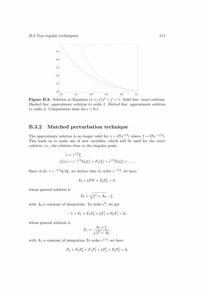
B.3 Non regular techniques 111
0.0 0.2 0.4 0.6 0.8 1.02.0
2.5
3.0
3.5
4.0
4.5
Figure B.3: Solution to Equation (x+ ϵf)f ′ + f = 1. Solid line: exact solution.Dashed line: approximate solution to ordre 1. Dotted line: approximate solutionto ordre 2. Computation done for ϵ = 0.1.
B.3.2 Matched perturbation technique
The approximate solution is no longer valid for x = O(ϵ1/2) where f = O(ϵ−1/2).This leads us to make use of new variables, which will be used for the innersolution, i.e., the solution close to the singular point:
x = ϵ1/2ξ,
fi(x) = ϵ−1/2F0(ξ) + F1(ξ) + ϵ1/2F2(ξ) + . . . .
Since d/dx = ϵ−1/2d/dξ, we deduce that to order ϵ−1/2, we have
F0 + ξF0′ + F0F′0 = 0,
whose general solution isF0 =
√ξ2 +A0 − ξ,
with A0 a constant of integration. To order ϵ0, we get
−1 + F1 + F1F′0 + ξF ′
1 + F0F′1 = 0,
whose general solution is
F1 = A1 + ξ√ξ2 +A0
,
with A1 a constant of integration To order ϵ1/2, we have
F2 + F2F′0 + F1F
′1 + ξF ′
2 + F0F′2 = 0,

112 B. Approximation
whose general solution is
F2 = −A21 − 2ξA1 + 2A2ξ
2 +A0 + 2A0A2
2 (ξ2 +A0)3/2 ,
with A2 a constant of integration.We now have to determine the constants of integration. Take a closer look at
the outer solution
f(x) = 1 + x
x+ ϵ
3x2 − 2x− 12x3 +O(ϵ2).
The change of variable x = ϵ1/2ξ shows that
• to order ϵ−1/2 and in the limit ξ → ∞, we have fϵ−1/2 ∼ ξ−1 while F0 ∼A0/(2ξ) hence A0 = 2 ;
• to order ϵ0 and in the limit ξ → ∞, we have fϵ0 ∼ 1 while F1 ∼ 1 hence weset A1 = 0 ;
• to order ϵ1/2 and in the limit ξ → ∞, we have fϵ1/2 ∼ 3/(2ξ) while F2 ∼A2/(ξ) hence A2 = 3/2.
The inner solution is
fi(ξ) = ϵ−1/2(√
ξ2 + 2 − ξ
)+ ξ√
ξ2 +A0+ ϵ1/2 3ξ2 + 8
2 (ξ2 + 2)3/2 ,
while the outer solution fe is given by (B.5). The composite solution is
f = fi + fe − fr,
with fr the matching value between fi and fe
fr = limξ→∞
fi = ϵ−1/2ξ−1 + 1 = 1x
+ 1.
We note that fe = fr. The solution is plotted on Fig. B.4. Note that reasonablygood agreement is obtained.

B.3 Non regular techniques 113
0.0 0.2 0.4 0.6 0.8 1.02.0
2.5
3.0
3.5
4.0
4.5
Figure B.4: Solution to Equation (x+ ϵf)f ′ + f = 1. Solid line: exact solution.Dashed line: approximate solution to ordre ϵ1/2. Dotted line: approximate solutionto ordre 1 using the stretched coordinate method. Computation done for ϵ = 0.1.


Bibliography
Bird, R.B., Armstrong, R.C. & Hassager, O. 1987 Dynamics of PolymericLiquids. New York: John Wiley & Sons.
Bird, R.B., Dai, G.C. & Yarusso, B.J. 1983 The rheology and flow of vis-coplastic materials. Rev. Chem. Eng. 1, 1–70.
Bluman, G.W. 1990 Invariant solutions for ordinary differential equations. SIAMJ. Appl. Math. 50, 1706–1715.
Boehler, J.P., ed. 1987 Applications of tensor functions in solid mechanics,International Centre for Mechanical Sciences, Courses and Lectures, vol. 292.New York: Springer Verlag.
Courant, R. & Friedrich, K.O. 1948 Supersonic Flow and Shock Waves. NewYork: Intersciences Publishers.
Dressler, L. 1983 Similarity Solutions of Nonlinear Partial Differential Equa-tions. Boston: Pitman.
Einstein, A. 1911 Berichtigung zu meiner Arbeit “Eine neue Bestimmung derMoleküldimensionen”. Annalen der Physik 34, 591–592.
Frankel, N.A. & Acrivos, A. 1967 On the viscosity of a concentrated suspen-sion of solid spheres. Chem. Eng. Sci. 22, 847–853.
Germain, P. 1973a La méthode des puissances virtuelles en mécanique des mi-lieux continus. Journal de Mécanique 12, 235–274.
Germain, P. 1973b The method of virtual power in continuum mechanics, Part2: Microstructure. SIAM J. Appl. Math. 25 (3), 556–575.
Huppert, H.E. 1982 Flow and instability of a viscous current down a slope.Nature 300, 427–429.
Hutter, K. & Jöhnk, K. 2004 Continuum Methods of Physical Modeling. Berlin:Springer.
Jones, C.W. 1953 On Reducible Non-Linear Differential Equations Occurring inMechanics,. Proc. R. Soc. London ser. A 217, 327–343.
115

116 BIBLIOGRAPHY
Lacey, A.A., Ockendon, J. R. & Tayler, A. B. 1982 "Waiting-Time" Solu-tions of a Nonlinear Diffusion Equation. SIAM J. Appl. Math. 42, 1252–1264.
LeVeque, R.J. 2002 Finite Volume Methods for Hyperbolic Problems. Cambridge:Cambridge University Press.
Minier, J.-P. & Peirano, E 2001 The pdf approach to turbulent polydispersedtwo-phase flows. Physics Reports 352 (1-3), 1–214.
Morrison, F.A. 2001 Understanding Rheology. New York: Oxford UniversityPress.
Oldroyd, J.G. 1950 On the formulation of rheological equations of state. Proc.R. Soc. London ser. A 200, 523–541.
Pope, S.B. 2000 Turbulent Flows. Cambridge: Cambridge University Press.
Tanner, R.I. 1988 Engineering Rheology. Oxford: Clarendon Press.
Truesdell, C. 1966 Six Lectures on Modern Natural Philosophy. New York:Springer Verlag.
Truesdell, C. 1974 The meaning of viscometry in fluid dynamics. Annu. Rev.Fluid Mech. 6, 111–147.
Zdunkowski, W. & Bott, A. 2003 Dynamics of the Atmosphere. Cambridge:Cambridge University Press.
Zheng, Q.-S. 1994 Theory of representations for tensor functions- A unified in-variant approach to constitutive equation. Appl. Mech. Rev. 47, 545–586.

Index
biharmonic, 4
characteristic, 71condition
boundary, 44Dirichlet, 44initial, 39, 44Lax, 76Neuman, 44Rankine-Hugoniot, 71
convection, 46, 50curl, 4curve
characteristic, 71
descriptionEulerian, 11Lagrangian, 11
diffusion, 47, 50, 85Dirac, 4divergence, 4
energyfree, 18kinetic, 26, 27total, 27
energy dissipation rate, 26, 28, 32equation
hyperbolic, 69Bernoulli, 27Buckley-Leverett, 76caractéristique, 46characteristic, 43, 70conservative, 31constitutive, 18continuity, 25elliptic, 41Euler-Darboux, 56Euler-Lagrange, 45
homogeneous, 41Huppert, 79hyperbolic, 41Navier-Stokes, 9non-conservative, 31parabolic, 41variational, 45wave, 52
équationde Fokker-Planck, 89
Bernoulli, 39Boussinesq, 56Burgers, 51characteristic, 67convection, 46diffusion, 47heat, 54Helmholtz, 56het, 47Klein-Gordon, 56Laplace, 54linear, 39nonlinear diffusion, 47Pascal, 39quasi-linear, 39
fading memory, 20fluid
inviscid, 27Newtonian, 8, 18, 32simple, 9, 17
formcharacteristic, 42
formecanonical, 41
Fourier transform, 4frequency, 52functional, 45
117

118 INDEX
gradient, 4Green, 47
harmonic, 4, 52heat, 27hodograph, 59
incompressible, 25integrale
first, 43invariance, 59, 62invariant, 21irrotational, 4isochoric, 25
jump, 30
Laplacian, 4law
Darcy, 54thermodynamics, 27
loide Fick, 85
materialhomogeneous, 20isotropic, 20
methodasymptotic, 62Green, 59hodograph, 59perturbations, 60
modelBingham, 33Maxwell, 35
node, 94, 97nombre
de Péclet, 90number
wave, 52
order, 39, 41
period, 52phase portrait, 93
pointcritical, 93focal, 94, 97singular, 93
pressure, 10, 17generalized, 27hydrostatic, 18mean, 18thermodynamic, 18
principleHamilton, 45variational, 45
problemGreen, 47Riemann, 73
relationdispersion, 52
rulel’Hôpital, 97plastic, 33
saddle, 94, 97self-similarity, 62separatrix, 97shock, 25, 42, 71similarity, 67singularity, 93solution
d’Alembert, 53similarity, 62, 67singular, 43
source, 69symmetry, 20system
hyperbolic, 69
tensorCauchy-Green, 13deviatoric strain, 21deviatoric stress, 10, 18, 21extra-stress, 10, 17gradient, 11Green-Lagrange, 13

INDEX 119
strain, 21strain rate, 15stress, 16, 21stretch, 13velocity gradient, 15
theoremCayley-Hamilton, 21Green-Ostrogradski, 4kinetic energy, 26Leibnitz, 23representation, 32Reynolds, 24transport, 23
transformLaplace, 49
transformationCole-Hopf, 51
variabledependant, 41independant, 41Riemann, 69
variable separation, 59velocity
group, 52wave, 52
viscoplastic, 33viscosity
dynamic, 8Newtonian, 8, 10Trouton, 8
vitessephase, 52
volumecontrol, 24material, 24
von Mises criterion, 34
wave, 52backward, 53compound, 76dynamic, 52forward, 53length, 52
progressive, 52rarefaction, 75shock, 75simple, 75
yield stress, 33