Lego Coriolis Vibrating GyroscopeLego Coriolis Vibrating Gyroscope 1 Introduction This document describes the design of a Coriolis vibrating gyroscope created out of Legos. The purpose

Lego Coriolis

Vibrating Gyroscope

by: Scott Gift2013

c© S.Gift

Scott GiftMasters of Engineering, Systems EngineeringBachelor of Science, Electrical Engineering

[email protected]@gmail.com

Lead Project EngineerPenn State University Applied Research Laboratory

Navigation Research and Development Center995 Newtown Road

Warminster, Pa 18974-2935Phone: 215-682-4016

Email: [email protected]

Lego Coriolis Vibrating Gyroscope

Contents

1 Introduction 5

2 Summary and Conclusion 7

3 Theory of Operation Overview 9

4 Detailed Analysis 134.1 Differential Equation of Motion . . . . . . . . . . . . . . . . . . . . . . . . . . . . . 15

4.1.1 Particular Solution . . . . . . . . . . . . . . . . . . . . . . . . . . . . . . . . 154.1.2 Resonant Frequency . . . . . . . . . . . . . . . . . . . . . . . . . . . . . . . 204.1.3 Homogeneous Solution . . . . . . . . . . . . . . . . . . . . . . . . . . . . . . 23

4.2 Coriolis Force . . . . . . . . . . . . . . . . . . . . . . . . . . . . . . . . . . . . . . . 274.3 Extracting the Rate Measurement . . . . . . . . . . . . . . . . . . . . . . . . . . . . 37

5 Mechanical System 39

6 Electromechanical System 43

7 Electrical System 47

8 Software 51

9 Testing Effort 53

10 Results 5710.1 Homogeneous Solution Results . . . . . . . . . . . . . . . . . . . . . . . . . . . . . . 5710.2 Bias-instability and ARW Results . . . . . . . . . . . . . . . . . . . . . . . . . . . . 6210.3 Scale Factor Results . . . . . . . . . . . . . . . . . . . . . . . . . . . . . . . . . . . 64

c© S.Gift 1


this page intentionally left blank

c© S.Gift 2


List of Figures

2.1 Lego Gyroscope on a Precision Rate Table . . . . . . . . . . . . . . . . . . . . . . . 72.2 Lego Gyroscope Output vs Input Rate . . . . . . . . . . . . . . . . . . . . . . . . . 8

3.1 Drive and Sense Axes . . . . . . . . . . . . . . . . . . . . . . . . . . . . . . . . . . . 93.2 (a) Mass oscillating along the drive axis; (b) mass under rotation also oscillates some

along the sense axis . . . . . . . . . . . . . . . . . . . . . . . . . . . . . . . . . . . 103.3 Drive Axis Setup . . . . . . . . . . . . . . . . . . . . . . . . . . . . . . . . . . . . . 103.4 Drive Axis Setup . . . . . . . . . . . . . . . . . . . . . . . . . . . . . . . . . . . . . 11

4.1 Mechanical Model of the System . . . . . . . . . . . . . . . . . . . . . . . . . . . . . 134.2 Relationship between the A and B coefficients . . . . . . . . . . . . . . . . . . . . . 184.3 Resonant Frequency Plots of Case 1 (blue) and Case 2 (red) . . . . . . . . . . . . . 214.4 Single Resonant Frequency Plot of Case 1 (blue) and Case 2 (red) . . . . . . . . . . 224.5 (a) Sense axis consists of a mass, spring, and damper; (b) the mass is moved to one

side and then “let go”; (c) after the ‘let go,” the mass oscillates with an exponentialdecay . . . . . . . . . . . . . . . . . . . . . . . . . . . . . . . . . . . . . . . . . . . 23

4.6 Typical response to a homogeneous equation with complex roots; the mass is “letgo” at 2 sec . . . . . . . . . . . . . . . . . . . . . . . . . . . . . . . . . . . . . . . . 24

4.7 2D representation of two coordinate frames . . . . . . . . . . . . . . . . . . . . . . . 274.8 Rate Measurement Block Diagram . . . . . . . . . . . . . . . . . . . . . . . . . . . 37

5.1 Mechanical Overview . . . . . . . . . . . . . . . . . . . . . . . . . . . . . . . . . . . 395.2 Mechanical Drive Axis . . . . . . . . . . . . . . . . . . . . . . . . . . . . . . . . . . 405.3 M1 Photo . . . . . . . . . . . . . . . . . . . . . . . . . . . . . . . . . . . . . . . . . 405.4 Mechanical Sense Axis . . . . . . . . . . . . . . . . . . . . . . . . . . . . . . . . . . 415.5 Rubber Band Photo . . . . . . . . . . . . . . . . . . . . . . . . . . . . . . . . . . . 415.6 Mechanical Photo . . . . . . . . . . . . . . . . . . . . . . . . . . . . . . . . . . . . . 42

6.1 Drive Axis Setup . . . . . . . . . . . . . . . . . . . . . . . . . . . . . . . . . . . . . 436.2 Drive Axis Configuration . . . . . . . . . . . . . . . . . . . . . . . . . . . . . . . . . 446.3 Axis Pickups . . . . . . . . . . . . . . . . . . . . . . . . . . . . . . . . . . . . . . . 446.4 Side view of Potentiometer . . . . . . . . . . . . . . . . . . . . . . . . . . . . . . . . 45

7.1 Electrical Block Diagram . . . . . . . . . . . . . . . . . . . . . . . . . . . . . . . . . 47

c© S.Gift 3


7.2 Electrical Schematic . . . . . . . . . . . . . . . . . . . . . . . . . . . . . . . . . . . 487.3 Electrical Circuit Photo . . . . . . . . . . . . . . . . . . . . . . . . . . . . . . . . . 487.4 Ohms to Volts . . . . . . . . . . . . . . . . . . . . . . . . . . . . . . . . . . . . . . . 49

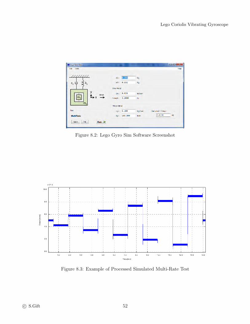
8.1 Arduino ComPortScope Software Screenshot . . . . . . . . . . . . . . . . . . . . . . 518.2 Lego Gyro Sim Software Screenshot . . . . . . . . . . . . . . . . . . . . . . . . . . . 528.3 Example of Processed Simulated Multi-Rate Test . . . . . . . . . . . . . . . . . . . 52

9.1 At the House on the Drill . . . . . . . . . . . . . . . . . . . . . . . . . . . . . . . . 549.2 Test 1001 Time Data . . . . . . . . . . . . . . . . . . . . . . . . . . . . . . . . . . . 549.3 On the Rate Table . . . . . . . . . . . . . . . . . . . . . . . . . . . . . . . . . . . . 559.4 Test 1003 Time Data . . . . . . . . . . . . . . . . . . . . . . . . . . . . . . . . . . . 55

10.1 Two dimensional plot of residuals from the homogeneous solution fit for Test-A . . . 6010.2 Two dimensional plot of residuals from the homogeneous solution fit for Test-B . . . 6010.3 Measured data from the Lego gyroscope (blue) and best homogeneous solution fit

(red) for Test-A . . . . . . . . . . . . . . . . . . . . . . . . . . . . . . . . . . . . . . 6110.4 Measured data from the Lego gyroscope (blue) and best homogeneous solution fit

(red) for Test-B . . . . . . . . . . . . . . . . . . . . . . . . . . . . . . . . . . . . . . 6110.5 Data verses Time . . . . . . . . . . . . . . . . . . . . . . . . . . . . . . . . . . . . . 6310.6 Allan-Deviation . . . . . . . . . . . . . . . . . . . . . . . . . . . . . . . . . . . . . . 6310.7 PSD Plot . . . . . . . . . . . . . . . . . . . . . . . . . . . . . . . . . . . . . . . . . 6310.8 Lego Gyroscope Output vs Input Rate . . . . . . . . . . . . . . . . . . . . . . . . . 64

c© S.Gift 4


1

Introduction

This document describes the design of a Coriolis vibrating gyroscope created out of Legos. Thepurpose of this work was two fold: to build a working gyroscope and to understand the math in-volved with such an endeavor. A gyroscope is a device that outputs (senses) a change in angle.This change in angle over time is referred to as rate. The basic principle of operation of a Coriolisvibrating gyroscope is that an object vibrating along a direction will want to stay vibrating in thatsame direction even under rotation. When the device undergoes a rotation, some of the vibration istransferred to an orthogonal direction. The amount that is transferred along the orthogonal direc-tion is proportional to the rotational rate. Using this principal, a device can be created to measurethe amount of rotational rate being experienced. These type of devices are referred to as gyroscopes.

The Lego gyroscope described within this document was a at-home research project. Initial testingof the Lego gyroscope consisted of mounting it on-top of a cordless drill. Follow-on testing wasconducted at the Navigation Research and Development Center (NRDC) in Warminster Pennsylva-nia. It is from these tests that the data is presented within this document. It is noted that testingwas limited and primarily used to verify that the Lego gyroscope worked as a gyroscope. Also, noattempt was made to optimize the design for performance gains.

The Lego gyroscope did measure rate as the next section describes. After this section is detailedanalysis on the mathematics used to describe the gyroscope. This is followed by a description ofa software simulation designed to verify the system. An overview of the Lego gyroscope is alsopresented but it is noted that this section is only a overview and not intended to be detailed enoughto build a replica. The document finishes with details of the testing effort with analyzed data.

c© S.Gift 5



c© S.Gift 6


2

Summary and Conclusion

Testing was conducted at the Navigation Research and Development Center (NRDC) in Warmin-ster Pennsylvania on a precision rate table. The purpose of this testing was to prove that the Legogyroscope did indeed function as a gyroscope. This testing was conducted in May of 2013 over aperiod of days. Figure 2.1 shows the Lego gyroscope mounted on a precision rate table.

(a) (b)

Figure 2.1: Lego Gyroscope on a Precision Rate Table

c© S.Gift 7


Figure 2.2: Lego Gyroscope Output vs Input Rate

The precision rate table was rotated at ±100 deg/sec, ±150 deg/sec, and ±190 deg/sec. Data wasrecorded throughout the test effort. From the data collected, a linear fit was applied to the gyrooutput versus the input rate. This fit is show in Figure 2.2. The Lego gyroscope scale factor wasdetermined to be 33333 deg/sec/output. The Lego gyroscope in-run bias was determined to be -143deg/sec. The fit also shows a large scale factor non-linearity which is expected because of the Legodesign using rubber bands for the springs. The bias-instability was also calculated from anothertest and determined to be about 11370 deg/hr. Angle Random Walk (ARW) was calculated to be1063 deg/

√hr.

The goals of this project were fulfilled completely. The gyroscope was tested and did measure inputrate; the Lego contraption was a gyroscope. The other goal was met through the existence of thisdocument, specifically the analytical section. Going ahead, the author has no plans to improveon the Lego gyroscope design. In fact, many of the parts will probably be reclaimed for otherendeavors. Further refining of the device could be accomplished with many simple improvements,but these are left to the reader to further investigate.

c© S.Gift 8


3

Theory of Operation Overview

A gyroscope is a device that outputs (senses) a change in angle. This change in angle over timeis referred to as rate. The basic principle of operation of a Coriolis vibrating gyroscope is that anobject vibrating along a direction will want to stay vibrating in that same direction even underrotation. This is referred to as staying inertial stable. When the device undergoes a rotation, someof the vibration is transferred to an orthogonal axis through the Coriolis effect. The amount thatis transferred is proportional to the rotational rate.

More specifically, the Coriolis effect describes mathematically what happens when an object is mov-ing in a rotating frame. The stationary frame of reference can be considered the inertial frame.When an object rotates, its coordinate frame rotates with respect to the inertial frame. This intro-duces a special force referred to as a fictitious force. This force is what “moves” some of the motionto the other axis.

Figure 3.1 depicts the basic principle of the device. There is a mass that can move in two directions:along the drive axis and the sense axis. An oscillation is driven along the drive axis of the device.This moves the mass back and forth at a specified frequency.

Figure 3.1: Drive and Sense Axes

c© S.Gift 9


When the oscillating mass is rotated, some of the oscillation will transfer to the other axis. Theamount of oscillation transferred is proportional to the angular rate as shown in figure 3.2.

(a) (b)

Figure 3.2: (a) Mass oscillating along the drive axis; (b) mass under rotation also oscillates somealong the sense axis

For the Lego gyroscope developed, a direct linkage from the motor to the mass was used to createthe oscillation along the drive axis. This design is shown in figure 3.3. A Lego motor was connecteddirectly to a Lego gear. One side of a Lego shaft was connected to the edge of the gear and theother side to the mass. In this configuration, the constantly rotating motor was used to make themass oscillate back and forth.

Figure 3.3: Drive Axis Setup

c© S.Gift 10


The sense axis was created using rubber bands and placing the entire assembly on wheels to lowerfriction (damping). The rubber bands acted as springs. To maximize the gyroscope potential, thesense axis was tuned to resonate at the same frequency as the oscillating mass. Figure 3.4 showsa typical mass, spring, damper system. This type of system creates a differential equation. Theanalysis section of this document describes this in more detail.


The motor oscillated the mass back and forth at a constant frequency along the drive axis. Thesense axis was tuned close to the frequency of the drive axis. Then when a rotation rate was applied,the sense axis also oscillated. The magnitude of oscillation was proportional to the magnitude ofthe input rate and measured by the supporting electronics.

c© S.Gift 11



c© S.Gift 12


4

Detailed Analysis

This chapter describes how the Lego Coriolis vibrating gyroscope operates mathematically. Thefollowing is an overview of the system. The next section describes in detail the differential equationused for a typical mass, damper, and spring system with a sinusoidal forcing function. A closedform solution is presented. A derivation of the Coriolis force is presented next. This is followed bya short description on extracting the rate from the measurement.

The mechanical system for the Lego gyroscope is shown in figure 4.1. The mass M1 is sinusoidallyvibrated along the x-axis by a motor. This is considered the drive axis. Masses M1 and M2 canfreely move along the y-axis. This is considered the sense axis. When a rotation is applied aboutthe z-axis (out of the page), then some of the vibration will be transferred to the y-axis.

Figure 4.1: Mechanical Model of the System

c© S.Gift 13


The motion along the x-axis can be described in the following equations. For this Lego gyroscope,Dx is approximate 20 mm.

x = Dxcos(ωt)

x = −ωDxsin(ωt)

The Coriolis force is important to the Lego gyroscope because it is this fictitious-force that allowsthe sense axis to pickup a portion of the motion along the drive axis when the Lego gyroscope isrotating. The Coriolis force with a constant input rate of Ωz will be the following.

Coriolis force = −2M1xΩz

The equation of motion along the y-axis will be a spring, mass, and damper system with the Coriolisforce as shown in equation 4.1.

(M1 +M2) y + cyy + ky = 2ωM1DxΩzsin(ωt) (4.1)

The particular solution to the differential is shown in equation 4.2. The next section details thesteps to derive the this solution.

yp = 2ωM1DxΩzρysin(ωt− αy) (4.2)

ρy =1√

(ky − (M1 +M2)ω2)2 + (cy ω)2

αy = tan−1

(cy ω

ky − (M1 +M2)ω2

)

The resonant frequency, f0, of the system is then:

ω0 =

√(ky

(M1 +M2)− cy2

2(M1 +M2)2

)(4.3)

f0 =ω0

2π(4.4)

c© S.Gift 14


4.1 Differential Equation of Motion

The mechanical system described in figure 4.1 consists of a mass, a damper, and a spring. Theequation that describes this motions is shown in equation 4.5.

my + cy + ky = F (4.5)

m is the mass, c is the damping coefficient, k is the spring coefficient, and F is the forcing func-tion. Lego gyroscope’s motor oscillates the mass at a constant frequency and is simply modeled asF0cos(ωt+ θ). The full differential equation is then shown to be:

my + cy + ky = F0cos(ωt+ θ) (4.6)

4.1.1 Particular Solution

The particular solution to this problem will have the form:

yp = Acos(ωt+ θ) +Bsin(ωt+ θ) (4.7)

To solve for A and B, the derivatives of the particular solution (yp, yp, and yp) are calculated andplugged back into the original equation. This then reduces down to equations 4.8 and 4.9 in theform of two equations with two unknowns.

Calculating the derivative of the particular solution yields:

yp = Acos(ωt+ θ) +Bsin(ωt+ θ)

yp = −Aωsin(ωt+ θ) +Bωcos(ωt+ θ)

yp = −Aω2cos(ωt+ θ)−Bω2sin(ωt+ θ)

c© S.Gift 15


Substituting the particular solution into equation 4.6 yields:

−mAω2cos(α)−mBω2sin(α)−cAωsin(α) + cBωcos(α)+

kAcos(α) +Bksin(α) = F0cos(α) where α = ωt+ θ

After collecting the terms and rearranging the equation becomes:

(−mAω2 + cBω + kA

)cos(α) = F0cos(α)(

−mBω2 − cAω + kB)sin(α) = 0

This reduces to:

(−mAω2 + cBω + kA

)= F0 (4.8)(

−mBω2 − cAω + kB)

= 0 (4.9)

Shown in in matrix form: [(k −mω2) c ω−c ω (k −mω2)

] [AB

]=

[F0

0

](4.10)

To get the solution to the coefficients A and B, each side of equation 4.10 is multiplied by theinverse of the model coefficient terms matrix. This changes the equation to:[

AB

]=

[(k −mω2) c ω−c ω (k −mω2)

]−1 [F0

0

](4.11)

c© S.Gift 16


The general form of 2x2 matrix and inverse is:

A =

[a bc d

]A−1 =

1

det(A)

[d −b−c a

]=

1

ad− bc

[d −b−c a

]Inverse of the model coefficient matrix is then:[

(k −mω2) c ω−c ω (k −mω2)

]−1

=1

(k −mω2)(k −mω2) + (c ω)(c ω)

[(k −mω2) −c ω

c ω (k −mω2)

]

Equation 4.11 has a zero in the matrix to the right which can be used to make the solution simpler.This simplification is:

[AB

]=

[d −b−c a

] [F0

0

][AB

]=

[d−cF0

]

The A and B coefficients are then solved to be:

A =(k −mω2)F0

(k −mω2)2 + (c ω)2(4.12)

B =(c ω)F0

(k −mω2)2 + (c ω)2(4.13)

c© S.Gift 17


Notice that in equations 4.12 and 4.13, the A and B coefficients have the same denominator. Alsonotice that the numerators are terms from the denominator. These terms can then be expressed interms of a sin and cos as shown in the triangle diagram, Figure 4.2, and following equations [3]:

k −mω2

c ω

α

Figure 4.2: Relationship between the A and B coefficients

hypotenuse =√

(k −mω2)2 + (c ω)2

cos(α) =k −mω2√

(k −mω2)2 + (c ω)2

sin(α) =c ω2√

(k −mω2)2 + (c ω)2

Using a new term ρ, coefficients A and B can be simply expressed as:

ρ =1√

(k −mω2)2 + (c ω)2

A = ρF0cos(α) (4.14)

B = ρF0sin(α) (4.15)

c© S.Gift 18


The A and B coefficients, equations 4.14 and 4.15, then get plugged back into the particular solution:

yp = Acos(ωt+ θ) +Bsin(ωt+ θ)

= ρF0cos(α)cos(ωt+ θ) + ρF0sin(α)sin(ωt+ θ)

Using the trigonometric identity cos(x1 − x2) = cos(x1)cos(x2) + sin(x1)sin(x2), the analyticalsolution to the differential problem is shown to be:

yp = ρF0cos(ωt+ θ − α) (4.16)

ρ =1√

(k −mω2)2 + (c ω)2(4.17)

α = tan−1

(c ω

k −mω2

)(4.18)

c© S.Gift 19


4.1.2 Resonant Frequency

The resonant frequency is the place in hertz that the system will give the maximum excitation. Inthe case for this given system, it is the place of maximum displacement. The resonant frequency forequations 4.17 and 4.18 can be calculated analytically by finding the minimum of ρ’s denominator.This will make the amplitude of the sinusoids the highest. This is accomplished by finding wherethe denominator’s derivative is zero. The solution is to determine at what ω the system resonate.This is referred to as ω0.

g(ω0) = (k −mω02)2 + (c ω0)2

= k2 − 2kmω20 +m2ω4

0 + c2ω20

g(ω0) = −4kmω0 + 4m2ω03 + 2c2ω0

the minimum is when g(ω0) = 0

0 = 4m2ω03 +

(2c2 − 4km

)ω0

0 = ω03 +

(2c2

4m2− 4km

4m2

)ω0

0 = ω03 +

(c2

2m2− k

m

)ω0

ω03 = −

(c2

2m2− k

m

)ω0

ω02 =

(k

m− c2

2m2

)ω0 =

√(k

m− c2

2m2

)

Since ω0 = 2πf0, the resonant frequency in hertz (hz) can be calculated by:

f0 =

(1

2π

)√(k

m− c2

2m2

)(4.19)

c© S.Gift 20


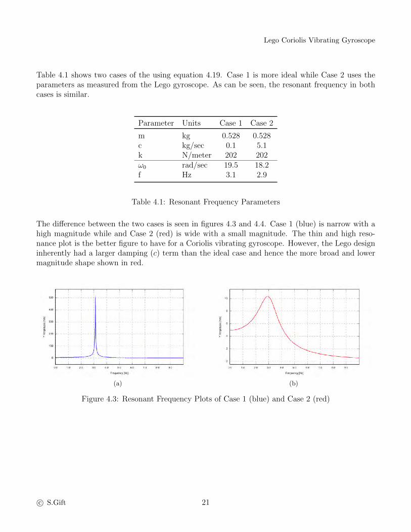
Table 4.1 shows two cases of the using equation 4.19. Case 1 is more ideal while Case 2 uses theparameters as measured from the Lego gyroscope. As can be seen, the resonant frequency in bothcases is similar.

Parameter Units Case 1 Case 2

m kg 0.528 0.528c kg/sec 0.1 5.1k N/meter 202 202ω0 rad/sec 19.5 18.2f Hz 3.1 2.9

Table 4.1: Resonant Frequency Parameters

The difference between the two cases is seen in figures 4.3 and 4.4. Case 1 (blue) is narrow with ahigh magnitude while and Case 2 (red) is wide with a small magnitude. The thin and high reso-nance plot is the better figure to have for a Coriolis vibrating gyroscope. However, the Lego designinherently had a larger damping (c) term than the ideal case and hence the more broad and lowermagnitude shape shown in red.

(a) (b)

Figure 4.3: Resonant Frequency Plots of Case 1 (blue) and Case 2 (red)

c© S.Gift 21


Figure 4.4: Single Resonant Frequency Plot of Case 1 (blue) and Case 2 (red)

c© S.Gift 22


4.1.3 Homogeneous Solution

The homogeneous solution to the differential equation along the sense axis is useful in determin-ing the system’s parameters. The mass (m) of the system for the Lego gyroscope was determinedby measurement with a scale. The spring (k) and damper (c) terms were determined by physi-cally moving the Lego gyroscope’s mass to the left or right along the sense axis then letting goas illustrated in figure 4.5. When “let go,” the system would oscillate with an exponential decay.This type of response is expected and shown by the solution to the homogeneous equation, figure 4.6.

(a) (b)

(c)

Figure 4.5: (a) Sense axis consists of a mass, spring, and damper; (b) the mass is moved to one sideand then “let go”; (c) after the ‘let go,” the mass oscillates with an exponential decay

c© S.Gift 23


Figure 4.6: Typical response to a homogeneous equation with complex roots; the mass is “let go”at 2 sec

The following equation is the characteristic equation to the homogeneous solution (yh).

mr2 + cr + k = 0

The roots of the characteristic equation are:

r =−c±

√c2 − 4mk

2m

c© S.Gift 24


There exist three possible solution types to the homogeneous equation. The solutions are dependingon the types of the roots: distinct real roots, repeated roots, or complex roots.

Distinct Real Roots (c2 > 4mk)

r1 =−c+

√c2 − 4mk

2m

r2 =−c−

√c2 − 4mk

2m

yh = C1er1t + C2e

r2t

Repeated Roots (c2 == 4mk)

r1, r2 =c

2m

yh = (C1 + C2t) e−c2m

t

Complex roots (c2 < 4mk)

r =−c2m±√

4mk − c2

2mi (4.20)

yh = e−c2m

t

[C1cos

(√4mk − c2

2mt

)+ C2sin

(√4mk − c2

2mt

)](4.21)

c© S.Gift 25



c© S.Gift 26


4.2 Coriolis Force

This section mathematically derives the fictitious Coriolis force and is based on the paper Equationsof Motion For Rotating Frames by Nick Saluzzi [1]. The Coriolis force is important to the Legogyroscope because it is this fictitious-force that allows the sense axis to pickup a portion of themotion along the drive axis when the Lego gyroscope is rotating. This section concludes with thegeneral form for the motion equation with respect to a rotating frame about the z-axis. This isshown in equation 4.22 with a more specific equation shown in equation 4.23.

Figure 4.7 depicts a two dimensional scenario of two independent coordinate frames. P is the loca-tion of an arbitrary object with mass having three components: x, y, z (note, only two dimensionsare shown in the figure). Vector VA represents the position of the object in coordinate frame A.Vector VB represents the position of the object in coordinate frame B. Vector VAB represents theposition of coordinate B in coordinate frame A.

A

u2

B

u1

VAB

VB

VA

P

Figure 4.7: 2D representation of two coordinate frames

It can be seen that Vector VA is the summation of VAB and VB.

VA = VAB + VB

This equation can be represented as the summation of the vector components:

VA,xVA,yVA,z

=

VAB,xVAB,yVAB,z

+

VB,xVB,yVB,z

c© S.Gift 27


This can be broken down further:

VB = VB,x

100

+ VB,y

010

+ VB,z

001

Vector VB is can be rewritten as the sum of unit vectors: ux, uy, and uz.

ux =

100

, uy =

010

, uz =

001

Then this can be put into sigma notation:

VB = VB,xux + VB,yuy + VB,zuz

=∑k

(VB,kuk)

where k = x, y, z

Equations are typically written as a summation of forces. A force consists of a mass and an accel-eration. This infers that the vector equations need to be expressed in terms of acceleration vectors.

VA =d2

dt2VA

The derivatives are expressed as:

VA = VAB +∑k

(VB,kuk)

VA = VAB +∑k

(VB,kuk

)+∑k

(VB,kuk)

VA = VAB +∑k

(VB,kuk

)+∑k

(VB,kuk

)+∑k

(VB,kuk

)+∑k

(VB,kuk)

= VAB + VB,k + 2∑k

(VB,kuk

)+∑k

(VB,kuk)

c© S.Gift 28


For the single axis gyroscope, there is a rotation about the z-axis as specified by Rz(θ):

Rz(θ) =

cos(θ) −sin(θ) 0sin(θ) cos(θ) 0

0 0 1

This rotation can be applied to the unit vectors:

ux = Rz(θ)ux =


0 0 1

100

=

cos(θ)sin(θ)0

uy = Rz(θ)uy =


0 0 1

010

=

−sin(θ)cos(θ)

0

uz = Rz(θ)uz =


0 0 1

001

=

001

The first derivatives (rate) of the rotated unit vectors are:

ux =

−θsin(θ)

θcos(θ)0

uy =

−θcos(θ)−θsin(θ)0

uz =

000

c© S.Gift 29


The second derivatives (acceleration) of the rotated unit vectors are:

ux =

−θsin(θ)− θ2cos(θ)

θcos(θ)− θ2sin(θ)0

uy =

−θcos(θ) + θ2sin(θ)

−θsin(θ)− θ2cos(θ)0

uz =

000

The first derivative can expressed as:

ux = θuy

uy = −θuxuz = [0, 0, 0]T

The second derivative similarly be can expressed as:

ux = θuy − θ2ux

uy = −θux − θ2uy

uz = [0, 0, 0]T

Using the following substitution:

ux

θ= uy

−uy

θ= −ux

c© S.Gift 30


The second derivative can now be expressed as:

ux = θuy + θuy

uy = −θux − θuxuz = [0, 0, 0]T

The rate vector is expressed as:

Ω =

00

θ

The cross product of Ω and ux is:

Ω× ux =

∣∣∣∣∣∣ux uy uz0 0 θ

cos(θ) sin(θ) 0

∣∣∣∣∣∣=

−θsin(θ)

θcos(θ)0

= ux

Similarly:

Ω× uy =

∣∣∣∣∣∣ux uy uz0 0 θ

−sin(θ) cos(θ) 0

∣∣∣∣∣∣=

−θcos(θ)−θsin(θ)0

= uy

c© S.Gift 31


The derivatives of the cross products are:

d

dt(Ω× ux) = Ω× ux + Ω× ux

= Ω× ux + Ω× (Ω× ux)

d

dt(Ω× uy) = Ω× uy + Ω× uy

= Ω× uy + Ω× (Ω× uy)

Ω× ux =

∣∣∣∣∣∣ux uy uz0 0 θ

cos(θ) sin(θ) 0

∣∣∣∣∣∣ =

−θsin(θ)

θcos(θ)0

= θuy

Ω× (Ω× ux) = Ω×

−θsin(θ)

θcos(θ)0

=

∣∣∣∣∣∣ux uy uz0 0 θ

−θsin(θ) θcos(θ) 0

∣∣∣∣∣∣ =

−θ2cos(θ)

−θ2sin(θ)0

= θuy

d

dt(Ω× ux) = Ω× ux + Ω× (Ω× ux)

= θuy + θuy

= ux

d

dt(Ω× uy) = Ω× uy + Ω× (Ω× uy)

= −θux − θux= uy

c© S.Gift 32


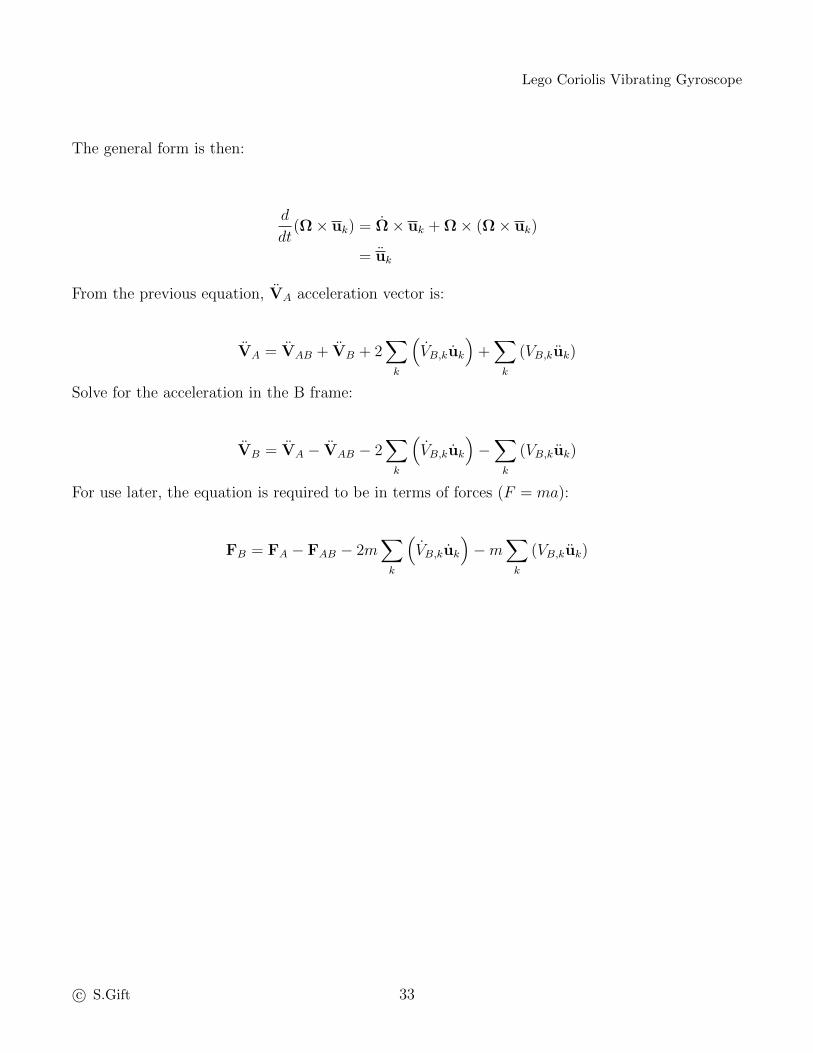
The general form is then:

d

dt(Ω× uk) = Ω× uk + Ω× (Ω× uk)

= uk

From the previous equation, VA acceleration vector is:

VA = VAB + VB + 2∑k

(VB,kuk

)+∑k

(VB,kuk)

Solve for the acceleration in the B frame:

VB = VA − VAB − 2∑k

(VB,kuk

)−∑k

(VB,kuk)

For use later, the equation is required to be in terms of forces (F = ma):

FB = FA − FAB − 2m∑k

(VB,kuk

)−m

∑k

(VB,kuk)

c© S.Gift 33


Before continuing, an identity needs to be proved,∑

k [Ak (Ω× uk)] = Ω × A, where A is somearbitrary vector.

Ω×A reduces to:

Ω×A =

∣∣∣∣∣∣x y z

0 0 θAx Ay Az

∣∣∣∣∣∣ =

∣∣∣∣∣∣−θAyθAx

0

∣∣∣∣∣∣∑k [Ak (Ω× uk)] reduces to:

∑k

[Ak (Ω× uk)] = Ax (Ω× ux) + Ay (Ω× uy) + Az (Ω× uz)

= Ax

∣∣∣∣∣∣x y z

0 0 θ1 0 0

∣∣∣∣∣∣+ Ay

∣∣∣∣∣∣x y z

0 0 θ0 1 0

∣∣∣∣∣∣+ Az

∣∣∣∣∣∣x y z

0 0 θ0 0 1

∣∣∣∣∣∣= Ax

∣∣∣∣∣∣0

θ0

∣∣∣∣∣∣+ Ay

∣∣∣∣∣∣−θ00

∣∣∣∣∣∣+ Az

∣∣∣∣∣∣000

∣∣∣∣∣∣=

∣∣∣∣∣∣0

θAx0

∣∣∣∣∣∣+

∣∣∣∣∣∣−θAy

00

∣∣∣∣∣∣=

∣∣∣∣∣∣−θAyθAx

0

∣∣∣∣∣∣By inspection it can be seen that the two equations are equal. Taking the force equation and ro-tating frame B about the z-axis:

FB = FA − FAB − 2m∑k

(VB,kuk

)−m

∑k

(VB,kuk

)= FA − FAB − 2m

∑k

[VB,k (Ω× uk)

]−m

∑k

[VB,k

(Ω× uk + Ω× (Ω× uk)

)]

c© S.Gift 34


Making some substitutions, rB = VB and vB = VB, gives the general form:

FB = FA − FAB − 2m (Ω× vB)−m(Ω× rB

)−m (Ω× (Ω× rB)) (4.22)

FB Force observed in frame BFA Force exerted on the mass in the inertial frame AFAB Force observed in frame B due to the translation of frame B in the inertial frame Am: Mass of the bodyrB Displacement of the mass in frame BVB Velocity of the mass in frame B

Ω Rotation rate about the z-axis,[0, 0, θ

]T2m (Ω× vB) Coriolis fictitious force observed in frame B

m(Ω× rB

)Euler fictitious force observed in frame B

m (Ω× (Ω× rB)) Centrifugal fictitious force observed in frame B

For the rotating frame:

Ω× vB =

∣∣∣∣∣∣−vB,yθvB,xθ

0

∣∣∣∣∣∣Ω× rB =

∣∣∣∣∣∣−rB,yθrB,xθ

0

∣∣∣∣∣∣Ω× (Ω× rB) = Ω×

∣∣∣∣∣∣−rB,yθrB,xθ

0

∣∣∣∣∣∣ =

∣∣∣∣∣∣−rB,xθ2

−rB,yθ2

0

∣∣∣∣∣∣Substituting into equation 4.22:

FB,x = FA,x − FAB,x + 2mvB,yθ +mrB,yθ +mrB,xθ2

FB,y = FA,y − FAB,y − 2mvB,xθ −mrB,xθ +mrB,yθ2

FB,z = FA,z − FAB,z

c© S.Gift 35


If θ(t) is the constant rotation, this can be rewritten a function of time with a phase offset (φ(t)):

θ(t) = Ωz t+ φ(t)

θ(t) = Ωz + φ(t)

θ(t) = φ(t)

And[θ(t)

]2

is:

[θ(t)

]2

=(

Ωz + φ(t))(

Ωz + φ(t))

= Ωz2 + 2Ωzφ(t) +

(φ(t)

)2

Then substituting into the individual force equations:

FB,x = FA,x − FAB,x + 2mvB,yΩz + 2mvB,yθ(t) +mrB,yφ(t) +mrB,xΩz2 + 2mrB,xΩz θ(t) +mrB,x

(φ(t)

)2

FB,y = FA,y − FAB,y − 2mvB,xΩz + 2mvB,xθ(t)−mrB,xφ(t) +mrB,yΩz2 + 2mrB,yΩz θ(t) +mrB,y

(φ(t)

)2

FB,z = FA,z − FAB,z

If the phase angle (θ) is constant, then the derivative are zero, θ = θ = 0. The equations simplify to:

FB,x = FA,x − FAB,x + 2mvB,yΩz +mrB,xΩz2

FB,y = FA,y − FAB,y − 2mvB,xΩz +mrB,yΩz2

FB,z = FA,z − FAB,z(4.23)

c© S.Gift 36


4.3 Extracting the Rate Measurement

There are two channels of data from the gyro: drive and sense. The drive signal is read in onchannel 0 (A0). The sense signal is read in on channel 1 (A1). Both channels are run through abandpass filter set to 2 to 5 Hz. These signals are then mixed and low-pass filters to get the in-phaseresponse. The in-phase signal (I) is the gyroscope output. Figure 4.8 shows this block diagram.

Figure 4.8: Rate Measurement Block Diagram

c© S.Gift 37



c© S.Gift 38


5

Mechanical System

The entire gyroscope was constructed out of Lego building blocks except for a few exceptions. Awooden base was added to provide mounting wholes to attached the gyroscope to the precision ratetable. The weight for M1 was achieved with stainless steel bolts. Lego wheels were used to lowerthe friction of the moving parts. There are two moving parts: M1 and M2 as show in figure 5.1. M1

can only move along the drive axis and M2 can only move along the sense axis. Table 5.1 lists themasses. Figure 5.6 is a photo of one of the entire system. Figure 5.2 depicts the drive axis (x-axis).Figure 5.3 is a photo of M1. The bolts were secured using a hot glue gun.

Figure 5.1: Mechanical Overview

c© S.Gift 39


Parameter Units Measurement

M1 kg 0.296M2 kg 0.232M1 +M2 kg 0.528

Table 5.1: Mechanical Masses

Figure 5.2: Mechanical Drive Axis

Figure 5.3: M1 Photo

c© S.Gift 40


The sense axis (y-axis) was created using rubber bands and placing the sense assembly on wheels.The rubber bands allowed the sense axis to have a resonant frequency at the frequency of the driveaxis. Figure 5.4 depicts the sense axis. Figure 5.5 is a photo of one of the rubber bands. Figure 5.6is a photograph of the entire Lego gyroscope with the axis labeled.

Figure 5.4: Mechanical Sense Axis

Figure 5.5: Rubber Band Photo

c© S.Gift 41


Figure 5.6: Mechanical Photo

c© S.Gift 42


6

Electromechanical System

For the Lego gyroscope, a direct linkage from the motor to the mass was used to create the oscilla-tion along the drive axis. This design is shown in figure 6.1. A Lego motor was connected directlyto a Lego gear. One side of a Lego shaft was connected to the edge of the gear and the other side tothe mass. In this configuration, the constantly rotating motor was used to make the mass oscillateback and forth. The frequency of the oscillition was chosen to be at the resonant frequency of thesense axis. The Lego pieces connecting the shaft to the gear and to the mass did require a specialnon-Lego pin and glue to keep from separating over time. Figure 6.2 is a photograph of the drivemechanism.


c© S.Gift 43


Figure 6.2: Drive Axis Configuration

A potentiometer was used to convert the mechanical motion to and electrical signal. Two 20KΩpotentiometers were used on each axis. Figure 6.3 shows the configuration of each axis. The linearmotion of the bottom piece rotates the gear. This rotation is measured as a change in the resistance.Figure 6.4 show a side view of the potentiometer.

Figure 6.3: Axis Pickups

c© S.Gift 44


Figure 6.4: Side view of Potentiometer

A test was conducted to see what the change in resistance of potentiometer would be starting atdifferent center ohms. The travel distance was ±20 millimeters for the drive direction (x-axis) and±25 millimeters for the sense direction (y-axis). Table 6.1 contains this data. The conversion factorwas then calculated from this data. For simplicity, a single conversion factor of 22 Ω per millimeterwas selected.

The conversion factor =Ω Range

Distance Traveled

CenterΩ

X RangeΩ

Y RangeΩ

XΩ/mm

YΩ/mm

1000 566, 1395 388, 1593 21 242000 1670, 2480 1410, 2660 20 2510000 9450, 10250 9430, 10650 20 2415000 14540, 15410 14420, 15640 22 24

Table 6.1: Potentiometer Values Across the Travel Range

c© S.Gift 45



c© S.Gift 46


7

Electrical System

The electronics for the gyroscope was a simple design as seen in figure 7.1. The motor moves thedrive axis (x-axis). The distance traveled is converted to a voltage by way of a voltage divider. Ifthe gyro is in a rotating frame about the z-axis, the Coriolis force will move the sense axis (y-axis).This motion is also converted to a voltage. Both voltages will then be sampled and read into themicrocontroller by way of two 12-bit analog-to-digital (A/D) converter. The microcontroller usedwas an Arduino Due with channels A0 and A1 used for the conversion. The data was then sent toa computer for processing over a RS232 serial link. Figure 7.2 shows the electric schematic for thesystem. Figure 7.3 is the photograph of the circuit.

Figure 7.1: Electrical Block Diagram

c© S.Gift 47


Figure 7.2: Electrical Schematic

Figure 7.3: Electrical Circuit Photo

c© S.Gift 48


Figure 7.4 shows the circuit to convert ohms to volts so that it can be read into the Arduino’s A/D.The A/D’s range is 0 to 3.3 volts.

Figure 7.4: Ohms to Volts

The following equations describe the circuit.

VS = I(R +RP ) and VA = I RP

VS =VARP

(R +RP )

VA =VS RP

(R +RP )

Some of the parameters are know:

R = 1000Ω(selected based on inventory)

RP = RB + ∆R

RB is the potentiometer bias

∆R is the potentiometer range of motion about the bias

∆R = ±550Ω

(22Ω

mm@ ± 25mm

)

c© S.Gift 49


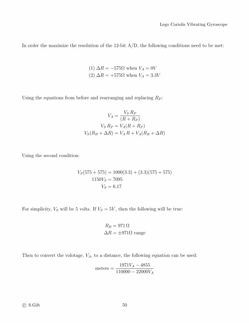
In order the maximize the resolution of the 12-bit A/D, the following conditions need to be met:

(1) ∆R = −575Ω when VA = 0V

(2) ∆R = +575Ω when VA = 3.3V

Using the equations from before and rearranging and replacing RP :

VA =VS RP

(R +RP )

VS RP = VA(R +RP )

VS(RB + ∆R) = VAR + VA(RB + ∆R)

Using the second condition:

VS(575 + 575) = 1000(3.3) + (3.3)(575 + 575)

1150VS = 7095

VS = 6.17

For simplicity, VS will be 5 volts. If VS = 5V , then the following will be true:

RB = 971 Ω

∆R = ±971Ω range

Then to convert the volotage, VA, to a distance, the following equation can be used:

meters =1971VA − 4855

110000− 22000VA

c© S.Gift 50


8

Software

Software was written to simulate the gyroscope and also to analysis the real and simulated data.The “Arduino ComPortScope” software is shown in figure 8.1. This software reads in the data fromthe Arduino microcontroller into a data file on the computer. The “Lego Gyro Sim” software isshown in figure 8.2. This software not only simulated the gyroscope, it also processed the raw datainto sensed rate. Figure 8.3 is an example of processed simulated data from a simulated multi-ratetest.

Figure 8.1: Arduino ComPortScope Software Screenshot

c© S.Gift 51


Figure 8.2: Lego Gyro Sim Software Screenshot

Figure 8.3: Example of Processed Simulated Multi-Rate Test

c© S.Gift 52


9

Testing Effort

Table 9.1 contains the list of tests conducted for this project. Figure 9.1 is a photograph of theLego gyro on a cordless drill at the house. The cordless drill was used as a rate table to verify thegyro actually did measure rate. Figure 9.2 shows the data for this test. Figure 9.3 is a photographof the data on the precision rate table at NRDC. Figure 9.4 is the data from test 1003.

Number Description

1001 Test conducted at house with a drill1002 Multi-rate test at NRDC, problem with the rate table1003 Multi-rate test at NRDC1004 Stability test at NRDC1005 Impulse response test at house

Table 9.1: Tests Conducted

c© S.Gift 53


Figure 9.1: At the House on the Drill

Figure 9.2: Test 1001 Time Data

c© S.Gift 54


Figure 9.3: On the Rate Table

Figure 9.4: Test 1003 Time Data

c© S.Gift 55



c© S.Gift 56


10

Results

10.1 Homogeneous Solution Results

The homogeneous solution to the differential equation along the sense axis is useful in determiningthe system’s parameters. The mass (m) of the system for the Lego gyroscope was determined bymeasurement with a scale. The spring (k) and damper (c) terms were determined by physicallymoving the Lego gyroscope’s mass to the left or right along the sense axis then letting go; thesystem would then oscillate with an exponential decay. This type of response is expected andshown by the solution to the homogeneous equation. It is also noted that the Lego gyroscope wascreated purposely this way. The homogeneous equation is then set to the initial conditions and theconstants (C1 and C2) are solved for.

yh = C1e−tτ cos(ωt) + C2e

−tτ sin(ωt)

yh =−tτC1e

−tτ cos(ωt)− C1ωe

−tτ sin(ωt)− t

τC2e

−tτ sin(ωt) + C2

−tτe

−tτ cos(ωt)

τ =2m

c

ω =

√4mk − c2

2m

c© S.Gift 57


The initial conditions are defined as:

y(0) = A [meters]

y(0) = B [meters/sec]

where A and B are given. For the test y(0) = 0.035 and y(0) = 0. The solutions to C1 and C2 are:

C1 = A (10.1)

C2 =B + A

τ

ω(10.2)

Actual measured response of the system when “let go” was collected. This data was then fit to theanalytical solution derived in equations 10.1 to 10.2 to determine the spring and damper terms ofthe Lego gyroscope. Two tests were executed. Test-A started the mass over at -44.1 mm. Test-Bstarted the mass over at +35.0 mm. These parameters are summarized in table 10.1.

Parameter Units Test-A Test-B

Start Time sec 24.60 28.00Initial Y mm -44.10 +35.00“Let Go” Time sec 24.96 28.12End Time sec 25.80 28.90

Table 10.1: Homogeneous Solution Fit Parameters

c© S.Gift 58


A range of spring (k) and damper (c) terms were used to create a fit to the measured data. At eachstep, the standard deviation of residuals were calculated from the measured data to the fit data.This created a two-dimensional plot of k, c, and standard deviation of residuals. Figures 10.1 and10.2 show these two-dimensional plots. The results from the plots are summarized in table 10.2.Test-A and Test-B showed matching results.

Parameter Units Test-A Test-B Average

c kg/sec 4.9 5.3 5.1k N/meter 192 212 202

Table 10.2: Homogeneous Solution Fit Solution

Figure 10.3, and 10.4 show the measured data for each test and and best fit as determined fromfigures 10.1 and 10.2.

c© S.Gift 59


Figure 10.1: Two dimensional plot of residuals from the homogeneous solution fit for Test-A

Figure 10.2: Two dimensional plot of residuals from the homogeneous solution fit for Test-B

c© S.Gift 60


Figure 10.3: Measured data from the Lego gyroscope (blue) and best homogeneous solution fit (red)for Test-A

Figure 10.4: Measured data from the Lego gyroscope (blue) and best homogeneous solution fit (red)for Test-B

c© S.Gift 61


10.2 Bias-instability and ARW Results

A test was conducted to measure the bias-instability and the Angle Random Walk (ARW). Thesensor was stationary and data was saved at 100 Hz for 1.4 hours. Figure 10.5 shows the data overtime. Figure 10.6 shows the Allan-deviation of this data in deg/sec. The minimum of this plot isthe bias-instability after it divided by 0.6 and then multiplies by 3600 to get it into deg/hr. Figure10.7 shows Power Spectral Density (PSD) plot of the data. From this plot the gyroscope ARWcan be calculated. The mean of the selected area is then multiplies by 60 to get it into deg/

√hr.

Table 10.3 list these results.

Parameter Units Result

Bias deg/hr 14509Standard Deviation deg/hr 1-σ 42414Bias-instability deg/hr 11370

ARW deg/√

hr 1063

Table 10.3: Bias-instability and ARW Results

c© S.Gift 62


Figure 10.5: Data verses Time

Figure 10.6: Allan-Deviation

Figure 10.7: PSD Plot

c© S.Gift 63


10.3 Scale Factor Results

A test was conducted with precision rate table. The table was rotated at ±100 deg/sec, ±150deg/sec, and ±190 deg/sec. Data was recorded throughout the test effort. From the data collected,a linear fit was applied to the gyro output versus the input rate. This fit is show in Figure 10.8.The Lego gyroscope scale factor was determined to be 33333 deg/sec/output. The Lego gyroscopein-run bias was determined to be -143 deg/sec. The fit also shows a large scale factor non-linearitywhich was expected because of the Lego design using rubber bands for the springs.

Figure 10.8: Lego Gyroscope Output vs Input Rate

c© S.Gift 64


Bibliography

[1] Paper on Equations of Motion For Rotating Frames, Nick Saluzzi, 2012

[2] Calculus, 3rd Edition, James Stewart, Brooks / Cole Publishing Company, 1995 (ISBN 0 534-21798-2)

[3] Elementary Differential Equations, 3rd Edition,C.H. Edwards, Jr, David E. Penny, Prentice-HallInc, 1993 (ISBN 0-13-253410-X)

[4] Dynamic Modeling and Control of Engineering Systems, Second Edition, J. Lowen Shearer,Bohdan T. Kulakowski, John F. Gardner, Prentice Hall, 1997 (ISBN 0-13-356403-7)

[5] IEEE Standard Specification Format Guide and Test Procedure for Single-Axis InterferometricFiber Optic Gyros, IEEE Standard 952-1997 (R2008).

[6] IEEE Standard Specification Format Guide and Test Procedure for Linear, Single-Axis, Non-Gyroscopic Accelerometers, IEEE Standard 1293-1998 (R2008).

c© S.Gift 65

Documents

Lego Coriolis Vibrating GyroscopeLego Coriolis Vibrating Gyroscope 1 Introduction This document describes the design of a Coriolis vibrating gyroscope created out of Legos. The purpose