Embed Size (px)
Citation preview

Front. Electr. Electron. Eng. China 2011, 6(1): 86–119
DOI 10.1007/s11460-011-0135-1
Lei XU
Codimensional matrix pairing perspective of BYY harmony
learning: hierarchy of bilinear systems, joint decomposition
of data-covariance, and applications of network biology
c© Higher Education Press and Springer-Verlag Berlin Heidelberg 2011
Abstract One paper in a preceding issue of this jour-nal has introduced the Bayesian Ying-Yang (BYY) har-mony learning from a perspective of problem solving,parameter learning, and model selection. In a comple-mentary role, the paper provides further insights fromanother perspective that a co-dimensional matrix pair(shortly co-dim matrix pair) forms a building unit and ahierarchy of such building units sets up the BYY system.The BYY harmony learning is re-examined via explor-ing the nature of a co-dim matrix pair, which leads toimproved learning performance with refined model selec-tion criteria and a modified mechanism that coordinatesautomatic model selection and sparse learning. Besidesupdating typical algorithms of factor analysis (FA), bi-nary FA (BFA), binary matrix factorization (BMF), andnonnegative matrix factorization (NMF) to share such amechanism, we are also led to (a) a new parametriza-tion that embeds a de-noise nature to Gaussian mixtureand local FA (LFA); (b) an alternative formulation ofgraph Laplacian based linear manifold learning; (c) a co-decomposition of data and covariance for learning regu-larization and data integration; and (d) a co-dim matrixpair based generalization of temporal FA and state spacemodel. Moreover, with help of a co-dim matrix pair inHadamard product, we are led to a semi-supervised for-mation for regression analysis and a semi-blind learningformation for temporal FA and state space model. Fur-thermore, we address that these advances provide withnew tools for network biology studies, including learn-ing transcriptional regulatory, Protein-Protein Interac-tion network alignment, and network integration.
Received December 1, 2010; accepted January 7, 2011
Lei XU
Department of Computer Science and Engineering, The ChineseUniversity of Hong Kong, Hong Kong, China
E-mail: [email protected]
Keywords Bayesian Ying-Yang (BYY) harmonylearning, automatic model selection, bi-linear stochasticsystem, co-dimensional matrix pair, sparse learning, de-noise embedded Gaussian mixture, de-noise embeddedlocal factor analysis (LFA), bi-clustering, manifold learn-ing, temporal factor analysis (TFA), semi-blind learn-ing, attributed graph matching, generalized linear model(GLM), gene transcriptional regulatory, network align-ment, network integration
1 Introduction
Firstly proposed in 1995 and systematically developedover a decade, the Bayesian Ying Yang (BYY) harmonylearning provides not only a general framework that ac-commodates typical learning approaches from a unifiedperspective but also a new road that leads to improvedmodel selection criteria, Ying-Yang alternative learningwith automatic model selection, as well as coordinatedimplementation of Ying based model selection and Yangbased learning regularization. In one preceding issueof this journal [1], one paper provided the fundamen-tals of the BYY harmony learning, the basic implement-ing techniques, and a tutorial on algorithms for typicallearning tasks.
As shown by Fig. 2(d) in Ref. [1], an intelligent systemis believed to jointly perform a mapping X → R thatprojects a set X of observations into its correspondinginner representation R and also a mapping R → X thatreconstructs or interprets X from the inner representa-tion R, which are described via the joint distribution ofX , R in two types of Bayesian decompositions:
Ying : q(X,R) = q(X |R)q(R),
Yang : p(X,R) = p(R|X)p(X). (1)
In a complement of the Ying-Yang philosophy, we call
Lei XU. Co-dimensional matrix-pairing perspective of BYY harmonylearning 87
this pair BYY system. The Ying is primary, and theprobabilistic structures of q(X |R) and q(R) come fromthe natures of learning tasks. The Yang is secondary,and p(X) comes from a set of observation samples, whilethe probabilistic structure of p(R|X) is a functional withq(X |R), q(R) as its arguments, designed from Ying ac-cording to a Ying-Yang variety preservation principle.A Ying- Yang best harmony principle is proposed forlearning all the unknowns in the system, mathematicallyimplemented by maximizing the harmony functional:
H(p‖ q) =∫p(R|X)p(X) ln [q(X |R)q(R)]dRdX. (2)
From the standard perspective of Ref. [1], the inner rep-resentation R of a set of observation samples X = {xt}consists of three types that correspond to three inverseproblems, as shown by Fig. 2 in Ref. [1]. One is Y = {yt}of the inner coding vector yt per sample xt. Usually, themapping X → Y performs problem solving, called thefirst level inverse problem. The second type of inner rep-resentation consists of a parameter set Θ, and the map-ping X → Θ is the second level inverse problem calledparameter learning. The third type is k that consists ofone or several integers that closely relate to the complex-ities of Y and Θ, and X → k is the third level inverseproblem called model selection. Further details are re-ferred to Sect. 1.1 in Ref. [1]. Instead of this standardperspective, this paper provides further insights on theBYY harmony learning from a new perspective that aco-dimensional matrix pair (shortly co-dim matrix pair)
forms a building unit and a hierarchy of such buildingunits sets up the BYY system.
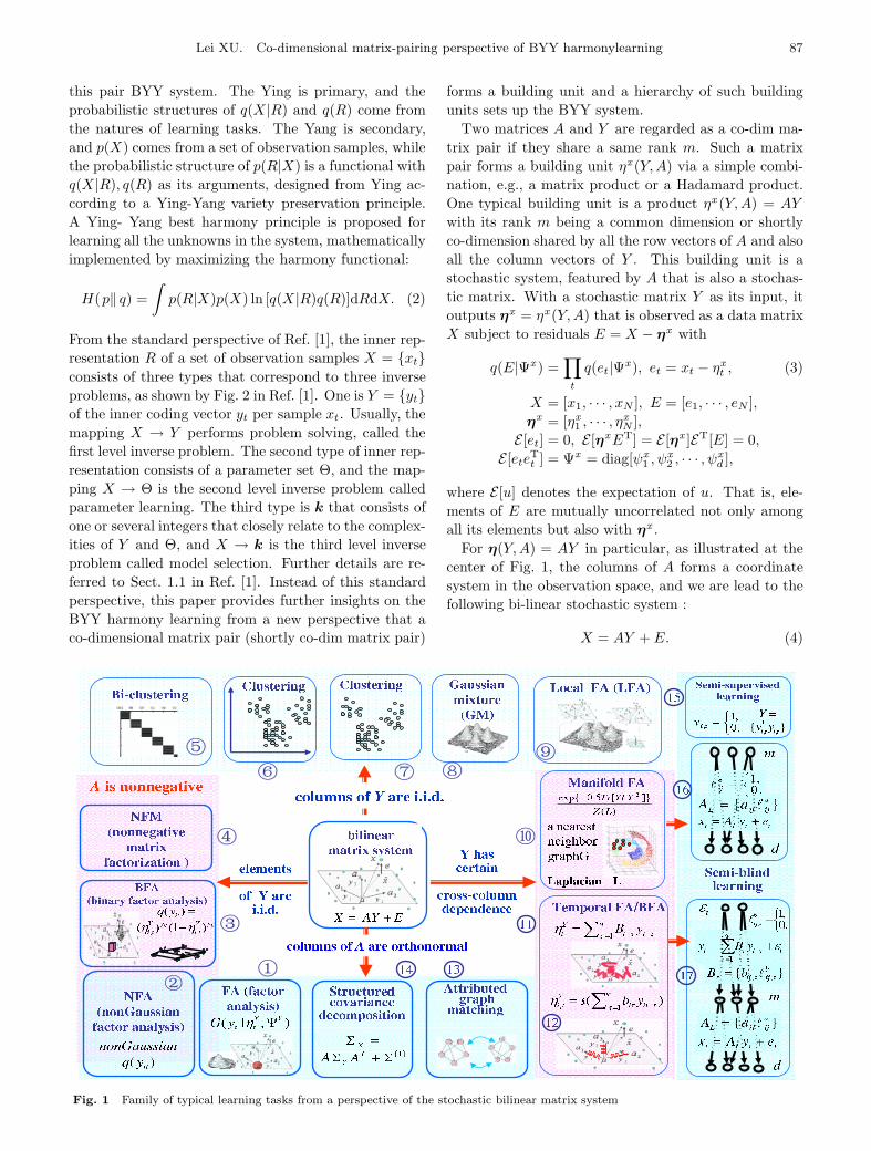
Two matrices A and Y are regarded as a co-dim ma-trix pair if they share a same rank m. Such a matrixpair forms a building unit ηx (Y,A) via a simple combi-nation, e.g., a matrix product or a Hadamard product.One typical building unit is a product ηx (Y,A) = AY
with its rank m being a common dimension or shortlyco-dimension shared by all the row vectors of A and alsoall the column vectors of Y . This building unit is astochastic system, featured by A that is also a stochas-tic matrix. With a stochastic matrix Y as its input, itoutputs ηx = ηx (Y,A) that is observed as a data matrixX subject to residuals E = X − ηx with
q(E|Ψx ) =∏t
q(et|Ψx ), et = xt − ηxt , (3)
X = [x1, · · · , xN ], E = [e1, · · · , eN ],ηx = [ηx1 , · · · , ηxN ],
E [et] = 0, E [ηxET] = E [ηx ]ET[E] = 0,E [eteTt ] = Ψx = diag[ψx
1 , ψx2 , · · · , ψx
d ],
where E [u] denotes the expectation of u. That is, ele-ments of E are mutually uncorrelated not only amongall its elements but also with ηx .
For η(Y,A) = AY in particular, as illustrated at thecenter of Fig. 1, the columns of A forms a coordinatesystem in the observation space, and we are lead to thefollowing bi-linear stochastic system :
X = AY + E. (4)
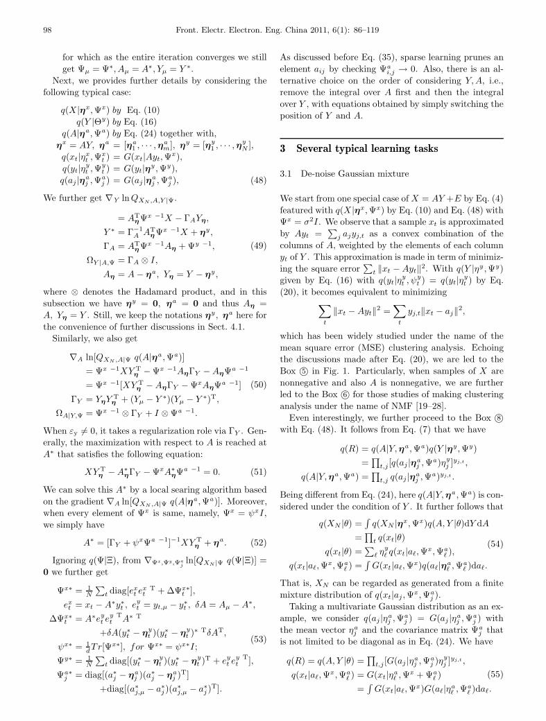
Fig. 1 Family of typical learning tasks from a perspective of the stochastic bilinear matrix system
88 Front. Electr. Electron. Eng. China 2011, 6(1): 86–119
To be further addressed in Sect. 2.1, typical learn-ing tasks are revisited when different constraints are im-posed on Y , A, and X . It follows from the Boxes 1©– 3©in Fig. 1 that we are led to a family of FA [2–4] and inde-pendent FA extensions [5–18], and from the Boxes 4©– 6©that we are led to a family of nonnegative matrix fac-torization (NMF) [19–28]. Also, we are led to not onlya new parametrization that embeds a de-noise nature toGaussian mixture [29–36] as shown in the Boxes 7©– 8©,but also an alternative formulation of graph Laplacianbased manifold learning [37,38] as shown in the Box 10©.
Extensive efforts have been made on learning X =AY + E under the principle of the least square errors(i.e., minimizing Tr[EET]), or generally the principle ofmaximizing the likelihood ln q(X |Θ) to estimate Θ of un-known parameters with a probabilistic structure q(X |Θ).One major limitation is that the rank of Y needs to beknown in advance. The problem is tackled with the helpof the Bayesian approach in two typical ways. One isdirectly maximizing
ln[q(X |Θ)q(Θ|Ξ)], (5)
with help of a priori q(Θ|Ξ), e.g., as encountered inlearning Gaussian mixture by minimum message length(MML) [39,40], and in sparse learning that prunes awayextra weights by a Laplace prior q(Θ|Ξ) for a regres-sion or interpolation task [41–43]. However, a choice ofq(Θ|Ξ) directly affects the estimation of Θ, and thus theperformance is sensitive to whether an appropriate pri-ori q(Θ|Ξ) is available. The other way is maximizing anapproximation of the marginal likelihood
q(X) =∫q(X |Θ)q(Θ|Ξ)dΘ, (6)
e.g., Bayesian inference criterion (BIC) [44], minimumdescription length (MDL) [45,46], and variational Bayes[47–49]. Details are referred to Sect. 2.1 of Ref. [1].
As shown in Fig. 5 of Ref. [1], the BYY harmonylearning on Eq. (4) leads to improved model selection viaeither or both of improved selection criteria and Ying-Yang alternative learning with automatic model selec-tion, with help of not only the role of q(Θ|Ξ) as abovebut also the role of q(Y |Θy). In this paper, as to bestated in Sect. 2.2, the BYY harmony learning is madeon a BYY system by Eq. (1) with
q(R) = q(Y − ηy |Ψy)q(A− ηa |Ψa)q(Υ), (7)
which differs from the following one in Ref. [1]:
q(R) = q(Y |Θy)q(Θ). (8)
That is, A is taken out of Θ = A ∪ Υ and is consideredin a paring with q(Y − ηy |Ψy) in order to explore thenature of co-dimension matrix pair A, Y . We are fur-ther led to improved learning performances with refined
model selection criteria and an interesting mechanismthat coordinates automatic model selection and sparselearning.
Complementarily, the data decomposition by Eq. (4)is associated with a decomposition of the data covari-ance SX into the covariance SY of Y and the covarianceΣ of E in a quadratic matrix equation
SX = ASYAT + Σ. (9)
There are also typical tasks that aim at this decomposi-tion with X unavailable but SX and SY available. Illus-trated in the Boxes 13©– 14© at the bottom of Fig. 1, onetype of such tasks is encountered by graph isomorphismand attributed graph matching [50–54], where SX andSY describe two unidirectional attributed graphs, whileA is a permutation matrix and Σ stands for matchingerrors. The other type of tasks comes from the sig-nal processing literature [55,56], where SX is a positivesemi-definite Toeplitz matrix, SY is diagonal, and A isparticularly structured with every element in a form ofexp[j(k − 1)ωl].
Given E that satisfies Eq. (3), making data decompo-sition by Eq. (4) implies the decomposition by Eq. (9),while making Eq. (9) also leads to Eq. (4) if we alsohave one additional condition that A is orthogonal andΣ = σ2I, as encountered in principal component analysis(PCA) [2,13]. In practice, the additional condition maynot hold, which is alternatively enhanced via makingboth the decompositions by Eq. (4) and Eq. (9). More-over, this co-decomposition provides a formulation thatintegrates different data types, namely X and SX . Also,making the decomposition by Eq. (9) can be regardedas imposing a structural regularization on learning themodel by Eq. (4).
According to the natures of learning tasks, the build-ing unit by Eq. (4) may further get supported from anupper layer. In addition to the standard way of usinga prior q(Θ|Ξ) in Eq. (8), either or both of ηy ,ηa mayalso itself be the output of another co-dim matrix paire.g., in a format of Eq. (4), which may be regarded asstructural priors. Moreover, either or both of Ψy and Ψa
may itself be the output of another co-dim matrix pairin a format of Eq. (9). So on and so forth, one new layermay have its next new layer. Whether we add a newupper layer depends on if there is some priors availableor we want to simplify computation. As a whole, a BYYsystem is featured by a hierarchy of co-dim matrix pairs.
To be specific, we consider two typical examples fea-tured with a two layer hierarchy. With ηa = ηa(ζ,Φ),the de-noise nature of the above new parametrization isalso embedded to a Gaussian mixture within a dimen-sion reduced subspace and further to local FA [57–67] asillustrated in the Box 9©. With ηy = ηy(ε, B), we arefurther led to a co-dim matrix pair based generalization
Lei XU. Co-dimensional matrix-pairing perspective of BYY harmonylearning 89
of temporal FA and structural state space model [68–75],as illustrated in the Boxes 11© and 12©.
Featured with merely data X available, all the abovediscussed tasks belong to what called unsupervisedlearning on Eq. (4). With both X and its correspondingY available, the problem becomes linear regression anal-ysis or a special example of supervised learning on Eq.(4). There are also many practical cases that are some-where a middle of the two ends. One example is thatthe corresponding columns of both X and Y are par-tially known in addition to merely having X available.Another example is encountered on studying what callednetworks component analysis (NCA) for transcriptionalregulation networks (TRN) in molecular biology, whereA is known to be sparse and the locations of zero ele-ments are known [76–79]. In fact, the two examples areinstances of a general scenario that we know not onlythe output observations X of a system but also partiallyeither or both of the input Y and the system (i.e., A andthe property of E).
Instances of this scenario were also encountered in thesignal processing studies on the linear convolution sys-tem, a special type of X = AY + E. The term blinddeconvolution [80,81] refers to the tasks of estimatingunknowns only from its output observations X , whilesemi-blind deconvolution [82] refers to the cases thatwe know partially either or both the system and its in-put. Moreover, instances of this scenario are also foundin those efforts made under the term semi-supervisedlearning [83] for pattern classification. The columns ofX are observed patterns from the outputs of a systemthat generates samples of selected classes, based on theinput Y with its columns indicating which classes toselect. We observe that semi-blind deconvolution andsemi-supervised learning share a similar concept but dif-fer in a specific system and specific types of input andoutput. Probably, semi-blind learning is a better namefor efforts that put attention on the general scenario ofknowing partially either or both of system and input.
In Ref. [1, Sect. 4.4], the BYY system is shown to pro-vide a unified framework to accommodate various casesof semi-supervised learning. To be stated in Sects. 3.2and 4.3, we are further led to a general formulation forsemi-blind learning. As illustrated in Fig. 1 from theBox 15© to the Box 17©, letting Y in Eq. (4) to be sup-ported from its upper layer by a Hadamard product ofco-dim matrix pair, we are lead to a formation of semi-supervised learning for regression analysis with a natureof automatic selection on variables; while letting A tobe supported from its upper layer by another Hadamardproduct of co-dim matrix pair, we are lead to a formationof semi-blind learning for Eq. (4) that covers the abovementioned NCA [76–79] as a special case. This forma-tion is further generalized for temporal modeling, withY supported by ηy(ε, B) and then B further supported
by a Hadamard product of another co-dim matrix pair.Last but not least, this paper also explores molecular
biology applications of the advances achieved from thenew perspective of the BYY harmony learning.
The existing studies on molecular networks rely ontechnologies available for data gathering, featured bytwo waves. The first is driven by a large number of”genome” projects on transcriptome mechanisms andparticularly TRN in the past two decades. In Sect.5.2, the past TRN studies will be summarized in threestreams of advances, and further progresses are sug-gested in help with the co-dim matrix pair perspective ofthe BYY harmony learning on X = AY + E, especiallythe general formulation for semi-blind learning and itsextension for temporal modeling.
The second wave is featured by the term interac-tome, due to recent large-scale technologies for measur-ing protein-to-protein interactions (PPIs) [84]. PPI dataare represented by undirectional networks or graphs, andtwo major tasks on PPI data are graph partitioningfor module detection and graph matching for networkalignment. Recently, a BYY harmony learning based bi-clustering algorithm has also been developed for graphpartitioning and shown favorable performances in com-parison with several well known clustering algorithms forthe same purpose [28]. Further improvements are sug-gested from the co-dim matrix pair perspective in thispaper. Moreover, the problem of network alignment isalso taken in consideration with graph matching algo-rithms from the perspective of Eq. (9) with help of theBYY harmony learning.
Additionally, there are several data sources availablefor the studies of transcriptome mechanisms, which leadto different networks and thus arise the needs of net-work integration. A similar scenario is also encounteredfor the studies of interactome mechanisms. Actually,two domains of mechanisms are related too. Therefore,network integration becomes increasingly important inthe current network biology studies [85]. The problemof network integration is closely coupled with networkalignment, and the co-decomposition by Eq. (4) and Eq.(9) provides a potential formulation for integrating datatypes across the domains.
The rest of this paper is arranged as follows. Sec-tion 2 starts from a bi-linear stochastic system and itspost-linear extensions, together with a brief outline oftypical learning tasks it covers. Then, a joint considera-tion of a co-dim matrix pair is shown to further improvethe BYY harmony learning, with a new mechanism thatcoordinates automatic model selection and sparse learn-ing. In Sect. 3, we get further insights on this perspec-tive of the BYY harmony learning via examples basedon Eq. (4). In addition to updating typical algorithmsof the FA and NFA families to share such a mechanism,we suggest a new parametrization that embeds a de-
90 Front. Electr. Electron. Eng. China 2011, 6(1): 86–119
noise nature to Gaussian mixture and variants, and analternative formulation of graph Laplacian based linearmanifold learning. Then, taking Eq. (9) also in consid-eration, we are led to algorithms for attributed graphmatching and a co-decomposition of data and covari-ance. In Sect.4, we proceed to a general formulationof a BYY harmony learning with a hierarchy of sev-eral co-dim matrix pairs. The de-noise parametrizationhas been further extended to local FA, and the co-dimmatrix pairing nature has been generalized to temporalFA and state space modeling. Moreover, with help of aco-dim matrix pair in Hadamard product, we are leadto a general formation of semi-blind learning. Finally,section 5 further addresses that these advances providewith new tools for network biology applications, includ-ing learning TRN, PPI network alignment, and networkintegration.
2 Co-dimensional matrix-pairing perspectiveof BYY harmony learning
2.1 Learning post bi-linear system and model selection
This subsection introduces the probabilistic structuresfor q(X |ηx ,Ψx ), q(Y |Θy) and q(A|ηa ,Ψa), and relatedfundamental issues, including typical learning tasks, in-determinacy problems, and model selection issues.
Equivalently, q(E|Ψx ) in Eq. (3) can be rewritten into
X = ηx + E,
q(X |R) = q(X |ηx ,Ψx ) = q(X − ηx |Ψx ),=
∏t q(xt − ηxt |Ψx
t ) =∏t q(xt|ηxt ,Ψx
t ),
ηxt = E [xt],
Ψxt = E [(xt − ηxt )(xt − ηxt )T] = E [eteTt ] by Eq.(4),
(10)
where the nations q(u|ηu ,Ψu) and q(u − ηu |Ψu) areused exchangeably for convenience. Typically, for xt =[x1,t, · · · , xd,t]T we also have
q(xt|ηxt , ψxt ) =
∏j q(xj,t|ηxj,t, ψx
j,t). (11)
From knowing that elements of the additive noise Ehave zero mean and are uncorrelated among all its ele-ments and also with ηx , we further have
E [vec(X)vecT(X)] = E [vec(ηx )vecT(ηx )]
+E [vec(E)vecT(E)].(12)
This is a problem of additive decomposition of a non-negative definite matrix into a sum of two nonnegativedefinite matrices. Without knowing the noise covarianceE [vec(E)vecT(E)], we have an additive indeterminacythat the decomposition is ill-posed since there are infinitenumber of possibilities. To reduce the indeterminacy, we
may further impose some structure on a diagonal matrixE [vec(E)vecT(E)]. E.g., we have
E [vec(E)vecT(E)] = diag[Ψx , · · · ,Ψx ],
or Ψxt = Ψx ,
(13)
i.e., each row of E has a same covariance. At one ex-treme case, we even assume that all the elements of Eshares a same covariance σ2 as follows
Ψx = σ2I, or ψxj,t = σ2. (14)
Even in this case, the additive indeterminacy is still nottotally eliminated as long as E [vec(ηx )vecT(ηx )] +γIand σ2 − γ both remain nonnegative for any scalar γ.
The other way to reduce this indeterminacy is takingthe structure of ηx in consideration. For ηx = AY inEq. (4), the above indeterminacy about a scalar γ maybe eliminated by the maximum likelihood learning whenthe rank of AY is less than the full rank d. However, theindeterminacy still remains when either AY is full rankor Ψx is diagonal. Moreover, it follows that
AY = Aφφ−1Y = A∗Y ∗,
A∗ = Aφ, Y ∗ = φ−1Y.(15)
i.e., AY suffers an indeterminacy of any nonsingular ma-trix φ.
To tackle the problem, we consider an appropriatestructural constraint on Y . A typical structure isthat its elements are independently distributed, that is,q(Y − ηy |Ψy) in Eq. (7) is given as follows:
q(Y |ηy ,Ψy) = q(Y − ηy |Ψy),
q(Y |ηy ,Ψy) =∏t q(yt|ηyt ,Ψy
t ),
q(yt|ηyt , ψyt ) =
∏j q(yj,t|ηyj,t, ψy
j,t),ηyt = E [yt],
Ψyt = E [(yt − ηxt )(xt − ηxt )T]
= diag[ψy1 , ψ
y2 , · · · , ψy
m],Y = [y1, · · · , yN ]T, yt = [y1,t, · · · , ym,t]T.
(16)
Similar to Eq. (13), in many problems [2–18], thecolumns of Y are independently and identically dis-tributed (i.i.d.), from which we have
Ψyt = Ψy . (17)
Moreover, the counterpart of Eq. (14) is also encounteredin some studies.
For ηx = AY in Eq. (4), ηx is regarded as gener-ated from independent hidden factors, which makes theindeterminacy of any nonsingular matrix φ in Eq. (15)reduces to an indeterminacy that φ comes from the or-thogonal matrix family. In this case, Eq. (10) coversseveral typical latent variable models shown in Fig. 1,with the following details :
Lei XU. Co-dimensional matrix-pairing perspective of BYY harmonylearning 91
• As illustrated by the Box 1©, we are lead to theclassic FA [2–4] for real valued Y featured with thateach yi,t is the following Gaussian
q(yj,t|ηyj,t, ψyj ) = G(yj,t|0, 1),
ηyj,t = 0, ψyj = 1,
q(yt|ηyt , ψyt ) = G(yt|0, I),
(18)
where and hereafter G(u|μ,Σ) denotes a Gaussiandistribution with a mean μ and a covariance matrixΣ. The indeterminacy of any orthogonal matrix φreduces to an orthonormal matrix since ψy
j = 1.• As illustrated by the Box 3©, we are lead to the bi-
nary FA (BFA) [5–8] with each yi,t = 0 or yi,t = 1from
q(yj,t |ηyj,t, ψyj ) = q(yj,t|ηyj,t)
= exp{yj,t ln ηyj +(1 − yj,t) ln (1 − ηyj )},ηyj,t = ηyj , ψy
j = ηyj (1 − ηyj ),
(19)
where ψyj is not a free parameter but a function of
ηyj,t that need not to be put in the distribution. Theindeterminacy by φ reduces to only any permuta-tion, since yi,t takes only 1 or 0.
• The above BFA includes a special case that has oneadditional constraint
yi,t = 0, yi,t = 1,∑i yi,t = 1,
q(yt|ηyt ) = exp{∑j yj,t ln ηyj },
∑j η
yj = 1.
(20)
That is, the hidden factors are not only binarybut also exclusively taking 1 by only one factor.Also, to be further introduced in Sect. 3.1 that thisexclusive BFA equivalently implements the classicleast square error (MSE) clustering problem, as il-lustrated by the Box 5©.
• As illustrated by the Box 2©, we are lead to the non-Gaussian FA (NFA) [9–13] for real valued Y that atmost one yi,t per column is Gaussian. In this case,we have a scale indeterminacy [86].
• As illustrated in the Boxes 4©– 6©, the NFA includesa family featured by that both A and Y are non-negative matrices, where a matrix is nonnegativeif every element is nonnegative valued. Extensivestudies has been widely made on this family underthe term nonnegative matrix factorization (NMF)[19–28]. Moreover, BFA and exclusive BFA alsolead to its NMF counterparts when A is a nonneg-ative matrix, as illustrated by the Box 7©.
Moreover, both BFA and NFA closely relate to multi-ple cause mixture model [14,15], and generalized latenttrait models or item response theory [16–18]. Particu-larly, Eq. (4) with Eq. (19) and Eq. (20) lead to twotypical binary matrix factorization (BMF) models [28]when the matrix A comes from a distribution similar toEq. (19) or a distribution similar to Eq. (20).
For a unified consideration on binary, real, and non-negative valued yi,t, we consider q(yi,t|ηyi,t, ψy
i ) in Eq.(16) given by the following exponential family [87]:
q(u|η, ψ) =
⎧⎨⎩
exp{ 1ψ
[ηu− a(η) − h(u)]}, (a) ,
G(u|η, ψ), (b).(21)
Generally, η, ψ are called natural parameter and disper-sion parameter, respectively. Corresponding to a specificdistribution, the function η(·) is also a specific scalarfunction called the mean function while its inverse func-tion η−1(r) is called the link function in the literatureof generalized linear model (GLM) [88]. Some examplesare shown in Table 1, e.g., we may consider Bernoulliand exponential distribution when ψ = 1 and u takesbinary and nonnegative values, respectively.
Table 1 Link functions for several typical distributions in theexponential family
distribution name link function mean function
Gaussian identity η−1(r) = r η(ξ) = ξ
exponential
gammainverse η−1(r) = r−1 η(ξ) = ξ−1
binomial
Bernoullilogit η−1(r) = ln
r
1 − rη(ξ) =
1
1 + exp(−ξ)
Similarly, we may consider q(xi,t|ηxi,t, ψxi ) coming from
the exponential family by Eq. (10) together with Table1, in order to cover that xi,t takes either of binary, real,and nonnegative types of values. Accordingly, we extendEq. (4) into the following one:
ηx =
{AY (a)homogenous linear,η(AY ), (b)post-linear
(22)
where η(V ) = [η(vi,j)] for a matrix V = [vi,j ]and a monotonic scalar function η(r),
by which X = ηx + E becomes a post bi-linear systemsince it is an extension of the bi-linear system by Eq. (4)with the bilinear unit AY followed by an element-wisenonlinear scalar mapping η(r). When both X and Y aregiven, the above model degenerates to the generalizedlinear model (GLM) for the linear regression [88].
A nonlinear scalar mapping η(r) in Eq. (22)(b) alsobring one additional favorable point. For Eq. (22)(a),the additive form by Eq. (12) gets the detailed form Eq.(9) for a fixed A. Observing ASYA
T + Σ = ASYAT +
C + Σ − C, there will be many values for C such thatboth ASYA
T+C and Σ−C remain nonnegative definite.Also, any nonnegative definite matrix can be rewrittenin the form A∗S∗
yA∗T. In other words, there is still an
additive indeterminacy. For Eq. (22)(b), ASYAT be-
comes E[η(AY )ηT(AY )], while E[η(AY )ηT(AY )] + C
usually may not be rewritten into the same format ofE[η(AY )ηT(AY )]. In other words, an additive indeter-minacy has been eliminated.
92 Front. Electr. Electron. Eng. China 2011, 6(1): 86–119
A post bi-linear system is described by Eq. (10)and Eq. (11) in help with Eq. (16) plus a specificq(yj,t|ηyj,t, ψy
j ), (e.g., either of Eq. (18), Eq. (19), andEq. (20)) to meet a specific learning task. The task ofestimating all the unknown parameters in the systemis called parameter learning, which is typically imple-mented under the principle of the maximum likelihood(ML), that is
Θ∗ = argmaxΘ ln q(X |Θ), Θ = {A,Ψx ,Θy},q(X |Θ) =
∫q(X |η(AY ),Ψx )q(Y |Θy)dY.
(23)
The maximization is usually implemented by the expec-tation maximization (EM) algorithm [3,5,10–12].
One major challenge for the ML learning is that therank of AY needs to be given in advance, while givingan inappropriate rank will deteriorate the learning per-formances. This challenge is usually tackled by modelselection, sparse learning, and controlling model com-plexity, which are three closely related concepts in theliterature of machine learning and statistics. The con-cept of model selection came from several decades ago onthe studies of linear regression for selecting the numberof variables [89,90], of clustering analysis for the numberof clusters [91], of times series modeling for the order ofautoregressive model [92]. The studies of this stream allinvolve to select the best among a family of candidatemodels via enumerating the number or order, and thususually referred by the term of model selection.
The concept of model complexity came from the ef-forts also started in the 1960’s by Solomonoff [93] onwhat later called Kolmogorov complexity [94]. Being dif-ferent from task dependent models, these efforts aimedat a general framework that is able to measure the com-plexity of any given model by the counts of a unit com-plexity by a universal gauge and then to build a mathe-matical relation between this model complexity and themodel performance (i.e., generalization error). One diffi-culty is how to get a universal gauge. A popular exampleis the so-called VC dimension [95] based theory on struc-tural risk minimization, while the other example is theso-called yardstick or universal model in the evolutionof MDL studies [45,46]. The other challenge is that theresulted mathematical relation between measured com-plexity and model performance is conceptually and qual-itatively important but difficult to be applied to a modelselection task in practice. Efforts have also been madetowards this purpose and usually lead to some rough es-timates, among which useful ones typically coincide withthe first stream.
Instead of measuring the complexity contributed fromevery unit complexity, sparse learning is a recent popu-lar topic that came from efforts on Laplace prior basedBayesian learning, featured by pruning away each ex-tra parameter for selecting variables in a regression or
interpolation task [41–43]. Though sparse learning andcontrolling model complexity are both working for a tasksimilar to model selection and often referred in certainconfusion, three concepts actually have different levelsof focuses.
For a post bi-linear system by Eq. (10) and Eq. (16),the concept of model selection is selecting the columndimension m of Y or the number of variables in yt. It isalso equivalent to selecting the row dimension of A, whilemodel complexity considers measuring the complexity ofthe entire system by counting a total sum contributedfrom every unit complexity by a universal gauge. Thismodel complexity is a function ofm and thus can be usedfor model selection. However, as above mentioned, thismodel complexity not only is difficult to be computedaccurately but also may contain an additional part thateven blurs or weakens the sensitivity on selecting m.Without measuring the contributions from every unitcomplexity and also being different from model selectionthat prunes away extra individual columns of A, sparselearning focuses on pruning away individual parametersin A per element.
Instead of tackling the difficulty of counting every unitcomplexity by a universal gauge or considering whethereach individual parameter should be pruned away, modelselection works on an appropriate middle level on whicha unit incremental is featured by a sub-model, e.g., onecolumn of the matrix Y . This feature not only avoidswasting computing cost on useless details but also useslimited information collectively for estimating reliablyan intrinsic scale that suits the learning tasks. For thesystem by Eq. (10) and Eq. (16), this intrinsic scale isthe dimension m.
Most of the existing studies on both model selectionand sparse learning rely on ceratin a priori q(Θ|Ξ). Fora post bi-linear system by Eq. (10) and Eq. (16), thefirst important a priori is about A. Recalling that thecolumns of A form a coordinate system in the observa-tion space, we let such a priori about A in a structure ofcolumn-wise independence as follows:
q(A− ηa |Ψa) = q(A|ηa ,Ψa) =∏j q(aj |ηa
j ,Ψaj ),
A = [a1, a2, · · · , am], ηa = [ηa1 ,η
a2 , · · · ,ηa
m],
Ψa = diag[ψa1 , ψ
a2 , · · · , ψa
m],
(24)
where q(aj |ηaj ,Ψ
a) comes from the following extensionof Eq. (21) for a multivariate vector u:
q(u|η, ψ) =
⎧⎪⎨⎪⎩eη
Tψ−1u−a(η,ψ)−h(u,ψ), (a),
G(u|η, ψ), (b),
ML(u|η, ψ), (c),
where ψ is usually a diagonal matrix for the case (a),and ML(u|η, ψ) denotes a multivariate Laplace extendedfrom its counterpart multivariate Gaussian G(u|η, ψ).
Lei XU. Co-dimensional matrix-pairing perspective of BYY harmonylearning 93
On one hand, extensive efforts have been made onlearning based a priori with help of Bayesian approaches.That is, the ML learning by Eq. (23) is extended intomaximizing Eq. (5) under the name of Bayesian learn-ing or maximizing Eq. (6) under the name of marginalBayes or its approximation under the name of variationalBayes. As outlined in Sect. 2 and especially Figs. 4&5of Ref. [1], these studies all base on a priori q(Θ|Ξ), in-cluding the one by Eq. (24) to make model selection andsparse learning, while the role of q(Y |Θy) by Eq. (16)is hidden behind the integral in Eq. (23) without takingits role.
On the other hand, via q(R) by Eq. (8) the BYY har-mony learning by Eq. (2) considers q(Y |Θy) in a rolethat is not only equally important to q(Θ|Ξ) but alsoeasy computing, while q(Θ|Ξ) is still handled in a waysimilar to Bayesian approaches. As addressed in Sect.2.2 of Ref. [1], the BYY harmony learning on Eq. (4)leads to improved model selection via either or both ofimproved model selection criteria and Ying-Yang alter-native learning with automatic model selection.
Conventionally, model selection is implemented in twostages. That is, enumerating a number of m and learn-ing unknown parameters at each m, and then select-ing a best m∗ by a model selection criterion, such asAIC/BIC/MDL. An alternative road of efforts is re-ferred as automatic model selection. An early effortmade since 1992 is rival penalized competitive learning(RPCL) [96,97,34] for clustering analysis and Gaussianmixture, with the cluster number k automatically de-termined during learning. Also, sparse learning can beregarded as implementing a type of automatic modelselection, e.g., it leads to model selection if the parame-ters of one entire column of A has been all pruned away.The above mentioned Bayesian approach may also beimplemented in a way of automatic model selection, e.g.,pruning extra clusters by a Dirichlet prior [40].
As outlined at the end of Sect. 2.1 in Ref. [1], auto-matic model selection is associated with a learning algo-rithm or principle with the following two features:
• there is an indicator ψ(θSR) on a subset θSR ofparameters that represents a particular structuralcomponent.
• during implementing this learning, there is an in-trinsic mechanism that drives
ψ(θSR) → 0, as θSR → a specific value, (25)
if the corresponding component is redundant.Thus, automatic model selection gets in effect via check-ing ψ(θSR) → 0 and then discarding its correspondingθSR. The simplest case is checking whether θSR → 0, atypical scenario encountered in Ref. [1].
In the rest of this section, q(A|ηa ,Ψa) is put intoEq. (7) and jointly considered with q(Y |Θy) such that
the BYY harmony learning on Eq. (4) further improvesmodel selection and sparse learning, with help of explor-ing the co-dimension nature of the matrix pair A, Y .
2.2 Co-dim matrix pair and BYY harmony learning
Two matrices A and Y are regarded as a co-dimensional(shortly co-dim) matrix pair if they share a same rankm.In the post bi-linear system by Eq. (10) and Eq. (22), aco-dim matrix pair A and Y forms a matrix product AYas a core building unit. Actually, the common rank m isan intrinsic dimension that is shared from two aspects:
m is shared by
{all the columns of Y, (a)all the rows of A. (b)
(26)
That is, there are two sources of information that couldbe integrated for a reliable estimation on this intrinsicco-dimension m.
In the studies of linear regression that estimates Awith both X and Y given, model selection is made onselecting the variables of each row in A with the help ofeither a criterion (e.g., Cp , AIC, BIC) [44,89,91] thattakes the number of variables in consideration with helpof a priori onA. In the studies of learning a post bi-linearsystem with X given and Y unknown, parameter esti-mation is made by the maximum likelihood on q(X |Θ)in Eq. (23), and model selection is made via Bayesianapproach by Eq. (5) or Eq. (6) with help of a priori onA. In these studies, model selection uses only the infor-mation from A, while the information from Y has notbeen used for model selection though it is used for es-timating A. In other words, the information of Y hasbeen ignored or even not been noticed in those previousstudies. In contrast, as addressed in Sect. 2.2 of Ref. [1],the BYY harmony learning considers the information ofY via q(Y |Θy) in a role that differs from that in Eq. (23)but is equally important to a priori on A, which leads toimproved model selection on m.
Taking the studies on the classic FA [2–4] for furtherinsights, it follow from Eq. (18) thatG(yj,t|0, 1) has beenwidely adopted in the literature of statistics for describ-ing each hidden factor, without unknowns to be esti-mated. Equivalently, there is no free parameter withinthis parametrization for describing Y . In Ref. [76, Item9.4], we considered a different FA parametrization by re-stricting the matrix A to be orthonormal matrix and re-laxing the extreme case G(yj,t|0, 1) to G(yj,t|0, ψy
j ) withone unknown ψy
j . The two FA parameterizations makeno difference on q(X |Θ) in Eq. (23) and thus are equiv-alent in term of the ML learning. In contrast, two FAparameterizations become different in term of the BYYharmony learning, as listed in Table 2 of Ref. [9]. Also, itwas experimentally found that the FA with G(yj,t|0, ψy
j )outperforms considerably the FA with G(yj,t|0, 1) [98],
94 Front. Electr. Electron. Eng. China 2011, 6(1): 86–119
which may be understood from observing that a un-known parameter ψy
j provides a room for a further im-provement by the BYY harmony learning.
Though the BYY harmony learning takes the informa-tion of Y in consideration of model selection via q(Y |Θy)by Eq. (16), the previous studies on the BYY harmonylearning uses the information from A in a way similarto Bayesian approach by Eq. (5) or Eq. (6), in lack of agood coordination with q(Y |Θy). For improvements, weneed further examine the effects of scale indeterminacy.
As discussed in the previous subsection, this productAY suffers from the indeterminacy by Eq. (15), which isremedied via requiring the row independence of q(Y |Θy)by Eq. (16). For a diagonal matrix φ = D �= γI, the in-determinacy by Eq. (15) is usually called the scalar in-determinacy, which can not be removed by Eq. (16) for areal valued Y . When each yi,t takes either 1 or 0, such ascale indeterminacy is not permitted, since Y ∗ = D−1Y
could not remain to be either 1 or 0. Alternatively, if yi,tis allowed to be binary of any two values, we still have ascale indeterminacy.
The studies of maximum likelihood and Bayesian ap-proach by Eq. (5) or Eq. (6) rely on q(X |Θ) in Eq. (23),which is insensitive to such a scale indeterminacy. Usu-ally ψy
j = 1 is imposed to remove this scale indetermi-nacy, e.g., in Eq. (18) for the classic FA [2–4]. WithG(yj,t|0, 1) relaxed to G(yj,t|0, ψy
j ), the BYY harmonylearning searches an appropriate value for each ψy
j , withan improved model selection. Still, there is a scale in-determinacy that is removed by imposing the constraintATA = I [8,9,13].
In sequel, we seek a coordinated consideration of bothq(Y |ηy ,Ψy) by Eq. (16) and q(A|ηa ,Ψa) by Eq. (24),
q(A|0,Ψa) = q(A|ηa ,Ψa)|ηa=0,
q(Y |0,Ψy) = q(Y |ηy ,Ψy)|ηy=0.
We again focus on the FA with G(yj,t|0, 1) and the FAwith G(yj,t|0, ψy
j ). Both the two FA parameterizationsare special cases of a family of FA variants featured witha transform
A∗ = AD−1, Y ∗ = DY, D is a diagonal, (27)
which is shortly called the FA-D family. As stated above,instances in the FA-D family are equivalent in term ofthe ML learning and Bayesian approach. In Ref. [1],the BYY harmony learning by Eq. (2) with q(R) by Eq.(8) is considered with q(A|0,Ψa) buried in q(Θ), whileq(Y |0,Ψy) =
∏tG(yt|0, D2) with different diagonal ma-
trices of D makes no difference on q(X |Θ) by Eq. (23)but indeed leads to a difference for the BYY harmonylearning.
With help of q(R) by Eq. (7) that jointly considersq(Y |0,Ψy) and q(A|0,Ψa), it follows from q(Y ∗|0,Ψy)= q(Y |0,Ψy)/|D| and q(A∗|0,Ψa) = |D|q(A|0,Ψa) that
the value of this q(R) and thus the harmony measureH(p||q) by Eq. (2) are invariant to Eq. (27). That is,all the variants in the FA-D family become equivalentto each other. Interestingly, the above two FA param-eterizations become equivalent again. This coordinatednature of a paired q(Y |0,Ψy) and q(A|0,Ψa) providesthe following new insights.
(1) This variant nature is different from the previ-ous one owned by the ML learning. Due to q(X |Θ) inEq. (23), any value for D has no difference and also nohelp for model selection. Thus, ψy
j = 1 is simply imposedto remove such a scale indeterminacy, while the aboveBYY harmony learning is able to use the informationof Y in consideration of model selection via q(Y |Θy).With q(R) by Eq. (8), two FA parameterizations makethe harmony measure H(p||q) by Eq. (2) different. How-ever, we still do not know which one is better though theFA with G(yj,t|0, ψy
j ) is experimentally shown to outper-form the FA with G(yj,t|0, 1) [98]. In contrast, with q(R)by Eq. (7), knowing that two FA parameterizations makeH(p||q) by Eq. (2) take the same value indicates that weneed to compare two FA parameterizations from aspectsother than from H(p||q).
First, the FA with G(yj,t|0, ψyj ) is better than the FA
with G(yj,t|0, 1) in term of being able to use the infor-mation of Y for model selection. Particularly, automaticmodel selection can be made via discarding the j-th di-mension as the BYY harmony learning drives
ψyj → 0, (28)
as a simple example of Eq. (25). Second, in comparisonwith a priori q(A|0,Ψa), q(Y |0,Ψy) is more reliable andeasy to use (see Sect. 2.2 of Ref. [1]), while an inappropri-ate q(A|0,Ψa) will deteriorate the overall performance.Third, it follows from Eq. (26) that Y has N columnsto contain the information about m while A has only drows, where we usually have N � d or even N � d.
(2) In those previous studies on the BYY harmonylearning [1], the role of a priori q(A|0,Ψa) is buriedin q(Θ|Ξ) that contributes to a model selection crite-rion roughly via the number of free parameters in Θas a whole. A paired consideration of q(Y |0,Ψy) andq(A|0,Ψa) in Eq. (7) also motivates to put the contribu-tion by q(A|0,Ψa) in a more detailed expression. E.g.,the model selection criterion by Eq. (18) in Ref. [1] ismodified into
2J(m) = ln |Ψx | + h2Tr[Ψx −1] +m ln(2πe)+
ln |Ψy | + dN [m ln(2πe) + ln |Ψa |] + nf (Θ),
(29)
where ln |Ψa | =∑
i,j ln Ψai,j, and the notations Ψx , Ψy
were changed from ones Σ and Λ in Sect. 3.2 of Ref. [1],adopting the notation system of this paper (see Fig. 2).Also, we may ignore nf (Θ) if there is no appropriate pri-ori. It is observed that the contribution from q(A|0,Ψa)is weighted by a ratio d/N , which echoes the discussion
Lei XU. Co-dimensional matrix-pairing perspective of BYY harmonylearning 95
made at the end of the above item (1). Similarly, wemay also modify the model selection criterions by Eqs.(13) and (19) in Ref. [1].
(3) In the previous studies on the FA withG(yj,t|0, ψy
j ) (e.g., see Sect. 3.2 in Ref. [1]), to normallymake automatic model selection with help of checkingEq. (28), the BYY harmony learning need to be imple-mented under the constraint of requiring ATA = I forremoving a scale indeterminacy. It follows that Eq. (27)leads to the following scalar indeterminacy:
ψy∗j = d2
jψyj , Ψa∗
j = d−2j Ψa
j . (30)
That is, it may occur that one element of Ψy∗ tendsto zero due to a unknown scaling d2
j → 0 that maysimultaneously make the counterparting Ψa∗
tend toinfinity. The constraint ATA = I can avoid this sce-nario. Moreover, a paired consideration of q(Y |0,Ψy)and q(A|0,Ψa) in Eq. (7) motivate to find a betterchoice.
It can be observed that the above scalar indeterminacycan also be avoided by the following constraint
Tr[Ψaj ] = const or simply Tr[Ψa
j ] = 1, (31)
which is a relaxation of ATA = I at a diagonal case
Ψaj = diag[ψa
1,j, · · · , ψad,j],
ψai,j = E [(aij − ηaij)
2].(32)
Noticing that ATA = I includes aTj aj = 1 and that
ψai,j is a variance of the random variable aij , we see
that∑
j a2ij = 1 actually leads to
∑j Ψa
i,j = 1 whenE [aij ] = 0. Inversely,
∑j Ψa
i,j = 1 does not necessarilylead to
∑j a
2ij = 1.
The alternatives of ATA = I also include
{∑i
|aij |γ}1/γ = 1, 0 < γ <∞, for every j, (33)
where the case γ = 2 includes∑
j a2ij = 1 as a special
case. Moreover, it can be observed that these cases areall within the FA-D family by Eq. (27) with
D = diag[d1, · · · , dm],
dj = 1/Tr[Ψaj ], for Eq. (30),
dj = 1/{∑i |aij |γ}1/γ for Eq. (33) .
(34)
(4) For the Bayesian approach by Eq. (5) or Eq. (6)with q(X |Θ) by Eq. (23), the constraint ψy
j = 1 alreadyshut down the contribution of q(Y |0,Ψy) to model selec-tion. Actually, model selection is implemented via dis-carding the j-th column ofA if the entire column aj → 0.Also, sparse learning is implemented via discarding oneelement aij if aij → 0. In contrast, the BYY harmonylearning improves model selection via either or both ofEq. (28) and Eq. (29), with help of one constraint by
either of Eq. (31), Eq. (33) and Eq. (34). Still, sparselearning can be performed since such a constraint willnot impede aij → 0.
Moreover, checking aij → 0 may also be improved bychecking whether
Ψai,j → 0. (35)
A coordinated implementation of Eq. (28) and Eq. (35)under the constraint of Eq. (31) (or one of its alterna-tives) form a good mechanism that coordinates auto-matic model selection and sparse learning.
(5) Adding extra constraint to remove a scale inde-terminacy has both a good side and a bad side. Thegood side is facilitating to make model selection andsparse learning by Eq. (28) and Eq. (35) and also re-ducing the targeted domain of solutions. The bad sideis that externally forcing the targeted domain not onlyincreasing computing cost but also make it easy to bestuck at some suboptimal solution. Thus, we considerhow to make model selection and sparse learning with-out imposing those constraints by Eq. (31), Eq. (33) andEq. (34). Instead of checking by Eq. (28) and Eq. (35),i.e., the simplest format θSR → 0 in Eq. (25), we con-sider ψ(θSR) → 0 with ψ(θSR) in a composite format. Itfollows from Eq. (30) that the scalar indeterminacy alsodisappears by considering the product ψy∗
j Ψa∗j . Thus,
we replace Eq. (28) with the help of
(a) Discard the j-th row of Y and also the j-th
column of A if ψ(θSR) = ψyj Tr[Ψa
j ] → 0, (36)
(b) Discard the aij of A if ψ(θSR) = ψyj ψ
ai,j → 0.
for the special case by Eq. (32).
When the j-th dimension of yt or equivalently the j-throw of Y is redundant, both Eqs. (36)(a) and (36)(b) willhappen for every i. In this case, they equivalently pruneaway the j-th dimension. If Eq. (36)(b) happens only forsome i, the corresponding elements in the j-th columnof A will be pruned away, that is, we are lead to sparselearning. In other words, both automatic model selec-tion and sparse learning are nicely coordinated. Also,it can be observed that Eq. (36)(a) returns back to Eq.(28) under the constraint by Eq. (31). In other words,Eq. (36)(a) is an integration of Eq. (28) and Eq. (31).
2.3 Apex approximation and alternation maximization
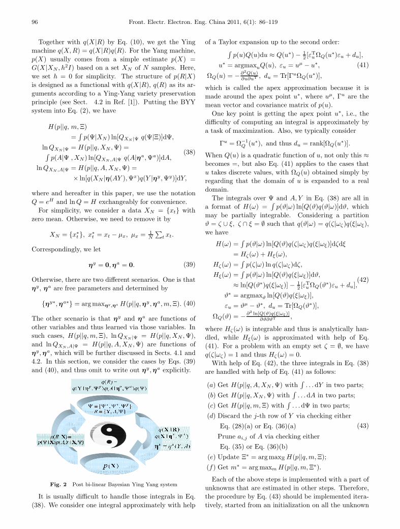
We further consider the Bayesian Ying Yang systemshown in Fig. 2, with the following representation
q(R) = q(Y |ηy ,Ψy)q(A|ηa ,Ψa)q(Ψ|Ξ),
Ψ = {Ψa ,Ψy ,Ψx}, (37)
which is a special case of Eq.(7) with Υ consisting ofonly Ψ while the rest parameters (if any) ignored.
96 Front. Electr. Electron. Eng. China 2011, 6(1): 86–119
Together with q(X |R) by Eq. (10), we get the Yingmachine q(X,R) = q(X |R)q(R). For the Yang machine,p(X) usually comes from a simple estimate p(X) =G(X |XN , h
2I) based on a set XN of N samples. Here,we set h = 0 for simplicity. The structure of p(R|X)is designed as a functional with q(X |R), q(R) as its ar-guments according to a Ying-Yang variety preservationprinciple (see Sect. 4.2 in Ref. [1]). Putting the BYYsystem into Eq. (2), we have
H(p||q, m,Ξ)
=∫p(Ψ|XN ) ln[QXN |Ψ q(Ψ|Ξ)]dΨ,
lnQXN |Ψ = H(p||q,XN ,Ψ) =∫p(A|Ψ , XN) ln[QXN ,A|Ψ q(A|ηa ,Ψa)]dA,
lnQXN ,A|Ψ = H(p||q, A,XN ,Ψ) =
× ln[q(XN |η(AY ),Ψx )q(Y |ηy ,Ψy)]dY,
(38)
where and hereafter in this paper, we use the notationQ = eH and lnQ = H exchangeably for convenience.
For simplicity, we consider a data XN = {xt} withzero mean. Otherwise, we need to remove it by
XN = {x∗t }, x∗t = xt − μx, μx = 1N
∑t xt.
Correspondingly, we let
ηy = 0,ηa = 0. (39)
Otherwise, there are two different scenarios. One is thatηy , ηa are free parameters and determined by
{ηy∗,ηa∗} = argmaxηy ,ηa H(p||q,ηy ,ηa ,m,Ξ). (40)
The other scenario is that ηy and ηa are functions ofother variables and thus learned via those variables. Insuch cases, H(p||q,m,Ξ), lnQXN |Ψ = H(p||q,XN ,Ψ),and lnQXN ,A|Ψ = H(p||q, A,XN ,Ψ) are functions ofηy ,ηa , which will be further discussed in Sects. 4.1 and4.2. In this section, we consider the cases by Eqs. (39)and (40), and thus omit to write out ηy ,ηa explicitly.
Fig. 2 Post bi-linear Bayesian Ying Yang system
It is usually difficult to handle those integrals in Eq.(38). We consider one integral approximately with help
of a Taylor expansion up to the second order:∫p(u)Q(u)du ≈ Q(u∗) − 1
2 [εTuΩQ(u∗)εu + du],
u∗ = argmaxuQ(u), εu = uμ − u∗,
ΩQ(u) = −∂2Q(u)∂u∂uT , du = Tr[ΓuΩQ(u∗)],
(41)
which is called the apex approximation because it ismade around the apex point u∗, where uμ, Γu are themean vector and covariance matrix of p(u).
One key point is getting the apex point u∗, i.e., thedifficulty of computing an integral is approximately bya task of maximization. Also, we typically consider
Γu = Ω−1Q (u∗), and thus du = rank[ΩQ(u∗)].
When Q(u) is a quadratic function of u, not only this ≈becomes =, but also Eq. (41) applies to the cases thatu takes discrete values, with ΩQ(u) obtained simply byregarding that the domain of u is expanded to a realdomain.
The integrals over Ψ and A, Y in Eq. (38) are all ina format of H(ω) =
∫p(ϑ|ω) ln[Q(ϑ)q(ϑ|ω)]dϑ, which
may be partially integrable. Considering a partitionϑ = ζ ∪ ξ, ζ ∩ ξ = ∅ such that q(ϑ|ω) = q(ζ|ωζ)q(ξ|ωξ),we have
H(ω) =∫p(ϑ|ω) ln[Q(ϑ)q(ζ|ωζ)q(ξ|ωξ)]dζdξ
= Hζ(ω) +Hξ(ω),
Hζ(ω) =∫p(ζ|ω) ln q(ζ|ωζ)dζ,
Hξ(ω) =∫p(ϑ|ω) ln[Q(ϑ)q(ξ|ωξ)]dϑ,
≈ ln[Q(ϑ∗)q(ξ|ωξ)] − 12 [εTuΩQ(ϑ∗)εu + du],
ϑ∗ = argmaxϑ ln[Q(ϑ)q(ξ|ωξ)],εu = ϑμ − ϑ∗, du = Tr[ΩQ(ϑ∗)],
ΩQ(ϑ) = −∂2 ln[Q(ϑ)q(ξ|ωξ)]∂ϑ∂ϑT ,
(42)
where Hζ(ω) is integrable and thus is analytically han-dled, while Hξ(ω) is approximated with help of Eq.(41). For a problem with an empty set ζ = ∅, we haveq(ζ|ωζ) = 1 and thus Hζ(ω) = 0.
With help of Eq. (42), the three integrals in Eq. (38)are handled with help of Eq. (41) as follows:
(a) Get H(p||q, A,XN ,Ψ) with∫. . . dY in two parts;
(b) Get H(p||q,XN ,Ψ) with∫. . .dA in two parts;
(c) Get H(p||q,m,Ξ) with∫. . .dΨ in two parts;
(d) Discard the j-th row of Y via checking either
Eq. (28)(a) or Eq. (36)(a)
Prune ai,j of A via checking eitherEq. (35) or Eq. (36)(b)
(e) Update Ξ∗ = argmaxΞH(p||q,m,Ξ);
(f) Get m∗ = arg maxmH(p||q,m,Ξ∗).
(43)
Each of the above steps is implemented with a part ofunknowns that are estimated in other steps. Therefore,the procedure by Eq. (43) should be implemented itera-tively, started from an initialization on all the unknown
Lei XU. Co-dimensional matrix-pairing perspective of BYY harmonylearning 97
parameters. The first four steps already composite oneiterative learning algorithm with automatic model selec-tion and sparse learning implemented at Step (d). Step(e) is involved only when there is a priori q(Ψ|Ξ)]. Also,Step (f) is made in a way similar to the conventional twostage implementation. That is, steps (a)-(e) are iterativeuntil convergence at each m, after enumerating m for anumber of value, a best m∗ is selected by the criterionfrom H(p||q,m,Ξ∗), e.g., the one in Eq. (29) for FA.
In Eqs. (43)(a)& (b) & (c), removing an integral in twoparts as handled in Eq. (43). For some problems, the en-tire integral is analytically integrable, and thus there isno part that needs to make approximation. Also, theremay be no analytically integrable part, for which the en-tire integral has to be tackled approximately. Usually,we need a trade-off between computing cost and accu-racy when the entire integral is divided into two parts.
Taking∫. . . dY for an example, when each yi,t takes
values by Eq. (20), the integral∫. . .dY becomes a sim-
ple summation, which definitely belongs to the part ofanalytically integrable. When each yi,t takes either 1 or0, the integral
∫. . . dY also becomes a summation, for
which we encounter a trading-off scenario. If the dimen-sion m is not high, this case may still be classified as thepart of analytically integrable. However, the computa-tional complexity of the summation becomes intractablefor a big value m. Such a situation should be classifiedinto the part to be handled approximately with help ofEq. (41).
In sequel, we introduce the detailed equations for theapproximations in Eqs. (43)(a)& (b) & (c). Without los-ing generality and also for notation simplicity, we onlyconsider how to handle the approximation part in Eq.(42), while the analytically integrable part is task de-pendent and handled manually.
We start from Step (a) to consider the integral∫. . . dY for getting H(p||q,ηy ,ηa ,m,Ξ) in Eq. (38). It
follows from Eq. (41) and Eq. (42) that we have
lnQXN ,A|Ψ = H(p||q, A,XN ,Ψ)=
∫p(Y |A,Ψ, XN) lnQXN ,A,Y |ΨdY.
= lnQXN ,A,Y ∗|Ψ− 1
2 [εTy ΩY ∗|A,Ψεy + dY ∗|A,Ψ]lnQXN ,A,Y ∗|Ψ = lnQXN ,A,Y=Y ∗|Ψ,
Y ∗ = argmaxA lnQXN ,A,Y |Ψ,
lnQXN ,A,Y |Ψ = ln[q(XN |η(AY ),Ψx )q(Y |ηy ,Ψy)],
εy = vec(Yμ − Y ∗),dY ∗|A,Ψ = rank[ΩY ∗|A,Ψ],
ΩY |A,Ψ = − ∂2 lnQXN ,A,Y |Ψ∂vec(Y )∂vec(Y )T .
(44)
We move to Step (b) to consider the integral∫. . . dA
for getting H(p||q,XN ,Ψ) in Eq. (38).
lnQXN |Ψ = H(p||q,XN ,Ψ)
= ln[QXN ,A∗|Ψq(A∗|ηa ,Ψa)]− 1
2 [εTa ΩA∗|Y ∗,Ψεa + dA∗|Y ∗,Ψ],
A∗ = argmaxA ln[QXN ,A|Ψ q(A|ηa ,Ψa)],
εa = vec(Aμ −A∗),dA∗|Y ∗,Ψ = rank[ΩA∗|Y ∗,Ψ],
ΩA|Y,Ψ = −∂2 ln[QXN ,A|Ψ q(A|ηa ,Ψa)]
∂vec(A)∂vec(A)T .
(45)
Next, we proceed to Step (c) to get the integral∫. . . dΨ
for getting H(p||q,m,Ξ) in Eq. (38) turned into
H (p||q,m,Ξ) =∫p(Ψ|XN ) ln[QXN |Ψ q(Ψ|Ξ)]dΨ
= ln[QXN |Ψ∗ q(Ψ∗|Ξ)] − 12 [εTΨ∗ΩΨ∗εΨ∗ + dΨ∗ ],
Ψ∗ = argmaxΨ ln[QXN |Ψ q(Ψ|Ξ)],
εΨ = vec(Ψμ − Ψ∗),
dΨ = rank[ΩΨ],
ΩΨ = −∂2 ln[QXN |Ψ q(Ψ|Ξ)]∂vec(Ψ)∂vec(Ψ)T
.
(46)
In the above equations, the following computing issuesneed to be further addressed:
• Only for some special cases, the implementations ofmaxY , maxA, and maxΨ are analytically solvable.Generally, a maximization with respect to contin-uous variables is implemented by a gradient basedsearching algorithm, suffering a local maximizationproblem, while a maximization with respect to dis-crete variables, e.g., each yi,t takes either 1 or 0,involves a combinatorial optimization [99,100].
• The Hessian matrices ΩY |A,Ψ, ΩA|Y,Ψ, and ΩΨ aretypically assumed to be diagonal for avoiding te-dious computation and unreliable estimation in-curred from much parameters.
• For the learning tasks with the follow unknowns ofthe Yang machine
Ψμ = Ep(Ψ|XN )[Ψ],
Aμ = Ep(A|Ψ,XN )[A],
Yμ = Ep(Y |A,Ψ,XN )[Y ],
being free to be determined via maximizing H(p||q)by Eq. (2), we are led to Ψμ = Ψ∗, Aμ = A∗, Yμ =Y ∗. When other parameters are still far away aconvergence, enforcing εΨ = 0, εy = 0, εa = 0 tooearly will make the entire learning process by Eq.(43) get stuck at local optimum. To balance theprogresses of learning different parts in the entiremaximization, one simple way is letting Ψμ, Aμ, Yμto be some previous Ψ∗, A∗, Y ∗ at a delayed timelag τ , that is,
Ψμ = Ψ∗(τ), Aμ = A∗(τ), Yμ = Y ∗(τ) (47)
98 Front. Electr. Electron. Eng. China 2011, 6(1): 86–119
for which as the entire iteration converges we stillget Ψμ = Ψ∗, Aμ = A∗, Yμ = Y ∗.
Next, we provides further details by considering thefollowing typical case:
q(X |ηx ,Ψx ) by Eq. (10)q(Y |Θy) by Eq. (16)
q(A|ηa ,Ψa) by Eq. (24) together with,ηx = AY, ηa = [ηa
1 , · · · ,ηam], ηy = [ηy
1 , · · · ,ηyN ],
q(xt|ηxt ,Ψxt ) = G(xt|Ayt,Ψx ),
q(yt|ηyt ,Ψyt ) = G(yt|ηy ,Ψy),
q(aj |ηaj ,Ψ
aj ) = G(aj |ηa
j ,Ψaj ), (48)
We further get ∇Y lnQXN ,A,Y |Ψ.
= ATη Ψx −1X − ΓAYη,
Y ∗ = Γ−1A AT
η Ψx −1X + ηy ,
ΓA = ATη Ψx −1Aη + Ψy −1,
ΩY |A,Ψ = ΓA ⊗ I,
Aη = A− ηa , Yη = Y − ηy ,
(49)
where ⊗ denotes the Hadamard product, and in thissubsection we have ηy = 0, ηa = 0 and thus Aη =A, Yη = Y . Still, we keep the notations ηy , ηa here forthe convenience of further discussions in Sect. 4.1.
Similarly, we also get
∇A ln[QXN ,A|Ψ q(A|ηa ,Ψa)]= Ψx −1XY T
η − Ψx −1AηΓY −AηΨa −1
= Ψx −1[XY Tη −AηΓY − ΨxAηΨa −1]
ΓY = YηYTη + (Yμ − Y ∗)(Yμ − Y ∗)T,
ΩA|Y,Ψ = Ψx −1 ⊗ ΓY + I ⊗ Ψa −1.
(50)
When εy �= 0, it takes a regularization role via ΓY . Gen-erally, the maximization with respect to A is reached atA∗ that satisfies the following equation:
XY Tη −A∗
ηΓY − ΨxA∗ηΨa −1 = 0. (51)
We can solve this A∗ by a local searing algorithm basedon the gradient ∇A ln[QXN ,A|Ψ q(A|ηa ,Ψa)]. Moreover,when every element of Ψx is same, namely, Ψx = ψx I,we simply have
A∗ = [ΓY + ψxΨa −1]−1XY Tη + ηa . (52)
Ignoring q(Ψ|Ξ), from ∇Ψx ,Ψy ,Ψajln[QXN |Ψ q(Ψ|Ξ)] =
0 we further get
Ψx∗ = 1N
∑t diag[ext e
x Tt + ΔΨx∗
t ],
ext = xt −A∗y∗t , eyt = yt,μ − y∗t , δA = Aμ −A∗,
ΔΨx∗t = A∗eyt e
y Tt A∗ T
+δA(y∗t − ηyt )(y∗t − ηy
t )∗ TδAT,
ψx∗ = 1dTr[Ψ
x∗], for Ψx∗ = ψx∗I;
Ψy∗ = 1N
∑t diag[(y∗t − ηy
t )(y∗t − ηyt )T + eyt e
y Tt ],
Ψa∗j = diag[(a∗j − ηa
j )(a∗j − ηaj )T]
+diag[(a∗j,μ − a∗j )(a∗j,μ − a∗j )
T].
(53)
As discussed before Eq. (35), sparse learning prunes anelement aij by checking Ψa
i,j → 0. Also, there is an al-ternative choice on the order of considering Y,A, i.e.,remove the integral over A first and then the integralover Y , with equations obtained by simply switching theposition of Y and A.
3 Several typical learning tasks
3.1 De-noise Gaussian mixture
We start from one special case of X = AY +E by Eq. (4)featured with q(X |ηx ,Ψx ) by Eq. (10) and Eq. (48) withΨx = σ2I. We observe that a sample xt is approximatedby Ayt =
∑j ajyj,t as a convex combination of the
columns of A, weighted by the elements of each columnyt of Y . This approximation is made in term of minimiz-ing the square error
∑t ‖xt −Ayt‖2. With q(Y |ηy ,Ψy)
given by Eq. (16) with q(yt|ηyt , ψyt ) = q(yt|ηyt ) by Eq.
(20), it becomes equivalent to minimizing∑t
‖xt −Ayt‖2 =∑t
yj,t‖xt − aj‖2,
which has been widely studied under the name of themean square error (MSE) clustering analysis. Echoingthe discussions made after Eq. (20), we are led to theBox 5© in Fig. 1. Particularly, when samples of X arenonnegative and also A is nonnegative, we are furtherled to the Box 6© for those studies of making clusteringanalysis under the name of NMF [19–28].
Even interestingly, we further proceed to the Box 8©with Eq. (48). It follows from Eq. (7) that we have
q(R) = q(A|Y,ηa ,Ψa)q(Y |ηy ,Ψy)=
∏t,j [q(aj |ηa
j ,Ψa)ηyj ]yj,t ,
q(A|Y,ηa ,Ψa) =∏t,j q(aj |ηa
j ,Ψa)yj,t .
Being different from Eq. (24), here q(A|Y,ηa ,Ψa) is con-sidered under the condition of Y . It further follows that
q(XN |θ) =∫q(XN |ηx ,Ψx )q(A, Y |θ)dY dA
=∏t q(xt|θ)
q(xt|θ) =∑
ηy q(xt|a,Ψx ,Ψa
),
q(xt|a,Ψx ,Ψa ) =
∫G(xt|a,Ψx )q(a|ηa
,Ψa )da.
(54)
That is, XN can be regarded as generated from a finitemixture distribution of q(xt|aj ,Ψx ,Ψa
j ).Taking a multivariate Gaussian distribution as an ex-
ample, we consider q(aj |ηaj ,Ψaj ) = G(aj |ηaj ,Ψa
j ) withthe mean vector ηaj and the covariance matrix Ψa
j thatis not limited to be diagonal as in Eq. (24). We have
q(R) = q(A, Y |θ) =∏t,j [G(aj |ηaj ,Ψa
j )ηyj ]yj,t ,
q(xt|a,Ψx ,Ψa ) = G(xt|ηa ,Ψx + Ψa
)=
∫G(xt|a,Ψx )G(a|ηa ,Ψa
)da.
(55)
Lei XU. Co-dimensional matrix-pairing perspective of BYY harmonylearning 99
That is, XN can be regarded as generated from a Gaus-sian mixture with each Gaussian G(xt|ηaj ,Ψx +Ψa
j ) in aproportion ηyj � 0. Therefore, we are led to the Box 8©shown in Fig. 1.
When Ψx = 0 we return to a standard Gaussian mix-ture [29–31]. Here, the effect of adding a diagonal ma-trix Ψx to the covariance matrix Ψa
j is similar to thatof data-smoothing learning for regularizing a small sizeof samples via a smoothing trick, i.e., each sample xtis smoothed by a Gaussian kernel G(x|xt, h2I). Readerare referred to Eq. (7) of Ref [69], and a rather system-atic elaboration in Ref. [36]. Here, Eq. (55) has two keydifferences from the previous data-smoothing learning.First, each sample is regularized by not just a scalar h2I
but a diagonal matrix Ψx that affects all the dimensionsdifferently. Second, considering G(x|xt, h2I) externallyis equivalent to adding a Gaussian white noise to sam-ples, while Ψx interacts with q(aj |ηaj ,Ψa
j ) in a way in-trinsic to data and learning tasks.
It follows from Eq. (38) with the help of Eq. (55) fora generalized Gaussian mixture. It follows that
H (p||q,XN , θ)=
∑t
∫ ∑y1,t,···,ym,t
∏j [p(j|xt, θ)p(aj |xt, θ)]yj,t
× ln∏j [G(xt|aj ,Ψx )G(aj |ηaj ,Ψa
j )ηyj ]yj,tdA
=∑
t
∑j∈Jt
p(j|xt, θ)∫p(aj |xt, θ)Ht(θj , aj)daj
=∑
t
∑j∈Jt
p(j|xt, θ)Ht(θj , a∗t,j) − 0.5d,Ht(θj , aj)
= ln{G(xt|aj ,Ψx )G(aj |ηaj ,Ψaj )η
yj },
at,j = argmaxajHt(θj , aj)
=[Ψx −1 + Ψa −1
j
]−1(Ψx −1xt + Ψa −1
j ηaj ),
(56)
where the integral over aj is made by Eq. (41), and Jtis a subset of indices as follows:
Jt =
⎧⎪⎨⎪⎩
{1, 2, · · · ,m}, (a) unsupervised,
teaching label j∗t , (b) supervised,a winner subset, (c) apex approximation.
j∗t =
{j∗t given in pair of xt, (a) supervised,
argmaxjHt(θj , at,j), (b) unsupervised,(57)
where a winning subset consists of j∗t and κ neighborsthat corresponds the first κ largest values of Ht(θj , at,j).The above Jt covers supervised learning for a teachingpair {xt, jt∗}, unsupervised learning with no teachinglabel for each xt, as well as semi-supervised learning ifthere are teaching labels for a subset of samples.
According to the variety preservation principle (see,Eq. (38) in Ref.[1]), p(j|θ, xt) is designed from ηyj ,G(xt|aj ,Ψx ), and G(aj |ηaj ,Ψa
j ) as follows:
p(j|θ, xt) =Rexp{Ht(θj ,aj)}dajP
j
Rexp{Ht(θj ,aj)}daj
=exp{Ht(θj ,at,j)−0.5 ln |Ψx −1+Ψa −1
j |}P
j exp{Ht(θj ,at,j)−0.5 ln |Ψx −1+Ψa −1j |} .
(58)
Next, we examine ∇θ�
∑j∈Jt
p(j|xt, θ)Ht(θj , at,j) =p,t(θ)∇θ�
Ht(θ, at,) − 0.5Δ,t(θ)∇θ�ln |Γ| and
Γ = Ψx −1 +Ψa −1 , with help of considering d ln |Γj | =
−Tr[Ψx −1Γ−1j Ψx −1dΨx ] − Tr[Ψa −1
j Γ−1j Ψa −1
j dΨaj ],
with the following details:
p ,t(θ) = Δ,t(θ)
+
{p(�|θ, xt), (a) unsupervised,∑
j∈Jtp(j|θ, xt)δ,j, (b) in general.
Δ ,t(θ)
=
{p(�|θ, xt)δH,t(θ), (a) unsupervised,∑
j∈Jtp(j|θ, xt)Δ,t,j(θ), (b) in general;
δH,t(θ) = Ht(θx , at,) −∑
j p(j|θ, xt)Ht(θxj , at,j),
Δ,t,j(θ) = Ht(θxj , at,j) [δ,j − p(�|θ, xt)] ,where δ,j = 1 if � = j, otherwise δ,j = 0 if � �= j.
(59)
Let the above gradients to be zero, we get the followingupdating formulas:
ηy∗j = 1N
∑t pj,t(θ
old), ηa∗j = 1Nηy∗
j
∑t pj,t(θ
old)aoldt,j ,
Ψx∗ = 1N
∑t,j pj,t(θ
old)(xt − aoldt,j )(xt − aold
t,j )T
+ 1N
∑t,j Δj,t(θold)(Ψx −1 + Ψa −1
j )−1,
Ψa ∗j = 1
Nηy∗j
∑t pj,t(θ
old)(aoldt,j − ηa∗j )(aold
t,j − ηa∗j )T
+ 1N
∑t Δj,t(θold)(Ψx −1 + Ψa−1
j )−1.
(60)
Putting together Eqs. (57), (58), (59), and (60), we getan iterative algorithm for the BYY harmony learning ona generalized Gaussian mixture. Interestingly, it followsfrom Eq. (56) that each sample xt is smoothed by itsmean vector ηaj proportional to their precision matricesΨx −1 and Ψa −1
j . This generalized Gaussian mixturereturns back to a standard Gaussian mixture when weforce Ψx = 0, and the above algorithm returns to theBYY harmony learning algorithm in Sect. 3.1 of Ref.[1]. That is, we have at,j = xt and that Eqs. (57), (58),(59), and (60) are simplified as follows
Ht(θj , aj) = ln{G(xt|ηaj ,Ψaj )η
yj },
p(j|θ, xt) =G(xt|ϕj ,Ψ
aj)ηy
jPj G(xt|ηa
j ,Ψaj)ηy
j, ηy∗j = 1
N
∑t pj,t(θ
old),
ηa∗j = 1Nηy∗
j
∑t pj,t(θ
old)xt,
Ψa ∗j = 1
Nηy∗j
∑t pj,t(θ
old)(xt − ηa∗j )(xt − ηa∗j )T,
(61)
where pt,l(θ) is still given by Eq. (59). As a complemen-tary to Sect. 3.1 of Ref. [1], pt,l(θ) in Eq. (59) is fea-tured with the sum over Jt given by Eq. (57) such thatsupervised learning, unsupervised learning and semi-supervised learning are covered in a unified formulation.
3.2 Independent factor analysis, manifold learning, andsemi-blind learning
From X = AY + E featured with q(X |ηx ,Ψx ) by Eq.(10) and q(Y |Θy) by Eq. (16), we get a typical family
100 Front. Electr. Electron. Eng. China 2011, 6(1): 86–119
of learning models, as illustrated by the Boxes 1©– 4© inFig. 1 and introduced in Sect. 2.1, especially aroundEq. (18), Eq. (19) and Eq. (20). Further improvementscan be obtained via exploring the co-dim matrix pairnature with help of q(A|ηa ,Ψa) by Eq. (24), for imple-menting automatic model selection by Eq. (28) or Eq.(36)(a) and sparse learning by Eq. (35) or Eq. (36)(b).
Specifically, the learning procedure by Eq. (43) is sim-plified for learning the co-dim matrix pair featured FAby Eq. (48) as follows:
(a) update Y ∗ by Eq. (49);
(b) update A∗ by Eq. (52) or Eq. (51);(c) update Ψx∗,Ψy∗,Ψa∗
j by Eq. (53);
(d) Discard the j-th row of Y via checking
either Eq. (28)(a) or Eq. (36)(a)Prune ai,j of A via checking either
Eq. (35) or Eq. (36)(b)
(e) (optional) use Eq. (29) to select the best m∗,
(62)
which is implemented iteratively until converged. Thealgorithm may also be approximately used for NFA [9–13] for real valued Y featured with that at most one yi,tper column is Gaussian, e.g., yi,t comes from distribu-tions of exponential, Gamma, a mixture of Gaussians.There are two points of modifications. First, Step (a) ismodified with
Y ∗ = argmaxY ln[q(XN |η(AY ),Ψx )q(Y |ηy ,Ψy)], (63)
in Eq. (44) solved by an iteration. Second, we approxi-mately let
Ψy ≈ ∂2 ln q(y|0,Ψy)∂y∂yT
.
Moreover, the above learning algorithm may be mod-ified for implementing the BFA [5–8] with each yi,t = 0or yi,t = 1 from Eq. (19). Again Step (a) is modifiedwith Eq. (63), which is now a quadratic combinatorialoptimization which can be effectively handled by the al-gorithms investigated in Ref. [99]. This optimizationcan be handled simply by enumeration for implementingexclusive binary FA as the binary factorization Eq. (19)becomes the multi-class problem by Eq. (20). If we letq(aj |ηa
j ,Ψa) in Eq. (24) and Eq. (48) replaced with
q(aj |ηaj ,Ψ
a) =∏i(η
ai,j)
ai,j
i,j ,
ηai,j � 0,∑i η
ai,j = 1, ai,j � 0,
∑i ai,j = 1,
(64)
we are further lead to the binary matrix factorization(BMF) based bi-clustering [28], for which A∗ is obtainedin a way similar to get Y ∗.
Moreover, instead of using Eq. (29), Step (e) use to
select the following criterion for selecting the best m∗:
J(m) = 12 ln |Ψx | + h2
2 Tr[Ψx −1] − Jym + d
N Jam,
Jym =
⎧⎪⎨⎪⎩
∑j η
yj,t ln η
yj,t,∑
j(1 − ηyj,t) ln (1 − ηyj,t), for Eq. (19),∑j η
yj,t ln η
yj,t, for Eq. (20).
Jam =
{m ln(2πe) + ln |Ψa |, for in Eq. (48),
−∑i η
ai,j ln ηai,j , for Eq. (64).
(65)
Instead of q(Y |Θy) by Eq. (16), X = AY +E featuredwith q(X |ηx ,Ψx ) by Eq. (10) may be used for modelingq(Y |ηy ,Ψy) to preserve topological dependence amongdata, as illustrated in the Box 10© in Fig. 1.
One popular way to describe a local topology amonga set of data (equivalently the columns of X) is to get anearest neighbor graph G of N vertices with each vertexcorresponding to a column of X . Define the edge matrixS as follows:
Sij =
⎧⎪⎪⎪⎨⎪⎪⎪⎩
1√2πγ
exp{−0.5‖xi − xj‖2
γ2},
if xi ∈ Nk(xj) or xj ∈ Nk(xi),0, otherwise,
for a pre-specific γ, where Nk(xi) denotes a set of k near-est neighbors of xi. We have L = D − S that is calleda graph Laplacian and positively definite [37,38,101–103], where D is a diagonal matrix whose entries areDii =
∑j Sij . Considering a mapping Y ≈ WX , a lo-
cality preserving projection (LPP) attempts to minimizeTr[WXTLWX ], i.e., the sum of each distance betweentwo mapped points on the graph G, subject to a unityL2 norm of this projection WX .
Alternatively, we may regard that X is generated viaX = AY + E such that the topological dependenceamong Y is preserved, and thus handle this problemas one extension of FA, as shown from the center to-ward right to the box 10©. To be specific, we considerq(X |ηx ,Ψx ) by Eq. (10) with ηx = AY , as well as Eq.(24) with q(aj |ηa
j ,Ψa) = G(aj |0,Ψa). Instead of Eq.
(16), we let q(Y |ηy ,Ψy) to be
q(Y ) =1
Z(L)exp{−1
2Tr[Y LY T]},
Z(L) =∫
exp{−12Tr[Y LY T]}dY,
(66)
where the Laplacian L is known from a nearest neighborgraph G, and also Z(L) is correspondingly known.
The learning is implemented again by modifying theabove learning algorithm by Eq. (62). Instead of gettingupdate Y ∗ by Eq. (49) in Step (a), Eq. (49) is modifiedinto the following one for updating Y ∗:
∇Y lnQXN ,A,Y |Θ = ATΨx −1X − Y L− ΓaY,
Γa = ATΨx −1A,
ΩY |A,Θ = Γa ⊗ I + L,
(67)
Lei XU. Co-dimensional matrix-pairing perspective of BYY harmonylearning 101
from which Y ∗ is solved from the following equation
ATΨ(1) −1X − Y ∗L− ΓaY∗ = 0. (68)
Alternatively, we may also update Y by a gradient basedsearching with the help of Eq. (67).
It is interesting to further experimentally and theo-retically compare whether the above Y ∗ outperforms itscounterpart obtained by the existing LPP approach formanifold learning, at least with two new features. First,the reduced dimension of the manifold of Y ∗ may bedetermined by automatic model selection. Second, reg-ularization is made via q(A|ηa ,Ψa) by Eq. (24).
As outlined in Sect. 1, semi-blind learning is a bet-ter name for efforts that put attention on the cases ofknowing partially either or both of the system and itsinput, instead of just knowing partially the inputs bysemi-supervised learning. E.g., we know not only X ,but also partial knowledge about A, Y , and E for Eq.(4). For the above manifold learning, Y is unknown butit is assumed that its covariance information Ψy is givenby the Laplacian L, that is, it is actually an example ofsemi-blind learning.
On the other hand, even for the problem of linear re-gression by X = AY + E with both X and Y known,we may turn the problem in a semi-blind learning whenconcerning a small sample size (i.e., the column of X)or a unreliable relation given by a known pair X and Y .In sequel, two methods are suggested.
• Semi-blind learning FA Instead of directly usingthe known Y ∗ in pairing with X , we let q(yt|ηyt ,Ψy
t )in Eq. (48) replaced with
q(yt|ηyt ,Ψyt ) = G(yt|yt,Ψy), Ψy = Y Y T, (69)
then, we use the algorithm by Eq. (62) for learningwith yt,Ψy fixed without updating.
• Semi-blind learning BFA as illustrated in the Box15© in Fig. 1, with Y denoting a known instance ofY , we let a matrix of binary latent variables to takethe position of Y , which leads to the following Y
modulated binary FA:
X = AYH + E, YH = Y ◦ Y,Y ◦ Y =
{[y1 ◦ y, · · · , y∗N ◦ y], (a) Type 1,[y∗j,tyj,t], (b) Type 2,
(70)
where A ◦ B = [aijbij ] and Y comes from the fol-lowing distribution
q(Y |ηy ,Ψy) = B(Y |ηy),B(Y |ηy) =
∏t,j
(ηyj )yj,t(1 − ηyj )1−yj,t ,
B(Y |ηy) =∏t,j
(ηyj,t)yj,t . (71)
Still, we may use the algorithm by Eq. (62) forlearning, with the above q(Y |ηy ,Ψy) putting in
Eq. (63) to modify Step (a) for getting Y ∗ viaa quadratic combinatorial optimization algorithm[99]. Then, we use YH = Y ◦ Y ∗ to take the placeof Y ∗ in the rest steps in Eq. (62).
The above two methods are motivated for dealing withdifferent uncertainty. Semi-blind learning FA considersthat Y suffers Gaussian noises, while semi-blind learningBFA considers that some elements of Y are pseudo val-ues and thus we need to remove their roles with yi,t = 0.
3.3 Graph matching, covariance decomposition, anddata-covariance co-decomposition
After an extensive investigation on Eq. (4) in Sects. 3.1and 3.2, we move to consider Eq. (9), and then make acoordinated study on Eqs. (4) and (9).
We start at considering two attributed graphs X andY described by two matrices SX and SY . Each diago-nal element of SY is a number as one attribute attachedto one node in the graph Y , where each off-diagonal el-ement of SY is a number as an attribute attached tothe edge between two nodes in Y . Moreover, SY is asymmetric matrix if Y is a unidirectional graph. Everyelement in Y can even be nonnegative, e.g., for a net-work of protein-protein interaction in biology to be dis-cussed in Sect. 5.3. Two graphs are said to be matchedexactly or isomorphism, if SX and SY become same af-ter a permutation of the nodes of one graph, namelySX = ASYA
T by an appropriate permutation matrix A.For an arbitrary permutation matrix A, we have usuallyΣX �= ASYA
T or Σ = SX −ASYAT �= 0. The problem
becomes seeking one among all the possible decomposi-tions SX = Σ + ASYA
T as in Eq. (9) such that Σ = 0.This solution can be obtained when the Frobenius normof Σ or equivalently Tr[ΣΣT] reaches its minimum. Amatch between X and Y is thus formulated as
minA∈Π Tr[(SX −ASYAT)(SX −ASYA
T)T], (72)
where Π consists of all permutation matrices. If the min-imum is 0, we have Σ = 0 or two graphs are matched ex-actly. This minimization involves searching all the possi-ble permutations and is a well known NP-hard problem.The problem is usually tackled by a heuristic searching,e.g., a simulated annealing, with a permutation matrix Athat gives Tr[ΣΣT] �= 0, which is made under the nameinexact graph matching, widely studied in the literatureof pattern recognition in past decades [50–54].
One direction for approximation solution was startedfrom Umeyama in 1988 [50]. The permutation set Π isonly a small subset within the Stiefel manifold OΠ of or-thonormal matrices. Considering the minimization withrespect to an orthonormal matrix in OΠ, the solutionA can be obtained by an eigen-analysis SXA = ASY .Though this solution is too rough for an exact graph
102 Front. Electr. Electron. Eng. China 2011, 6(1): 86–119
matching, it may be still good enough for building struc-tural pattern classifiers, as suggested in 1993 [53]. Thiswas further verified by fast retrieval of structural pat-terns in databases [54]. Also, it was suggested in Ref.[53] that eigen-analysis is simply replaced by updating Aalong the direction SXASY −ASYASX , which performsa constrained gradient based searching for minimizingTr[ΣΣT] with respect to A ∈ OΠ.
The direct relaxation from a permutation to orthonor-mal matrix goes too far, violating both the nature thatall elements are nonnegative and the nature that all rowsand columns sum to one. Instead, a relaxation from apermutation matrix to a doubly stochastic matrix canstill retain both the natures, which is also justified froma perspective that the minimization of a combinatorialcost is turned into a procedure of learning a simple dis-tribution to approximate Gibs distribution induced fromthis cost [104]. From this new perspective, a generalguideline was proposed for developing a combinatorialoptimization approach, and the Lagrange-enforcing al-gorithms were developed in Refs. [105,106] with guar-anteed convergence on a feasible solution that satisfiesconstraints.
During proving convergence property of one theoremabout ICA, it was further found in Refs. [107,108] thatturning a doubly stochastic matrix V = [vij ] into an or-thostochastic matrix [r2ij ] facilitates to make optimiza-tion by a Stiefel gradient flow. Moreover, this orthos-tochastic matrix based implementation leads to a favor-able spare nature that pushes vij to be 0 or 1 whenwe consider a combinatorial cost that consists terms ofrij in higher than quadratic order, e.g., a TSP prob-lem [100]. A brief overview is referred to Sect. 3 in Ref.[108]. Also, either the problem by Eq. (72) or combina-torial optimization in general has been examined from aBayesian Ying-Yang (BYY) learning perspective in Ref.[100]. In the sequel, we further investigate graph match-ing with modified formulations and also the use of onepriori q(A|ηa ,Ψa) by Eq. (24) with the help of the BYYharmony learning.
As discussed after Eq. (72), two graphs are matchedexactly only when Σ = 0, while minimizing Tr[ΣΣT]means the sum of the square norms of all the elementsin Σ is minimized as a whole. A heuristic solution withTr[ΣΣT] �= 0 means that the minimization of Tr[ΣΣT]leads to a solution that may be far from the exact graphmatching. To push Tr[ΣΣT] toward zero, we further im-pose that Σ should be diagonal in order to enhance thematch between the topologies of two graphs, which isimplemented via minimizing the following error
minA∈Π
J(SX , A) =∑i,j
γi,j(sxi,j − ψxi,j)
2 (73)
J(SX , A) = (1 − χ)Tr{diag[Σ]diag[Σ]} + χTr{ΣΣT},
Σ = SX −ASYAT, SX = [sxi,j ], [ψx
i,j ] = ASYAT,
γi,j =
{1, if i = j,
χ, if i �= j;
where χ > 0 is a pre-specified number. We are led backto Eq. (72) when χ = 1. Its implementation may bemade in one of the following choices:
1) Similar to Ref. [50], A ∈ Π is relaxed to an or-thonormal matrix A ∈ OΠ, Eq. (73) is solved by a gen-eralized eigen-analysis.
2) Similar to Ref. [53], we get the gradient of J(SX , A)with respect to an orthonormal matrix A ∈ OΠ and up-date A by a gradient descending searching.
3) Following Refs. [107,108], we replace A by an or-thostochastic matrix, that is we consider
A = [r2i,j ], from R = [ri,j ] with RRT = I. (74)
Then, we get the gradient of J(SX , A) with respect toan orthonormal matrix R ∈ OΠ via the above Eq. (74)and update R by a gradient descending searching.
We may have an alternative of Eq. (73) as follows:
minA∈Π J(SX , A),
J(SX , A) =∑i,j γi,js
xi,jψ
xi,j ,
SX = [sxi,j ], ASYAT = [ψx
i,j ],
(75)
which is equivalent to Eq. (73) when SX and SY aregiven. However, Eq. (75) is preferred if SX and SY dif-fer with a unknown scale or have partially unknowns.
Moreover, we consider the BYY harmony learning forhandling the problems. For the case by Eq. (9) withsamples of X from Gaussian, we may consider thatSX = XXT comes from the following Wishart distri-bution
q(SX |A) = |SX |(N−d−1)
2 exp{− 12Tr[(ASYA
T+Σ)−1SX ]}2Nd/2|ASYAT+Σ|N/2Γd(N/2)
,(76)
where Γd(·) is the multivariate gamma function, and Σis a unknown diagonal or even Σ = σ2I.
It can be observed that maxA∈Π q(SX |A) makesASYA
T + Σ tends to SX , and thus it can be regardedas a general format of Eq. (72). To take Eq. (73) andalso Eq. (75) in consideration, we may consider
q(SX |A) = exp{−0.5J(SX ,A)}Rexp{−0.5J(SX ,A)}dSX
. (77)
From Eq. (44), we get the harmony measureH(p||q) =∫p(A|SX) ln[q(SX |A)q(A|ηa ,Ψa)]dA. During removing∫ · · ·dA, we perform
A = R ◦R = [r2ij ],
R∗ = argmaxRRT=I ln[q(SX |A)q(A|ηa ,Ψa)],
Σ∗ = argmaxΣ ln q(SX |A),
(78)
from which we obtain one solution A∗ = R ◦R = [r∗ 2ij ],
where sparse learning is considered via q(A|ηa ,Ψa) for
Lei XU. Co-dimensional matrix-pairing perspective of BYY harmonylearning 103
such that A∗ is close to a permutation matrix, e.g., Eq.(24) with q(aj |ηaj ,Ψa) from a multivariate Gaussian orLaplace.
Similar to Eq. (69), we consider the following Wishartdistribution
q(SY |SY ) = |SY |(N−m−1)
2 exp{− 12Tr[S−1
Y SY ]}2Nm/2|ASYAT+Σ|N/2Γm(N/2)
, (79)
by which matching SX based on a given SY is relaxedto certain tolerance on an inaccurate SY .
Correspondingly, we extend Eq. (78) to take Eq. (79)in consideration as follows
H(p||q) =∫p(A|SX) ln [QX|Aq(A|ηa ,Ψa)]dA
lnQX|A = H(p||q, A) =∫p(SY |A,SX)×
ln[q(SX |A)q(SY |SY )]dSYA = R ◦R = [r2ij ],
R∗ = argmaxRRT=I ln[QX|Aq(A|ηa ,Ψa)],
Σ∗ = argmaxΣ ln q(SX |A),
(80)
where p(SY |A,SX) and q(SY |SY ) can be a conjugatepair, from which we get R∗ and obtain a solution A∗ =R ◦R = [r∗ 2
ij ].Strictly speaking, the above problem by Eq. (72) re-
lates to the covariance decomposition problem by Eq. (9)but cannot be simply regarded as its special case thatSX and SY are known and A is a permutation matrix,because SX and SY from unidirectional graphsX and Yare symmetric but may not meanwhile positive definite.
In some applications, there may be available both apartial information about data X and a partial informa-tion about its covariance SX , which motivates to inte-grate two parts of information. Since both X and SXare generated from the same system by Eq. (10), thekey point is to model q(SX , X |ηx ,Ψx ). There are twopossible roads to proceed. One is consider
q(SX , X |ηx ,Ψx ) = q(SX |X,Ψs)q(X |ηx ,Ψx ), (81)
with q(X |ηx ,Ψx ) by Eq. (10) and q(SX |X,Ψs) describ-ing some uncertainty between SX and X . If we are sureon SX = XXT, we have q(SX |X,Ψs) = δ(SX −XXT),SX does not bring extra information, and thus there isno need for integration. Due to observation noise and asmall sample size, we have q(SX |X,Ψs) described by adistribution, e.g., a Gaussian
q(SX |X,Ψs) = G(SX |XXT, ρ2I). (82)
The other road is jointly considering Eq. (4) and Eq.(9). Both X and SX comes the same system, andthus we have q(X |ηx ,Ψx ) for Eq. (4) by Eq. (10) andq(SX |ηx ,Ψx ) = q(SX |A) for Eq. (9) by either Eq. (76)and Eq. (77). The key point is how to combine thetwo ones to get q(SX , X |ηx ,Ψx ), or equivalently, mak-ing a co-decomposition of data matrix by Eq. (4) and
covariance matrix by Eq. (9). As discussed after Eq.(9), Eq. (4) implies Eq. (9) if the condition by Eq. (3)holds. However, Eq. (3) may not hold well in practice,and thus such a co-decomposition actually provides analternative way to ensure Eq. (3) indirectly.
Generally, we may regard SX as coming from X viasome symmetry preserved transform, e.g., with help ofan element-wise mapping g(XXT|Ξg) by an unknownscalar monotonic parametric function g(r|Ξg). We mayget the distribution of SX from one distribution of XXT
via the Jacobian matrix induced from this scalar mono-tonic function and also get the parameters Ξg estimatedalso through learning. That is, we have
q(SX |X,Ψs) = G(SX |g(X |Ξg), ρ2I),g(X |Ξg) = g(XXT|Ξg)
or g(X |Ξg) = g(X |Ξg)gT(X |Ξg). (83)
There could be different ways to combine two distri-butions into one joint distributions [109,110]. A typicalone is the naıve Bayesian rule or called the product rule,that is , we have
q(SX , X |ηx ,Ψx ) = q(SX |ηx ,Ψx )q(X|ηx ,Ψx )Rq(SX |ηx ,Ψx )q(X|ηx ,Ψx )dSXdX
. (84)
With help of Eqs. (81) and (84), we put q(SX , X |ηx ,Ψx )into Eq. (38) to replace q(X |ηx ,Ψx ), we may implementthe BYY harmony learning to perform co-decompositionof data by Eq. (4) and covariance by Eq. (9).
4 BYY harmony learning with hierarchy ofco-dim matrix pairs
4.1 Hierarchy of co-dim matrix pairs and bidirectionalpropagation
According to the natures of learning tasks, the buildingunit by Eq. (4) and Eq. (10), as well as the correspondingBYY system shown in Fig. 2 may further get some top-down support. Such a support may come from getting aprior q(Θ|Ξ) to be put in Eq. (7), as previously discussedin Sect. 2. Moreover, each component of this buildingunit may be the output of another co-dim matrix pair.E.g., in Eq. (70) we have X = AYH + E, YH = Y ◦ Y ,with Y given a fixed value. In general, we have a co-dimmatrix pair with both matrices unknown.
Moreover, either or both of ηy ,ηa may also itself bethe output of another co-dim matrix pair, e.g., in a for-mat of Eq. (4) or a degenerated version, which may beregarded as taking a role of a structural prior. As tobe introduced in Sect. 4.2, with ηy = ηy(ε, B) in aco-dim matrix pair, we are led to a generalization oftemporal FA and state space model. Also, with eachηaj = ηa(ζ,Φ) in a co-dim matrix pair, the de-noise
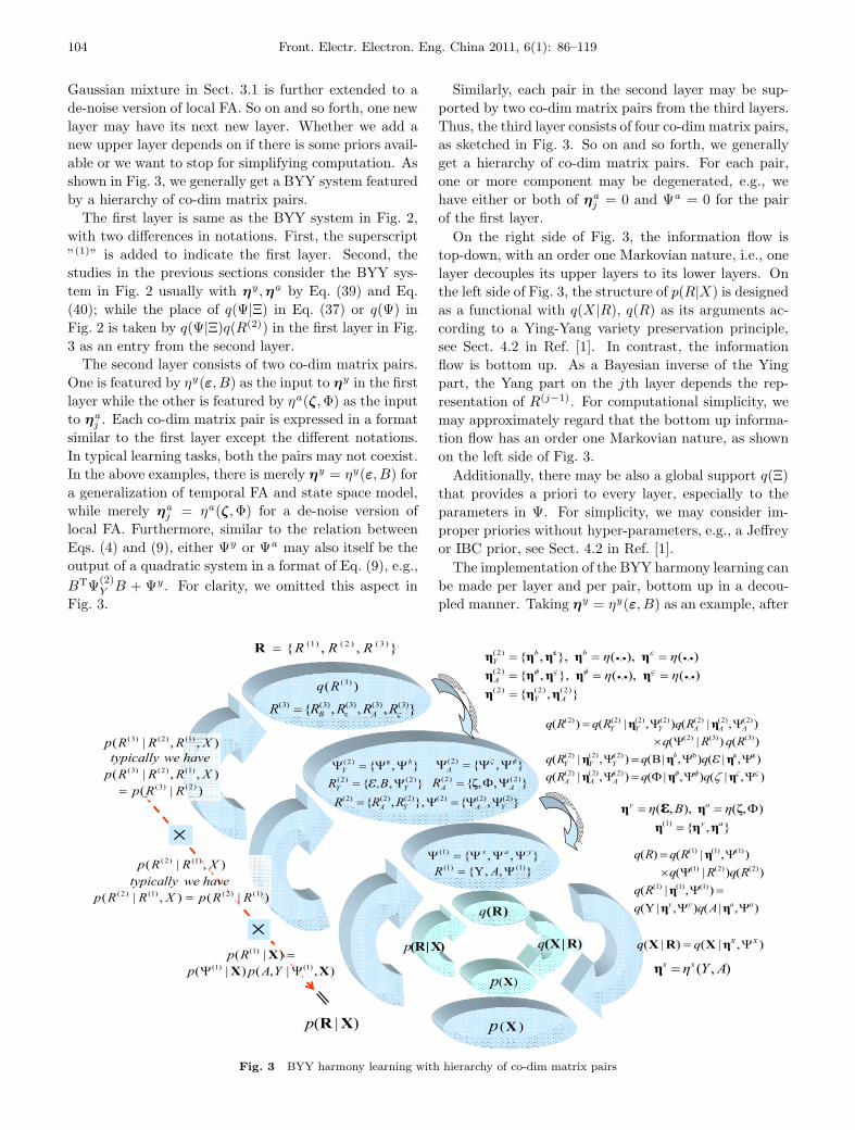
104 Front. Electr. Electron. Eng. China 2011, 6(1): 86–119
Gaussian mixture in Sect. 3.1 is further extended to ade-noise version of local FA. So on and so forth, one newlayer may have its next new layer. Whether we add anew upper layer depends on if there is some priors avail-able or we want to stop for simplifying computation. Asshown in Fig. 3, we generally get a BYY system featuredby a hierarchy of co-dim matrix pairs.
The first layer is same as the BYY system in Fig. 2,with two differences in notations. First, the superscript”(1)” is added to indicate the first layer. Second, thestudies in the previous sections consider the BYY sys-tem in Fig. 2 usually with ηy ,ηa by Eq. (39) and Eq.(40); while the place of q(Ψ|Ξ) in Eq. (37) or q(Ψ) inFig. 2 is taken by q(Ψ|Ξ)q(R(2)) in the first layer in Fig.3 as an entry from the second layer.
The second layer consists of two co-dim matrix pairs.One is featured by ηy(ε, B) as the input to ηy in the firstlayer while the other is featured by ηa(ζ,Φ) as the inputto ηa
j . Each co-dim matrix pair is expressed in a formatsimilar to the first layer except the different notations.In typical learning tasks, both the pairs may not coexist.In the above examples, there is merely ηy = ηy(ε, B) fora generalization of temporal FA and state space model,while merely ηa
j = ηa(ζ,Φ) for a de-noise version oflocal FA. Furthermore, similar to the relation betweenEqs. (4) and (9), either Ψy or Ψa may also itself be theoutput of a quadratic system in a format of Eq. (9), e.g.,BTΨ(2)
Y B + Ψy . For clarity, we omitted this aspect inFig. 3.
Similarly, each pair in the second layer may be sup-ported by two co-dim matrix pairs from the third layers.Thus, the third layer consists of four co-dim matrix pairs,as sketched in Fig. 3. So on and so forth, we generallyget a hierarchy of co-dim matrix pairs. For each pair,one or more component may be degenerated, e.g., wehave either or both of ηa
j = 0 and Ψa = 0 for the pairof the first layer.
On the right side of Fig. 3, the information flow istop-down, with an order one Markovian nature, i.e., onelayer decouples its upper layers to its lower layers. Onthe left side of Fig. 3, the structure of p(R|X) is designedas a functional with q(X |R), q(R) as its arguments ac-cording to a Ying-Yang variety preservation principle,see Sect. 4.2 in Ref. [1]. In contrast, the informationflow is bottom up. As a Bayesian inverse of the Yingpart, the Yang part on the jth layer depends the rep-resentation of R(j−1). For computational simplicity, wemay approximately regard that the bottom up informa-tion flow has an order one Markovian nature, as shownon the left side of Fig. 3.
Additionally, there may be also a global support q(Ξ)that provides a priori to every layer, especially to theparameters in Ψ. For simplicity, we may consider im-proper priories without hyper-parameters, e.g., a Jeffreyor IBC prior, see Sect. 4.2 in Ref. [1].
The implementation of the BYY harmony learning canbe made per layer and per pair, bottom up in a decou-pled manner. Taking ηy = ηy(ε, B) as an example, after
},,{ )3()2()1( RRRR
)|( XRp )(Xp
),|()|( xxqq XRX
),|,()|()|(
)1()1(
)1(
XXXYApp
Rp
)|(),|(
),|(
)1()2()1()2(
)1()2(
RRpXRRpwe havetypically
XRRp
},,,{ )3()3()3()3()3( RRRRR AB
)(Xp
)R(q
)R|X(q)X|R(p
},,Y{},,{
)1()1(
)1(
AR
yax
},{},{)2()2(
)2(
YY
bY
,BR
),|(),|Y(),|(
)()|(),|()(
)1()1()1(
)2()2()1(
)1()1()1(
aayy AqqRq
RqRqRqRq
),( AYxx
},{),(),,(
)1( ay
ay B
),|(),|(),|(),|(),|B(),|()()|(),|(),|()(
)2()2()2(
b)2()2()2(
)3()3()2(
)2()2()2()2()2()2()2(
qqRqqqRq
RqRqRqRqRq
AAA
bYYY
AAAYYY
},,{},{)2()2(
)2(
AA
A
R},{},,{ )2()2()2()2()2()2(
YAYA RRR
)( )3(Rq
)|(),,|(
),,|(
)2()3(
)1()2()3(
)1()2()3(
RRpXRRRp
we havetypicallyXRRRp
},{)(),(},,{)(),(},,{
)2()2()2(
,,)2(
,,)2(
AY
A
bbY
Fig. 3 BYY harmony learning with hierarchy of co-dim matrix pairs
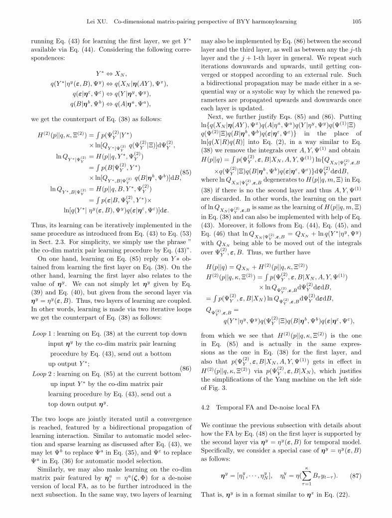
Lei XU. Co-dimensional matrix-pairing perspective of BYY harmonylearning 105
running Eq. (43) for learning the first layer, we get Y ∗
available via Eq. (44). Considering the following corre-spondences:
Y ∗ ⇔ XN ,
q(Y ∗|ηy(ε, B),Ψy) ⇔ q(XN |η(AY ),Ψx ),
q(ε|ηε,Ψε) ⇔ q(Y |ηy ,Ψy),
q(B|ηb ,Ψb) ⇔ q(A|ηa ,Ψa),
we get the counterpart of Eq. (38) as follows:
H(2)(p||q, κ,Ξ(2)) =∫p(Ψ(2)
Y |Y ∗)× ln[Q
Y ∗|Ψ(2)Y
q(Ψ(2)Y |Ξ)]dΨ(2)
Y ,
lnQY ∗|Ψ(2)
Y
= H(p||q, Y ∗,Ψ(2)Y )
=∫p(B|Ψ(2)
Y , Y ∗)
× ln[QY ∗,B|Ψ(2)
Y
q(B|ηb ,Ψb)]dB,
lnQY ∗,B|Ψ(2)
Y
= H(p||q,B, Y ∗,Ψ(2)Y )
=∫p(ε|B,Ψ(2)
Y , Y ∗)×ln[q(Y ∗| ηy(ε, B),Ψy)q(ε|ηε,Ψε)]dε.
(85)
Thus, its learning can be iteratively implemented in thesame procedure as introduced from Eq. (43) to Eq. (53)in Sect. 2.3. For simplicity, we simply use the phrase ”the co-dim matrix pair learning procedure by Eq. (43)”.
On one hand, learning on Eq. (85) reply on Y ∗ ob-tained from learning the first layer on Eq. (38). On theother hand, learning the first layer also relates to thevalue of ηy . We can not simply let ηy given by Eq.(39) and Eq. (40), but given from the second layer viaηy = ηy(ε, B). Thus, two layers of learning are coupled.In other words, learning is made via two iterative loopswe get the counterpart of Eq. (38) as follows:
Loop 1 : learning on Eq. (38) at the current top down
input ηy by the co-dim matrix pair learning
procedure by Eq. (43), send out a bottomup output Y ∗;
Loop 2 : learning on Eq. (85) at the current bottom
up input Y ∗ by the co-dim matrix pair
learning procedure by Eq. (43), send out atop down output ηy .
(86)
The two loops are jointly iterated until a convergenceis reached, featured by a bidirectional propagation oflearning interaction. Similar to automatic model selec-tion and sparse learning as discussed after Eq. (43), wemay let Ψb to replace Ψa in Eq. (35), and Ψε to replaceΨa in Eq. (36) for automatic model selection.
Similarly, we may also make learning on the co-dimmatrix pair featured by ηa
j = ηa(ζ,Φ) for a de-noiseversion of local FA, as to be further introduced in thenext subsection. In the same way, two layers of learning
may also be implemented by Eq. (86) between the secondlayer and the third layer, as well as between any the j-thlayer and the j + 1-th layer in general. We repeat suchiterations downwards and upwards, until getting con-verged or stopped according to an external rule. Sucha bidirectional propagation may be made either in a se-quential way or a systolic way by which the renewed pa-rameters are propagated upwards and downwards onceeach layer is updated.
Next, we further justify Eqs. (85) and (86). Puttingln{q(XN |η(AY ),Ψx )q(A|ηa ,Ψa)q(Y |ηy ,Ψy)q(Ψ(1)|Ξ)q(Ψ(2)|Ξ)q(B|ηb ,Ψb)q(ε|ηε,Ψε)} in the place ofln[q(X |R)q(R)] into Eq. (2), in a way similar to Eq.(38) we remove the integrals over A, Y,Ψ(1) and obtainH(p||q) =
∫p(Ψ(2)
Y , ε, B|XN , A, Y,Ψ(1)) ln{QXN |Ψ(2)
Y ,ε,B
×q(Ψ(2)Y |Ξ)q(B|ηb ,Ψb)q(ε|ηε,Ψε)}dΨ(2)
Y dεdB,where lnQ
XN |Ψ(2)Y ,ε,B
degenerates toH(p||q,m,Ξ) in Eq.
(38) if there is no the second layer and thus A, Y,Ψ(1)
are discarded. In other words, the learning on the partof lnQ
XN |Ψ(2)Y ,ε,B
is same as the learning ofH(p||q,m,Ξ)in Eq. (38) and can also be implemented with help of Eq.(43). Moreover, it follows from Eq. (44), Eq. (45), andEq. (46) that lnQ
XN |Ψ(2)Y ,ε,B
= QXN + ln q(Y ∗|ηy ,Ψy)with QXN being able to be moved out of the integralsover Ψ(2)
Y , ε, B. Thus, we further have
H(p||q) = QXN +H(2)(p||q, κ,Ξ(2))
H(2)(p||q, κ,Ξ(2)) =∫p(Ψ(2)
Y , ε, B|XN , A, Y,Ψ(1))
× lnQΨ
(2)Y ,ε,B
dΨ(2)Y dεdB,
=∫p(Ψ(2)
Y , ε, B|XN) lnQΨ
(2)Y ,ε,B
dΨ(2)Y dεdB,
QΨ
(2)Y ,ε,B
=
q(Y ∗|ηy ,Ψy)q(Ψ(2)Y |Ξ)q(B|ηb ,Ψb)q(ε|ηε,Ψε),
from which we see that H(2)(p||q, κ,Ξ(2)) is the onein Eq. (85) and is actually in the same expres-sions as the one in Eq. (38) for the first layer, andalso that p(Ψ(2)
Y , ε, B|XN , A, Y,Ψ(1)) gets in effect inH(2)(p||q, κ,Ξ(2)) via p(Ψ(2)
Y , ε, B|XN ), which justifiesthe simplifications of the Yang machine on the left sideof Fig. 3.
4.2 Temporal FA and De-noise local FA
We continue the previous subsection with details abouthow the FA by Eq. (48) on the first layer is supported bythe second layer via ηy = ηy(ε, B) for temporal model.Specifically, we consider a special case of ηy = ηy(ε, B)as follows:
ηy = [ηy1 , · · · , ηyN ], ηyt = η(κ∑τ=1
Bτyt−τ ). (87)
That is, ηy is in a format similar to ηx in Eq. (22).
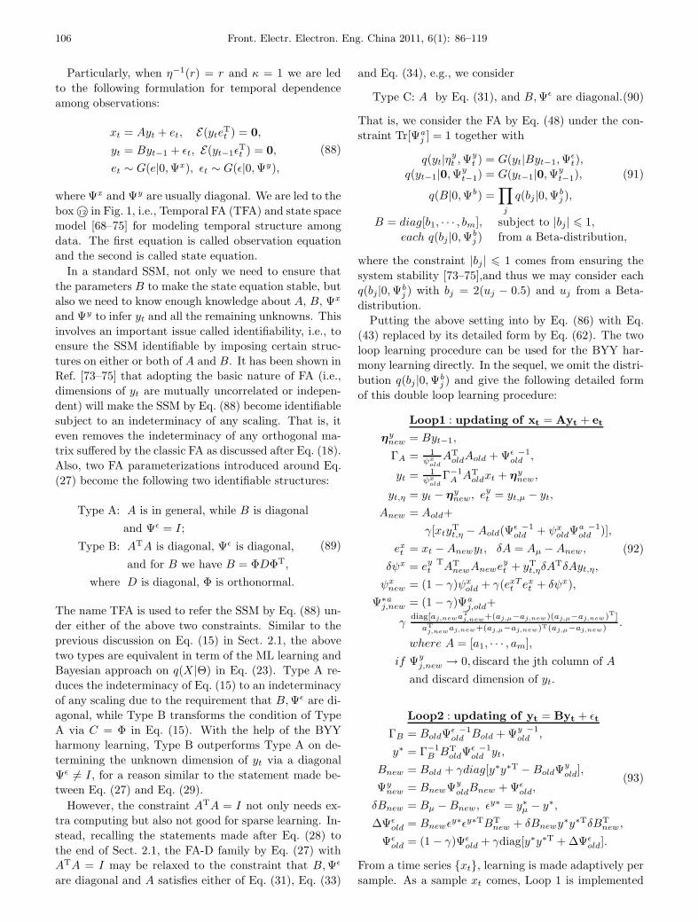
106 Front. Electr. Electron. Eng. China 2011, 6(1): 86–119
Particularly, when η−1(r) = r and κ = 1 we are ledto the following formulation for temporal dependenceamong observations:
xt = Ayt + et, E(yteTt ) = 0,
yt = Byt−1 + εt, E(yt−1εTt ) = 0,
et ∼ G(e|0,Ψx ), εt ∼ G(ε|0,Ψy),
(88)
where Ψx and Ψy are usually diagonal. We are led to thebox 12© in Fig. 1, i.e., Temporal FA (TFA) and state spacemodel [68–75] for modeling temporal structure amongdata. The first equation is called observation equationand the second is called state equation.
In a standard SSM, not only we need to ensure thatthe parameters B to make the state equation stable, butalso we need to know enough knowledge about A, B, Ψx
and Ψy to infer yt and all the remaining unknowns. Thisinvolves an important issue called identifiability, i.e., toensure the SSM identifiable by imposing certain struc-tures on either or both of A and B. It has been shown inRef. [73–75] that adopting the basic nature of FA (i.e.,dimensions of yt are mutually uncorrelated or indepen-dent) will make the SSM by Eq. (88) become identifiablesubject to an indeterminacy of any scaling. That is, iteven removes the indeterminacy of any orthogonal ma-trix suffered by the classic FA as discussed after Eq. (18).Also, two FA parameterizations introduced around Eq.(27) become the following two identifiable structures:
Type A: A is in general, while B is diagonal
and Ψε = I;
Type B: ATA is diagonal, Ψε is diagonal,
and for B we have B = ΦDΦT,
where D is diagonal, Φ is orthonormal.
(89)
The name TFA is used to refer the SSM by Eq. (88) un-der either of the above two constraints. Similar to theprevious discussion on Eq. (15) in Sect. 2.1, the abovetwo types are equivalent in term of the ML learning andBayesian approach on q(X |Θ) in Eq. (23). Type A re-duces the indeterminacy of Eq. (15) to an indeterminacyof any scaling due to the requirement that B,Ψε are di-agonal, while Type B transforms the condition of TypeA via C = Φ in Eq. (15). With the help of the BYYharmony learning, Type B outperforms Type A on de-termining the unknown dimension of yt via a diagonalΨε �= I, for a reason similar to the statement made be-tween Eq. (27) and Eq. (29).
However, the constraint ATA = I not only needs ex-tra computing but also not good for sparse learning. In-stead, recalling the statements made after Eq. (28) tothe end of Sect. 2.1, the FA-D family by Eq. (27) withATA = I may be relaxed to the constraint that B,Ψε
are diagonal and A satisfies either of Eq. (31), Eq. (33)
and Eq. (34), e.g., we consider
Type C: A by Eq. (31), and B,Ψε are diagonal.(90)
That is, we consider the FA by Eq. (48) under the con-straint Tr[Ψa
j ] = 1 together with
q(yt|ηyt ,Ψyt ) = G(yt|Byt−1,Ψε
t),q(yt−1|0,Ψy
t−1) = G(yt−1|0,Ψyt−1), (91)
q(B|0,Ψb) =∏j
q(bj|0,Ψbj ),
B = diag[b1, · · · , bm], subject to |bj | � 1,each q(bj |0,Ψb
j ) from a Beta-distribution,
where the constraint |bj| � 1 comes from ensuring thesystem stability [73–75],and thus we may consider eachq(bj|0,Ψb
j ) with bj = 2(uj − 0.5) and uj from a Beta-distribution.
Putting the above setting into by Eq. (86) with Eq.(43) replaced by its detailed form by Eq. (62). The twoloop learning procedure can be used for the BYY har-mony learning directly. In the sequel, we omit the distri-bution q(bj |0,Ψb
j ) and give the following detailed formof this double loop learning procedure:
Loop1 : updating of xt = Ayt + et
ηynew = Byt−1,
ΓA = 1ψx
oldAToldAold + Ψε −1
old ,
yt = 1ψx
oldΓ−1A AT
oldxt + ηynew,
yt,η = yt − ηynew, e
yt = yt,μ − yt,
Anew = Aold+γ[xtyT
t,η −Aold(Ψε −1old + ψxoldΨ
a −1old )],
ext = xt −Anewyt, δA = Aμ −Anew ,
δψx = ey Tt AT
newAneweyt + yT
t,ηδATδAyt,η,
ψxnew = (1 − γ)ψx
old + γ(exTt ext + δψx ),Ψ∗aj,new = (1 − γ)Ψa
j,old+
γdiag[aj,newa
Tj,new+(aj,μ−aj,new)(aj,μ−aj,new)T]
aTj,newaj,new+(aj,μ−aj,new)T(aj,μ−aj,new)
.
where A = [a1, · · · , am],
if Ψyj,new → 0, discard the jth column of A
and discard dimension of yt.
(92)
Loop2 : updating of yt = Byt + εt
ΓB = BoldΨε −1old Bold + Ψy −1
old ,
y∗ = Γ−1B BT
oldΨε −1old yt,
Bnew = Bold + γdiag[y∗y∗T −BoldΨyold],
Ψynew = BnewΨy
oldBnew + Ψεold,
δBnew = Bμ −Bnew , εy∗ = y∗μ − y∗,
ΔΨεold = Bnewε
y∗εy∗TBTnew + δBnewy
∗y∗TδBTnew ,
Ψεold = (1 − γ)Ψε
old + γdiag[y∗y∗T + ΔΨεold].
(93)
From a time series {xt}, learning is made adaptively persample. As a sample xt comes, Loop 1 is implemented
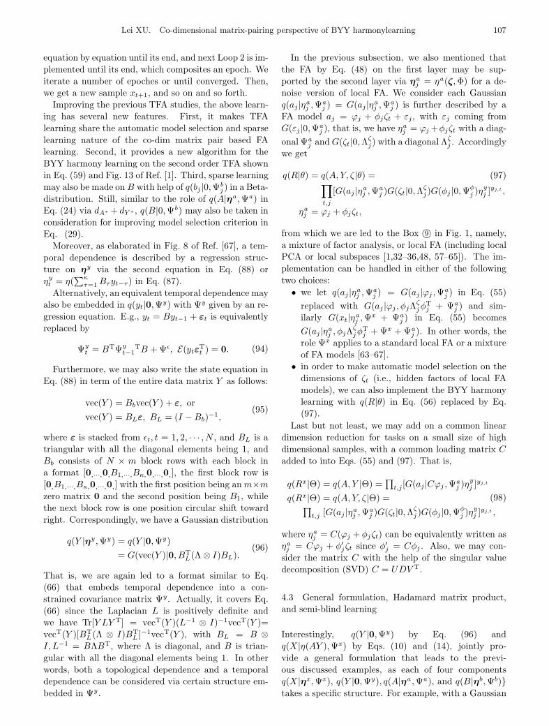
Lei XU. Co-dimensional matrix-pairing perspective of BYY harmonylearning 107
equation by equation until its end, and next Loop 2 is im-plemented until its end, which composites an epoch. Weiterate a number of epoches or until converged. Then,we get a new sample xt+1, and so on and so forth.
Improving the previous TFA studies, the above learn-ing has several new features. First, it makes TFAlearning share the automatic model selection and sparselearning nature of the co-dim matrix pair based FAlearning. Second, it provides a new algorithm for theBYY harmony learning on the second order TFA shownin Eq. (59) and Fig. 13 of Ref. [1]. Third, sparse learningmay also be made on B with help of q(bj |0,Ψb
j ) in a Beta-distribution. Still, similar to the role of q(A|ηa ,Ψa) inEq. (24) via dA∗ + dY ∗ , q(B|0,Ψb) may also be taken inconsideration for improving model selection criterion inEq. (29).
Moreover, as elaborated in Fig. 8 of Ref. [67], a tem-poral dependence is described by a regression struc-ture on ηy via the second equation in Eq. (88) orηyt = η(
∑κτ=1Bτyt−τ ) in Eq. (87).
Alternatively, an equivalent temporal dependence mayalso be embedded in q(yt|0,Ψy) with Ψy given by an re-gression equation. E.g., yt = Byt−1 + εt is equivalentlyreplaced by
Ψyt = BTΨy
t−1TB + Ψε, E(ytεT
t ) = 0. (94)
Furthermore, we may also write the state equation inEq. (88) in term of the entire data matrix Y as follows:
vec(Y ) = Bbvec(Y ) + ε, or
vec(Y ) = BLε, BL = (I −Bb)−1,(95)
where ε is stacked from εt, t = 1, 2, · · · , N , and BL is atriangular with all the diagonal elements being 1, andBb consists of N × m block rows with each block ina format [0,···,0,B1,···,Bκ,0,···,0,], the first block row is[0,B1,···,Bκ,0,···,0,] with the first position being anm×mzero matrix 0 and the second position being B1, whilethe next block row is one position circular shift towardright. Correspondingly, we have a Gaussian distribution
q(Y |ηy ,Ψy) = q(Y |0,Ψy)= G(vec(Y )|0, BT
L(Λ ⊗ I)BL).(96)
That is, we are again led to a format similar to Eq.(66) that embeds temporal dependence into a con-strained covariance matrix Ψy . Actually, it covers Eq.(66) since the Laplacian L is positively definite andwe have Tr[Y LY T] = vecT(Y )(L−1 ⊗ I)−1vecT(Y )=vecT(Y )[BT
L (Λ ⊗ I)BTL ]−1vecT(Y ), with BL = B ⊗
I, L−1 = BΛBT, where Λ is diagonal, and B is trian-gular with all the diagonal elements being 1. In otherwords, both a topological dependence and a temporaldependence can be considered via certain structure em-bedded in Ψy .
In the previous subsection, we also mentioned thatthe FA by Eq. (48) on the first layer may be sup-ported by the second layer via ηa
j = ηa(ζ,Φ) for a de-noise version of local FA. We consider each Gaussianq(aj |ηaj ,Ψa
j ) = G(aj |ηaj ,Ψaj ) is further described by a
FA model aj = ϕj + φjζt + εj , with εj coming fromG(εj |0,Ψa
j ), that is, we have ηaj = ϕj+φjζt with a diag-onal Ψa
j andG(ζt|0,Λζj) with a diagonal Λζj . Accordinglywe get
q(R|θ) = q(A, Y, ζ|θ) = (97)∏t,j
[G(aj |ηaj ,Ψaj )G(ζt|0,Λζj)G(φj |0,Ψφ
j )ηyj ]yj,t ,
ηaj = ϕj + φjζt,
from which we are led to the Box 9© in Fig. 1, namely,a mixture of factor analysis, or local FA (including localPCA or local subspaces [1,32–36,48, 57–65]). The im-plementation can be handled in either of the followingtwo choices:
• we let q(aj |ηaj ,Ψaj ) = G(aj |ϕj ,Ψa
j ) in Eq. (55)replaced with G(aj |ϕj , φjΛζjφT
j + Ψaj ) and sim-
ilarly G(xt|ηaj ,Ψx + Ψaj ) in Eq. (55) becomes
G(aj |ηaj , φjΛζjφTj + Ψx + Ψa
j ). In other words, therole Ψx applies to a standard local FA or a mixtureof FA models [63–67].
• in order to make automatic model selection on thedimensions of ζt (i.e., hidden factors of local FAmodels), we can also implement the BYY harmonylearning with q(R|θ) in Eq. (56) replaced by Eq.(97).
Last but not least, we may add on a common lineardimension reduction for tasks on a small size of highdimensional samples, with a common loading matrix Cadded to into Eqs. (55) and (97). That is,
q(Rx |Θ) = q(A, Y |Θ) =∏t,j [G(aj |Cϕj ,Ψa
j )ηyj ]yj,t
q(Rx |Θ) = q(A, Y, ζ|Θ) =∏t,j [G(aj |ηaj ,Ψa
j )G(ζt|0,Λζj )G(φj |0,Ψφj )η
yj ]yj,t ,
(98)
where ηaj = C(ϕj + φjζt) can be equivalently written asηaj = Cϕj + φ′jζt since φ′j = Cφj . Also, we may con-sider the matrix C with the help of the singular valuedecomposition (SVD) C = UDV T.
4.3 General formulation, Hadamard matrix product,and semi-blind learning
Interestingly, q(Y |0,Ψy) by Eq. (96) andq(X |η(AY ),Ψx ) by Eqs. (10) and (14), jointly pro-vide a general formulation that leads to the previ-ous discussed examples, as each of four componentsq(X |ηx,Ψx), q(Y |0,Ψy), q(A|ηa ,Ψa), and q(B|ηb,Ψb)}takes a specific structure. For example, with a Gaussian
108 Front. Electr. Electron. Eng. China 2011, 6(1): 86–119
q(X |AY,Ψx ) we have
X = AY + E, vec[Y ] = μy +BLε. (99)
That is, Y can be regarded as generated from ε via alinear mapping BL by a sparse matrix with its nonzeroparameters coming from nonzero parameters of B in aspecific structure.
For an efficient implementation we usually return tothe task motivated original models, such as Eq. (66) formanifold learning and Eq. (88) for TFA, in order toavoid a huge dimensional problem of BL. Even so, theequation vec(Y ) = μy + BLε not only provides con-ceptually a unified expression for variance dependencestructures among Y , but also motivates further issues toinvestigate:
• Beyond a Gaussian q(X |ηx ,Ψx ) and a Gaussianq(Y |ηy ,Ψy), Eq. (96) can be extended to an evengeneral form with q(X |ηx ,Ψx ), q(Y |ηy ,Ψy) givenby Eq. (10) while ηx , ηy given by Eq. (22) withη(r) taking one of typical choices shown in Table 1.
• The linear model by Eq. (4) is a common part ofvarious data generating models, while the secondpart vec(Y ) = μy +BLε should be considered basedcertain intrinsic properties of problems. Moreover,BLε may also be extended to nonlinear mapping.
• This general guide is also helpful to making specificinvestigation. E.g., to check whether the LaplacianL from X by Eq. (66) preserves the topology under-lying the one introduced by BL, we may examine
whether the cascaded mapping ABL preserves thistopology.
As discussed after Eq. (99), BL is generally in a sparsestructure. Recalling Eq. (70), we may encode a sparsematrix with help of binary variables that controls sparsedegree and flexibly accommodates different matrix struc-tures. Integrating Eq. (70) with the sate space model byEq. (88), we further proceed to the following binary vari-able modulated state space model:
X = (A ◦ LA)Y + E,
A ◦ LA = [aij�aij ],
vec(Y ) = μy + (B ◦ LB)ε,B ◦ LB = [bij�bij ].
(100)
As shown in Fig.4 and also illustrated by the Box 17© inFig. 1, we get a general formulation for semi-blind learn-ing. The first layer co-dim matrix pair ηx = AY getsone second layer support A◦LA in a Hadamard productfor modulating A, and the other second layer supportμy + Bε in an ordinary matrix product for modulatingY . Then, B in the second layer is further modulated bya third layer support B ◦ LB in a Hadamard product.Following the two formations of semi-blind learning byEq. (70) and Eq. (71), letting B = 0 in Eq. (100) leadsto the third formation of semi-blind learning that can beregarded as an extension of NCA [76–79], as illustratedin the Box 16© in Fig. 1.
md
N
X AL LAA
][ ,tiyY
d
d ][ aijijA aLA
linked.not0,linked,,1a
ij
m
m N
}{ ,ti
ttBt yLBy1 , )(ttAt eyLAx )(
][ ,,,bijijB bLB
linked.not0,linked,,1
,bij
Y
][ ijaA][ a
ijAL ][ ,,bijBL
][ ,ijbB
}.,,,{ with),,|()X|Y,,,,,()()|()()()(),|(),|(),|Y(),|X()()|(
]ln[
2BA
yxNN
BBAAyyxx
N
IhXXGABpXpXRpqqqBqAqqqRqRXq
dRdXq(X|R)q(R)p(R|X)p(X)H(p||q)
Fig. 4 General formulation, sparse learning, and semi-blind learning
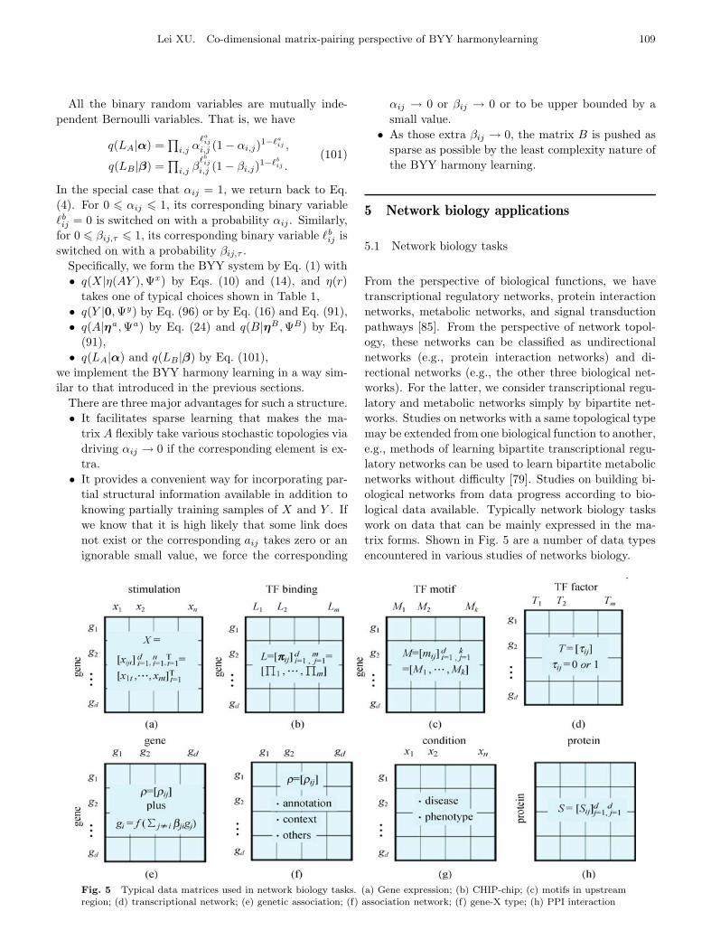
Lei XU. Co-dimensional matrix-pairing perspective of BYY harmonylearning 109
All the binary random variables are mutually inde-pendent Bernoulli variables. That is, we have
q(LA|α) =∏i,j α
aij
i,j (1 − αi,j)1−aij ,
q(LB|β) =∏i,j β
bij
i,j (1 − βi,j)1−bij .
(101)
In the special case that αij = 1, we return back to Eq.(4). For 0 � αij � 1, its corresponding binary variable�bij = 0 is switched on with a probability αij . Similarly,for 0 � βij,τ � 1, its corresponding binary variable �bij isswitched on with a probability βij,τ .
Specifically, we form the BYY system by Eq. (1) with• q(X |η(AY ),Ψx ) by Eqs. (10) and (14), and η(r)
takes one of typical choices shown in Table 1,• q(Y |0,Ψy) by Eq. (96) or by Eq. (16) and Eq. (91),• q(A|ηa ,Ψa) by Eq. (24) and q(B|ηB,ΨB) by Eq.
(91),• q(LA|α) and q(LB|β) by Eq. (101),
we implement the BYY harmony learning in a way sim-ilar to that introduced in the previous sections.
There are three major advantages for such a structure.• It facilitates sparse learning that makes the ma-
trix A flexibly take various stochastic topologies viadriving αij → 0 if the corresponding element is ex-tra.
• It provides a convenient way for incorporating par-tial structural information available in addition toknowing partially training samples of X and Y . Ifwe know that it is high likely that some link doesnot exist or the corresponding aij takes zero or anignorable small value, we force the corresponding
αij → 0 or βij → 0 or to be upper bounded by asmall value.
• As those extra βij → 0, the matrix B is pushed assparse as possible by the least complexity nature ofthe BYY harmony learning.
5 Network biology applications
5.1 Network biology tasks
From the perspective of biological functions, we havetranscriptional regulatory networks, protein interactionnetworks, metabolic networks, and signal transductionpathways [85]. From the perspective of network topol-ogy, these networks can be classified as undirectionalnetworks (e.g., protein interaction networks) and di-rectional networks (e.g., the other three biological net-works). For the latter, we consider transcriptional regu-latory and metabolic networks simply by bipartite net-works. Studies on networks with a same topological typemay be extended from one biological function to another,e.g., methods of learning bipartite transcriptional regu-latory networks can be used to learn bipartite metabolicnetworks without difficulty [79]. Studies on building bi-ological networks from data progress according to bio-logical data available. Typically network biology taskswork on data that can be mainly expressed in the ma-trix forms. Shown in Fig. 5 are a number of data typesencountered in various studies of networks biology.
Fig. 5 Typical data matrices used in network biology tasks. (a) Gene expression; (b) CHIP-chip; (c) motifs in upstreamregion; (d) transcriptional network; (e) genetic association; (f) association network; (f) gene-X type; (h) PPI interaction
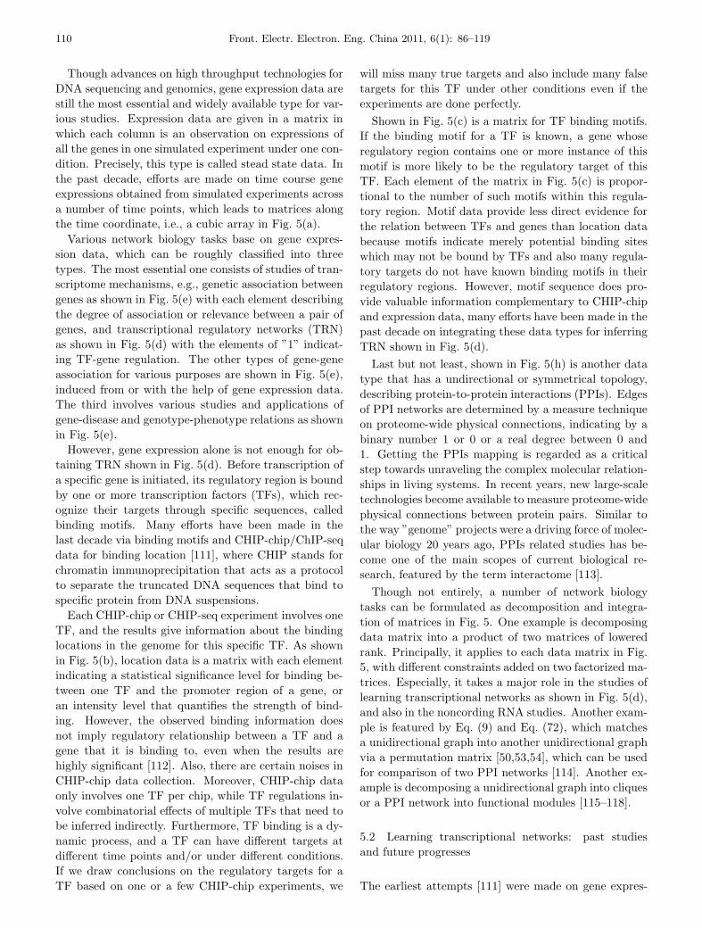
110 Front. Electr. Electron. Eng. China 2011, 6(1): 86–119
Though advances on high throughput technologies forDNA sequencing and genomics, gene expression data arestill the most essential and widely available type for var-ious studies. Expression data are given in a matrix inwhich each column is an observation on expressions ofall the genes in one simulated experiment under one con-dition. Precisely, this type is called stead state data. Inthe past decade, efforts are made on time course geneexpressions obtained from simulated experiments acrossa number of time points, which leads to matrices alongthe time coordinate, i.e., a cubic array in Fig. 5(a).
Various network biology tasks base on gene expres-sion data, which can be roughly classified into threetypes. The most essential one consists of studies of tran-scriptome mechanisms, e.g., genetic association betweengenes as shown in Fig. 5(e) with each element describingthe degree of association or relevance between a pair ofgenes, and transcriptional regulatory networks (TRN)as shown in Fig. 5(d) with the elements of ”1” indicat-ing TF-gene regulation. The other types of gene-geneassociation for various purposes are shown in Fig. 5(e),induced from or with the help of gene expression data.The third involves various studies and applications ofgene-disease and genotype-phenotype relations as shownin Fig. 5(e).
However, gene expression alone is not enough for ob-taining TRN shown in Fig. 5(d). Before transcription ofa specific gene is initiated, its regulatory region is boundby one or more transcription factors (TFs), which rec-ognize their targets through specific sequences, calledbinding motifs. Many efforts have been made in thelast decade via binding motifs and CHIP-chip/ChIP-seqdata for binding location [111], where CHIP stands forchromatin immunoprecipitation that acts as a protocolto separate the truncated DNA sequences that bind tospecific protein from DNA suspensions.
Each CHIP-chip or CHIP-seq experiment involves oneTF, and the results give information about the bindinglocations in the genome for this specific TF. As shownin Fig. 5(b), location data is a matrix with each elementindicating a statistical significance level for binding be-tween one TF and the promoter region of a gene, oran intensity level that quantifies the strength of bind-ing. However, the observed binding information doesnot imply regulatory relationship between a TF and agene that it is binding to, even when the results arehighly significant [112]. Also, there are certain noises inCHIP-chip data collection. Moreover, CHIP-chip dataonly involves one TF per chip, while TF regulations in-volve combinatorial effects of multiple TFs that need tobe inferred indirectly. Furthermore, TF binding is a dy-namic process, and a TF can have different targets atdifferent time points and/or under different conditions.If we draw conclusions on the regulatory targets for aTF based on one or a few CHIP-chip experiments, we
will miss many true targets and also include many falsetargets for this TF under other conditions even if theexperiments are done perfectly.
Shown in Fig. 5(c) is a matrix for TF binding motifs.If the binding motif for a TF is known, a gene whoseregulatory region contains one or more instance of thismotif is more likely to be the regulatory target of thisTF. Each element of the matrix in Fig. 5(c) is propor-tional to the number of such motifs within this regula-tory region. Motif data provide less direct evidence forthe relation between TFs and genes than location databecause motifs indicate merely potential binding siteswhich may not be bound by TFs and also many regula-tory targets do not have known binding motifs in theirregulatory regions. However, motif sequence does pro-vide valuable information complementary to CHIP-chipand expression data, many efforts have been made in thepast decade on integrating these data types for inferringTRN shown in Fig. 5(d).
Last but not least, shown in Fig. 5(h) is another datatype that has a undirectional or symmetrical topology,describing protein-to-protein interactions (PPIs). Edgesof PPI networks are determined by a measure techniqueon proteome-wide physical connections, indicating by abinary number 1 or 0 or a real degree between 0 and1. Getting the PPIs mapping is regarded as a criticalstep towards unraveling the complex molecular relation-ships in living systems. In recent years, new large-scaletechnologies become available to measure proteome-widephysical connections between protein pairs. Similar tothe way ”genome” projects were a driving force of molec-ular biology 20 years ago, PPIs related studies has be-come one of the main scopes of current biological re-search, featured by the term interactome [113].
Though not entirely, a number of network biologytasks can be formulated as decomposition and integra-tion of matrices in Fig. 5. One example is decomposingdata matrix into a product of two matrices of loweredrank. Principally, it applies to each data matrix in Fig.5, with different constraints added on two factorized ma-trices. Especially, it takes a major role in the studies oflearning transcriptional networks as shown in Fig. 5(d),and also in the noncording RNA studies. Another exam-ple is featured by Eq. (9) and Eq. (72), which matchesa unidirectional graph into another unidirectional graphvia a permutation matrix [50,53,54], which can be usedfor comparison of two PPI networks [114]. Another ex-ample is decomposing a unidirectional graph into cliquesor a PPI network into functional modules [115–118].
5.2 Learning transcriptional networks: past studiesand future progresses
The earliest attempts [111] were made on gene expres-
Lei XU. Co-dimensional matrix-pairing perspective of BYY harmonylearning 111
sion data in Fig. 5(a) alone. The inferred networks con-sider general relationships among genes, and thus shouldbe more appropriately named as gene regulatory net-works. A fundamental limitation is the assumption thatthe expression levels of genes depend on the expressionlevels of the TFs regulating those genes. Expression dataonly measures the mRNA abundances, while it is the TFproteins that are directly involved in the regulation ofgenes. The mRNA levels of the TFs may not be highlycorrelated with those of the genes they regulate. In thepast decade, progresses have been obtained on study-ing transcriptional regulation networks (TRN) with thehelp of location data shown in Fig. 4(b). The task isfeatured by finding the bipartite networks expressed bythe binary matrix in Fig. 5(d). The effort starts fromgetting bipartite networks for TRN, which may also bebacktracked by three streams.
One stream is featured by bi-clustering that groupsgenes and their corresponding TFs into functional mod-ules. Genes in the same module exhibit similar expres-sion profiles and tend to have similar biological func-tions. Also, these genes should share similar regulationpatterns and thus are more likely to be under the controlof the similar TFs. This bi-clustering bases both the sim-ilarities of expression profiles and the activities of TFs.In the absence of information for TF activities, Segal etal. [119] infers key TFs of each module by correlating thegene expression levels with expression patterns of genesin the module across a large number of experimental con-ditions, and then the obtained TFs activities and geneexpression data are jointly used to accurately assign eachgene to its corresponding module. Inferring key TFs andmaking clustering are made iteratively. However, thisprocedure is limited by the possibly poor correspondencebetween gene expression levels and TF activities. Reisset al. [120] categorized genes into co-regulated groupsacross a subset of all observed experimental conditionswith the help of bi-clustering (genes and conditions) in-stead of a standard clustering that participates genesinto co-expressed groups. Co-regulated genes are oftenfunctionally associated and easy to be incorporated witha priori such as common cis-regulatory motifs.
Bar-Joseph et al. [112] proposed a procedure calledGRAM that uses the CHIP-chip location data in Fig.5(b) also in a two step iteration. First, a stringentcriterion infers the binding targets only for those TF-gene pairs that have high statistical significance. Sec-ond, gene expression are used to define a core expressionprofile for a set of genes sharing a common set of TFsas their regulators. After the core expression profilesare defined, other genes are included in a transcriptionmodule if their expression profiles are similar to the coreprofiles. Sharing a similar structure, the ReModiscoveryalgorithm by Lemmens et al. [121] uses both the loca-tion data in Fig. 5(b) and the motif data in Fig. 5(c)
to jointly detect modules of tightly co-expressed genesthat share common subsets of TFs and motifs that ex-ceed thresholds. Recently, LeTICE by Youn et al. [122]further extends these studies into a probabilistic modelfor a binary binding matrix for integrating the expres-sion and location data in Fig. 5(a) and 5(b). Withoutrequiring thresholds, LeTICE generates all gene mod-ules simultaneously using the entire set of TFs, insteadof step-wisely getting gene modules via subsets of TFs.
The second stream considers the matrix decomposi-tion by Eq. (4) as bipartite networks, which is justifiedfrom the fact that the equilibrium state of a nonlinearkinetics model leads to that the log-ratio of gene ex-pression levels between two conditions is related to theadditive effects from a set of TFs through the log-ratioof the TF activities to the regulatory strength. Again,early studies began with only gene expression data asX in Eq. (4), one is the singular value decomposition(SVD) [123–127], another is the independent componentanalysis (ICA) [128,129] on the assumption of E = 0.However, the interpretability of SVD and ICA solutionsare a concern. This stems from the fact that orthogonal-ity and statistical independence lack physical meaning.Also, both SVD and ICA assume that the bipartite net-work topology is fully connected, and each source signalcontributes to every output. This is an inappropriateassumption for transcriptional regulation where it is ac-cepted that transcription networks are generally sparse.
Similarly, this stream also moved to considering thesequence data and CHIP-chip location data in Fig. 5(b)and 5(c). Liao et al. [76] considered a prior knowl-edge on the connectivity between TFs and genes butdoes not need knowing regulatory strengths or TF ac-tivities, from which each element of A is set to be zeroif there is no connectivity that corresponds to this ele-ment. With this constraint, the decomposition of Eq.(4) is made via minimizing the Frobenius norm of E todetermine those unknown regulatory strengths, underthe name of network component analysis (NCA). Thisidea is followed and further extended, by Boulesteix andStrimmer [77] with the help of the partial least squaresto reduce the dimensionality of the space spanned by theTFs, by Brynildsen et al. [78] with the help of the Gibssampler to screen for genes with consistent expressionand CHIP-chip derived connectivity data, and also byBrynildsen et al. [79] with the assumption relaxed to benothing about the nature of the source signals beyondlinear independency. Being different from directly us-ing the binding intensities bij from CHIP-chip data, i.e.,aij = bij , Sun et al. [130] assumed that aij = bijcij ,where cij is the unknown but desired regulatory rela-tionship between TF j and gene i. There are also sev-eral other efforts on learning TRN by integrating geneexpression, CHIP-chip, and sequence information [131–133]. Despite different motivations, these methods all
112 Front. Electr. Electron. Eng. China 2011, 6(1): 86–119
share the same general modeling form. Pournara andWernisch [134] compared some methods in this context.
The third stream consists of state space model (SSM)based studies for time course gene expressions across anumber of time points. Gene expression in a generalsituation as shown in Fig. 5(a) is a cubic array thatvaries along three coordinates. It is known that networkfunctions are determined not only by their static struc-tures but also by their dynamic structural rearrange-ments [135]. In recent years, SSM has been adopted fortime course gene expressions. Most of existing studies[136–145] treat data xj,t from j = 1, 2, · · · , n as multi-ple observation series from one same underlying SSM.In Ref. [146], apparently it considers multiple condi-tions with one subscript corresponding explicitly to eachdifferent condition, actually it still considers a sameset of parameters for their SSM across all the condi-tions and thus bring no difference. In these situations,xj,t, j = 1, 2, · · · , n can be equivalently regarded as seg-ments of a same stochastic process. For notation clarity,we ignore the subscript j = 1, 2, · · · , n and simply con-sider a time series X = {xt, t = 1, 2, · · · , T } with eachvector xt that consists of expressions of all the genes.
Two early studies [136,137] proposed to use a so-calledinput driven SSM, i.e., adding an extra term Cxt−1 toboth the state equation and observation equation in astandard SSM by Eq. (88). Later on, most of efforts[138–146] turned back to a standard SSM because ithas been shown that the additional term Cxt−1 basi-cally has no help and may even cause instability [143].Likely, such an input driven term has not been includedin a standard SSM during the past extensive studies [68]just because of an awareness of its useless. Generally,one major SSM problem is the lack of identifiability, forwhich extra structural constraints have been imposed tosolve the problem. In addition to the usual assumptionon et and εt, extra constraints are imposed also on ei-ther or both of A and B. Mostly, A is imposed to bean identity matrix I [144] or its permutation [138,141]or a diagonal matrix [143]. These over-simplified SSMstudies actually work as a filter to removing noises ingene expression data.
Also, this stream recently turns to integrating CHIP-chip and sequence data into the SSM modeling. San-guinetti et al. [138] adopted the sparsity constraint onA in a same way as made in NCA [76], which can beregarded as an extension of NCA into SSM. Similarlybut with more assumptions, constrained SSMs are sug-gested in [140] and [144], also based on a known networkstructure. If a pair of genes is represented by two statesthat is known to have no interaction, the correspondingentry in the matrix B are all set to be zero. Similarly, ifan input has no influence on a gene that is representedas a state, the corresponding entry in A should be zero.
The above overview sketched an outline of frontier
tasks, which motivates to apply the general formulationshown in Fig. 4 for modeling TRN with the help of theBYY harmony learning, with the following advantagesand improvements:
1) As addressed above, imposing that A = I [145] orits permutation [138,141] or that A is diagonal [144] ac-tually makes the role of SSM degenerated to a filter forobservation noises. This limitation can be removed byconsidering the TFA by Eq. (88), which has been shownto be identifiable with the help of either of three struc-tural constraints given by Eq. (89) and Eq. (90).
2) Sanguinetti et al.[138] handled the above limitationby adopting the sparsity on A as used by NCA [76]. Butit is unreliable to simply decide whether or not remove anedge based on the information from sequence data andCHIP-chip location data, as previously introduced. Theformulation in Fig. 4 differs in not only considering ei-ther of the above two types of structural constraints, butalso providing a flexible venue to accommodate stochas-tic topologies to adopt an appropriate one, controlled bythe probability αij obtained from combining the data inFig. 5(b) and 5(c), e.g.,
αij = (1 − γ)πij + γ/(1 + e−mij ), 0 � γ � 1,
where γ controls the proportions of two types of data,which may be pre-specified or obtained via learning.
3) Being different from the existing SSM studies, theprobabilistic sparsity is also imposed on both the obser-vation equation and the state equation by the formu-lation in Fig. 4. With the help of learning each prob-ability 0 � βij � 1, the sparsity of the matrix B isdetermined by the least complexity nature of the BYYharmony learning, in order to learn both the underlyingdynamics of each TF and the relationship across differ-ent TFs.
4) Though the recently proposed LeTICE [122] im-proves the previous studies by using a probabilistic spar-sity on the matrix A also by the Bernoulli binary vari-able, it actually considers merely the first layer in Fig. 4,without considering temporal dependence by the stateequation. That is, it not a SSM modeling, but just abipartite TRN network that uses this probabilistic spar-sity to improve the one used in NCA [76]. In addition,the formulation in Fig. 4 also differs in not only imple-menting the BYY harmony learning but also consideringboth CHIP-chip and sequence information in Fig. 5(b)and 5(c), while LeTICE only considers the CHIP-chipdata in Fig. 5(b).
5) With the help of automatic model selection, thelower rank of the matrix A or equivalently an appro-priate number of TF factors are determined during theBYY harmony learning, instead of pre-specifying thisnumber or obtaining it by a conventional two stagemodel selection via a criterion such as AIC,BIC/MDL.
Lei XU. Co-dimensional matrix-pairing perspective of BYY harmonylearning 113
Readers are referred to Sect. 2 of Ref. [1] to see a numberof advantages of this automatic model selection.
6) Most of the above mentioned advantages are ap-plicable to those simplified studies that the matrix A isassumed to be binary, e.g., for finding TF modules byclustering analysis with a pre-specified number of clus-ters. In this case, the formulation in Fig. 4 will degen-erate to nonnegative matrix factorization (NMF), andparticularly to the binary matrix factorization (BMF)bi-clustering [28] for the cases of Eq. (64).
7) There have been some efforts that treating TRNmodeling as a regression model, e.g., considering a lin-ear regressionX = AY +E with a known pair X and Y .However, there are at least two places to be improved.First, a known pair X and Y actually provides a un-reliable relation due to noises and also pseudo valuestaken by some elements of Y , for which we may considerthe Semi-blind learning FA by Eq. (69) and Semi-blindlearning BFA by Eq. (70). Second, AY is extended to begiven by Eq. (22) to cover that xi,t takes either of binary,real, and nonnegative types of values. E.g., we furtherextend X = AYH +E in Eq. (70) into X = η(AYH)+E
together with the third choice in Tab. 1 for performinga generalized Cox type regression. Actually, there areother types of regression tasks in bioinformatics studies,for which such extended regression models may also beconsidered.
5.3 Analyzing PPI networks: network alignment andnetwork integration
As gene expression data in Fig. 5(a) takes essential rolesin those studies of transcriptome mechanisms, the PPIdata in Fig. 5(h) is also essentially important in the stud-ies of interactome mechanisms [113]. Among various ef-forts made on the PPI data, many studies are made onfunctional modular analysis or module detection, i.e., de-composing a unidirectional graph into cliques or clusters[115–118]. Together with functional annotations and ge-nomic data, extracted modules facilitate prediction ofprotein functions, and discovery of novel biomarkers, aswell as identification of novel drug targets. The exist-ing methods can be classified into three categories [117].One utilizes direct connections to incrementally enlargeeach module through local detection, mainly by heuristicapproaches. The second performs graph clustering algo-rithms that consider extracted clusters/modules jointlyunder one global guide. Recently, a BYY harmony learn-ing based bi-clustering algorithm has also been devel-oped and shown favorable performances in comparisonwith several well known clustering algorithms [28]. Thethird considers the functioning of one PPI networks asa dynamic stable system.
Another topic on PPI data is finding the similarities
and differences in two networks or called network align-ment, which can directly be applied for analyzing signalpathways, detecting conserved regions, discovering newbiological functions or understanding the evolution ofprotein interactions. As addressed after Eq. (72), an ex-act match between two graphs involves combining thescores of node-to-node matching into a global matchingscore and also searching all the combining possibilities,which is a well known NP-hard problem. To tackle thisdifficulty, one way is an approximate process of formingthe global matching score from the local scores such thatthe global process of searching all the combinations be-come tractable or even analytically solvable [114]. Theother way is seeking some heuristic searching that ap-proximately neglects a part of all the possible combina-tions. Both ways lead to an inexact graph matching, aswidely studied in the literature of pattern recognition inpast decades [50–54]. Following the steps of Ref. [114],several efforts have recently been made along the firstway. Here we explore the second way with the help ofthe techniques introduced in Sect. 3.3.
Given two PPI networks denoted by SX and SY , wematch the PPI networks by Eq. (72) or Eq. (73), with apermutation matrix relaxed to a doubly stochastic ma-trix as justified in Ref. [20]. Then, we tackle the problemunder the general guideline by the Lagrange-enforcingalgorithms proposed in Refs. [105,106], with a guar-anteed convergence on a feasible solution that satisfiesconstraints. Moreover, we may further handle the prob-lem by enforcing a doubly stochastic matrix into an or-thostochastic matrix and implementing the optimizationby Stiefel gradient flow [107,108]. Moreover, we considerthe BYY harmony learning by Eq. (78) with q(A|ηa ,Ψa)by Eq. (24) and q(aj |ηaj ,Ψa) from a multivariate Gaus-sian or Laplace distribution.
In addition to the matching costs by Eq. (72), Eq. (73)and Eq. (75), we may have another one that replaceseach local score between two edges by a sum of localscores between not only the two corresponding edges butalso a subset of neighbor edges. That is, we consider
minA∈Π
J(SX , A), J(SX , A) =∑i,j
γi,jHi,j , (102)
Hi,j =
{∑k∈Ni,∈Nj
(sxi,k − ψx,j)
2, choice(a)
−∑k∈Ni,∈Nj
sxi,kψx,j , choice(b)
where Ni denotes a subset of neighbor edges of the i-th node in SX , while Nj denotes a subset of neighboredges of the j-th node in SY . Sharing a sprit similar to[114], it puts more emphases on the matching betweenthe densely connected parts.
Graph matching or network alignment also takes anessential role in network integration, i.e., integratingseveral types of data in Fig. 5, an intensively ad-dressed important topic in the network biology literature
114 Front. Electr. Electron. Eng. China 2011, 6(1): 86–119
[85,111,117,147]. Efforts range from simple intersectionanalysis to sophisticated probability-based scoring sys-tems, where Bayesian probabilities are derived based onthe strength of evidence associated with an edge, e.g.,referred to a summary in Figure 3 of Ref. [85]. How-ever, most of these studies proceed with a given corre-spondence between different data matrices, integration ismade between the corresponding elements without con-sidering other possible correspondences. For those prob-lems that need to take different permutations in con-sideration, we need to handle network alignment beforemaking network integration.
Moreover, matching two PPI networks SX and SY
may also be directly used for an integration purpose. Af-ter networks matched, two corresponding edges with ahigh matching score supports each other, while two cor-responding edges with a high mismatching degree maybe removed. Furthermore, we may even consider match-ing two PPI networks SX and SY with each having someunknown edges, with the help of defining an appropriatescore for a correspondence between one known edge andone unknown edge, and also for a correspondence be-tween two unknown edges. The unknown edges may berecovered or discarded according to the resulted graphmatching.
Before network integration, another helpful process ismaking each network data contain as least redundancyas possible. One technique is to detect whether an edgedescribes a direct link or a duplicated indirect link. Fordata matrices for association relationship, e.g., ones inFig. 5(e) and 5(h), one way to handle this problem is toexamine association between two nodes in a presence ofone or more other nodes. If two nodes i, j are linked toa third node w with the correlation coefficients ρiw andρjw, it follows from Eqs. (14) and (15) in Refs. [148,149]that we can remove the link i, j if its correlation co-efficient ρij fails to satisfy Theorems 2 and 3 in Refs.[148,149], i.e.,
ρij > ρiwρwj. (103)
Otherwise we may either choose to keep the link i, j, orlet three nodes to be linked to a newly added node andthen remove all the original links among three nodes.
There could be various tricks for integration of al-ready matched or aligned matrices, e.g., taking an av-erage, choosing the best, picking the most reliable one,etc. One key issue is to calibrate the values measured indifferent environments and with different uncertainties,which is actually a common topic of those studies on in-formation fusion and classifier combination. One typicaldirection is turning different values into the probabilitiesunder an assumption of mutual independence and thenmaking a combination by the naıve Bayesian rule [85]or called the product rule. Readers are referred to thedetails and other combining strategies [109,110].
Another challenge is that data matrices to be inte-grated could be different types, as shown in Fig. 5. Here,we propose a direction to tackle this challenge. We con-sider two typical groups of data types, namely gene-geneand gene-X (disease, condition, etc) or generally X −X
type and Y − X type. In a rough handling, we maytreat the Y −X type in Eq. (4) and the X −X type asSX = XXT in Eq. (9), and make integration with thehelp of the BYY harmony learning by Eq. (2) togetherwith Eqs. (81), (82), (83) and (84).
6 Concluding remarks
Further insights on the Bayesian Ying-Yang (BYY) har-mony learning have been provided from a co-dimensionalmatrix-pairing perspective. A BYY system is featuredwith a hierarchy of several co-dim matrix pairs, andbest harmony learning is further improved via exploringthe co-dim matrix pairing nature, with refined modelselection criteria and a modified mechanism that co-ordinates automatic model selection and sparse learn-ing. Particularly, typical learning tasks based on X =AY + E and its post-linear extensions have been re-examined. Not only learning algorithms for FA, BFA,BMF, and NFA have been updated from this new per-spective, but also the following new advances have beenintroduced:
• A new parametrization that embeds a de-noise na-ture to Gaussian mixture and local FA;
• An alternative formulation of graph Laplacianbased linear manifold learning;
• Algorithms for attributed graph matching, and co-decomposition of data and covariance;
• A co-dim matrix pair based generalization of tem-poral FA and state space model;
• A semi-supervised formation for regression analysisand a semi-blind learning formation for temporalFA and state space model.
Moreover, these advances provide with new tools for net-work biology studies, including learning transcriptionalregulatory, Protein-Protein Interaction network align-ment, and network integration.
Acknowledgements This work was supported by the Gen-eral Research Fund from Research Grant Council of Hong Kong(Project No. CUHK4180/10E), and the National Basic ResearchProgram of China (973 Program) (No. 2009CB825404).
References
1. Xu L. Bayesian Ying-Yang system, best harmony learn-
ing, and five action circling. A special issue on Emerging
Themes on Information Theory and Bayesian Approach,
Frontiers of Electrical and Electronic Engineering in China,
Lei XU. Co-dimensional matrix-pairing perspective of BYY harmonylearning 115
2010, 5(3): 281–328
2. Anderson T W, Rubin H. Statistical inference in factor
analysis. In: Proceedings of the Third Berkeley Sympo-
sium on Mathematical Statistics and Probability. 1956, 5:
111–150
3. Rubi D, Thayer D. EM algorithm for ML factor analysis.
Psychometrika, 1976, 57: 69–76
4. Bozdogan H, Ramirez D E. FACAIC: model selection algo-
rithm for the orthogonal factor model using AIC and FA-
CAIC. Psychometrika, 1988, 53(3): 407–415
5. Belouchrani A, Cardoso J. Maximum likelihood source sep-
aration by the expectation maximization technique: deter-
ministic and stochastic implementation. In: Proceedings of
NOLTA95. 1995, 49–53
6. Xu L. Bayesian Kullback Ying-Yang dependence reduction
theory. Neurocomputing, 1998, 22(1–3): 81–111
7. Xu L. BYY learning, regularized implementation, and
model selection on modular networks with one hidden layer
of binary units, Neurocomputing, 2003, 51:277–301
8. Xu L. Advances on BYY harmony learning: Information
theoretic perspective, generalized projection geometry, and
independent factor auto-determination. IEEE Transactions
on Neural Networks, 2004, 15(4): 885-902
9. Xu L. Independent component analysis and extensions with
noise and time: a Bayesian Ying-Yang learning perspective.
Neural Information Processing-Letters and Reviews, 2003,
1(1): 1–52
10. Moulines E, Cardoso J, Gassiat E. Maximum likelihood for
blind separation and deconvolution of noisy signals using
mixture models. In: Proc. ICASSP97. 1997, 3617–3620
11. Attias H. Independent factor analysis. Neural Computa-
tion, 1999, 11(4): 803–851
12. Liu Z Y, Chiu K C, Xu L. Investigations on non-Gaussian
factor analysis. IEEE Signal Processing Letters, 2004,
11(7): 597–600
13. Xu L. Independent subspaces. In: Ramon J, Dopico R,
Dorado J, Pazos A, eds. Encyclopedia of Artificial Intelli-
gence, Hershey (PA): IGI Global. 2008, 903–912
14. Saund E. A multiple cause mixture model for unsupervised
learning. Neural Computation, 1995, 7(1): 51–71
15. Zhang B L, Xu L, Fu M Y. Learning multiple causes by
competition enhanced least mean square error reconstruc-
tion. International Journal of Neural Systems, 1996, 7(3):
223–236
16. Reckase M D. The past and future of multidimensional
item response theory. Applied Psychological Measurement,
1997, 21(1): 25–36
17. Moustaki I, Knott M. Generalized latent trait models. Psy-
chometrika, 2000, 65(3): 391–411
18. Bartholomew D J, Knott M. Latent variable models and
factor analysis, Kendalls, Library of Statistics, Vol. 7. New
York: Oxford University Press, 1999
19. Paatero P, Tapper U. Positive matrix factorization: a non-
negative factor model with optimal utilization of error esti-
mates of data values. Environmetrics, 1994, 5(2): 111–126
20. Lee D D, Seung H S. Learning the parts of objects by non-
negative matrix factorization. Nature, 1999, 401(6755):
788–791
21. Lee D D, Seung H S. Algorithms for non-negative matrix
factorization. Adv. Neural Inf. Process, 2001, 13: 556–562
22. Kim H, Park H. Nonnegative matrix factorization based on
alternating nonnegativity constrained least squares and ac-
tive set method. SIAM Journal on Matrix Analysis and
Applications, 2008, 30(2): 713–730
23. Kim H, Park H. Sparse non-negative matrix factorizations
via alternating non-negativity-constrained least squares for
microarray data analysis. Bioinformatics (Oxford, Eng-
land), 2007, 23(12): 1495–1502
24. Chen Y, Rege M, Dong M, Hua J. Non-negative matrix fac-
torization for semi-supervised data clustering. Knowledge
and Information Systems, 2008, 17(3): 355–379
25. Ho N, Vandooren P. Non-negative matrix factorization with
fixed row and column sums. Linear Algebra and Its Appli-
cations, 2008, 429(5-6): 1020–1025
26. Cemgil A T. Bayesian Inference for Nonnegative Matrix
Factorisation Models, Computational Intelligence and Neu-
roscience, 2009
27. Yang Z, Zhu Z, Oja E. Automatic rank determination in
projective nonnegative matrix factorization. Lecture Notes
in Computer Science: Latent Variable Analysis and Signal
Separation, 2010, (6365): 514–521
28. Tu S, Chen R, Xu L. A binary matrix factorization algo-
rithm for protein complex prediction. In: Proceedings of
the BIBM 2010 International Workshop on Computational
Proteomics, Hong Kong, December 18–21, 2010
29. Redner R A, Walker H F. Mixture densities, maximum like-
lihood, and the EM algorithm. SIAM Review, 1984, 26(2):
195–239
30. Xu L, Jordan M I. On convergence properties of the EM al-
gorithm for Gaussian mixtures. Neural Computation, 1996,
8(1): 129–151
31. McLachlan G J, Geoffrey J. The EM Algorithms and Ex-
tensions. Wiley, 1997
32. Xu L. Multisets modeling learning: a unified theory for
supervised and unsupervised learning. In: Proceedings of
IEEE ICNN94. 1994, I: 315–320
33. Xu L. A unified learning framework: multisets modeling
learning. In: Proceedings of WCNN95. 1995, 1: 35–42
34. Xu L. Rival penalized competitive learning, finite mixture,
and multisets clustering. In: Proceedings of IEEE-INNS
IJCNN98, Anchorage, Alaska, vol. II. 1998, 2525–2530
35. Xu L. BYY harmony learning, structural RPCL, and topo-
logical self-organizing on unsupervised and supervised mix-
ture models. Neural Networks, 2002, (8-9): 1125–1151
36. Xu L. Data smoothing regularization, multi-sets-learning,
and problem solving strategies. Neural Networks, 2003,
16(5-6): 817–825
37. Belkin M, Niyogi P. Laplacian eigenmaps for dimensionality
reduction and data representation. Neural Computation,
2003, 15(6): 1373–1396
38. He X, Niyogi P. Locality Preserving Projections. In: Ad-
vances in Neural Information Processing Systems 16. Cam-
bridge, MA: MIT Press, 2003, 152-160
39. Wallace C S, Dowe D R. Minimum message length and
Kolmogorov complexity. Computer Journal, 1999, 42(4):
270–283
116 Front. Electr. Electron. Eng. China 2011, 6(1): 86–119
40. Figueiredo M A F, Jain A K. Unsupervised learning of finite
mixture models. IEEE Transactions on Pattern Analysis
and Machine Intelligence, 2002, 24(3): 381–396
41. Williams P M. Bayesian regularization and pruning using
a Laplace prior. Neural Computation, 1995, 7(1): 117–143
42. Tibshirani R. Regression shrinkage and selection via the
lasso. J. Royal. Statist. Soc B., 1996, 58(1): 267-288
43. Hansen L K, Goutte C. Regularization with a pruning prior.
Neural Networks, 1997, 10(6): 1053–1059
44. Schwarz G. Estimating the dimension of a model. Annals
of Statistics, 1978, 6(2): 461–464
45. Rissanen J. Modeling by shortest data description. Auto-
matica, 1978, 14: 465-471
46. Rissanen J. Basics of estimation. Frontiers of Electrical and
Electronic Engineering in China, 2010, 5(3): 274–280
47. Corduneanu A, Bishop C M. Variational Bayesian model se-
lection for mixture distributions. In: Jaakkola T, Richard-
son T, eds. Artificial Intelligence and Statistics, Morgan
Kaufmann. 2001, 27–34
48. Choudrey R A, Roberts S J. Variational mixture of
Bayesian independent component analyzers. Neural Com-
putation, 2003, 15(1): 213–252
49. McGrory C A, Titterington D M. Variational approxima-
tions in Bayesian model selection for finite mixture distri-
butions. Computational Statistics & Data Analysis, 2007,
51(11): 5352-5367
50. Umeyama S. An eigendecomposition approach to weighted
graph matching problems. IEEE Transactions on Pattern
Analysis and Machine Intelligence, 1988, 10(5): 695–703
51. Xu L, Oja E. Improved Simulated Annealing, Boltzmann
Machine and Attributed Graph Matching. In: Goos G,
Hartmanis J, eds. Lecture Notes in Computer Sciences,
Springer-Verlag, 1989, 412: 151–160
52. Conte D, Foggiay P, Sansoney C, Vento M. Thirty years
of Graph Matching in Pattern Recognition. International
Journal of Pattern Recognition and Artificial Intelligence,
2004, 18(3): 265–298
53. Xu L, Klasa S. A PCA like rule for pattern classification
based on attributed graph. In: Proceedings of 1993 Inter-
national Joint Conference on Neural Networks (IJCNN93),
Nagoya. 1993, 1281–1284
54. Xu L, King I. A PCA approach for fast retrieval of struc-
tural patterns in attributed graphs. IEEE Transactions on
Systems, Man and Cybernetics, Part B, 2001, 31(5): 812–
817
55. Li H B, Stoica P, Li J. Computationally efficient maxi-
mum likelihood estimation of structured covariance matri-
ces. IEEE Transactions on Signal Processing, 1999, 47(5):
1314–1323
56. Burg J, Luenberger D, Wenger D. Estimation of structured
covariance matrices. Proceedings of the IEEE, 1982, 70(9):
963–974
57. Xu L. Beyond PCA learning: from linear to nonlinear and
from global representation to local representation. In: Pro-
ceedings of ICONIP94. 1994, 2: 943–949
58. Xu L. Vector quantization by local and hierarchical
LMSER. In: Proceedings of 1995 Intl Conf.on Artificial
Neural Networks (ICANN95), Paris. 1995, II: 575–579
59. Hinton G E, Dayan P, Revow M. Modeling the manifolds of
images of handwritten digits. IEEE Transactions on Neural
Networks, 1997, 8(1): 65–74
60. Liu Z Y, Chiu K C, Xu L. Strip line detection and thinning
by RPCL-based local PCA. Pattern Recognition Letters,
2003, 24(14): 2335–2344
61. Liu Z Y, Xu L. Topological local principal component anal-
ysis. Neurocomputing, 2003, 55(3–4): 739–745
62. Tipping M E, Bishop C M. Mixtures of probabilistic prin-
cipal component analyzers. Neural Computation, 1999,
11(2): 443–482
63. Salah A A, Alpaydin E. Incremental mixtures of factor an-
alyzers. In: Proceedings of the 17th International Con-
ference on Pattern Recognition. Cambridge: IEEE Press,
2004, 1: 276–279
64. Utsugi A, Kumagai T. Bayesian analysis of mixtures of fac-
tor analyzers. Neural Computation, 2001, 13(5): 993–1002
65. Ghahramani Z, Beal M. Variational inference for Bayesian
mixtures of factor analysers, Advances in neural informa-
tion processing systems 12. Cambridge, MA: MIT Press,
2000, 449–455
66. Xu L, Bayesian Ying Yang System, Best Harmony Learn-
ing, and Gaussian Manifold Based Family. In: Zurada et
al, eds. Computational Intelligence: Research Frontiers
(WCCI2008 Plenary/Invited Lectures), LNCS5050, 2008,
48–78
67. Xu L. Learning algorithms for RBF functions and subspace
based functions. In: Olivas E S, et al, eds. Handbook of
Research on Machine Learning, Applications and Trends:
Algorithms, Methods and Techniques, Hershey (PA): IGI
Global. 2009, 60–94
68. Brown R G, Hwang P Y C. Introduction to random signals
and applied Kalman filtering. John Wiley & Sons, Inc.,
1997
69. Xu L. Bayesian Ying Yang System and Theory as a Uni-
fied Statistical Learning Approach (II): From Unsupervised
Learning to Supervised Learning and Temporal Modeling.
In: Wong K M, Yeung D Y, King I, et al, eds. Theoret-
ical Aspects of Neural Computation: A Multidisciplinary
Perspective. Berlin: Springer-Verlag, 1997, 25–60
70. Xu L. Temporal BYY learning and its applications to ex-
tended Kalman filtering, hidden Markov model, and sensor-
motor integration. In: Proceedings of IEEE-INNS 1999 Intl
J. Conf on Neural Networks, Washington. 1999, 2: 949–954
71. Xu L. Bayesian Ying-Yang system and theory as a uni-
fied statistical learning approach:(V) temporal modeling
for temporal perception and control. In: Proceedings of
ICONIP98, Kitakyushu. 1998, 2: 877–884
72. Ghahramani Z, Hinton G E. Variational learning for switch-
ing state-space models. Neural Computation, 2000, 12(4):
831–864
73. Xu L. Temporal BYY learning for state space approach,
hidden Markov model and blind source separation. IEEE
Transactions on Signal Processing, 2000, 48(7): 2132–2144
74. Xu L. BYY harmony learning, independent state space, and
generalized APT financial analyses. IEEE Transactions on
Neural Networks, 2001, 12(4): 822–849
75. Xu L. Temporal BYY encoding, Markovian state spaces,
Lei XU. Co-dimensional matrix-pairing perspective of BYY harmonylearning 117
and space dimension determination. IEEE Transactions on
Neural Networks, 2004, 15(5): 1276–1295
76. Liao J C, Boscolo R, Yang Y L, Tran L M, Sabatti C, Roy-
chowdhury V P. Network component analysis: reconstruc-
tion of regulatory signals in biological systems. Proceedings
of the National Academy of Sciences of the United States
of America, 2003, 100(26): 15522–15527
77. Boulesteix A L, Strimmer K. Predicting transcription factor
activities from combined analysis of microarray and ChIP
data: a partial least squares approach. Theoretical Biology
& Medical Modelling, 2005, 2(1): 23
78. Brynildsen M P, Tran L M, Liao J C. A Gibbs sampler
for the identification of gene expression and network con-
nectivity consistency. Bioinformatics (Oxford, England),
2006, 22(24): 3040–3046
79. Brynildsen M P, Wu T Y, Jang S S, Liao J C. Biological net-
work mapping and source signal deduction. Bioinformatics
(Oxford, England), 2007, 23(14): 1783–1791
80. Stockham T G, Cannon T M, Ingebretsen R B. Blind de-
convolution through digital signal processing. Proceedings
of the IEEE, 1975, 63(4): 678–692
81. Kundur D, Hatzinakos D. Blind image deconvolution revis-
ited. IEEE Signal Processing Magazine, 1996, 13(6): 61–63
82. Xu L, Yan P F, Chang T. Semi-blind deconvolution of fi-
nite length sequence: (I) linear problem & (II). Nonlinear
Problem, SCIENTIA SINICA, Series A, 1987, (12): 1318–
1344
83. Zhou Z H. When semi-supervised learning meets ensemble
learning. Frontiers of Electrical and Electronic Engineering
in China, 2011, 6(1): 6–16
84. De Las Rivas J, Fontanillo C. Protein–protein interactions
essentials: key concepts to building and analyzing interac-
tome networks. PLoS Comput Biol, 2010, 6(6): e1000807
85. Han J D. Understanding biological functions through
molecular networks. Cell Research, 2008, 18(2): 224–237
86. Davies M. Identifiability Issues in Noisy ICA. IEEE SIG-
NAL PROCESSING LETTERS, 2004, 11(5): 470–473
87. Morris C. Natural exponential families with quadratic vari-
ance functions. Annals of Statistics, 1982, 10(1): 65–80
88. McCullagh P, Nelder J. Generalized Linear Models. 2nd
ed. Boca Raton: Chapman and Hall/CRC, 1989
89. Gorman J W, Toman R J. Selection of variables for fitting
equations to data. Technometrics, 1966, 8: 27-51
90. Mallows C L. Some comments on Cp. Technometrics, 1973,
15: 661-675
91. Wallace C S, Boulton D M. An information measure for
classification. Computer Journal, 1968, 11(2): 185-194
92. Akaike H. A new look at the statistical model identifi-
cation. IEEE Transactions on Automatic Control, 1974,
19(6): 714-723
93. Solomonoff R J. A formal theory of inductive inference.
Part I. Information and Control, 1964, 7(1): 1-22
94. Kolmogorov A N. Three approaches to the quantitative def-
inition of information. Problems of Information Transmis-
sion, 1965, 1(1): 1-11
95. Vapnik V. The Nature of Statistical Learning Theory,
Springer-Verlag, New York, 1995
96. Xu L, Krzyzak A, Oja E. Rival penalized competitive learn-
ing for clustering analysis, RBF net and curve detection.
IEEE Transactions on Neural Networks, 1993, 4(4): 636–
649
97. Xu L, Krzyzak A, Oja E. Unsupervised and supervised clas-
sifications by rival penalized competitive learning. In: Pro-
ceedings of the 11th International Conference on Pattern
Recognition. 1992, I: 672–675
98. Tu S K, Xu L. Parameterizations make different model
selections: empirical findings from factor analysis, to ap-
pear on Frontiers of Electrical and Electronic Engineering
in China, 2011
99. Sun K, Tu S, Gao D Y, Xu L. Canonical dual approach to
binary factor analysis. In: Adali T, Jutten C, Romano J
M T, Barros A K, eds. Independent Component Analysis
and Signal Separation. Lecture Notes in Computer Science,
2009, 5441: 346-353
100. Xu L. Machine learning problems from optimization per-
spective. Journal of Global Optimization, 2010, 47(3): 369–
401
101. He X F, Lin B B. Tangent space learning and generaliza-
tion. Frontiers of Electrical and Electronic Engineering in
China, 2011, 6(1): 27–42
102. Luxburg U. A tutorial on spectral clustering. Statistics and
Computing, 2007, 17(4): 395–416
103. Chung F R. Spectral Graph Theory. Amer.Math. Soc.,
Providence, RI. MR1421568, 1997
104. Xu L. Distribution approximation, combinatorial optimiza-
tion, and Lagrange-Barrier. In: Proceedings of Interna-
tional Joint Conference on Neural Networks 2003 (IJCNN
03), Jantzen Beach, Portland. 2003, 2354–2359
105. Xu L. Combinatorial optimization neural nets based on a
hybrid of Lagrange and transformation approaches. In:
Proceedings Of World Congress on Neural Networks. San
Diego, CA. 1994, 399–404
106. Xu L. On the hybrid LT combinatorial optimization: new
U-shape barrier, sigmoid activation, least leaking energy
and maximum entropy. In: Proceedings of Intl. Conf. on
Neural Information Processing, Beijing. 1995, 309–312
107. Xu L. One-bit-matching ICA theorem, convex-concave pro-
gramming, and combinatorial optimization. In: Advances
in neural networks: ISNN 2005, LNCS 3496. Berlin:
Springer-Verlag, 2005, 5–20
108. Xu L. One-bit-matching theorem for ICA, convex-concave
programming on polyhedral set, and distribution approx-
imation for combinatorics. Neural Computation, 2007,
19(2): 546–569
109. Xu L, Amari S I. Combining Classifiers and Learning
Mixture-of-Experts, In: Ramon J, Dopico R, Dorado J,
Pazos A, eds. Encyclopedia of Artificial Intelligence. IGI
Global (IGI) publishing company, 2008, 318–326
110. Xu L. A unified perspective and new results on RHT com-
puting, mixture based learning, and multi-learner based
problem solving. Pattern Recognition, 2007, 40(8): 2129–
2153
111. Sun N, Zhao H Y. Reconstructing transcriptional regula-
tory networks through genomics data. Statistical Methods
in Medical Research, 2009, 18(6): 595–617
112. Bar-Joseph Z, Gerber G K, Lee T I, Rinaldi N J, Yoo J Y,
118 Front. Electr. Electron. Eng. China 2011, 6(1): 86–119
Robert F, Gordon D B, Fraenkel E, Jaakkola T S, Young
R A, Gifford D K. Computational discovery of gene mod-
ules and regulatory networks. Nature Biotechnology, 2003,
21(11): 1337–1342
113. De Las Rivas J, Fontanillo C. Protein–protein interactions
essentials: key concepts to building and analyzing interac-
tome networks. PLoS Comput Biol, 2010, 6(6): e1000807
114. Singh R, Xu J B, Berger B. Global alignment of multiple
protein interaction networks with application to functional
orthology detection. Proceedings of the National Academy
of Sciences of the United States of America, 2008, 105(35):
12763–12768
115. Spirin V, Mirny L A. Protein complexes and functional
modules in molecular networks. Proceedings of the Na-
tional Academy of Sciences of the United States of America,
2003, 100(21): 12123–12128
116. Bu D, Zhao Y, Cai L, Xue H, Zhu X, Lu H, Zhang J, Sun S,
Ling L, Zhang N, Li G, Chen R. Topological structure anal-
ysis of the protein-protein interaction network in budding
yeast. Nucleic Acids Research, 2003, 31(9): 2443–2450
117. Sharan R, Ulitsky I, Shamir R. Network-based prediction
of protein function. Molecular Systems Biology, 2007, 3: 88
118. Pinkert S, Schultz J, Reichardt J. Protein interaction net-
works more than mere modules. PLoS Computational Bi-
ology, 2010, 6(1): e1000659
119. Segal E, Shapira M, Regev A, Peer D, Botstein D, Koller
D, Friedman N. Module networks: identifying regulatory
modules and their condition-specific regulators from gene
expression data. Nature Genetics, 2003, 34(2): 166–176
120. Reiss D J, Baliga N S, Bonneau R. Integrated bicluster-
ing of heterogeneous genome-wide datasets for the inference
of global regulatory networks. BMC Bioinformatics, 2006,
7(1): 280
121. Lemmens K, Dhollander T, De Bie T, Monsieurs P, Enge-
len K, Smets B, Winderickx J, De Moor B, Marchal K. In-
ferring transcriptional modules from ChIP-chip, motif and
microarray data. Genome Biology, 2006, 7(5): R37 (1–14)
122. Youn A, Reiss D J, Stuetzle W. Learning transcriptional
networks from the integration of ChIP-chip and expression
data in a non-parametric model. Bioinformatics (Oxford,
England), 2010, 26(15): 1879–1886
123. Holter N S, Mitra M, Maritan A, Cieplak M, Banavar J R,
Fedoroff N V. Fundamental patterns underlying gene ex-
pression profiles: simplicity from complexity. Proceedings
of the National Academy of Sciences of the United States
of America, 2000, 97(15): 8409–8414
124. Yeung M K, Tegnr J, Collins J J. Reverse engineering gene
networks using singular value decomposition and robust re-
gression. Proceedings of the National Academy of Sciences
of the United States of America, 2002, 99(9): 6163–6168
125. Alter O, Brown P O, Botstein D. Singular value decomposi-
tion for genome-wide expression data processing and mod-
eling. Proceedings of the National Academy of Sciences of
the United States of America, 2000, 97(18): 10101–10106
126. Alter O, Brown P O, Botstein D. Generalized singular value
decomposition for comparative analysis of genome-scale ex-
pression data sets of two different organisms. Proceedings
of the National Academy of Sciences of the United States
of America, 2003, 100(6): 3351–3356
127. Bussemaker H J, Li H, Siggia E D. Regulatory element de-
tection using correlation with expression. Nature Genetics,
2001, 27(2): 167–174
128. Lee S I, Batzoglou S. Application of independent compo-
nent analysis to microarrays. Genome Biology, 2003, 4(11):
R76
129. Liebermeister W. Linear modes of gene expression deter-
mined by independent component analysis. Bioinformatics
(Oxford, England), 2002, 18(1): 51–60
130. Sun N, Carroll R J, Zhao H. Bayesian error analysis
model for reconstructing transcriptional regulatory net-
works. Proceedings of the National Academy of Sciences
of the United States of America, 2006, 103(21): 7988–7993
131. Sabatti C, James G M. Bayesian sparse hidden components
analysis for transcription regulation networks. Bioinfor-
matics, 2006, 22(6): 739–746
132. Liu X, Jessen W J, Sivaganesan S, Aronow B J, Medvedovic
M. Bayesian hierarchical model for transcriptional module
discovery by jointly modeling gene expression and ChIP-
chip data. BMC Bioinformatics, 2007, 8(1): 283
133. Xing B, van der Laan M J. A statistical method for con-
structing transcriptional regulatory networks using gene ex-
pression and sequence data. Journal of Computational Bi-
ology, 2005, 12(2): 229–246
134. Pournara I, Wernisch L. Factor analysis for gene regulatory
networks and transcription factor activity profiles. BMC
Bioinformatics, 2007, 8(1): 61
135. Gardner T S, di Bernardo D, Lorenz D, Collins J J. Infer-
ring genetic networks and identifying compound mode of
action via expression profiling. Science, 2003, 301(5629):
102–105
136. Rangel C, Angus J, Ghahramani Z, Lioumi M, Sotheran
E, Gaiba A, Wild D L, Falciani F. Modeling T-cell activa-
tion using gene expression profiling and state-space models.
Bioinformatics (Oxford, England), 2004, 20(9): 1361–1372
137. Beal M J, Falciani F, Ghahramani Z, Rangel C, Wild D
L. A Bayesian approach to reconstructing genetic regula-
tory networks with hidden factors. Bioinformatics (Oxford,
England), 2005, 21(3): 349–356
138. Sanguinetti G, Lawrence N D, Rattray M. Probabilistic
inference of transcription factor concentrations and gene-
specific regulatory activities. Bioinformatics (Oxford, Eng-
land), 2006, 22(22): 2775–2781
139. Yamaguchi R, Higuchi T. State-space approach with the
maximum likelihood principle to identify the system gen-
erating time-course gene expression data of yeast. Inter-
national Journal of Data Mining and Bioinformatics, 2006,
1(1): 77–87
140. Li Z, Shaw S M, Yedwabnick M J, Chan C. Using a state-
space model with hidden variables to infer transcription
factor activities. Bioinformatics (Oxford, England), 2006,
22(6): 747–754
141. Inoue L Y, Neira M, Nelson C, Gleave M, Etzioni R.
Cluster-based network model for time-course gene expres-
sion data. Biostatistics (Oxford, England), 2007, 8(3):
507–525
142. Martin S, Zhang Z, Martino A, Faulon J L. Boolean dynam-
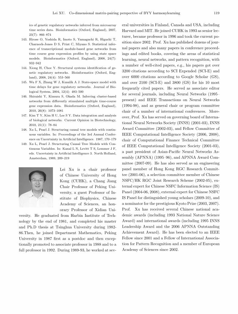
Lei XU. Co-dimensional matrix-pairing perspective of BYY harmonylearning 119
ics of genetic regulatory networks inferred from microarray
time series data. Bioinformatics (Oxford, England), 2007,
23(7): 866–874
143. Hirose O, Yoshida R, Imoto S, Yamaguchi R, Higuchi T,
Charnock-Jones D S, Print C, Miyano S. Statistical infer-
ence of transcriptional module-based gene networks from
time course gene expression profiles by using state space
models. Bioinformatics (Oxford, England), 2008, 24(7):
932–942
144. Xiong H, Choe Y. Structural systems identification of ge-
netic regulatory networks. Bioinformatics (Oxford, Eng-
land), 2008, 24(4): 553–560
145. Wu F X, Zhang W J, Kusalik A J. State-space model with
time delays for gene regulatory networks. Journal of Bio-
logical System, 2004, 12(4): 483–500
146. Shiraishi Y, Kimura S, Okada M. Inferring cluster-based
networks from differently stimulated multiple time-course
gene expression data. Bioinformatics (Oxford, England),
2010, 26(8): 1073–1081
147. Kim T Y, Kim H U, Lee S Y. Data integration and analysis
of biological networks. Current Opinion in Biotechnology,
2010, 21(1): 78–84
148. Xu L, Pearl J. Structuring causal tree models with contin-
uous variables. In: Proceedings of the 3rd Annual Confer-
ence on Uncertainty in Artificial Intelligence. 1987, 170–179
149. Xu L, Pearl J. Structuring Causal Tree Models with Con-
tinuous Variables. In: Kanal L N, Levitt T S, Lemmer J F,
eds. Uncertainty in Artificial Intelligence 3. North Holland,
Amsterdam, 1989, 209–219
Lei Xu is a chair professorof Chinese University of HongKong (CUHK), a Chang JiangChair Professor of Peking Uni-versity, a guest Professor of In-stitute of Biophysics, ChineseAcademy of Sciences, an hon-orary Professor of Xidian Uni-
versity. He graduated from Harbin Institute of Tech-nology by the end of 1981, and completed his masterand Ph.D thesis at Tsinghua University during 1982-86.Then, he joined Department Mathematics, PekingUniversity in 1987 first as a postdoc and then excep-tionally promoted to associate professor in 1988 and to afull professor in 1992. During 1989-93, he worked at sev-
eral universities in Finland, Canada and USA, includingHarvard and MIT. He joined CUHK in 1993 as senior lec-turer, became professor in 1996 and took the current po-sition since 2002. Prof. Xu has published dozens of jour-nal papers and also many papers in conference proceed-ings and edited books, covering the areas of statisticallearning, neural networks, and pattern recognition, witha number of well-cited papers, e.g., his papers got over3200 citations according to SCI Expended (SCI-E) andover 6000 citations according to Google Scholar (GS),and over 2100 (SCI-E) and 3800 (GS) for his 10 mostfrequently cited papers. He served as associate editorfor several journals, including Neural Networks (1995–present) and IEEE Transactions on Neural Networks(1994-98), and as general chair or program committeechair of a number of international conferences. More-over, Prof. Xu has served on governing board of Interna-tional Neural Networks Society (INNS) (2001-03), INNSAward Committee (2002-03), and Fellow Committee ofIEEE Computational Intelligence Society (2006, 2008),chair of Computational Finance Technical Committeeof IEEE Computational Intelligence Society (2001-03),a past president of Asian-Pacific Neural Networks As-sembly (APNNA) (1995–96), and APNNA Award Com-mittee (2007-09). He has also served as an engineeringpanel member of Hong Kong RGC Research Commit-tee (2001-06), a selection committee member of ChineseNSFC/HK RGC Joint Research Scheme (2002-05), ex-ternal expert for Chinese NSFC Information Science (IS)Panel (2004-06, 2008), external expert for Chinese NSFCIS Panel for distinguished young scholars (2009-10), anda nominator for the prestigious Kyoto Prize (2003, 2007).Prof. Xu has received several Chinese national aca-demic awards (including 1993 National Nature ScienceAward) and international awards (including 1995 INNSLeadership Award and the 2006 APNNA OutstandingAchievement Award). He has been elected to an IEEEFellow since 2001 and a Fellow of International Associa-tion for Pattern Recognition and a member of EuropeanAcademy of Sciences since 2002.