Life Estimation of Pressurized-Air Solar-Thermal John

David K. Fork1

e-mail: [email protected]

John Fitche-mail: [email protected]

Google, Inc.,

1600 Amphitheatre Pkwy,

Mountain View, CA 94043

Shawn ZiaeiIndependent Consultant


Robert I. JetterIndependent Consultant


Life Estimation ofPressurized-Air Solar-ThermalReceiver TubesThe operational conditions of the solar-thermal receiver for a Brayton cycle engine arechallenging, and lack a large body of operational data unlike steam plants. We explorethe receiver’s fundamental element, a pressurized tube in time varying solar flux for a se-ries of 30 yr service missions based on hypothetical power plant designs. We developedand compared two estimation methods to predict the receiver tube lifetime based onavailable creep life and fatigue data for alloy 617. We show that the choice of inelasticstrain model and the level of conservatism applied through design rules will vary the life-time predictions by orders of magnitude. Based on current data and methods, a turbineinlet temperature of 1120 K is a necessary 30-yr-life-design condition for our receiver.We also showed that even though the time at operating temperature is about three timeslonger for fossil fuel powered (steady) operation, the damage is always lower than cyclicoperation using solar power. [DOI: 10.1115/1.4007686]

Keywords: concentrating solar power, solar receiver, Brayton cycle, reliability, metalfatigue, creep, high temperature alloy, stress, strain

1 Introduction

For several decades researchers have considered using focusedsolar radiation to heat air in pressurized metal tubes to run Braytoncycle turbines [1–3]. The advantages include low water use; how-ever, from a materials standpoint, tubular air receivers are challeng-ing due to the combined effects of thermal oxidation, pressureinduced stress, diurnal thermal cycling, and thermal shocks fromcloud events; this paper looks at the latter three effects and exploresnecessary (though not sufficient) requirements.

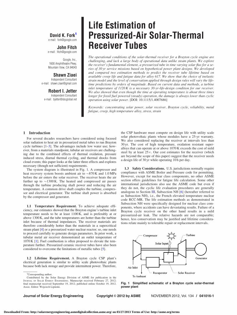
The system diagram is illustrated in Fig. 1. A compressor andheat recovery system boosts ambient air to �870 K and 1.0 MPabefore the air enters the solar receiver. The receiver heats the airfurther up to �1300 K. The heated and compressed air passesthrough the turbine producing shaft power and reducing the airtemperature. A common drive shaft couples the turbine, compres-sor and electrical generator. The turbine shaft power is absorbedby the compressor and generator.

1.1 Temperature Requirement. To achieve adequate effi-ciency, our estimates showed that the Brayton engine’s turbine inlettemperature needs to be at least 1100 K, and is preferably at orabove 1300 K, and the tube temperatures are hotter than the turbineinlet because of thermal impedances. The receiver materials aretherefore considerably hotter than the materials in a supercriticalsteam plant [4] or a pressurized water nuclear reactor; so, one needsto proceed carefully to generate design parameters. In prior work, atubular metal air receiver demonstrated an outlet temperature of1070 K [1]. Fuel combustion is often proposed to elevate the tem-perature further. Pressurized ceramic receiver tubes have also beenconsidered to overcome the limitations of metallic tubes [5].

1.2 Lifetime Requirement. A Brayton cycle CSP plant’selectrical generation is similar to utility scale photovoltaic plantsbecause both lack storage and provide intermittent power. Therefore,

the CSP hardware must compete on design life with utility scalesolar photovoltaic plants whose modules have a 25-yr warranty.We also considered replacing the receiver at intervals less than30 yr. The cost of high temperature, oxidation resistant super-alloys that can operate at or above 1070 K exceeds the cost of mildsteel by at least 25�. Our cost estimates for the receiver (whichare beyond the scope of this paper) suggest that the receiver needsa design life of 30 yr while operating 10 h per day.

1.3 Safety Considerations. U.S. jurisdictions normally requirecompliance with ASME Boiler and Pressure code for permitting.However, except for nuclear class components, no other ASMEsection offers guidelines for fatigue life calculation. Some otherinternational jurisdictions also use the ASME code but even ifthey do not, the cyclic life evaluation procedures are generallyanalogous to Section III, Subsection NH [6] (hereafter referred toas Subsection NH), i.e., the French elevated temperature nuclearcode RCC-MR. The life estimation methods as demonstrated inSubsection NH were specifically designed for nuclear class com-ponents, where accidents can have devastating results. Failure of aBrayton cycle receiver on the other hand results in a mildpressurized-air leak. The relative hazards are not comparable;hence, less conservatism may be justified and lifetime considera-tions relate mainly to tolerable repair or replacement intervals.

Fig. 1 Simplified schematic of a Brayton cycle solar-thermalpower plant

1Corresponding author.Contributed by the Solar Energy Division of ASME for publication in the

JOURNAL OF SOLAR ENERGY ENGINEERING. Manuscript received February 27, 2012;final manuscript received September 19, 2012; published online October 19, 2012.Assoc. Editor: Wojciech Lipinski.

Journal of Solar Energy Engineering NOVEMBER 2012, Vol. 134 / 041016-1Copyright VC 2012 by ASME

Downloaded From: http://solarenergyengineering.asmedigitalcollection.asme.org/ on 03/27/2013 Terms of Use: http://asme.org/terms

1.4 Cycling Loads. While base load power plants operate formonths under steady loads, peaker plants such as combined cycleplants are often operated several hours a day based on utilities’demand. These plants are designed for infrequent cold startups;daily “hot or warm” startups have smaller load amplitude com-pared to a cold start. In comparison, a solar-thermal receiver expe-riences daily cold startup with frequent warm startup/shutdowncycles during every cloud passage.

Heat transfer through the tube wall induces a temperature gradi-ent when the solar flux is present. Whereas some thermal stresses,such as cross-tube thermal gradients can be partially relieved bycarefully designed strain relief structures, cross-wall thermal gra-dients are necessary for heat transfer and are hence unavoidable;we consider the latter only in this study. It is also worth notingthat in real practice, heat exchangers often fail at the joints, a reli-ability topic not addressed here.

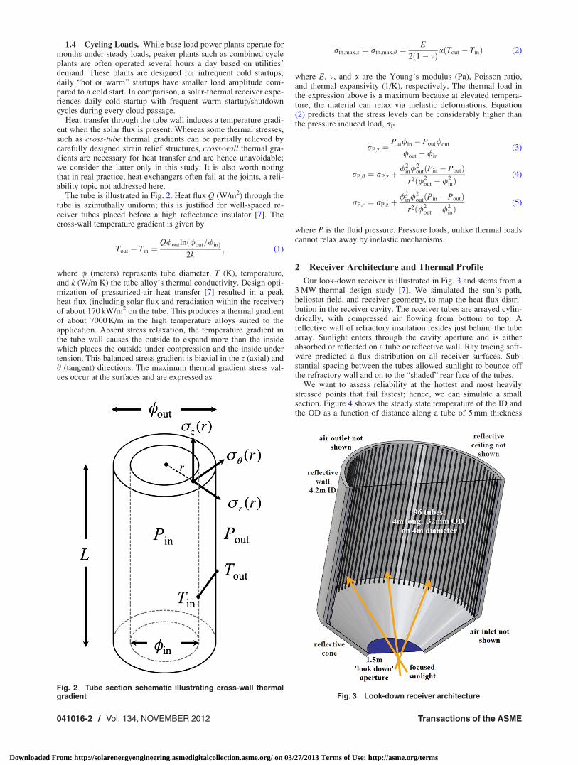
The tube is illustrated in Fig. 2. Heat flux Q (W/m2) through thetube is azimuthally uniform; this is justified for well-spaced re-ceiver tubes placed before a high reflectance insulator [7]. Thecross-wall temperature gradient is given by

Tout � Tin ¼Q/outlnð/out=/inÞ

2k; (1)

where / (meters) represents tube diameter, T (K), temperature,and k (W/m K) the tube alloy’s thermal conductivity. Design opti-mization of pressurized-air heat transfer [7] resulted in a peakheat flux (including solar flux and reradiation within the receiver)of about 170 kW/m2 on the tube. This produces a thermal gradientof about 7000 K/m in the high temperature alloys suited to theapplication. Absent stress relaxation, the temperature gradient inthe tube wall causes the outside to expand more than the insidewhich places the outside under compression and the inside undertension. This balanced stress gradient is biaxial in the z (axial) andh (tangent) directions. The maximum thermal gradient stress val-ues occur at the surfaces and are expressed as

rth;max;z ¼ rth;max;h ¼E

2ð1� vÞ aðTout � TinÞ (2)

where E, v, and a are the Young’s modulus (Pa), Poisson ratio,and thermal expansivity (1/K), respectively. The thermal load inthe expression above is a maximum because at elevated tempera-ture, the material can relax via inelastic deformations. Equation(2) predicts that the stress levels can be considerably higher thanthe pressure induced load, rP

rP;z ¼Pin/in � Pout/out

/out � /in

(3)

rP;h ¼ rP;z þ/2

in/2outðPin � PoutÞ

r2ð/2out � /2

inÞ(4)

rP;r ¼ rP;z þ/2

in/2outðPin � PoutÞ

r2ð/2out � /2

inÞ(5)

where P is the fluid pressure. Pressure loads, unlike thermal loadscannot relax away by inelastic mechanisms.

2 Receiver Architecture and Thermal Profile

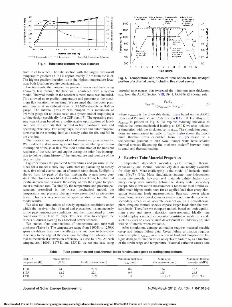
Our look-down receiver is illustrated in Fig. 3 and stems from a3 MW-thermal design study [7]. We simulated the sun’s path,heliostat field, and receiver geometry, to map the heat flux distri-bution in the receiver cavity. The receiver tubes are arrayed cylin-drically, with compressed air flowing from bottom to top. Areflective wall of refractory insulation resides just behind the tubearray. Sunlight enters through the cavity aperture and is eitherabsorbed or reflected on a tube or reflective wall. Ray tracing soft-ware predicted a flux distribution on all receiver surfaces. Sub-stantial spacing between the tubes allowed sunlight to bounce offthe refractory wall and on to the “shaded” rear face of the tubes.

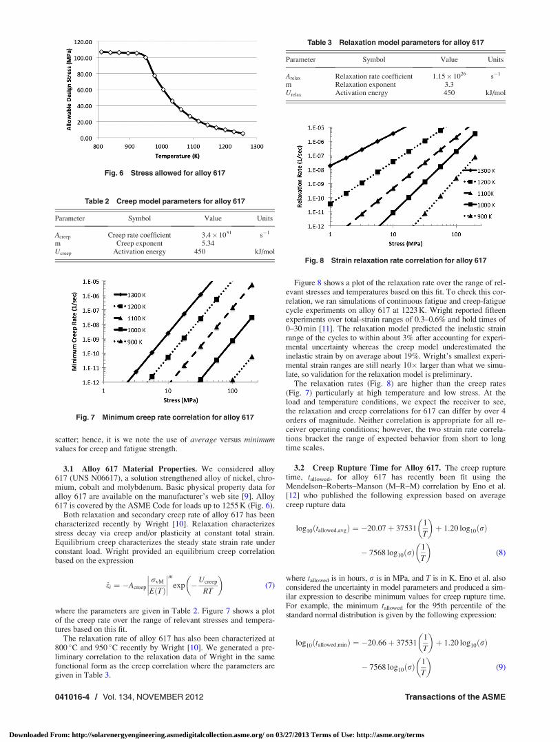
We want to assess reliability at the hottest and most heavilystressed points that fail fastest; hence, we can simulate a smallsection. Figure 4 shows the steady state temperature of the ID andthe OD as a function of distance along a tube of 5 mm thickness

Fig. 2 Tube section schematic illustrating cross-wall thermalgradient Fig. 3 Look-down receiver architecture

041016-2 / Vol. 134, NOVEMBER 2012 Transactions of the ASME


from inlet to outlet. The tube section with the largest cross-walltemperature gradient (31 K) is approximately 0.7 m from the inlet.The highest gradient location is not the highest temperature loca-tion; both locations require consideration.

For transients, the temperature gradient was scaled back usingFourier’s law through the tube wall, combined with a systemmodel. Thermal inertia in the receiver’s metal mass was included.This allowed us to predict temperature and pressure at the maxi-mum flux location, versus time. We assumed that the outer pres-sure remains at an ambient value of 0.1 MPa-absolute or 0 MPa-gauge. The internal pressure was ramped to a maximum of0.9 MPa-gauge for all cases based on a system model employing aturbine design specifically for a CSP plant [7]. The operating pres-sure was chosen based on a multivariable optimization of level-ized cost of electricity that factored in both hardware costs andoperating efficiency. For sunny days, the inner and outer tempera-tures rise in the morning, hold at a steady value for 6 h, and fall inthe evening.

The duration and coverage of cloud events vary considerably.We modeled a slow moving cloud front by simulating an 8-mininterruption of the solar flux. We used a simulation of the transientresponse of the receiver and engine during the solar flux interrup-tion to define a time history of the temperature and pressure of thereceiver tube.

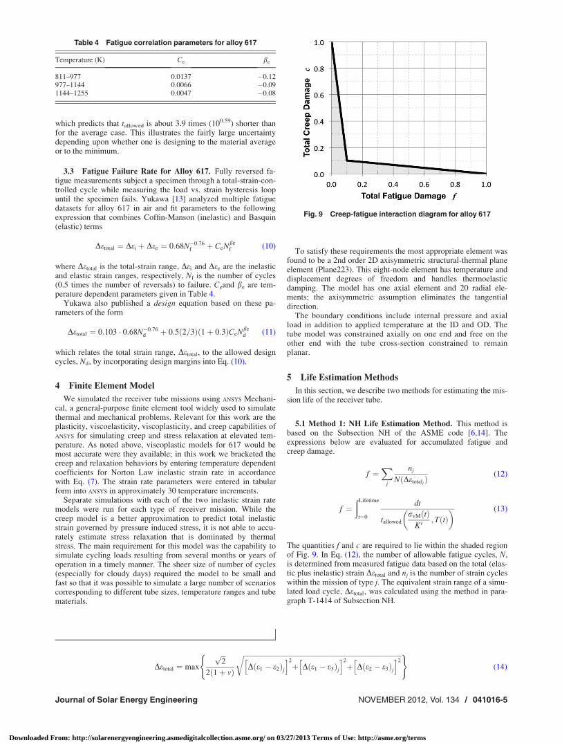
Figure 5 shows the predicted temperatures and pressure in thetubes for a model cloudy day, with start up plateauing to steadystate, five cloud events, and an afternoon ramp down. Sunlight isshaved from the peak of the day, making the system more con-stant. The cloud events block the sunlight for 8 min; but, thermalinertia and reradiation inside the cavity, allows the engine to oper-ate at a reduced rate. To simplify the temperature and pressure pa-rameters prescribed in the ANSYS mechanical model, thetemperature and pressure changes were prescribed as piecewiselinear. This is a very reasonable approximation of our thermalmodel results.

We also ran simulations of steady operation conditions underwhich the receiver tube is heated and pressurized instantaneouslyto the peak temperature conditions, and then maintained at thoseconditions for at least 90 days. This was done to compare theeffects of diurnal cycling to a baseload power scenario.

We studied four combinations of temperature and tube-wallthickness (Table 1). The temperature range from 1100 K to 1250 Kspans conditions from low-metallurgy risk and poor turbine-cycleefficiency to the edge of the code case for alloy 617 wherein ther-mal-to-mechanical conversion efficiency is close to 30%. At eachtemperature, 1100 K, 1175 K, and 1250 K, we ran one case using

imperial tube gauges that exceeded the minimum tube thickness,dmin from the ASME Section VIII, Div 1, UG-27(c)(1) design rule

dmin ¼Pin/in

2ðrallowed � 0:6PinÞ; (6)

where rallowed is the allowable design stress based on the ASMEBoiler and Pressure Vessel Code Section II Part D. For alloy 617,rallowed is plotted in Fig. 6. To explore reducing thickness toreduce the thermomechanical loading, at 1250 K we also includeda simulation with the thickness set to dmin. The simulation condi-tions are summarized in Table 1. Table 1 also shows the maxi-mum thermal stress calculated from Eq. (2) based on atemperature gradient of 7000 K/m; thinner walls have smallerthermal stresses illustrating the thickness tradeoff between hoopstrength and thermal loading.

3 Receiver Tube Material Properties

Temperature dependent modulus, yield strength, thermalexpansivity, and thermal conductivity data are readily availablefor alloy 617. More challenging is the model of inelastic strainrate _eiðr;TÞ (1/s). Most simulations assume time-independentstrain rate models; however, real materials exhibit higher (pri-mary) creep rates initially before the steady state (secondarycreep). Stress relaxation measurements (constant total strain) ex-hibit much higher strain rates for an applied load than creep elon-gation (constant load) measurements. Baseload power plantsspend long periods (weeks) under steady conditions during whichsecondary creep is an accurate description. In a solar-thermalplant, frequent thermal shocks impose larger loads than the pres-sure loads. Therefore we compare models based on both equilib-rium creep and stress relaxation measurements. Ideally, onewould employ a unified viscoplastic constitutive model in a codesuch as ANSYS or ABAQUS; such development is underway [8] andwill be of interest when available.

After simulation, damage estimation requires material specificcreep and fatigue failure data. Creep failure estimation requirestime-to-rupture, tallowed as a function of load and temperature. Fa-tigue damage estimation relies on cycles to failure Nf as a functionof the strain range and temperature. Material variation causes data

Fig. 4 Tube temperatures versus distance

Fig. 5 Temperature and pressure time series for the daylightportion of a diurnal cycle, including five cloud events

Table 1 Tube geometries and peak thermal loads for simulated peak operating temperatures

Peak IDtemperature (K)

Stress allowed(MPa) Inside diameter (mm)

Minimum thickness,dmin (mm)

Simulationthickness(es) (mm)

Maximum thermalstress(es) (MPa)

1100 24 29.3 0.6 1.24 19.51175 12.2 22.1 0.9 1.65 24.81250 5.5 19.9 1.8 1.8, 2.77 25.8, 39.7

Journal of Solar Energy Engineering NOVEMBER 2012, Vol. 134 / 041016-3


scatter; hence, it is we note the use of average versus minimumvalues for creep and fatigue strength.

3.1 Alloy 617 Material Properties. We considered alloy617 (UNS N06617), a solution strengthened alloy of nickel, chro-mium, cobalt and molybdenum. Basic physical property data foralloy 617 are available on the manufacturer’s web site [9]. Alloy617 is covered by the ASME Code for loads up to 1255 K (Fig. 6).

Both relaxation and secondary creep rate of alloy 617 has beencharacterized recently by Wright [10]. Relaxation characterizesstress decay via creep and/or plasticity at constant total strain.Equilibrium creep characterizes the steady state strain rate underconstant load. Wright provided an equilibrium creep correlationbased on the expression

_ei ¼ �Acreep

rvM

EðTÞ

��m

exp �Ucreep

RT

� �(7)

where the parameters are given in Table 2. Figure 7 shows a plotof the creep rate over the range of relevant stresses and tempera-tures based on this fit.

The relaxation rate of alloy 617 has also been characterized at800 �C and 950 �C recently by Wright [10]. We generated a pre-liminary correlation to the relaxation data of Wright in the samefunctional form as the creep correlation where the parameters aregiven in Table 3.

Figure 8 shows a plot of the relaxation rate over the range of rel-evant stresses and temperatures based on this fit. To check this cor-relation, we ran simulations of continuous fatigue and creep-fatiguecycle experiments on alloy 617 at 1223 K. Wright reported fifteenexperiments over total-strain ranges of 0.3–0.6% and hold times of0–30 min [11]. The relaxation model predicted the inelastic strainrange of the cycles to within about 3% after accounting for experi-mental uncertainty whereas the creep model underestimated theinelastic strain by on average about 19%. Wright’s smallest experi-mental strain ranges are still nearly 10� larger than what we simu-late, so validation for the relaxation model is preliminary.

The relaxation rates (Fig. 8) are higher than the creep rates(Fig. 7) particularly at high temperature and low stress. At theload and temperature conditions, we expect the receiver to see,the relaxation and creep correlations for 617 can differ by over 4orders of magnitude. Neither correlation is appropriate for all re-ceiver operating conditions; however, the two strain rate correla-tions bracket the range of expected behavior from short to longtime scales.

3.2 Creep Rupture Time for Alloy 617. The creep rupturetime, tallowed, for alloy 617 has recently been fit using theMendelson–Roberts–Manson (M–R–M) correlation by Eno et al.[12] who published the following expression based on averagecreep rupture data

log10ðtallowed;avgÞ ¼ �20:07þ 375311

T

� �þ 1:20 log10ðrÞ

� 7568 log10ðrÞ1

T

� �(8)

where tallowed is in hours, r is in MPa, and T is in K. Eno et al. alsoconsidered the uncertainty in model parameters and produced a sim-ilar expression to describe minimum values for creep rupture time.For example, the minimum tallowed for the 95th percentile of thestandard normal distribution is given by the following expression:

log10ðtallowed;minÞ ¼ �20:66þ 375311

T

� �þ 1:20 log10ðrÞ

� 7568 log10ðrÞ1

T

� �(9)

Fig. 6 Stress allowed for alloy 617

Table 2 Creep model parameters for alloy 617

Parameter Symbol Value Units

Acreep Creep rate coefficient 3.4� 1031 s�1

m Creep exponent 5.34Ucreep Activation energy 450 kJ/mol

Fig. 7 Minimum creep rate correlation for alloy 617

Table 3 Relaxation model parameters for alloy 617

Parameter Symbol Value Units

Arelax Relaxation rate coefficient 1.15� 1026 s�1

m Relaxation exponent 3.3Urelax Activation energy 450 kJ/mol

Fig. 8 Strain relaxation rate correlation for alloy 617



which predicts that tallowed is about 3.9 times (100.59) shorter thanfor the average case. This illustrates the fairly large uncertaintydepending upon whether one is designing to the material averageor to the minimum.

3.3 Fatigue Failure Rate for Alloy 617. Fully reversed fa-tigue measurements subject a specimen through a total-strain-con-trolled cycle while measuring the load vs. strain hysteresis loopuntil the specimen fails. Yukawa [13] analyzed multiple fatiguedatasets for alloy 617 in air and fit parameters to the followingexpression that combines Coffin-Manson (inelastic) and Basquin(elastic) terms

Detotal ¼ Dei þ Dee ¼ 0:68N�0:76f þ CeNbe

f (10)

where Detotal is the total-strain range, Dei and Dee are the inelasticand elastic strain ranges, respectively, Nf is the number of cycles(0.5 times the number of reversals) to failure. Ceand be are tem-perature dependent parameters given in Table 4.

Yukawa also published a design equation based on these pa-rameters of the form

Detotal ¼ 0:103 � 0:68N�0:76d þ 0:5ð2=3Þð1þ 0:3ÞCeNbe

d (11)

which relates the total strain range, Detotal, to the allowed designcycles, Nd, by incorporating design margins into Eq. (10).

4 Finite Element Model

We simulated the receiver tube missions using ANSYS Mechani-cal, a general-purpose finite element tool widely used to simulatethermal and mechanical problems. Relevant for this work are theplasticity, viscoelasticity, viscoplasticity, and creep capabilities ofANSYS for simulating creep and stress relaxation at elevated tem-perature. As noted above, viscoplastic models for 617 would bemost accurate were they available; in this work we bracketed thecreep and relaxation behaviors by entering temperature dependentcoefficients for Norton Law inelastic strain rate in accordancewith Eq. (7). The strain rate parameters were entered in tabularform into ANSYS in approximately 30 temperature increments.

Separate simulations with each of the two inelastic strain ratemodels were run for each type of receiver mission. While thecreep model is a better approximation to predict total inelasticstrain governed by pressure induced stress, it is not able to accu-rately estimate stress relaxation that is dominated by thermalstress. The main requirement for this model was the capability tosimulate cycling loads resulting from several months or years ofoperation in a timely manner. The sheer size of number of cycles(especially for cloudy days) required the model to be small andfast so that it was possible to simulate a large number of scenarioscorresponding to different tube sizes, temperature ranges and tubematerials.

To satisfy these requirements the most appropriate element wasfound to be a 2nd order 2D axisymmetric structural-thermal planeelement (Plane223). This eight-node element has temperature anddisplacement degrees of freedom and handles thermoelasticdamping. The model has one axial element and 20 radial ele-ments; the axisymmetric assumption eliminates the tangentialdirection.

The boundary conditions include internal pressure and axialload in addition to applied temperature at the ID and OD. Thetube model was constrained axially on one end and free on theother end with the tube cross-section constrained to remainplanar.

5 Life Estimation Methods

In this section, we describe two methods for estimating the mis-sion life of the receiver tube.

5.1 Method 1: NH Life Estimation Method. This method isbased on the Subsection NH of the ASME code [6,14]. Theexpressions below are evaluated for accumulated fatigue andcreep damage.

f ¼X

j

nj

NðDetotaljÞ(12)

f ¼ðLifetime

t¼0

dt

tallowed

rvMðtÞK0

; TðtÞ� � (13)

The quantities f and c are required to lie within the shaded regionof Fig. 9. In Eq. (12), the number of allowable fatigue cycles, N,is determined from measured fatigue data based on the total (elas-tic plus inelastic) strain Detotal and nj is the number of strain cycleswithin the mission of type j. The equivalent strain range of a simu-lated load cycle, Detotal, was calculated using the method in para-graph T-1414 of Subsection NH.

Detotal ¼ max

ffiffiffi2p

2ð1þ vÞ

ffiffiffiffiffiffiffiffiffiffiffiffiffiffiffiffiffiffiffiffiffiffiffiffiffiffiffiffiffiffiffiffiffiffiffiffiffiffiffiffiffiffiffiffiffiffiffiffiffiffiffiffiffiffiffiffiffiffiffiffiffiffiffiffiffiffiffiffiffiffiffiffiffiffiffiffiffiffiffiffiffiffiffiffiffiffiffiffiffiffiffiffiDðe1 � e2Þjh i2

þ Dðe1 � e3Þjh i2

þ Dðe2 � e3Þjh i2

r( )(14)

Table 4 Fatigue correlation parameters for alloy 617

Temperature (K) Ce be

811–977 0.0137 �0.12977–1144 0.0066 �0.091144–1255 0.0047 �0.08

Fig. 9 Creep-fatigue interaction diagram for alloy 617



where each of the following time series is calculated over one di-urnal cycle:

Dðe1 � e2Þj ¼ ðetotal;z � etotal;hÞj �max ðetotal;z � etotal;hÞjh i

(15)

Dðe1 � e3Þj ¼ ðetotal;z � etotal;rÞj �max ðetotal;z � etotal;rÞjh i

(16)

Dðe2 � e3Þj ¼ ðetotal;h � etotal;rÞj �max ðetotal;h � etotal;rÞjh i

(17)

and v, the Poisson ratio for elastic strain, is equal to 0.31.When choosing N in Eq. (12), as noted in Sec. 5.3, the nominal

Nf is less conservative than the design Nd. The fatigue measure-ments supporting this method don’t include a hold-time for creepbecause creep is accounted for in Eq. (13). In this expression,tallowed is the time to failure from creep rupture data at constantload and temperature. Subsection NH determines tallowed based onthe minimum strength, Eq. (9), and an equivalent stress thatadjusts the von Mises stress, rvM (from simulation) by a stresssafety factor, K0, where K0 ¼ 0.67. Subsection NH does not cur-rently cover alloy 617. K0 ¼ 0.67 for the alloys that SubsectionNH currently does cover. Air receiver failure is not especiallydangerous; hence, although not Subsection NH code-compliant,we also considered safety factor omission (K0 ¼ 1). The stress andtemperature vary throughout the mission, so the accumulatedcreep damage becomes an integral over the time series that wecomputed from the temperature and load data from ANSYS usingSimpson’s rule.

Figure 9 originates from design methods developed by Corumand Blass for alloy 617 in 1989 [15] and more recently corrobo-rated at Idaho National Laboratories [16]. Figure 9 accounts forthe interaction of fatigue damage f and creep damage c, which canbe significant for example when f¼ 0.1 due to the strong damagecompounding that occurs when both creep and fatigue are presentin appreciable amounts. Most of the data supporting the interac-tion diagram are for fatigue damage between 0.3 and 0.65.

As we will see, thermomechanical modeling of the solar re-ceiver predicts low fatigue damage, so more material characteriza-tion may be warranted for application of the Subsection NHmethod. When we adapt Eq. (12) for our solar-thermal receiver,the fatigue term sum becomes two terms corresponding to dailytotal strains and cloud event strains; however, as we will see, thefatigue terms we estimate for most receiver tube scenariosexplored are negligible.

5.2 Method 2: Life Estimation Based on MeasuredCreep-Fatigue Data. Carroll et al. [17] have measured the creep-fatigue interaction for high temperature nickel alloys, includingalloy 617 and Haynes 230. These measurements include creep-hold times of up to 30 min during the fatigue strain cycle; this isanalogous to the long periods of creep following diurnal or clouddriven thermal cycles. To exploit the similarity of measurementand operational conditions, we are proposing a life estimationmethod based on the inelastic strain amplitudes as follows:

FX

j

nj

NcfðDei;jÞ� 1:0 (18)

The design factor F is a value greater than 1, with higher valuesreflecting higher conservatism; F¼ 20 would be analogous withSubsection NH; however, there is no established operational basisfor this. Here, we propose that F¼ 10 is prudent for a solar appli-cation given that the CSP safety considerations are minor com-pared to the nuclear application for which NH was developed.Given our goal of designing a receiver that will survive 30 yr wemay reasonably expect that over the distribution of tubes in the re-ceiver, some will fail at Ncf/10 cycles. Ncf is the creep-fatigue lifedetermined from the inelastic strain amplitude Dei;j of the jth type(daily cycles or cloud event types). Although it is not generally

true for all high temperature alloys, for the nickel based superal-loys 617 and Haynes 230, we have noted that between about1073 K and 1200 K, inelastic strain predicts creep-fatigue lifeaccording to the Coffin Manson correlation

Dei ¼ CiNbicf (19)

particularly for small strain amplitudes like those in the solar-thermal receiver. As a check, we compared the predictions of cor-relations based on the data of Carroll et al. [17], Lu et al. [18], andmore recent data [19]. At low strain amplitude the agreementbetween low cycle fatigue data and creep-fatigue data are close;all of the correlations that we compared agreed to within a factorof two for strain ranges smaller than 0.1%. For this study, we usethe correlation published by Lu et al. in which Ci¼ 1.39, andbi ¼ �0:8828. We note with some caution that higher tempera-ture data collected by Carroll et al. show that at 1273 K the fatiguedamage occurs more rapidly with cycling. Therefore, for tempera-tures above 1200 K, one might use a temperature dependentCoffin-Manson relationship and recognize that method 2 repre-sents a necessary but not sufficient reliability condition. If thestrain cycles can be generalized to either daily strain events orcloud events, then Eq. (18) reduces to

10ndays

NcfðDei=dayÞþ nclouds

NcfðDei=cloudÞ

� �� 1:0 (20)

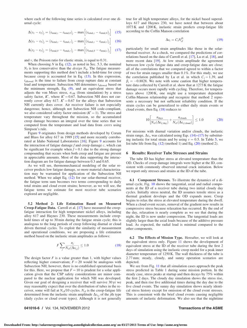
For missions with diurnal variation and/or clouds, the inelasticstrain range, Dei, was calculated using Eqs. (14)–(17) by substitut-ing inelastic for total strain and by using v ¼ 0:5. In Table 5, welist tube life from Eq. (12) (method 1) and Eq. (20) (method 2).

6 Results: Receiver Tube Stresses and Strains

The tube ID has higher stress at elevated temperature than theOD. Checks of creep damage integrals were higher at the ID, con-sistent with commonly observed internal crack initiation. Belowwe report only stresses and strains at the ID of the tube.

6.1 Component Stresses. To illustrate the dynamics of a di-urnal cycle, Fig. 10 shows the tangential, axial and radial compo-nents at the ID of a receiver tube during two initial cloudy daycycles. Initially stress neutral, the ID assumes tensile stress as athermal gradient develops and the OD expands more. Creepbegins to relax the stress at elevated temperature during the dwell.When a cloud event occurs, removal of the gradient now results incompressive stress because relaxation has occurred. By the end ofthe day, relaxation is nearly complete as we see that during thenight, the ID is now under compression. The tangential loads areslightly larger than the axial loads because of the additive pressureload. As expected, the radial load is minimal compared to theother components.

6.2 The Effects of Mission Type. Hereafter, we will look atthe equivalent stress only. Figure 11 shows the development ofequivalent stress at the ID of the receiver tube during the first 2days of simulation using the inelastic creep model for a peak innerdiameter temperature of 1250 K. The wall thickness of the tube is2.77 mm; steady, cloudy, and sunny operation scenarios aredepicted.

We see from Fig. 11 that all simulation cases approach the peakstress predicted in Table 1 during some mission portion. In thesteady case, stress peaks at startup and then decays by 75% withinthe first 2 days. The cloudy day simulation shows the stress rise,peak, and then rise five additional times during the day due to thefive cloud events. The sunny day simulation shows nearly identi-cal stress history except for omission of the cloud event stresses.This is consistent with the brief cloud events causing negligibleamounts of inelastic deformation. We also see that the nighttime



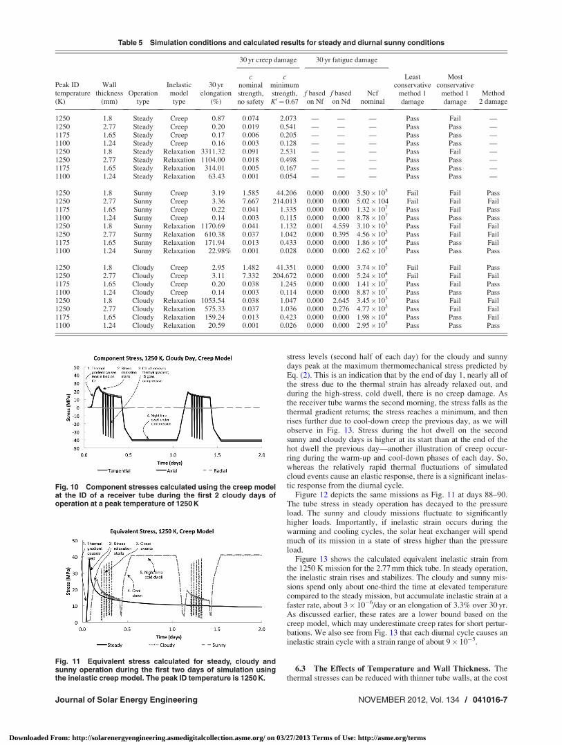
stress levels (second half of each day) for the cloudy and sunnydays peak at the maximum thermomechanical stress predicted byEq. (2). This is an indication that by the end of day 1, nearly all ofthe stress due to the thermal strain has already relaxed out, andduring the high-stress, cold dwell, there is no creep damage. Asthe receiver tube warms the second morning, the stress falls as thethermal gradient returns; the stress reaches a minimum, and thenrises further due to cool-down creep the previous day, as we willobserve in Fig. 13. Stress during the hot dwell on the secondsunny and cloudy days is higher at its start than at the end of thehot dwell the previous day—another illustration of creep occur-ring during the warm-up and cool-down phases of each day. So,whereas the relatively rapid thermal fluctuations of simulatedcloud events cause an elastic response, there is a significant inelas-tic response from the diurnal cycle.

Figure 12 depicts the same missions as Fig. 11 at days 88–90.The tube stress in steady operation has decayed to the pressureload. The sunny and cloudy missions fluctuate to significantlyhigher loads. Importantly, if inelastic strain occurs during thewarming and cooling cycles, the solar heat exchanger will spendmuch of its mission in a state of stress higher than the pressureload.

Figure 13 shows the calculated equivalent inelastic strain fromthe 1250 K mission for the 2.77 mm thick tube. In steady operation,the inelastic strain rises and stabilizes. The cloudy and sunny mis-sions spend only about one-third the time at elevated temperaturecompared to the steady mission, but accumulate inelastic strain at afaster rate, about 3� 10�6/day or an elongation of 3.3% over 30 yr.As discussed earlier, these rates are a lower bound based on thecreep model, which may underestimate creep rates for short pertur-bations. We also see from Fig. 13 that each diurnal cycle causes aninelastic strain cycle with a strain range of about 9� 10�5.

6.3 The Effects of Temperature and Wall Thickness. Thethermal stresses can be reduced with thinner tube walls, at the cost

Table 5 Simulation conditions and calculated results for steady and diurnal sunny conditions

30 yr creep damage 30 yr fatigue damage

Peak IDtemperature(K)

Wallthickness

(mm)Operation

type

Inelasticmodeltype

30 yrelongation

(%)

cnominalstrength,no safety

cminimumstrength,K0 ¼ 0.67

f basedon Nf

f basedon Nd

Ncfnominal

Leastconservative

method 1damage

Mostconservative

method 1damage

Method2 damage

1250 1.8 Steady Creep 0.87 0.074 2.073 — — — Pass Fail —1250 2.77 Steady Creep 0.20 0.019 0.541 — — — Pass Pass —1175 1.65 Steady Creep 0.17 0.006 0.205 — — — Pass Pass —1100 1.24 Steady Creep 0.16 0.003 0.128 — — — Pass Pass —1250 1.8 Steady Relaxation 3311.32 0.091 2.531 — — — Pass Fail —1250 2.77 Steady Relaxation 1104.00 0.018 0.498 — — — Pass Pass —1175 1.65 Steady Relaxation 314.01 0.005 0.167 — — — Pass Pass —1100 1.24 Steady Relaxation 63.43 0.001 0.054 — — — Pass Pass —

1250 1.8 Sunny Creep 3.19 1.585 44.206 0.000 0.000 3.50� 105 Fail Fail Pass1250 2.77 Sunny Creep 3.36 7.667 214.013 0.000 0.000 5.02� 104 Fail Fail Fail1175 1.65 Sunny Creep 0.22 0.041 1.335 0.000 0.000 1.32� 107 Pass Fail Pass1100 1.24 Sunny Creep 0.14 0.003 0.115 0.000 0.000 8.78� 107 Pass Pass Pass1250 1.8 Sunny Relaxation 1170.69 0.041 1.132 0.001 4.559 3.10� 103 Pass Fail Fail1250 2.77 Sunny Relaxation 610.38 0.037 1.042 0.000 0.395 4.56� 103 Pass Fail Fail1175 1.65 Sunny Relaxation 171.94 0.013 0.433 0.000 0.000 1.86� 104 Pass Pass Fail1100 1.24 Sunny Relaxation 22.98% 0.001 0.028 0.000 0.000 2.62� 105 Pass Pass Pass

1250 1.8 Cloudy Creep 2.95 1.482 41.351 0.000 0.000 3.74� 105 Fail Fail Pass1250 2.77 Cloudy Creep 3.11 7.332 204.672 0.000 0.000 5.24� 104 Fail Fail Fail1175 1.65 Cloudy Creep 0.20 0.038 1.245 0.000 0.000 1.41� 107 Pass Fail Pass1100 1.24 Cloudy Creep 0.14 0.003 0.114 0.000 0.000 8.87� 107 Pass Pass Pass1250 1.8 Cloudy Relaxation 1053.54 0.038 1.047 0.000 2.645 3.45� 103 Pass Fail Fail1250 2.77 Cloudy Relaxation 575.33 0.037 1.036 0.000 0.276 4.77� 103 Pass Fail Fail1175 1.65 Cloudy Relaxation 159.24 0.013 0.423 0.000 0.000 1.98� 104 Pass Pass Fail1100 1.24 Cloudy Relaxation 20.59 0.001 0.026 0.000 0.000 2.95� 105 Pass Pass Pass

Fig. 10 Component stresses calculated using the creep modelat the ID of a receiver tube during the first 2 cloudy days ofoperation at a peak temperature of 1250 K

Fig. 11 Equivalent stress calculated for steady, cloudy andsunny operation during the first two days of simulation usingthe inelastic creep model. The peak ID temperature is 1250 K.



of increased pressure loads. Reduced temperature also reducesinelastic strain rates for a given load.

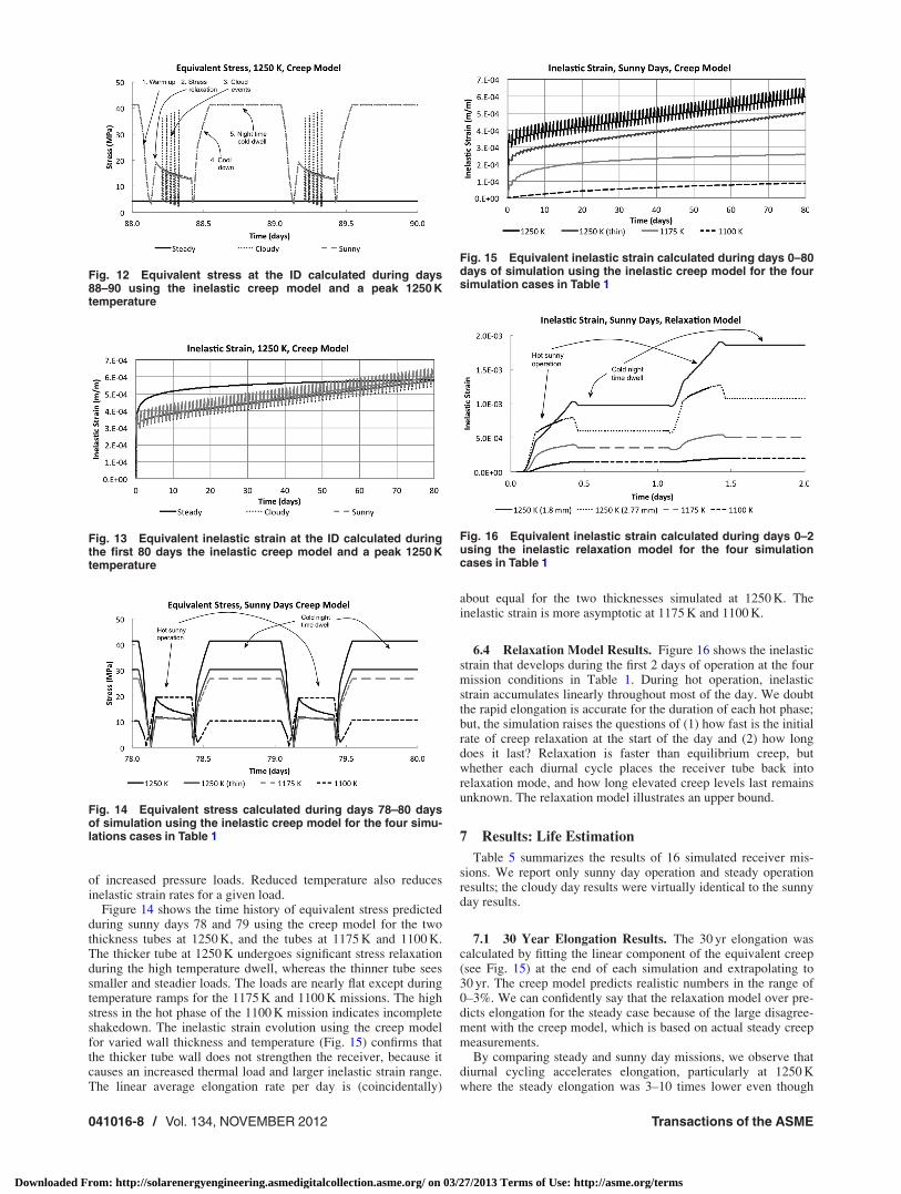
Figure 14 shows the time history of equivalent stress predictedduring sunny days 78 and 79 using the creep model for the twothickness tubes at 1250 K, and the tubes at 1175 K and 1100 K.The thicker tube at 1250 K undergoes significant stress relaxationduring the high temperature dwell, whereas the thinner tube seessmaller and steadier loads. The loads are nearly flat except duringtemperature ramps for the 1175 K and 1100 K missions. The highstress in the hot phase of the 1100 K mission indicates incompleteshakedown. The inelastic strain evolution using the creep modelfor varied wall thickness and temperature (Fig. 15) confirms thatthe thicker tube wall does not strengthen the receiver, because itcauses an increased thermal load and larger inelastic strain range.The linear average elongation rate per day is (coincidentally)

about equal for the two thicknesses simulated at 1250 K. Theinelastic strain is more asymptotic at 1175 K and 1100 K.

6.4 Relaxation Model Results. Figure 16 shows the inelasticstrain that develops during the first 2 days of operation at the fourmission conditions in Table 1. During hot operation, inelasticstrain accumulates linearly throughout most of the day. We doubtthe rapid elongation is accurate for the duration of each hot phase;but, the simulation raises the questions of (1) how fast is the initialrate of creep relaxation at the start of the day and (2) how longdoes it last? Relaxation is faster than equilibrium creep, butwhether each diurnal cycle places the receiver tube back intorelaxation mode, and how long elevated creep levels last remainsunknown. The relaxation model illustrates an upper bound.

7 Results: Life Estimation

Table 5 summarizes the results of 16 simulated receiver mis-sions. We report only sunny day operation and steady operationresults; the cloudy day results were virtually identical to the sunnyday results.

7.1 30 Year Elongation Results. The 30 yr elongation wascalculated by fitting the linear component of the equivalent creep(see Fig. 15) at the end of each simulation and extrapolating to30 yr. The creep model predicts realistic numbers in the range of0–3%. We can confidently say that the relaxation model over pre-dicts elongation for the steady case because of the large disagree-ment with the creep model, which is based on actual steady creepmeasurements.

By comparing steady and sunny day missions, we observe thatdiurnal cycling accelerates elongation, particularly at 1250 Kwhere the steady elongation was 3–10 times lower even though

Fig. 12 Equivalent stress at the ID calculated during days88–90 using the inelastic creep model and a peak 1250 Ktemperature

Fig. 14 Equivalent stress calculated during days 78–80 daysof simulation using the inelastic creep model for the four simu-lations cases in Table 1

Fig. 15 Equivalent inelastic strain calculated during days 0–80days of simulation using the inelastic creep model for the foursimulation cases in Table 1

Fig. 16 Equivalent inelastic strain calculated during days 0–2using the inelastic relaxation model for the four simulationcases in Table 1

Fig. 13 Equivalent inelastic strain at the ID calculated duringthe first 80 days the inelastic creep model and a peak 1250 Ktemperature



the hot dwell was more than 2.5 times longer. This is somewhatexpected because the elongation is driven by a creep process thatscales as the sum of pressure and thermal stresses raised to thefifth power; higher average loads increase elongation super-linearly.

7.2 Method 1 Damage. To estimate the 30 yr creep damagereported in Table 5, we ran the simulation to the point of stabiliza-tion, typically 90–360 days, and then integrated the creep damagein expression (Eq. (13)) for the last 7 days and then multiplied by52� 30. For the steady operation case, this represents 262,080 hof hot operation, whereas for the sunny day simulation, the re-ceiver is hot for 109,200 h over 30 yr. As discussed above, whencalculating the creep damage, there is a choice of nominal vs.minimum creep strength and whether to apply a safety factor. Ta-ble 5 reports the 30 yr creep damage integral for the two endcases: nominal creep strength with no safety factor and minimumcreep strength with a safety factor of 0.67.

We calculated cycles to failure from the total equivalent strainrange, Detotal. The fatigue damage portion, f, of method 1, Eq.(12), was negligible for all cases calculated with the creep modelbecause of the small total-strain range which, according to Eq.(14), has Nd> 106 cycles. There are no cyclic loads for the steadycase, so strain ranges and cycles-to-failure calculations are omit-ted in Table 5. Table 5 reports 30-yr fatigue damage f for both thenominal Nf (Eq. (10)) and the design Nd (Eq. (11)) cycles to fail-ure for sunny days.

The predictions of method 1 are highly dependent on one’schoices of nominal vs. minimum strength, the safety factor, andwhether one uses the nominal or design cycles to failure. Somejurisdictions will require the most conservative combination. InTable 5, we report the least and most conservative combinationsof these choices, using 10,920 for ndays.

We see that all of the steady operation cases meet the method 1design criteria (c and f within the shaded portion of Fig. 9) withthe exception of the thin (1.8 mm) tube at 1250 K for the mostconservative criteria. The latter occurs because the thickness isbased on Section VIII allowable stress levels and the creep dam-age criteria in Subsection NH are more conservative than those inSection VIII. The results are largely independent of whether thecreep or relaxation model is used because for both models, thetube stresses relax to the pressure loads at long times.

We also see that for sunny (and cloudy) operation the damageestimates are highly dependent on the model choice and the levelof conservatism. The creep model predicts higher stress levels andhence more creep damage. The relaxation model predicts higherstrain ranges and hence more fatigue damage. Depending on one’slevel of conservatism, the damage estimates c and f can differ byseveral orders, and an additional factor of 10 or more dependingon the inelastic strain model. Clearly, a narrowing of these optionsthrough better models, and a data-based set of life estimation rulesis needed. Unfortunately, laboratory, or plant operation data forthe combination of high temperature, low cycle amplitude, andlarge cycle number is not available.

What we can conclude from the range of method 1 damage cal-culations is that the 1250 K operating point appears risky exceptfor steady operation; the creep model predicts failure, particularlyfor the thick walled tube. A viscoplastic model might predicthigher life estimates if stresses relax quickly at short times andstrain rates slow to secondary rates thereafter. The 1175 K opera-tion case is marginal based on the creep damage model because itfails the most conservative strength and safety factor combination.There is a generous design space at 1100 K, and a possibility todesign at higher pressure.

7.3 Method 2 Creep-Fatigue Damage Results. As withmethod 1, sunny and cloudy days exhibit very similar damage.Table 5 only lists results for sunny days and the failure criterioneffectively reduced to 10ndays=Ncf < 1. The strain ranges were

highly dependent on whether we used the creep or relaxationinelastic strain model, the creep model being less conservative.The creep model suggests that only the thick walled tube at1250 K would fail, and the relaxation model suggests that only thetube at 1100 K would survive. Given that the creep and relaxationmodels bracket the expected behavior of the inelastic strain, weexpect that the actual design space lies somewhere in between thetwo cases. This is consistent with the life estimation results ofmethod 1.

8 Discussion

8.1 The Pressurized-Air Brayton CSP Presents ParticularChallenges. What makes air an attractive heat transfer fluid is theinexhaustible supply surrounding the power plant that obviatingthe need for expensive cooling and recirculation. However, air isalso a poor heat transfer fluid; design considerations [7] limitedthe solar flux for the pressurized-air design to only 170 kW/m2

compared to about 1000 kW/m2 for some lower temperature, lowpressure molten salt designs. In spite of the low flux, we could notpredictably meet design objectives at the highest temperatures tar-geted. Compared to commercial CSP steam plants that operate atup to about 950 K, design for air in the 1100 K–1250 K rangerequires a detailed understanding of creep and much larger re-ceiver area per unit of thermal power.

8.2 Need for Better Inelastic Models. We saw >10� pre-dicted lifetime variation between the creep and relaxation models;but, we also expect both models capture relevant long and short-term responses to pressure and thermal loads, respectively. A gen-eral viscoplastic model [8] for the high temperature alloys ofchoice is needed and, when available, could narrow the range ofdamage predictions reported here. A viscoplastic model mightpredict a larger design space than we have seen. Much depends onhow fast the response is to perturbations on the scale of thermalevents.

8.3 Inelastic Damage Accrues Slowly. There was little dif-ference between cloudy and sunny missions; brief thermal eventslike the fast passage of a small cloud bank, produced large stressresponses but little creep. The most damaging thermal cycleswere the diurnal cycles that occurred slowly enough for creep tooccur. Although it may not be practical, this suggests that (1) amore binary application of radiation (full or none) to the receivermay have certain advantages at high temperatures and (2) moregradual cloud events than those considered here may be moredamaging and may need further consideration.

8.4 Need for Better, Data-Based, Lifetime Estimates. Weshowed that lifetime estimates depend more than an order of mag-nitude on how far one relaxes conservative design rule choicesbased on minimum material strength and safety factors. It willtake operating data or lengthy laboratory experiments under com-parable conditions to establish appropriate design rules; currently,the creep rupture data are based on a load history unlike our appli-cation, and the fatigue data are based on strain rates and ampli-tudes unlike the receiver mission. The fatigue data we base ourcalculations on are isothermal; however, thermofatigue cyclingcan be up to 10� more damaging [20] and is also time consumingto characterize.

The conventional way (method 1) of calculating fatigue damagefrom total strain predicts negligible fatigue, whereas method 2based on the inelastic strain, does predict damage. It may be bene-ficial to avoid lifetime estimates based on summing separate creepand fatigue contributions, both of which are based on measure-ment conditions that differ greatly from the operational mission.Method 2 has the shortcoming that it does not address noncyclicdamage. Incorporation of a second criterion, such as a total elon-gation limit might address this shortcoming.



8.5 The Highest Temperature Operating ConditionAppears Difficult. This study casts doubt that 1250 K is a suita-ble design temperature for the receiver, which is somewhat disap-pointing because the turbine can be designed for still much highertemperature and efficiency. Thin walled tubes have lower missiondamage estimates; however, especially at the highest tempera-tures, thin walled tubes may be susceptible to corrosion failure ifthe chromium can evaporate. At high temperatures diurnal cyclingaccelerates elongation. 1175 K may be a suitable tube ID tempera-ture, which would result in a turbine inlet temperature of about850 �C, not unlike past designs [1]. The design space can be morethoroughly explored; but it is prudent first to prepare better mod-els and design criteria and to carefully examine the overall planteconomics.

8.6 Steady Operation is Always Less Damaging. We seefrom Figs. 11 and 12 that the loads and cumulative inelasticstrains are always lower for steady operation (after an initial burn-in phase). Table 5 confirms that cumulative damage is lower, evenwhen the hot-service time is about 3 times longer. This shows thatdiurnal variation will make any Brayton cycle plant with a heatexchanger less reliable than baseload operation. A corollary tothis is further improvements in Brayton cycle CSP plants mayalso make electricity from fossil energy such as coal more dis-patchable, thereby increasing coal plant profitability by allowingmore frequent ramping.

9 Conclusions

It is challenging to design a pressurized-air solar-thermal re-ceiver for a Brayton cycle engine due to difficulties relating tofinding adequate materials and modeling their properties. In par-ticular, here are five key challenges:

• Time dependent creep phenomena are significant in the ele-vated temperature and cycle regime. Model results show thatthe speed and extent to which creep behaviors cycle betweenprimary and secondary rates will have a strong influence onmechanical damage.

• The models needed to describe this creep behavior areunderdeveloped.

• The data needed to produce predictive time dependent creepmodels are incomplete and is understandably difficult togather because of the high temperatures and high measure-ment precision required for small amplitude strains.

• The extent to which conservative design parameters can besafely relaxed is not known and the sensitivity of lifetimeestimates to such parameters is large: �10� changes from50% changes in safety factor for example.

• Thickness allowances for corrosion and thermomechanicalfatigue effects complicate the damage assessment becauselifetime estimates are highly thickness dependent.

Pressurized-air Brayton CSP plants remain an interesting con-cept; however, the issues raised herein must be more fully exam-ined and resolved before costs and service life estimates can becalculated with the accuracy needed for project evaluation. Basedon current data and methods, a turbine inlet temperature of1120 K is a necessary upper limit for tube reliability in our CSPdesign and 1050 K is a sufficient upper limit. CSP plants requireconsiderable cost reductions from their current status in order tocompete directly with fossil energy without subsidy. Furthermore,making heat exchangers more cycle-able for use in solar applica-tions will also increase the cycle-ability of coal powered electric-ity thereby making the latter cheaper and more attractive.

Acknowledgment

This paper is dedicated in memory of Timothy Allen. Weacknowledge useful discussions with Kevin Chen and RossKoningstein of Google, Philip Gleckman (now at Areva), Alec

Brooks (now at AeroVironment), Darrell Socie of eFatigue, LauraCarroll, and Jill Wright of Idaho National Laboratory, Sam Shamof ORNL, Andy Jones and Gordon Tatlock of U. of Liverpool,David Metzler of Haynes Intl. and Fred Starr.

Nomenclature

A ¼ creep rate coefficient, s�1

C ¼ fatigue coefficientc ¼ creep damage integrald ¼ tube-wall thickness, mE ¼ Young’s modulus, PaF ¼ method 2 damage factorf ¼ fatigue damage sum

K0 ¼ inelastic stress safety factork ¼ thermal conductivity, W/m KN ¼ allowable cycles to failurem ¼ Norton creep rate exponentn ¼ applied cyclesP ¼ pressure, PaQ ¼ heat flux, W/m2

R ¼ noble gas constant, J/mol Kr ¼ radial position, mT ¼ temperature, Kt ¼ time, S

U ¼ activation energy, J

Greek Letters

a ¼ thermal expansivity, m/m Kb ¼ fatigue exponent/ ¼ diameter, me ¼ strain, m/mt ¼ Poisson ratior ¼ stress, Pa

Subscripts

allowed ¼ allowance from lifetime measurement dataavg ¼ average

cf ¼ creep-fatigue cyclesclouds ¼ clouds during receiver design life/cloud ¼ per cloud event cyclecreep ¼ creep mechanismdays ¼ days during receiver design life/day ¼ per diurnal cycle

d ¼ design cyclese ¼ elasticf ¼ fatigue cyclesi ¼ inelastic

in ¼ inner, insidej ¼ time series subscript

max ¼ maximummin ¼ minimumout ¼ outer, outside

P ¼ pressurer ¼ radial

relaxation ¼ relaxation mechanismt ¼ transients

th ¼ thermaltotal ¼ inelastic plus elasticvM ¼ von Mises

z ¼ axialh ¼ tangential

Acronyms

CSP ¼ concentrating solar powerID ¼ inner diameter

OD ¼ outer diameter



References

[1] Amsbeck, L., Denk, T., Ebert, M. Gertig, C., Heller, P., Herrmann, P., Jedam-ski, J., John J., Pitz-Paal, R., Prosinecki, T., Rehn, J., Reinalter, W., and Uhlig,R., 2010, “Test of a Solar-Hybrid Microturbine System and Evaluation of Stor-age Deployment,” Proceedings of SolarPaces, Pirpignan, France, September21–24, Paper No. 0177.

[2] Stein, W., Kim, J.-S., Burton, A., McNaughton, R., Soo Too, Y. C., McGregor,J., Nakatani, H., Tagawa, M., Osada, T., Okubo, T., Kobayashi, K., 2010,“Design and Construction of a 200 kWe Tower Brayton Cycle Power Plant,”Proceedings of SolarPaces, Pirpignan, France, September 21–24, Paper No.0289.

[3] 2012, “RE<C: Brayton Project Overview,” Google.org, Mountain View, CA,http://www.google.org/pdfs/google_brayton_summary.pdf

[4] Phillips, J., and Shingledecker, J., 2011, “U.S. Department of Energy and OhioCoal Development Office Advanced Ultra-Supercritical Materials Project forBoilers and Steam Turbines, Summary of Results,”Electric Power ResearchInstitute, Palo Alto, CA, Report No. 1022770.

[5] Smith, K. O., 1984, “Ceramic Heat Exchanger Design Methodology,” ArgonneNational Laboratory, Argonne, Report No. ANL/FE-84-6.

[6] ASME, “2010 ASME Boiler & Pressure Vessel Code, Section III, SubsectionNH, Class 1 Components in Elevated Temperature Service,” The American So-ciety of Mechanical Engineers, Fairfield, NJ.

[7] Google, 2012 “Brayton System Hardware Summary,” Google.org, MountainView, http://www.google.org/pdfs/google_brayton_system_hardware.pdf

[8] Sham, T.-L., and Walker, K. P., 2008, “Preliminary Development of a UnifiedViscoplastic Constitutive Model for Alloy 617 With Special Reference to LongTerm Creep Behavior,” Proceedings of 4th International Topical Meeting onHigh Temperature Reactor Technology (HTR2008), Washington, DC, Septem-ber 28–October 1, Vol. 2, Paper No. HTR2008-85215, pp. 81–89.

[9] Special Metals Corporation, 2005 “InconelVR

Alloy 617,” Publication NumberSMC-029, http://www.specialmetals.com/documents/Inconel%20alloy%20617.pdf

[10] Wright, J. K., 2011, “Strain Rate Sensitivity of Alloy 617,” Very High Temper-ature Reactor (VHTR) R&D 4th Annual Technical Review Meeting, Albuquer-que, NM, Presentation 08 Wright J—Stress.

[11] Wright, J. K., Carroll, L. J., Cabet, C., Lillo, T. M., Benz, J. K., Simpson, J. A.,Lloyd, W. R., Chapman, J. A., and Wright, R.N., 2011, “Characterization ofElevated Temperature Properties of Heat Exchanger and Steam GeneratorAlloys,” Nucl. Eng. Des., 251, pp. 252–260.

[12] Eno, D. R., Young, G. A., and Sham, T.-L., 2008, “A Unified View ofEngineering Creep Parameters,” Proceedings of ASME Pressure Vessels andPiping Division Conference (PVP2008), Chicago, July 27–31, ASME PaperNo. 61129, pp. 777–792.

[13] Yukawa, S., 1991, “Elevated Temperature Fatigue Design Curves for Ni-Cr-Co-Mo Alloy 617,” The 1st JSME/ASME Joint International Conference onNuclear Engineering, Tokyo, November 4–7, pp. 1–6.

[14] Dhalla, A. K., 1991, “Recommended Practices in Elevated TemperatureDesign: A Compendium of Breeder Reactor Experience. (1970–1987) VolumeI—Current Status and Future Directions,” Bulletin 362, Welding ResearchCouncil, New York.

[15] Corum, J. M., and Blass, J. J., 1991, “Rules for Design of Alloy 617 NuclearComponents to Very High Temperatures,” ASME Pressure Vessel Piping, 215,pp. 147–153.

[16] Wright, J., and Sham, S., 2010, “Creep-Fatigue Interaction Diagram for Alloy617 in Air at 950 �C,” Engineering Calculations and Analysis Report 1199,Idaho National Laboratory, Idaho Falls, ID.

[17] Carroll, L. J., Lloyd, W. R., Simpson, J. A., and Wright, R. N., 2011, “TheInfluence of Dynamic Strain Aging on Fatigue and Creep-Fatigue Characteriza-tion of Nickel-Base Solid Solution Strengthened Alloys,” Mater. High Temp.,27(4), pp. 313–323.

[18] Lu, Y. L., Chen, L. J., Wang, G. Y., Benson, M. L., Liaw, P. K., Thompson, S.A., Blust, J. W., Browning, P. F., Bhattacharya, A. K., Aurrecoechea, J. M., andKlarstrom D. K., 2005, “Hold-Time Effects on Low-Cycle Fatigue Behaviorof Haynes 230 Superalloy at High Temperatures,” Mater. Sci. Eng.: A, 409,pp. 282–291.

[19] Carroll, L. J., Carroll, M. C., Cabet, C., and Wright, R.N., “The Developmentand Impact of Microstructural Damage During High Temperature Creep-Fatigue of a Nickel-Base Austenitic Alloy,” Int. J. Fatigue (accepted).

[20] Jaske, C. E., 1976, “Thermal Fatigue of Materials and Components,” ReportNo. ASTM STP 612, pp. 170–198.



http://www.google.org/pdfs/google_brayton_summary.pdf

http://www.google.org/pdfs/google_brayton_system_hardware.pdf

http://dx.doi.org/10.1115/HTR2008-58215

http://www.specialmetals.com/documents/Inconel%20alloy%20617.pdf

http://dx.doi.org/10.1016/j.nucengdes.2011.10.034

http://dx.doi.org/10.1115/PVP2008-61129

http://dx.doi.org/10.3184/096034010X12928497319949

http://dx.doi.org/10.1016/j.msea.2005.05.120

Documents

Life Estimation of Pressurized-Air Solar-Thermal John