Linking phase-field and finite-element modeling for ... · Linking phase-ﬁeld and ﬁnite-element modeling for process–structure–property relations of a Ni-base superalloy Bradley

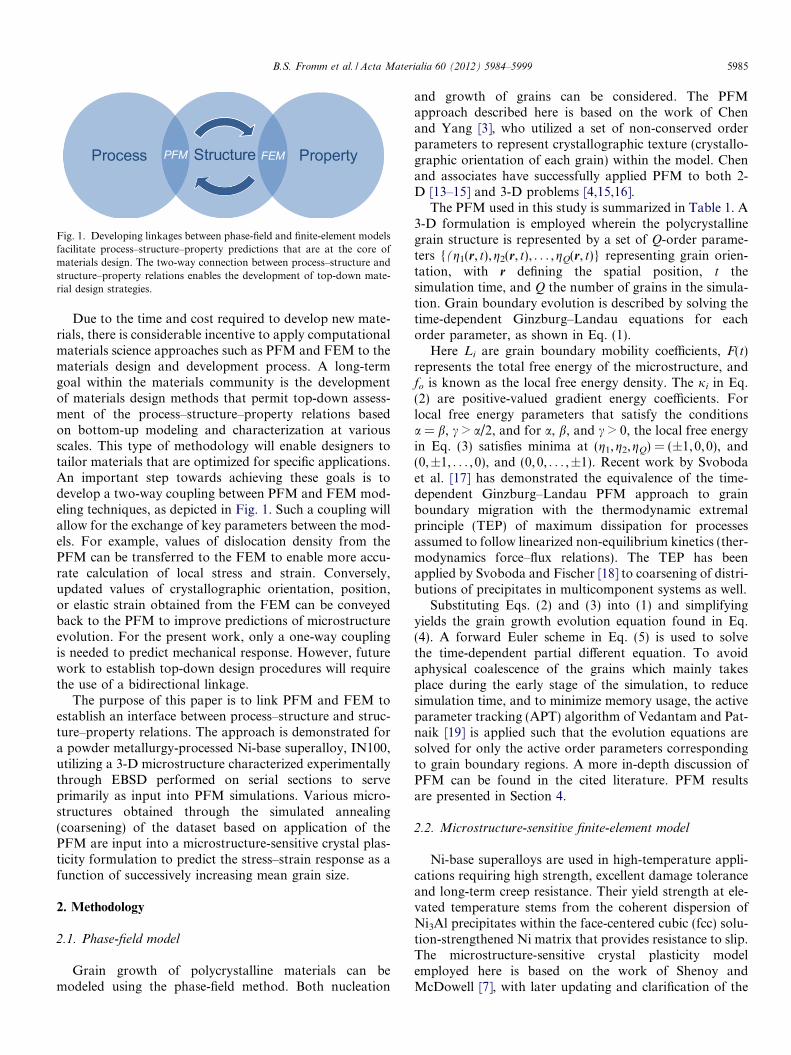
Available online at www.sciencedirect.com

www.elsevier.com/locate/actamat

Acta Materialia 60 (2012) 5984–5999

Linking phase-field and finite-element modeling forprocess–structure–property relations of a Ni-base superalloy

Bradley S. Fromm a,⇑, Kunok Chang b, David L. McDowell a,c, Long-Qing Chen b,Hamid Garmestani a

a School of Materials Science and Engineering, Georgia Institute of Technology, Atlanta, GA 30332, USAb Department of Materials Science and Engineering, The Pennsylvania State University, University Park, PA 16802, USAc The George W. Woodruff School of Mechanical Engineering, Georgia Institute of Technology, Atlanta, GA 30332, USA

Received 18 April 2012; received in revised form 25 June 2012; accepted 29 June 2012Available online 30 August 2012

Abstract

Establishing process–structure–property relationships is an important objective in the paradigm of materials design in order to reducethe time and cost needed to develop new materials. A method to link phase-field (process–structure relations) and microstructure-sen-sitive finite-element (structure–property relations) modeling is demonstrated for subsolvus polycrystalline IN100. A three-dimensionalexperimental dataset obtained by orientation imaging microscopy performed on serial sections is utilized to calibrate a phase-field modeland to calculate inputs for a finite-element analysis. Simulated annealing of the dataset realized through phase-field modeling results in arange of coarsened microstructures with varying grain size distributions that are each input into the finite-element model. A rate-depen-dent crystal plasticity constitutive model that captures the first-order effects of grain size, precipitate size and precipitate volume fractionon the mechanical response of IN100 at 650 �C is used to simulate stress–strain behavior of the coarsened polycrystals. Model limitationsand ideas for future work are discussed.� 2012 Acta Materialia Inc. Published by Elsevier Ltd. All rights reserved.

Keywords: Finite-element method; Crystal plasticity; Phase-field modeling; Process–structure–property relations; Microstructure-sensitive design

1. Introduction

Establishing process–structure–property relationships isessential in leveraging modeling and simulation to reducethe time and cost needed to develop new materials orimprove existing materials [1,2] and is at the core of materi-als design. Fig. 1 illustrates how the process–structure–prop-erty relationships form overlapping regions that representphysical couplings and transfer of related model informa-tion in materials design. Just as a material’s microstructureis coupled to the process path, its mechanical propertiesare directly correlated to the material microstructure.

Substantial progress has been made in connecting theprocess–structure–property relationships through advances

1359-6454/$36.00 � 2012 Acta Materialia Inc. Published by Elsevier Ltd. All

http://dx.doi.org/10.1016/j.actamat.2012.06.058

⇑ Corresponding author.E-mail address: [email protected] (B.S. Fromm).

in computational materials science and materials character-ization methods. For example, continuum mechanics-based techniques such as phase-field modeling (PFM)enable a direct linkage between the process–structure rela-tionships by simulating the nucleation and growth ofphases/grains within a material [3,4]. Likewise, microstruc-ture-sensitive finite-element modeling (FEM) facilitates thestructure–property correlation by predicting the aniso-tropic mechanical response of materials under thermome-chanical loading conditions, including the role ofmesoscopic microstructure morphology (e.g. grains,phases) [5–7]. Further advances in characterization tech-niques such as automated electron backscatter diffraction(EBSD) methods [8–10] and three-dimensional (3-D)X-ray diffraction [11,12] allow for digital representationof polycrystalline microstructures and facilitate calibrationof the computational models.

rights reserved.


mailto:[email protected]


Process PropertyStructurePFM FEM

Fig. 1. Developing linkages between phase-field and finite-element modelsfacilitate process–structure–property predictions that are at the core ofmaterials design. The two-way connection between process–structure andstructure–property relations enables the development of top-down mate-rial design strategies.

B.S. Fromm et al. / Acta Materialia 60 (2012) 5984–5999 5985

Due to the time and cost required to develop new mate-rials, there is considerable incentive to apply computationalmaterials science approaches such as PFM and FEM to thematerials design and development process. A long-termgoal within the materials community is the developmentof materials design methods that permit top-down assess-ment of the process–structure–property relations basedon bottom-up modeling and characterization at variousscales. This type of methodology will enable designers totailor materials that are optimized for specific applications.An important step towards achieving these goals is todevelop a two-way coupling between PFM and FEM mod-eling techniques, as depicted in Fig. 1. Such a coupling willallow for the exchange of key parameters between the mod-els. For example, values of dislocation density from thePFM can be transferred to the FEM to enable more accu-rate calculation of local stress and strain. Conversely,updated values of crystallographic orientation, position,or elastic strain obtained from the FEM can be conveyedback to the PFM to improve predictions of microstructureevolution. For the present work, only a one-way couplingis needed to predict mechanical response. However, futurework to establish top-down design procedures will requirethe use of a bidirectional linkage.

The purpose of this paper is to link PFM and FEM toestablish an interface between process–structure and struc-ture–property relations. The approach is demonstrated fora powder metallurgy-processed Ni-base superalloy, IN100,utilizing a 3-D microstructure characterized experimentallythrough EBSD performed on serial sections to serveprimarily as input into PFM simulations. Various micro-structures obtained through the simulated annealing(coarsening) of the dataset based on application of thePFM are input into a microstructure-sensitive crystal plas-ticity formulation to predict the stress–strain response as afunction of successively increasing mean grain size.

2. Methodology

2.1. Phase-field model

Grain growth of polycrystalline materials can bemodeled using the phase-field method. Both nucleation

and growth of grains can be considered. The PFMapproach described here is based on the work of Chenand Yang [3], who utilized a set of non-conserved orderparameters to represent crystallographic texture (crystallo-graphic orientation of each grain) within the model. Chenand associates have successfully applied PFM to both 2-D [13–15] and 3-D problems [4,15,16].

The PFM used in this study is summarized in Table 1. A3-D formulation is employed wherein the polycrystallinegrain structure is represented by a set of Q-order parame-ters {(g1(r, t),g2(r, t), . . . ,gQ(r, t)} representing grain orien-tation, with r defining the spatial position, t thesimulation time, and Q the number of grains in the simula-tion. Grain boundary evolution is described by solving thetime-dependent Ginzburg–Landau equations for eachorder parameter, as shown in Eq. (1).

Here Li are grain boundary mobility coefficients, F(t)represents the total free energy of the microstructure, andfo is known as the local free energy density. The ji in Eq.(2) are positive-valued gradient energy coefficients. Forlocal free energy parameters that satisfy the conditionsa = b, c > a/2, and for a, b, and c > 0, the local free energyin Eq. (3) satisfies minima at (g1,g2,gQ) = (±1,0,0), and(0,±1, . . . , 0), and (0, 0, . . . ,±1). Recent work by Svobodaet al. [17] has demonstrated the equivalence of the time-dependent Ginzburg–Landau PFM approach to grainboundary migration with the thermodynamic extremalprinciple (TEP) of maximum dissipation for processesassumed to follow linearized non-equilibrium kinetics (ther-modynamics force–flux relations). The TEP has beenapplied by Svoboda and Fischer [18] to coarsening of distri-butions of precipitates in multicomponent systems as well.

Substituting Eqs. (2) and (3) into (1) and simplifyingyields the grain growth evolution equation found in Eq.(4). A forward Euler scheme in Eq. (5) is used to solvethe time-dependent partial different equation. To avoidaphysical coalescence of the grains which mainly takesplace during the early stage of the simulation, to reducesimulation time, and to minimize memory usage, the activeparameter tracking (APT) algorithm of Vedantam and Pat-naik [19] is applied such that the evolution equations aresolved for only the active order parameters correspondingto grain boundary regions. A more in-depth discussion ofPFM can be found in the cited literature. PFM resultsare presented in Section 4.

2.2. Microstructure-sensitive finite-element model

Ni-base superalloys are used in high-temperature appli-cations requiring high strength, excellent damage toleranceand long-term creep resistance. Their yield strength at ele-vated temperature stems from the coherent dispersion ofNi3Al precipitates within the face-centered cubic (fcc) solu-tion-strengthened Ni matrix that provides resistance to slip.The microstructure-sensitive crystal plasticity modelemployed here is based on the work of Shenoy andMcDowell [7], with later updating and clarification of the

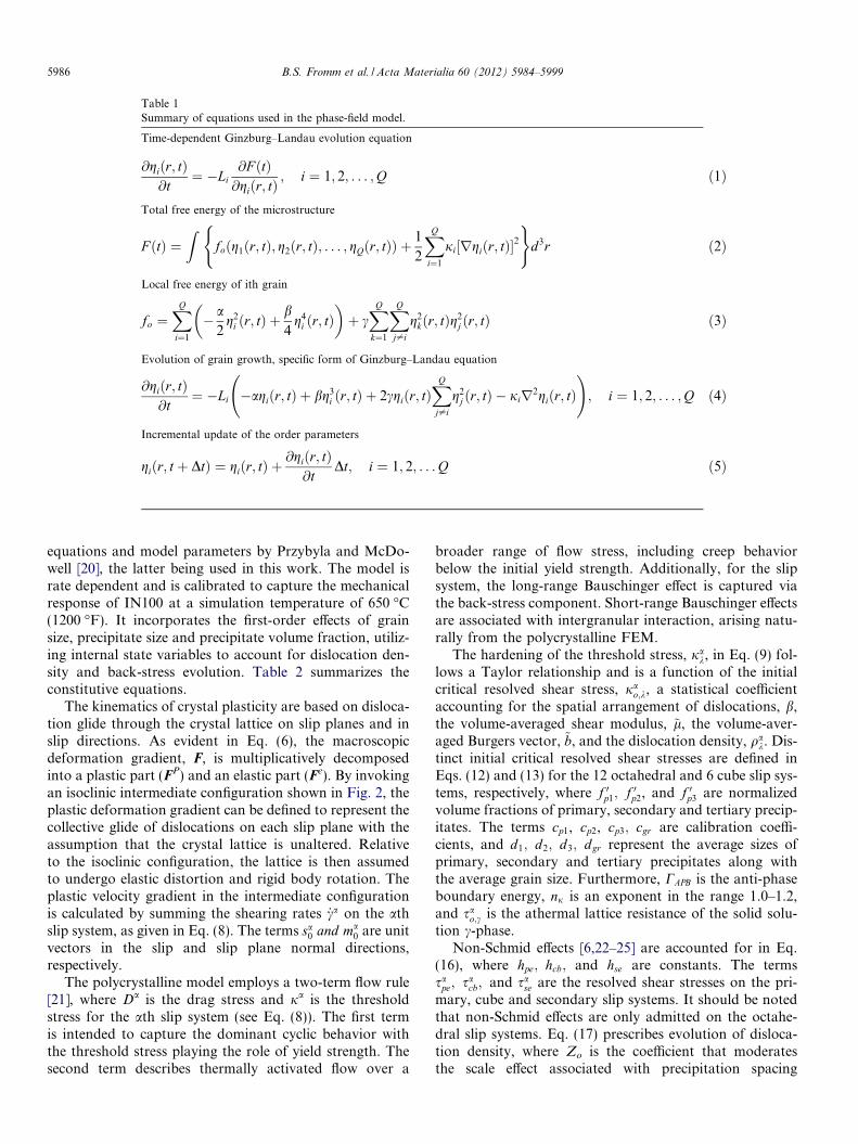
Table 1Summary of equations used in the phase-field model.

Time-dependent Ginzburg–Landau evolution equation

@giðr; tÞ@t

¼ �Li@F ðtÞ@giðr; tÞ

; i ¼ 1; 2; . . . ;Q ð1Þ

Total free energy of the microstructure

F ðtÞ ¼Z

foðg1ðr; tÞ; g2ðr; tÞ; . . . ; gQðr; tÞÞ þ1

2

XQ

i¼1

ji½rgiðr; tÞ�2

( )d3r ð2Þ

Local free energy of ith grain

fo ¼XQ

i¼1

� a2

g2i ðr; tÞ þ

b4

g4i ðr; tÞ

� �þ cXQ

k¼1

XQ

j–i

g2kðr; tÞg2

j ðr; tÞ ð3Þ

Evolution of grain growth, specific form of Ginzburg–Landau equation

@giðr; tÞ@t

¼ �Li �agiðr; tÞ þ bg3i ðr; tÞ þ 2cgiðr; tÞ

XQ

j–i

g2j ðr; tÞ � jir2giðr; tÞ

!; i ¼ 1; 2; . . . ;Q ð4Þ

Incremental update of the order parameters

giðr; t þ DtÞ ¼ giðr; tÞ þ@giðr; tÞ@t

Dt; i ¼ 1; 2; . . . Q ð5Þ

5986 B.S. Fromm et al. / Acta Materialia 60 (2012) 5984–5999

equations and model parameters by Przybyla and McDo-well [20], the latter being used in this work. The model israte dependent and is calibrated to capture the mechanicalresponse of IN100 at a simulation temperature of 650 �C(1200 �F). It incorporates the first-order effects of grainsize, precipitate size and precipitate volume fraction, utiliz-ing internal state variables to account for dislocation den-sity and back-stress evolution. Table 2 summarizes theconstitutive equations.

The kinematics of crystal plasticity are based on disloca-tion glide through the crystal lattice on slip planes and inslip directions. As evident in Eq. (6), the macroscopicdeformation gradient, F, is multiplicatively decomposedinto a plastic part (FP) and an elastic part (Fe). By invokingan isoclinic intermediate configuration shown in Fig. 2, theplastic deformation gradient can be defined to represent thecollective glide of dislocations on each slip plane with theassumption that the crystal lattice is unaltered. Relativeto the isoclinic configuration, the lattice is then assumedto undergo elastic distortion and rigid body rotation. Theplastic velocity gradient in the intermediate configurationis calculated by summing the shearing rates _ca on the athslip system, as given in Eq. (8). The terms sa

0 and ma0 are unit

vectors in the slip and slip plane normal directions,respectively.

The polycrystalline model employs a two-term flow rule[21], where Da is the drag stress and ja is the thresholdstress for the ath slip system (see Eq. (8)). The first termis intended to capture the dominant cyclic behavior withthe threshold stress playing the role of yield strength. Thesecond term describes thermally activated flow over a

broader range of flow stress, including creep behaviorbelow the initial yield strength. Additionally, for the slipsystem, the long-range Bauschinger effect is captured viathe back-stress component. Short-range Bauschinger effectsare associated with intergranular interaction, arising natu-rally from the polycrystalline FEM.

The hardening of the threshold stress, jak, in Eq. (9) fol-

lows a Taylor relationship and is a function of the initialcritical resolved shear stress, ja

o;k, a statistical coefficientaccounting for the spatial arrangement of dislocations, b,the volume-averaged shear modulus, ~l, the volume-aver-aged Burgers vector, ~b, and the dislocation density, qa

k. Dis-tinct initial critical resolved shear stresses are defined inEqs. (12) and (13) for the 12 octahedral and 6 cube slip sys-tems, respectively, where f 0p1; f 0p2, and f 0p3 are normalizedvolume fractions of primary, secondary and tertiary precip-itates. The terms cp1, cp2, cp3; cgr are calibration coeffi-cients, and d1; d2; d3; dgr represent the average sizes ofprimary, secondary and tertiary precipitates along withthe average grain size. Furthermore, CAPB is the anti-phaseboundary energy, nj is an exponent in the range 1.0–1.2,and sa

o;c is the athermal lattice resistance of the solid solu-tion c-phase.

Non-Schmid effects [6,22–25] are accounted for in Eq.(16), where hpe; hcb; and hse are constants. The termssa

pe; sacb; and sa

se are the resolved shear stresses on the pri-mary, cube and secondary slip systems. It should be notedthat non-Schmid effects are only admitted on the octahe-dral slip systems. Eq. (17) prescribes evolution of disloca-tion density, where Zo is the coefficient that moderatesthe scale effect associated with precipitation spacing

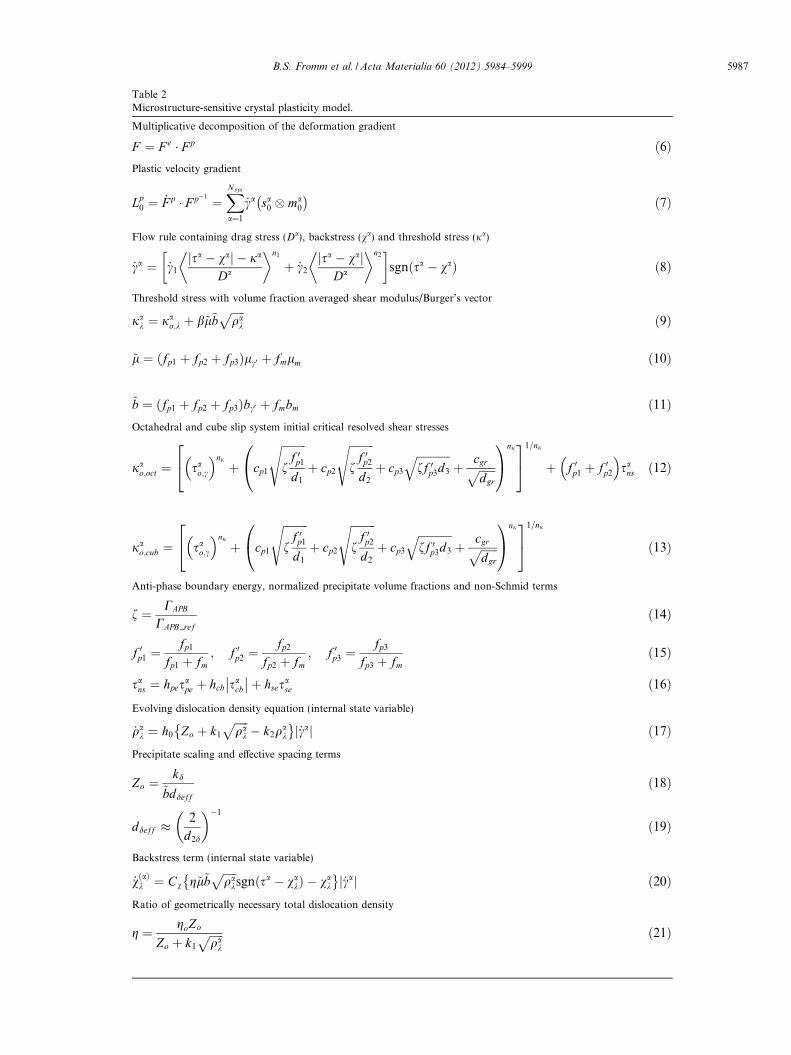
Table 2Microstructure-sensitive crystal plasticity model.

Multiplicative decomposition of the deformation gradient

F ¼ F e � F p ð6ÞPlastic velocity gradient

Lp0 ¼ _F p � F p�1 ¼

XNsys

a¼1

_ca sa0 � ma

0

� �ð7Þ

Flow rule containing drag stress (Da), backstress (va) and threshold stress (ja)

_ca ¼ _c1

jsa � vaj � ja

Da

� �n1

þ _c2

jsa � vajDa

� �n2�

sgnðsa � vaÞ ð8Þ

Threshold stress with volume fraction averaged shear modulus/Burger’s vector

jak ¼ ja

o;k þ b~l~bffiffiffiffiffiqa

k

pð9Þ

~l ¼ ðfp1 þ fp2 þ fp3Þlc0 þ fmlm ð10Þ

~b ¼ ðfp1 þ fp2 þ fp3Þbc0 þ fmbm ð11ÞOctahedral and cube slip system initial critical resolved shear stresses

jao;oct ¼ sa

o;c

� �nj

þ cp1

ffiffiffiffiffiffiffiffiffif

f 0p1

d1

sþ cp2


f 0p2

d2

sþ cp3

ffiffiffiffiffiffiffiffiffiffiffiffiff 0p3d3

qþ cgrffiffiffiffiffiffi

dgr

p0@

1A

nj24

35

1=nj

þ f 0p1 þ f 0p2

� �sa

ns ð12Þ

jao;cub ¼ sa

o;c

� �nj

þ cp1


f 0p1

d1

sþ cp2


f 0p2

d2

sþ cp3

ffiffiffiffiffiffiffiffiffiffiffiffiff 0p3d3

qþ cgrffiffiffiffiffiffi

dgr

p0@

1A

nj24

35

1=nj

ð13Þ

Anti-phase boundary energy, normalized precipitate volume fractions and non-Schmid terms

f ¼ CAPB

CAPB refð14Þ

f 0p1 ¼fp1

fp1 þ fm; f 0p2 ¼

fp2

fp2 þ fm; f 0p3 ¼

fp3

fp3 þ fmð15Þ

sans ¼ hpes

ape þ hcb sa

cb

þ hsesase ð16Þ

Evolving dislocation density equation (internal state variable)

_qak ¼ h0 Zo þ k1

ffiffiffiffiffiqa

k

p� k2q

ak

� �j _caj ð17Þ

Precipitate scaling and effective spacing terms

Zo ¼kd

~bddeff

ð18Þ

ddeff �2

d2d

� ��1

ð19Þ

Backstress term (internal state variable)

_vðaÞk ¼ Cv g~l~bffiffiffiffiffiqa

k

psgnðsa � va

kÞ � vak

� �j _caj ð20Þ

Ratio of geometrically necessary total dislocation density

g ¼ goZo

Zo þ k1

ffiffiffiffiffiqa

k

p ð21Þ


tertiary γ ’

secondary γ ’

carbides

primary γ ’

secondary γ ’

Fig. 3. TEM micrographs of IN100 microstructure from Ref. [30].

CurrentConfiguration

IntermediateConfiguration

ReferenceConfiguration

Fig. 2. Elastoplastic decomposition of the deformation gradient tensor.

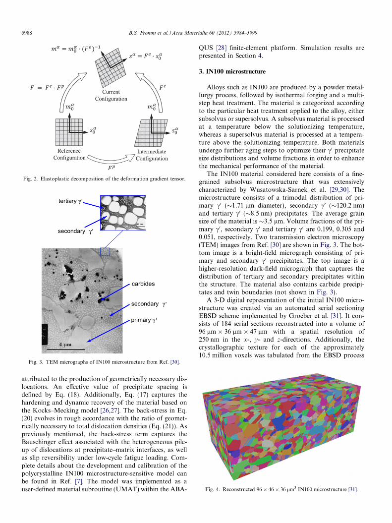
Fig. 4. Reconstructed 96 � 46 � 36 lm3 IN100 microstructure [31].


attributed to the production of geometrically necessary dis-locations. An effective value of precipitate spacing isdefined by Eq. (18). Additionally, Eq. (17) captures thehardening and dynamic recovery of the material based onthe Kocks–Mecking model [26,27]. The back-stress in Eq.(20) evolves in rough accordance with the ratio of geomet-rically necessary to total dislocation densities (Eq. (21)). Aspreviously mentioned, the back-stress term captures theBauschinger effect associated with the heterogeneous pile-up of dislocations at precipitate–matrix interfaces, as wellas slip reversibility under low-cycle fatigue loading. Com-plete details about the development and calibration of thepolycrystalline IN100 microstructure-sensitive model canbe found in Ref. [7]. The model was implemented as auser-defined material subroutine (UMAT) within the ABA-

QUS [28] finite-element platform. Simulation results arepresented in Section 4.

3. IN100 microstructure

Alloys such as IN100 are produced by a powder metal-lurgy process, followed by isothermal forging and a multi-step heat treatment. The material is categorized accordingto the particular heat treatment applied to the alloy, eithersubsolvus or supersolvus. A subsolvus material is processedat a temperature below the solutionizing temperature,whereas a supersolvus material is processed at a tempera-ture above the solutionizing temperature. Both materialsundergo further aging steps to optimize their c0 precipitatesize distributions and volume fractions in order to enhancethe mechanical performance of the material.

The IN100 material considered here consists of a fine-grained subsolvus microstructure that was extensivelycharacterized by Wusatowska-Sarnek et al. [29,30]. Themicrostructure consists of a trimodal distribution of pri-mary c0 (�1.71 lm diameter), secondary c0 (�120.2 nm)and tertiary c0 (�8.5 nm) precipitates. The average grainsize of the material is �3.5 lm. Volume fractions of the pri-mary c0, secondary c0 and tertiary c0 are 0.199, 0.305 and0.051, respectively. Two transmission electron microscopy(TEM) images from Ref. [30] are shown in Fig. 3. The bot-tom image is a bright-field micrograph consisting of pri-mary and secondary c0 precipitates. The top image is ahigher-resolution dark-field micrograph that captures thedistribution of tertiary and secondary precipitates withinthe structure. The material also contains carbide precipi-tates and twin boundaries (not shown in Fig. 3).

A 3-D digital representation of the initial IN100 micro-structure was created via an automated serial sectioningEBSD scheme implemented by Groeber et al. [31]. It con-sists of 184 serial sections reconstructed into a volume of96 lm � 36 lm � 47 lm with a spatial resolution of250 nm in the x-, y- and z-directions. Additionally, thecrystallographic texture for each of the approximately10.5 million voxels was tabulated from the EBSD process

0 1 2 3 4 5 6 7 8 9 10 11 12 130

0.05

0.10

0.15

0.20

0.25

0.30

0.35

0.40

Grain Size (μm)

Volu

me

Frac

tion

of G

rain

s

Experimental Data

Lognormal Fit

Gamma Fit

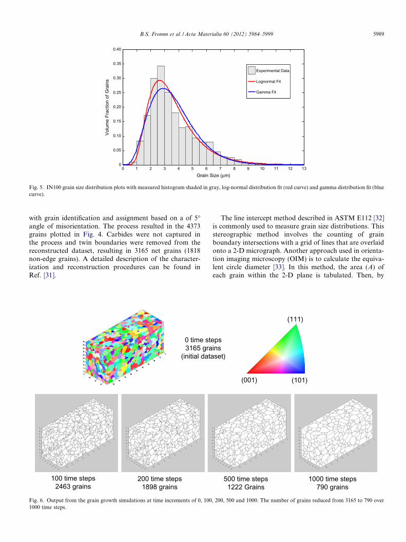
Fig. 5. IN100 grain size distribution plots with measured histogram shaded in gray, log-normal distribution fit (red curve) and gamma distribution fit (bluecurve).


with grain identification and assignment based on a of 5�angle of misorientation. The process resulted in the 4373grains plotted in Fig. 4. Carbides were not captured inthe process and twin boundaries were removed from thereconstructed dataset, resulting in 3165 net grains (1818non-edge grains). A detailed description of the character-ization and reconstruction procedures can be found inRef. [31].

0 time ste3165 gra

(initial data

100 time steps2463 grains


Fig. 6. Output from the grain growth simulations at time increments of 0, 1001000 time steps.

The line intercept method described in ASTM E112 [32]is commonly used to measure grain size distributions. Thisstereographic method involves the counting of grainboundary intersections with a grid of lines that are overlaidonto a 2-D micrograph. Another approach used in orienta-tion imaging microscopy (OIM) is to calculate the equiva-lent circle diameter [33]. In this method, the area (A) ofeach grain within the 2-D plane is tabulated. Then, by

psinsset)


500 time steps1222 Grains

(111)

(101)(001)

, 200, 500 and 1000. The number of grains reduced from 3165 to 790 over

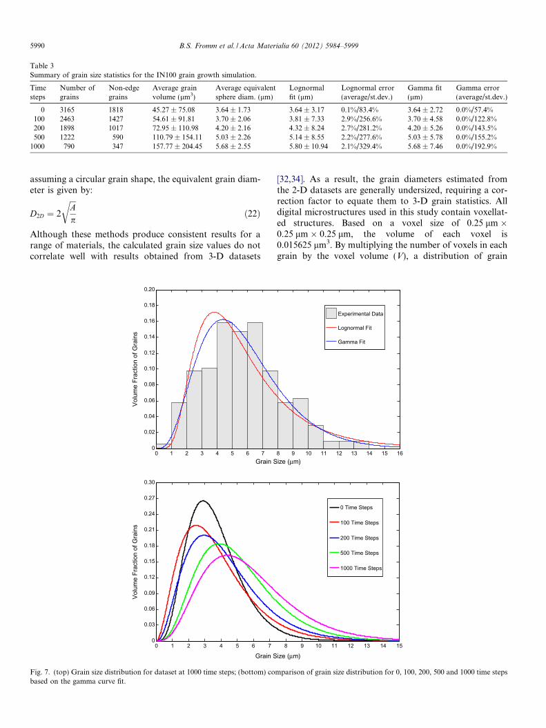
Table 3Summary of grain size statistics for the IN100 grain growth simulation.

Timesteps

Number ofgrains

Non-edgegrains

Average grainvolume (lm3)

Average equivalentsphere diam. (lm)

Lognormalfit (lm)

Lognormal error(average/st.dev.)

Gamma fit(lm)

Gamma error(average/st.dev.)

0 3165 1818 45.27 ± 75.08 3.64 ± 1.73 3.64 ± 3.17 0.1%/83.4% 3.64 ± 2.72 0.0%/57.4%100 2463 1427 54.61 ± 91.81 3.70 ± 2.06 3.81 ± 7.33 2.9%/256.6% 3.70 ± 4.58 0.0%/122.8%200 1898 1017 72.95 ± 110.98 4.20 ± 2.16 4.32 ± 8.24 2.7%/281.2% 4.20 ± 5.26 0.0%/143.5%500 1222 590 110.79 ± 154.11 5.03 ± 2.26 5.14 ± 8.55 2.2%/277.6% 5.03 ± 5.78 0.0%/155.2%

1000 790 347 157.77 ± 204.45 5.68 ± 2.55 5.80 ± 10.94 2.1%/329.4% 5.68 ± 7.46 0.0%/192.9%


assuming a circular grain shape, the equivalent grain diam-eter is given by:

D2D ¼ 2

ffiffiffiAp

rð22Þ

Although these methods produce consistent results for arange of materials, the calculated grain size values do notcorrelate well with results obtained from 3-D datasets

0 1 2 3 4 5 6 70

0.02

0.04

0.06

0.08

0.10

0.12

0.14

0.16

0.18

0.20

Grain S

Volu

me

Frac

tion

of G

rain

s

0 1 2 3 4 5 6 70

0.03

0.06

0.09

0.12

0.15

0.18

0.21

0.24

0.27

0.30

Grain S

Volu

me

Frac

tion

of G

rain

s

Fig. 7. (top) Grain size distribution for dataset at 1000 time steps; (bottom) cobased on the gamma curve fit.

[32,34]. As a result, the grain diameters estimated fromthe 2-D datasets are generally undersized, requiring a cor-rection factor to equate them to 3-D grain statistics. Alldigital microstructures used in this study contain voxellat-ed structures. Based on a voxel size of 0.25 lm �0.25 lm � 0.25 lm, the volume of each voxel is0.015625 lm3. By multiplying the number of voxels in eachgrain by the voxel volume (V), a distribution of grain

8 9 10 11 12 13 14 15 16ize (μm)

Experimental Data

Lognormal Fit

Gamma Fit

8 9 10 11 12 13 14 15

ize (μm)

0 Time Steps

100 Time Steps

200 Time Steps

500 Time Steps

1000 Time Steps

mparison of grain size distribution for 0, 100, 200, 500 and 1000 time steps

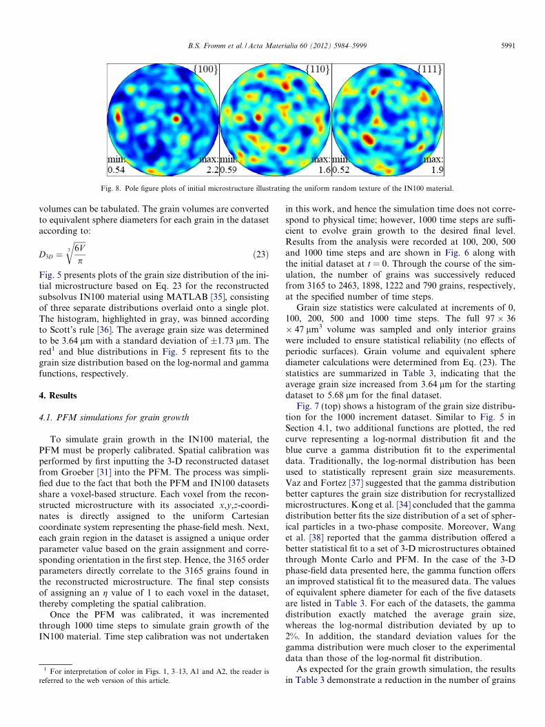
Fig. 8. Pole figure plots of initial microstructure illustrating the uniform random texture of the IN100 material.


volumes can be tabulated. The grain volumes are convertedto equivalent sphere diameters for each grain in the datasetaccording to:

D3D ¼ffiffiffiffiffiffi6Vp

3

rð23Þ

Fig. 5 presents plots of the grain size distribution of the ini-tial microstructure based on Eq. 23 for the reconstructedsubsolvus IN100 material using MATLAB [35], consistingof three separate distributions overlaid onto a single plot.The histogram, highlighted in gray, was binned accordingto Scott’s rule [36]. The average grain size was determinedto be 3.64 lm with a standard deviation of ±1.73 lm. Thered1 and blue distributions in Fig. 5 represent fits to thegrain size distribution based on the log-normal and gammafunctions, respectively.

4. Results

4.1. PFM simulations for grain growth

To simulate grain growth in the IN100 material, thePFM must be properly calibrated. Spatial calibration wasperformed by first inputting the 3-D reconstructed datasetfrom Groeber [31] into the PFM. The process was simpli-fied due to the fact that both the PFM and IN100 datasetsshare a voxel-based structure. Each voxel from the recon-structed microstructure with its associated x,y,z-coordi-nates is directly assigned to the uniform Cartesiancoordinate system representing the phase-field mesh. Next,each grain region in the dataset is assigned a unique orderparameter value based on the grain assignment and corre-sponding orientation in the first step. Hence, the 3165 orderparameters directly correlate to the 3165 grains found inthe reconstructed microstructure. The final step consistsof assigning an g value of 1 to each voxel in the dataset,thereby completing the spatial calibration.

Once the PFM was calibrated, it was incrementedthrough 1000 time steps to simulate grain growth of theIN100 material. Time step calibration was not undertaken

1 For interpretation of color in Figs. 1, 3–13, A1 and A2, the reader isreferred to the web version of this article.

in this work, and hence the simulation time does not corre-spond to physical time; however, 1000 time steps are suffi-cient to evolve grain growth to the desired final level.Results from the analysis were recorded at 100, 200, 500and 1000 time steps and are shown in Fig. 6 along withthe initial dataset at t = 0. Through the course of the sim-ulation, the number of grains was successively reducedfrom 3165 to 2463, 1898, 1222 and 790 grains, respectively,at the specified number of time steps.

Grain size statistics were calculated at increments of 0,100, 200, 500 and 1000 time steps. The full 97 � 36� 47 lm3 volume was sampled and only interior grainswere included to ensure statistical reliability (no effects ofperiodic surfaces). Grain volume and equivalent spherediameter calculations were determined from Eq. (23). Thestatistics are summarized in Table 3, indicating that theaverage grain size increased from 3.64 lm for the startingdataset to 5.68 lm for the final dataset.

Fig. 7 (top) shows a histogram of the grain size distribu-tion for the 1000 increment dataset. Similar to Fig. 5 inSection 4.1, two additional functions are plotted, the redcurve representing a log-normal distribution fit and theblue curve a gamma distribution fit to the experimentaldata. Traditionally, the log-normal distribution has beenused to statistically represent grain size measurements.Vaz and Fortez [37] suggested that the gamma distributionbetter captures the grain size distribution for recrystallizedmicrostructures. Kong et al. [34] concluded that the gammadistribution better fits the size distribution of a set of spher-ical particles in a two-phase composite. Moreover, Wanget al. [38] reported that the gamma distribution offered abetter statistical fit to a set of 3-D microstructures obtainedthrough Monte Carlo and PFM. In the case of the 3-Dphase-field data presented here, the gamma function offersan improved statistical fit to the measured data. The valuesof equivalent sphere diameter for each of the five datasetsare listed in Table 3. For each of the datasets, the gammadistribution exactly matched the average grain size,whereas the log-normal distribution deviated by up to2%. In addition, the standard deviation values for thegamma distribution were much closer to the experimentaldata than those of the log-normal fit distribution.

As expected for the grain growth simulation, the resultsin Table 3 demonstrate a reduction in the number of grains

20x20x20 µm3

15x15x15 µm3

10x10x10 µm3

5x5x5 µm3

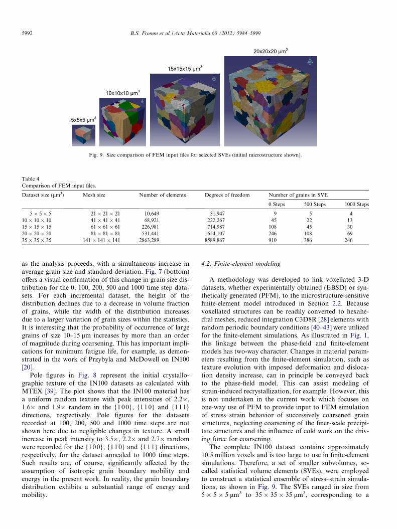
Fig. 9. Size comparison of FEM input files for selected SVEs (initial microstructure shown).

Table 4Comparison of FEM input files.

Dataset size (lm3) Mesh size Number of elements Degrees of freedom Number of grains in SVE

0 Steps 500 Steps 1000 Steps

5 � 5 � 5 21 � 21 � 21 10,649 31,947 9 5 410 � 10 � 10 41 � 41 � 41 68,921 222,267 45 22 1315 � 15 � 15 61 � 61 � 61 226,981 714,987 108 45 3020 � 20 � 20 81 � 81 � 81 531,441 1654,107 246 108 6935 � 35 � 35 141 � 141 � 141 2863,289 8589,867 910 386 246


as the analysis proceeds, with a simultaneous increase inaverage grain size and standard deviation. Fig. 7 (bottom)offers a visual confirmation of this change in grain size dis-tribution for the 0, 100, 200, 500 and 1000 time step data-sets. For each incremental dataset, the height of thedistribution declines due to a decrease in volume fractionof grains, while the width of the distribution increasesdue to a larger variation of grain sizes within the statistics.It is interesting that the probability of occurrence of largegrains of size 10–15 lm increases by more than an orderof magnitude during coarsening. This has important impli-cations for minimum fatigue life, for example, as demon-strated in the work of Przybyla and McDowell on IN100[20].

Pole figures in Fig. 8 represent the initial crystallo-graphic texture of the IN100 datasets as calculated withMTEX [39]. The plot shows that the IN100 material hasa uniform random texture with peak intensities of 2.2�,1.6� and 1.9� random in the {100}, {110} and {111}directions, respectively. Pole figures for the datasetsrecorded at 100, 200, 500 and 1000 time steps are notshown here due to negligible changes in texture. A smallincrease in peak intensity to 3.5�, 2.2� and 2.7� randomwere recorded for the {100}, {110} and {111} directions,respectively, for the dataset annealed to 1000 time steps.Such results are, of course, significantly affected by theassumption of isotropic grain boundary mobility andenergy in the present work. In reality, the grain boundarydistribution exhibits a substantial range of energy andmobility.

4.2. Finite-element modeling

A methodology was developed to link voxellated 3-Ddatasets, whether experimentally obtained (EBSD) or syn-thetically generated (PFM), to the microstructure-sensitivefinite-element model introduced in Section 2.2. Becausevoxellated structures can be readily converted to hexahe-dral meshes, reduced integration C3D8R [28] elements withrandom periodic boundary conditions [40–43] were utilizedfor the finite-element simulations. As illustrated in Fig. 1,this linkage between the phase-field and finite-elementmodels has two-way character. Changes in material param-eters resulting from the finite-element simulation, such astexture evolution with imposed deformation and disloca-tion density increase, can in principle be conveyed backto the phase-field model. This can assist modeling ofstrain-induced recrystallization, for example. However, thisis not undertaken in the current work which focuses onone-way use of PFM to provide input to FEM simulationof stress–strain behavior of successively coarsened grainstructures, neglecting coarsening of the finer-scale precipi-tate structures and the influence of cold work on the driv-ing force for coarsening.

The complete IN100 dataset contains approximately10.5 million voxels and is too large to use in finite-elementsimulations. Therefore, a set of smaller subvolumes, so-called statistical volume elements (SVEs), were employedto construct a statistical ensemble of stress–strain simula-tions, as shown in Fig. 9. The SVEs ranged in size from5 � 5 � 5 lm3 to 35 � 35 � 35 lm3, corresponding to a

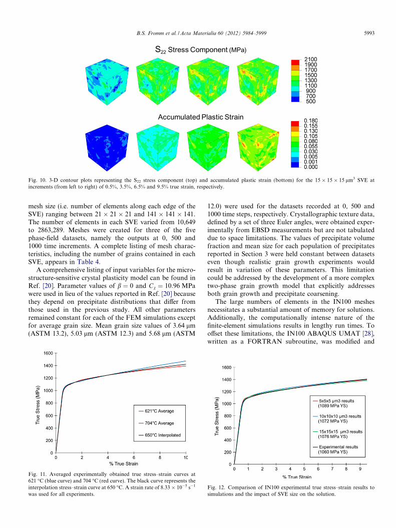
Fig. 10. 3-D contour plots representing the S22 stress component (top) and accumulated plastic strain (bottom) for the 15 � 15 � 15 lm3 SVE atincrements (from left to right) of 0.5%, 3.5%, 6.5% and 9.5% true strain, respectively.


mesh size (i.e. number of elements along each edge of theSVE) ranging between 21 � 21 � 21 and 141 � 141 � 141.The number of elements in each SVE varied from 10,649to 2863,289. Meshes were created for three of the fivephase-field datasets, namely the outputs at 0, 500 and1000 time increments. A complete listing of mesh charac-teristics, including the number of grains contained in eachSVE, appears in Table 4.

A comprehensive listing of input variables for the micro-structure-sensitive crystal plasticity model can be found inRef. [20]. Parameter values of b ¼ 0 and Cv ¼ 10:96 MPawere used in lieu of the values reported in Ref. [20] becausethey depend on precipitate distributions that differ fromthose used in the previous study. All other parametersremained constant for each of the FEM simulations exceptfor average grain size. Mean grain size values of 3.64 lm(ASTM 13.2), 5.03 lm (ASTM 12.3) and 5.68 lm (ASTM

Fig. 11. Averaged experimentally obtained true stress–strain curves at621 �C (blue curve) and 704 �C (red curve). The black curve represents theinterpolation stress–strain curve at 650 �C. A strain rate of 8.33 � 10�5 s�1

was used for all experiments.

12.0) were used for the datasets recorded at 0, 500 and1000 time steps, respectively. Crystallographic texture data,defined by a set of three Euler angles, were obtained exper-imentally from EBSD measurements but are not tabulateddue to space limitations. The values of precipitate volumefraction and mean size for each population of precipitatesreported in Section 3 were held constant between datasetseven though realistic grain growth experiments wouldresult in variation of these parameters. This limitationcould be addressed by the development of a more complextwo-phase grain growth model that explicitly addressesboth grain growth and precipitate coarsening.

The large numbers of elements in the IN100 meshesnecessitates a substantial amount of memory for solutions.Additionally, the computationally intense nature of thefinite-element simulations results in lengthy run times. Tooffset these limitations, the IN100 ABAQUS UMAT [28],written as a FORTRAN subroutine, was modified and

Fig. 12. Comparison of IN100 experimental true stress–strain results tosimulations and the impact of SVE size on the solution.

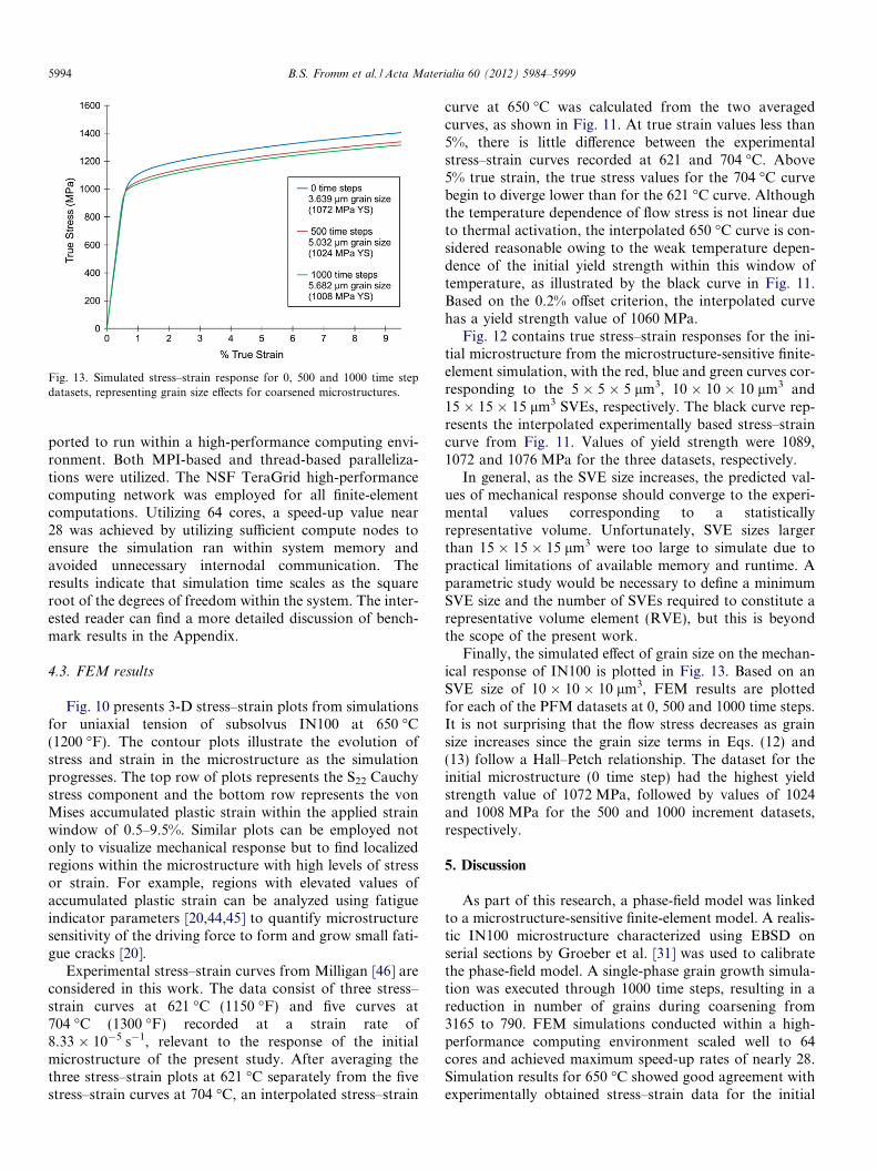
Fig. 13. Simulated stress–strain response for 0, 500 and 1000 time stepdatasets, representing grain size effects for coarsened microstructures.


ported to run within a high-performance computing envi-ronment. Both MPI-based and thread-based paralleliza-tions were utilized. The NSF TeraGrid high-performancecomputing network was employed for all finite-elementcomputations. Utilizing 64 cores, a speed-up value near28 was achieved by utilizing sufficient compute nodes toensure the simulation ran within system memory andavoided unnecessary internodal communication. Theresults indicate that simulation time scales as the squareroot of the degrees of freedom within the system. The inter-ested reader can find a more detailed discussion of bench-mark results in the Appendix.

4.3. FEM results

Fig. 10 presents 3-D stress–strain plots from simulationsfor uniaxial tension of subsolvus IN100 at 650 �C(1200 �F). The contour plots illustrate the evolution ofstress and strain in the microstructure as the simulationprogresses. The top row of plots represents the S22 Cauchystress component and the bottom row represents the vonMises accumulated plastic strain within the applied strainwindow of 0.5–9.5%. Similar plots can be employed notonly to visualize mechanical response but to find localizedregions within the microstructure with high levels of stressor strain. For example, regions with elevated values ofaccumulated plastic strain can be analyzed using fatigueindicator parameters [20,44,45] to quantify microstructuresensitivity of the driving force to form and grow small fati-gue cracks [20].

Experimental stress–strain curves from Milligan [46] areconsidered in this work. The data consist of three stress–strain curves at 621 �C (1150 �F) and five curves at704 �C (1300 �F) recorded at a strain rate of8.33 � 10�5 s�1, relevant to the response of the initialmicrostructure of the present study. After averaging thethree stress–strain plots at 621 �C separately from the fivestress–strain curves at 704 �C, an interpolated stress–strain

curve at 650 �C was calculated from the two averagedcurves, as shown in Fig. 11. At true strain values less than5%, there is little difference between the experimentalstress–strain curves recorded at 621 and 704 �C. Above5% true strain, the true stress values for the 704 �C curvebegin to diverge lower than for the 621 �C curve. Althoughthe temperature dependence of flow stress is not linear dueto thermal activation, the interpolated 650 �C curve is con-sidered reasonable owing to the weak temperature depen-dence of the initial yield strength within this window oftemperature, as illustrated by the black curve in Fig. 11.Based on the 0.2% offset criterion, the interpolated curvehas a yield strength value of 1060 MPa.

Fig. 12 contains true stress–strain responses for the ini-tial microstructure from the microstructure-sensitive finite-element simulation, with the red, blue and green curves cor-responding to the 5 � 5 � 5 lm3, 10 � 10 � 10 lm3 and15 � 15 � 15 lm3 SVEs, respectively. The black curve rep-resents the interpolated experimentally based stress–straincurve from Fig. 11. Values of yield strength were 1089,1072 and 1076 MPa for the three datasets, respectively.

In general, as the SVE size increases, the predicted val-ues of mechanical response should converge to the experi-mental values corresponding to a statisticallyrepresentative volume. Unfortunately, SVE sizes largerthan 15 � 15 � 15 lm3 were too large to simulate due topractical limitations of available memory and runtime. Aparametric study would be necessary to define a minimumSVE size and the number of SVEs required to constitute arepresentative volume element (RVE), but this is beyondthe scope of the present work.

Finally, the simulated effect of grain size on the mechan-ical response of IN100 is plotted in Fig. 13. Based on anSVE size of 10 � 10 � 10 lm3, FEM results are plottedfor each of the PFM datasets at 0, 500 and 1000 time steps.It is not surprising that the flow stress decreases as grainsize increases since the grain size terms in Eqs. (12) and(13) follow a Hall–Petch relationship. The dataset for theinitial microstructure (0 time step) had the highest yieldstrength value of 1072 MPa, followed by values of 1024and 1008 MPa for the 500 and 1000 increment datasets,respectively.

5. Discussion

As part of this research, a phase-field model was linkedto a microstructure-sensitive finite-element model. A realis-tic IN100 microstructure characterized using EBSD onserial sections by Groeber et al. [31] was used to calibratethe phase-field model. A single-phase grain growth simula-tion was executed through 1000 time steps, resulting in areduction in number of grains during coarsening from3165 to 790. FEM simulations conducted within a high-performance computing environment scaled well to 64cores and achieved maximum speed-up rates of nearly 28.Simulation results for 650 �C showed good agreement withexperimentally obtained stress–strain data for the initial


microstructure. A discussion of the limitations, approxima-tions and suggestions for future research related to thephase-field model, material characterization, and finite-ele-ment model follows below.

The phase-field model utilized in this study was based ona binary Ni–Al system. Augmentation of the model toallow for additional alloy elements in the thermodynamiccalculations would improve applicability of the graingrowth results. Additionally, the current PFM does notconsider the effect of depleted zones on precipitate forma-tion/growth or account for inclusion of hard phases withinthe matrix or along grain boundaries that are known toaffect fatigue life and grain boundary mobility within Ni-base superalloys. Recently, Chang et al. [15] utilizedPFM to study the ability of second-phase particles to inhi-bit grain boundary migration. Although the model used inthis research was calibrated spatially from an experimen-tally characterized microstructure, the issue of time calibra-tion to better correlate the model to known process pathhistories needs to be addressed. Lastly, development of atwo-phase grain growth model (c�c0) to enable the simul-taneous coarsening of both c0 precipitates and grains iswarranted.

Experimental characterization of the IN100 microstruc-ture is critical to the calibration of both the phase-field andfinite-element models, serving as the basis for the realisticgrain structures presented here. A limitation of the existingIN100 dataset is the absence of twin boundaries within thereconstructed microstructure. Because the subsolvus IN100twins were similar in width to the scan resolution, theycould not be properly recovered and were thus removedfrom the dataset [31]. However, twin boundaries are knownto affect the mechanical properties of metals as they effec-tively reduce the grain size of the structure and provide bar-riers for dislocation migration, thus influencing the fatigueresponse of the material. Utilizing higher-resolution EBSDscans would allow for more accurate recovery and recon-struction of the twin boundaries.

The FEM approach does not fully address the role ofgrain boundary structure on dislocation slip transferbetween grains. Rohrer et al. [47,48] have devoted signifi-cant efforts to reconstructing grain boundary networksfrom 3-D EBSD datasets and calculating the associateddistribution of grain boundary character and grain bound-ary energy within the microstructure, which can providevaluable input into PFM simulations and enhanced FEMsimulations that employ constitutive equations for sliptransfer at grain boundaries.

Wilkinson and colleagues [49] have described a methodto accurately determine the full elastic strain tensor fromEBSD scan data. This elastic strain tensor is beneficialfor both calibrating and verifying finite element models.Adams et al. [50,51] augmented the technique by generat-ing synthetic strain-free electron backscatter patterns forpurposes of cross-correlation and estimated values of lat-tice curvature and dislocation density in addition to elasticstrain. Generating 3-D maps of dislocation density for a

given EBSD dataset would improve the accuracy of FEMresults since the simulation could be calibrated to experi-ments with regard to dislocation density evolution.

Microstructure-sensitive FEM requires continuedresearch in several areas. Recently, McDowell [52] dis-cussed key challenges for future progress, including: mod-eling over multiple length scales, statistical behavior ofdislocations and formation of subgrains, multiscale kine-matics, treatment of grain boundaries, and a discussionof top-down vs. bottom-up modeling schemes. He furtherelaborated on the need to advance discrete dislocationand crystal plasticity theory within the context of concur-rent and hierarchical multiscale modeling strategies [53].Several areas that may impact future FEM developmentare as follows:

(i) The concept of minimum SVE size and number ofSVEs required to simulate an RVE requires furtherdevelopment. As argued by Fullwood et al. [54], theergodic assumption must be invoked when using anensemble of SVEs to fit an RVE. This requires thatthe statistical average of the desired property withinthe SVEs must be equivalent to the statistics for theRVE. The goal in selecting an SVE size is to minimizethe average error and standard deviation between thechosen set of SVEs and the RVE, and simultaneouslyto minimize SVE size. Unfortunately, these two fac-tors are in direct competition since the SVE size mustbe increased in order to reduce error. Utilizing two-point statistics, Niezgoda and coworkers [55] illus-trated a procedure to determine the appropriateSVE size for both a two-phase composite and a poly-crystalline metal. McDowell et al. [56] have elabo-rated on the use of a statistically equivalent RVE(SERVE) for general problems without phase rear-rangement/damage and RVE sets for more complexproblems that include evolution of damage withinthe microstructure.

(ii) Recent work by Przybyla and McDowell [20] con-cluded that as few as 25 SVEs were sufficient to fitan extreme value distribution of the Fatemi–Sociefatigue indicator parameter at 97% confidence utiliz-ing a 28 � 28 � 28 element mesh containing 77grains. Further, they concluded that the primary zoneof influence on any given grain extended to the twonearest neighbors of the grain, assuming periodicboundary conditions are imposed in the simulation.Additionally, it was observed that the extreme valuefatigue indicator parameter did not vary substantiallyfor edges with 12 or more elements along the edge.Based on these conclusions, an SVE volume size con-taining 20–30 elements and 5 grains per edge shouldbe sufficient to conduct a parametric study for theresearch presented here. From Table 4, this corre-sponds to an intermediate SVE size between10 � 10 � 10 lm3 and 15 � 15 � 15 lm3 to ensure asufficient number of grains, but a SVE size between

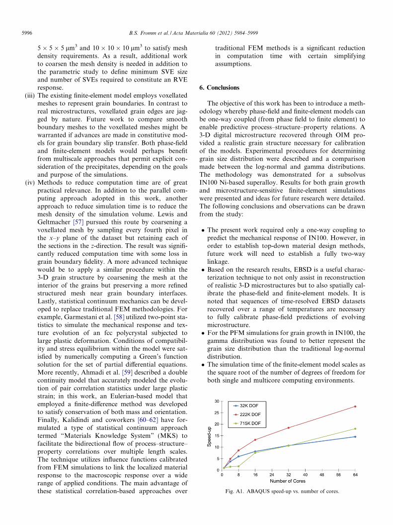
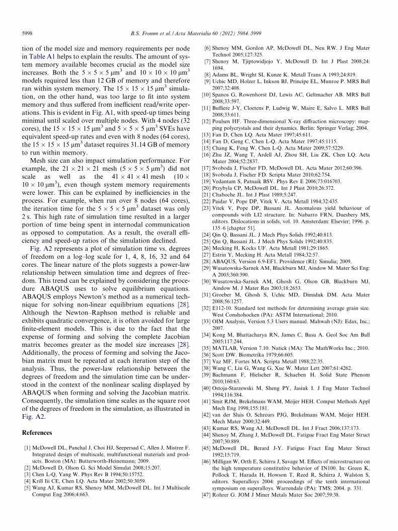
Fig. A1. ABAQUS speed-up vs. number of cores.


5 � 5 � 5 lm3 and 10 � 10 � 10 lm3 to satisfy meshdensity requirements. As a result, additional workto coarsen the mesh density is needed in addition tothe parametric study to define minimum SVE sizeand number of SVEs required to constitute an RVEresponse.

(iii) The existing finite-element model employs voxellatedmeshes to represent grain boundaries. In contrast toreal microstructures, voxellated grain edges are jag-ged by nature. Future work to compare smoothboundary meshes to the voxellated meshes might bewarranted if advances are made in constitutive mod-els for grain boundary slip transfer. Both phase-fieldand finite-element models would perhaps benefitfrom multiscale approaches that permit explicit con-sideration of the precipitates, depending on the goalsand purpose of the simulations.

(iv) Methods to reduce computation time are of greatpractical relevance. In addition to the parallel com-puting approach adopted in this work, anotherapproach to reduce simulation time is to reduce themesh density of the simulation volume. Lewis andGeltmacher [57] pursued this route by coarsening avoxellated mesh by sampling every fourth pixel inthe x–y plane of the dataset but retaining each ofthe sections in the z-direction. The result was signifi-cantly reduced computation time with some loss ingrain boundary fidelity. A more advanced techniquewould be to apply a similar procedure within the3-D grain structure by coarsening the mesh at theinterior of the grains but preserving a more refinedstructured mesh near grain boundary interfaces.Lastly, statistical continuum mechanics can be devel-oped to replace traditional FEM methodologies. Forexample, Garmestani et al. [58] utilized two-point sta-tistics to simulate the mechanical response and tex-ture evolution of an fcc polycrystal subjected tolarge plastic deformation. Conditions of compatibil-ity and stress equilibrium within the model were sat-isfied by numerically computing a Green’s functionsolution for the set of partial differential equations.More recently, Ahmadi et al. [59] described a doublecontinuity model that accurately modeled the evolu-tion of pair correlation statistics under large plasticstrain; in this work, an Eulerian-based model thatemployed a finite-difference method was developedto satisfy conservation of both mass and orientation.Finally, Kalidindi and coworkers [60–62] have for-mulated a type of statistical continuum approachtermed “Materials Knowledge System” (MKS) tofacilitate the bidirectional flow of process–structure–property correlations over multiple length scales.The technique utilizes influence functions calibratedfrom FEM simulations to link the localized materialresponse to the macroscopic response over a widerange of applied conditions. The main advantage ofthese statistical correlation-based approaches over

traditional FEM methods is a significant reductionin computation time with certain simplifyingassumptions.

6. Conclusions

The objective of this work has been to introduce a meth-odology whereby phase-field and finite-element models canbe one-way coupled (from phase field to finite element) toenable predictive process–structure–property relations. A3-D digital microstructure recovered through OIM pro-vided a realistic grain structure necessary for calibrationof the models. Experimental procedures for determininggrain size distribution were described and a comparisonmade between the log-normal and gamma distributions.The methodology was demonstrated for a subsolvusIN100 Ni-based superalloy. Results for both grain growthand microstructure-sensitive finite-element simulationswere presented and ideas for future research were detailed.The following conclusions and observations can be drawnfrom the study:

The present work required only a one-way coupling topredict the mechanical response of IN100. However, inorder to establish top-down material design methods,future work will need to establish a fully two-waylinkage. Based on the research results, EBSD is a useful charac-

terization technique to not only assist in reconstructionof realistic 3-D microstructures but to also spatially cal-ibrate the phase-field and finite-element models. It isnoted that sequences of time-resolved EBSD datasetsrecovered over a range of temperatures are necessaryto fully calibrate phase-field predictions of evolvingmicrostructure. For the PFM simulations for grain growth in IN100, the

gamma distribution was found to better represent thegrain size distribution than the traditional log-normaldistribution. The simulation time of the finite-element model scales as

the square root of the number of degrees of freedom forboth single and multicore computing environments.

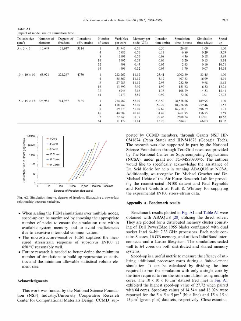
Table A1Impact of model size on simulation time.

Dataset size(lm3)

Number ofelements

Degrees offreedom

Iterations(6% strain)

Numberof cores

Variablesper core

Memory pernode (GB)

Iterationtime (min)

Simulationtime (hours)

Simulationtime (days)

Speed-up

5 � 5 � 5 10,649 31,947 3114 1 31,947 0.76 0.50 26.08 1.09 1.004 7987 0.76 0.13 6.89 0.29 3.798 3993 0.76 0.08 4.36 0.18 5.99

16 1997 0.54 0.06 3.20 0.13 8.1432 998 0.43 0.05 2.43 0.10 10.7164 499 0.32 0.03 1.79 0.07 14.54

10 � 10 � 10 68,921 222,267 4730 1 222,267 11.12 25.41 2002.89 83.45 1.004 55,567 11.12 5.17 407.83 16.99 4.918 27,783 11.12 2.95 232.30 9.68 8.62

16 13,892 7.97 1.92 151.62 6.32 13.2132 6946 7.16 1.38 108.79 4.53 18.4164 3473 5.89 0.92 72.26 3.01 27.72

15 � 15 � 15 226,981 714,987 7185 1 714,987 55.07 238.50 28,558.86 1189.95 1.004 178,747 55.07 152.22 18,226.98 759.46 1.578 89,373 55.07 139.62 16,718.21 696.59 1.71

16 44,687 40.40 31.42 3761.95 156.75 7.5932 22,343 38.37 22.45 2688.24 112.01 10.6264 11,172 31.14 13.23 1584.61 66.03 18.02

Fig. A2. Simulation time vs. degrees of freedom, illustrating a power-lawrelationship between variables.


When scaling the FEM simulations over multiple nodes,speed-up can be maximized by choosing the appropriatenumber of nodes to ensure the simulation runs withinavailable system memory and to avoid inefficienciesdue to excessive internodal communication. The microstructure-sensitive FEM captures the mea-

sured stressstrain response of subsolvus IN100 at650 �C reasonably well. Future research is needed to better define the minimum

number of simulations to build up representative statis-tics and the minimum allowable statistical volume ele-ment size.

Acknowledgments

This work was funded by the National Science Founda-tion (NSF) Industry/University Cooperative ResearchCenter for Computational Materials Design (CCMD) sup-

ported by CCMD members, through Grants NSF IIP-0541674 (Penn State) and IIP-541678 (Georgia Tech).The research was also supported in part by the NationalScience Foundation through TeraGrid resources providedby The National Center for Supercomputing Applications(NCSA), under grant no. TG-MSS090045. The authorswould like to specifically acknowledge the assistance ofDr. Seid Koric for help in running ABAQUS at NCSA.Additionally, we recognize Dr. Michael Groeber and Dr.Michael Uchic of the Air Force Research Lab for provid-ing the reconstructed IN100 dataset and Paul Reynoldsand Robert Grelotti at Pratt & Whitney for supplyingthe experimental IN100 stress–strain data.

Appendix A. Benchmark results

Benchmark results plotted in Fig. A1 and Table A1 wereobtained with ABAQUS [28] utilizing the direct solver.They are plotted for a distributed memory cluster consist-ing of Dell PowerEdge 1955 blades configured with dualsocket Intel 64-bit 2.33 GHz processors. Each node con-tains 8 cores, 16 GB memory, and utilizes InfiniBand inter-connects and a Lustre filesystem. The simulations scaledwell to 64 cores on both distributed and shared memorysystems.

Speed-up is a useful metric to measure the efficacy of uti-lizing additional processor cores during a finite-elementsimulation. It can be calculated by dividing the timerequired to run the simulation with only a single core bythe time required to run the same simulation using multiplecores. The 10 � 10 � 10 lm3 dataset (red line) in Fig. A1exhibited the highest speed-up value of 27.72 when pairedwith 64 cores. Speed-up values of 14.54� and 18.02� werereported for the 5 � 5 � 5 lm3 (blue line) and 15 � 15 �15 lm3 (green plot) datasets, respectively. Close examina-


tion of the model size and memory requirements per nodein Table A1 helps to explain the results. The amount of sys-tem memory available becomes crucial as the model sizeincreases. Both the 5 � 5 � 5 lm3 and 10 � 10 � 10 lm3

models required less than 12 GB of memory and thereforeran within system memory. The 15 � 15 � 15 lm3 simula-tion, on the other hand, was too large to fit into systemmemory and thus suffered from inefficient read/write oper-ations. This is evident in Fig. A1, with speed-up times beingminimal until scaled over multiple nodes. With 4 nodes (32cores), the 15 � 15 � 15 lm3 and 5 � 5 � 5 lm3 SVEs haveequivalent speed-up rates and even with 8 nodes (64 cores),the 15 � 15 � 15 lm3 dataset requires 31.14 GB of memoryto run within memory.

Mesh size can also impact simulation performance. Forexample, the 21 � 21 � 21 mesh (5 � 5 � 5 lm3) did notscale as well as the 41 � 41 � 41 mesh (10 �10 � 10 lm3), even though system memory requirementswere lower. This can be explained by inefficiencies in theprocess. For example, when run over 8 nodes (64 cores),the iteration time for the 5 � 5 � 5 lm3 dataset was only2 s. This high rate of simulation time resulted in a largerportion of time being spent in internodal communicationas opposed to computation. As a result, the overall effi-ciency and speed-up ratios of the simulation declined.

Fig. A2 represents a plot of simulation time vs. degreesof freedom on a log–log scale for 1, 4, 8, 16, 32 and 64cores. The linear nature of the plots suggests a power-lawrelationship between simulation time and degrees of free-dom. This trend can be explained by considering the proce-dure ABAQUS uses to solve equilibrium equations.ABAQUS employs Newton’s method as a numerical tech-nique for solving non-linear equilibrium equations [28].Although the Newton–Raphson method is reliable andexhibits quadratic convergence, it is often avoided for largefinite-element models. This is due to the fact that theexpense of forming and solving the complete Jacobianmatrix becomes greater as the model size increases [28].Additionally, the process of forming and solving the Jaco-bian matrix must be repeated at each iteration step of theanalysis. Thus, the power-law relationship between thedegrees of freedom and the simulation time can be under-stood in the context of the nonlinear scaling displayed byABAQUS when forming and solving the Jacobian matrix.Consequently, the simulation time scales as the square rootof the degrees of freedom in the simulation, as illustrated inFig. A2.

References

[1] McDowell DL, Panchal J, Choi HJ, Seepersad C, Allen J, Mistree F.Integrated design of multiscale, multifunctional materials and prod-ucts. Boston (MA): Butterworth-Heinemann; 2009.

[2] McDowell D, Olson G. Sci Model Simulat 2008;15:207.[3] Chen L-Q, Yang W. Phys Rev B 1994;50:15752.[4] Krill Iii CE, Chen LQ. Acta Mater 2002;50:3059.[5] Wang AJ, Kumar RS, Shenoy MM, McDowell DL. Int J Multiscale

Comput Eng 2006;4:663.

[6] Shenoy MM, Gordon AP, McDowell DL, Neu RW. J Eng MaterTechnol 2005;127:325.

[7] Shenoy M, Tjiptowidjojo Y, McDowell D. Int J Plast 2008;24:1694.

[8] Adams BL, Wright SI, Kunze K. Metall Trans A 1993;24:819.[9] Uchic MD, Holzer L, Inkson BJ, Principe EL, Munroe P. MRS Bull

2007;32:408.[10] Spanos G, Rowenhorst DJ, Lewis AC, Geltmacher AB. MRS Bull

2008;33:597.[11] Buffiere J-Y, Cloetens P, Ludwig W, Maire E, Salvo L. MRS Bull

2008;33:611.[12] Poulsen HF. Three-dimensional X-ray diffraction microscopy: map-

ping polycrystals and their dynamics. Berlin: Springer Verlag; 2004.[13] Fan D, Chen LQ. Acta Mater 1997;45:611.[14] Fan D, Geng C, Chen L-Q. Acta Mater 1997;45:1115.[15] Chang K, Feng W, Chen L-Q. Acta Mater 2009;57:5229.[16] Zhu JZ, Wang T, Ardell AJ, Zhou SH, Liu ZK, Chen LQ. Acta

Mater 2004;52:2837.[17] Svoboda J, Fischer FD, McDowell DL. Acta Mater 2012;60:396.[18] Svoboda J, Fischer FD. Scripta Mater 2010;62:754.[19] Vedantam S, Patnaik BSV. Phys Rev E 2006;73:016703.[20] Przybyla CP, McDowell DL. Int J Plast 2010;26:372.[21] Chaboche JL. Int J Plast 1989;5:247.[22] Paidar V, Pope DP, Vitek V. Acta Metall 1984;32:435.[23] Vitek V, Pope DP, Bassani JL. Anomalous yield behaviour of

compounds with LI2 structure. In: Nabarro FRN, Duesbery MS,editors. Dislocations in solids, vol. 10. Amsterdam: Elsevier; 1996. p.135–6 [chapter 51].

[24] Qin Q, Bassani JL. J Mech Phys Solids 1992;40:813.[25] Qin Q, Bassani JL. J Mech Phys Solids 1992;40:835.[26] Mecking H, Kocks UF. Acta Metall 1981;29:1865.[27] Estrin Y, Mecking H. Acta Metall 1984;32:57.[28] ABAQUS, Version 6.9-EF1. Providence (RI): Simulia; 2009.[29] Wusatowska-Sarnek AM, Blackburn MJ, Aindow M. Mater Sci Eng:

A 2003;360:390.[30] Wusatowska-Sarnek AM, Ghosh G, Olson GB, Blackburn MJ,

Aindow M. J Mater Res 2003;18:2653.[31] Groeber M, Ghosh S, Uchic MD, Dimiduk DM. Acta Mater

2008;56:1257.[32] E112-10. Standard test methods for determining average grain size.

West Conshohocken (PA): ASTM International; 2010.[33] OIM Analysis, Version 5.3 Users manual. Mahwah (NJ): Edax, Inc.;

2007.[34] Kong M, Bhattacharya RN, James C, Basu A. Geol Soc Am Bull

2005;117:244.[35] MATLAB, Version 7.10. Natick (MA): The MathWorks Inc.; 2010.[36] Scott DW. Biometrika 1979;66:605.[37] Vaz MF, Fortes MA. Scripta Metall 1988;22:35.[38] Wang C, Liu G, Wang G, Xue W. Mater Lett 2007;61:4262.[39] Bachmann F, Hielscher R, Schaeben H. Solid State Phenom

2010;160:63.[40] Ostoja-Starzewski M, Sheng PY, Jasiuk I. J Eng Mater Technol

1994;116:384.[41] Smit RJM, Brekelmans WAM, Meijer HEH. Comput Methods Appl

Mech Eng 1998;155:181.[42] van der Sluis O, Schreurs PJG, Brekelmans WAM, Meijer HEH.

Mech Mater 2000;32:449.[43] Kumar RS, Wang AJ, McDowell DL. Int J Fract 2006;137:173.[44] Shenoy M, Zhang J, McDowell DL. Fatigue Fract Eng Mater Struct

2007;30:889.[45] McDowell DL, Berard J-Y. Fatigue Fract Eng Mater Struct

1992;15:719.[46] Milligan W, Orth E, Schirra J, Savage M. Effects of microstructure on

the high temperature constitutive behavior of IN100. In: Green K,Pollock T, Harada H, Howson T, Reed R, Schirra J, Walston S,editors. Superalloys 2004: proceedings of the tenth internationalsymposium on superalloys. Warrendale (PA): TMS; 2004. p. 331.

[47] Rohrer G. JOM J Miner Metals Mater Soc 2007;59:38.


[48] Rohrer GS, Li J, Lee S, Rollett AD, Groeber M, Uchic MD. MaterSci Technol 2010;26:661.

[49] Dingley DJ, Wilkinson AJ, Meaden G, Karamched PS. J ElectronMicrosc 2010;59:S155.

[50] Gardner CJ, Kacher J, Basinger J, Adams BL, Oztop MS, Kysar JW.Exp Mech 2011;51:1379.

[51] Adams BL, Kacher J. Comput Mater Continua 2009;14:185.[52] McDowell DL. Int J Plast 2010;26:1280.[53] McDowell DL. Mater Sci Eng: R: Rep 2008;62:67.[54] Fullwood DT, Niezgoda SR, Adams BL, Kalidindi SR. Prog Mater

Sci 2010;55:477.[55] Niezgoda SR, Turner DM, Fullwood DT, Kalidindi SR. Acta Mater

2010;58:4432.

[56] McDowell D, Ghosh S, Kalidindi S. JOM J Miner Metals Mater Soc2011;63:45.

[57] Lewis AC, Geltmacher AB. Scr Mater 2006;55:81.[58] Garmestani H, Lin S, Adams BL, Ahzi S. J Mech Phys Solids

2001;49:589.[59] Ahmadi S. A new Eulerian-based double continuity model for

predicting the evolution of pair correlation statistics under largeplastic deformations. Brigham Young University, Department ofMechanical Engineering; 2010. p. 174.

[60] Kalidindi SR, Niezgoda SR, Landi G, Vachhani S, Fast T. ComputMater Continua 2010;17:103.

[61] Fast T, Niezgoda SR, Kalidindi SR. Acta Mater 2011;59:699.[62] Landi G, Niezgoda SR, Kalidindi SR. Acta Mater 2010;58:2716.

Documents

Linking phase-field and finite-element modeling for ... · Linking phase-ﬁeld and ﬁnite-element modeling for process–structure–property relations of a Ni-base superalloy Bradley