Embed Size (px)
Citation preview
Eindhoven University of Technology
MASTER
Liquid metal flows in annular channels
COMSOL simulations of the scaling behavior of the velocity flux at the surfaces inconcentric annular channels driven by electromagnetic forces
Arts, W.
Award date:2013
DisclaimerThis document contains a student thesis (bachelor's or master's), as authored by a student at Eindhoven University of Technology. Studenttheses are made available in the TU/e repository upon obtaining the required degree. The grade received is not published on the documentas presented in the repository. The required complexity or quality of research of student theses may vary by program, and the requiredminimum study period may vary in duration.
General rightsCopyright and moral rights for the publications made accessible in the public portal are retained by the authors and/or other copyright ownersand it is a condition of accessing publications that users recognise and abide by the legal requirements associated with these rights.
• Users may download and print one copy of any publication from the public portal for the purpose of private study or research. • You may not further distribute the material or use it for any profit-making activity or commercial gain
Take down policyIf you believe that this document breaches copyright please contact us providing details, and we will remove access to the work immediatelyand investigate your claim.
Download date: 27. Jun. 2018
L I Q U I D M E TA L F L O W S I N A N N U L A R C H A N N E L S
COMSOL simulations of the scaling behaviour of the velocity flux at the surface inconcentric annular channels driven by electromagnetic forces
wouter arts
Science and Technology of Nuclear Fusion
Supervisors:Dr. R.J.E JaspersIr. M.A. Jakobs
Eindhoven University of TechnologyDepartment of Applied Physics
Eindhoven, The Netherlands, July 2013

A B S T R A C T
Conditions at the first wall of a nuclear fusion reactor are harsh, dueto a high heat load and large neutron fluxes. Especially at the divertor.Tungsten and carbon are commonly considered as a material for thedivertor. A possible alternative is to cover the outer wall of the diver-tor with a layer of a liquid metal (e.g. lithium). This liquid metal layerhas the following advantages: no degradation of the material proper-ties, self healing and low recycling. To drive and control such a liquidmetal flow is challenging. Therefore a pilot study has been started toinvestigate numerically the basic effects in such a flow. The goal ofthe simulations is to find the influence of a top layer, driven by a sys-tem of concentric annular channels, on the the scaling of the velocityflux at the surface of a liquid metal with the control parameter, themagnetic field and the electric current. For experimental conveniencethe geometry is made of several concentric annular channels whichare place at the bottom of a round bath. The flow is driven by theLorentz force, which is induced by a radial electric field and a verticalmagnetic field. The simulations are done in COMSOL multiphysicsand have been validated using benchmarks in annular systems. Usingthis simulation in combination with a theoretical analysis three areasof different scaling in a single annular channel have been identified.For small magnetic field and currents the velocity flux at the surfacescales linearly, increasing the magnetic field leads to magnetic brak-ing by induced currents. If the current is increased from the linearregime sub-linear scaling is observed due to secondary flows. A toplayer influences this scaling by reducing the size of the regime withlinear scaling, the shape and scaling in the regimes stays the same. Ithas been found that large currents are needed to drive a flow in thedivertor due to magnetic braking. To induce a secondary flow evenlarger currents are needed.
iii


A C K N O W L E D G M E N T S
This dissertation thesis finalizes my educational career which hasspanned over more than two decades. There are too many peopleI have to thank for making this possible, but my main gratitude goesto my family, friends and teachers. Besides finishing my educationalcareer this thesis also marks the end of my time in the fusion groupat the Eindhoven University of Technology, I also want to thank ev-eryone who made this a special time. Especially Roger Jaspers andMerlijn Jakobs for supervising my graduation project. While not su-pervising my project a major contribution in the guidance came fromLeon Kamp, something I really appreciated. And finally, I do notknow if I really want to do it, but thank you Peter for doing exactlythe same things as I did for the past eight years.
v

C O N T E N T S
1 introduction 1
1.1 Nuclear fusion . . . . . . . . . . . . . . . . . . . . . . . . 1
1.2 Divertor . . . . . . . . . . . . . . . . . . . . . . . . . . . 1
1.3 Goal . . . . . . . . . . . . . . . . . . . . . . . . . . . . . . 6
1.4 Methods . . . . . . . . . . . . . . . . . . . . . . . . . . . 6
1.5 Outline . . . . . . . . . . . . . . . . . . . . . . . . . . . . 7
2 magnetohydrodynamics 9
2.1 The magnetohydrodynamic equations . . . . . . . . . . 9
2.2 Buckingham’s Π theorem . . . . . . . . . . . . . . . . . 10
2.3 Scaling of the velocity flux at the surface . . . . . . . . 12
3 numerical framework 19
3.1 COMSOL modules . . . . . . . . . . . . . . . . . . . . . 19
3.2 Mathematical framework . . . . . . . . . . . . . . . . . 20
3.3 Meshing . . . . . . . . . . . . . . . . . . . . . . . . . . . 22
4 benchmarking 23
4.1 Flow between two cylinders duct . . . . . . . . . . . . . 24
4.2 Straight square duct flow . . . . . . . . . . . . . . . . . 27
4.3 Annular duct with square cross section . . . . . . . . . 29
5 magnetohydrodynamic scaling behaviour 33
5.1 Individual annular channels channels . . . . . . . . . . 34
5.2 Geometry with a top layer . . . . . . . . . . . . . . . . . 47
6 conclusion, discussion and outlook 53
6.1 Conclusion . . . . . . . . . . . . . . . . . . . . . . . . . . 53
6.2 Discussion . . . . . . . . . . . . . . . . . . . . . . . . . . 55
6.3 Future directions . . . . . . . . . . . . . . . . . . . . . . 57
a buckingham’s Π theorem 61
bibliography 65
vii


L I S T O F VA R I A B L E S
~E Electric fieldρE Electric charge densityε0 Electric permittivity of vacuum~B Magnetic fieldµ0 Magnetic permeability of vacuum~J Current densityρ Density~v Velocityµ Dynamic viscosity~F Forceq Electrical chargeσ Electrical conductivityQ Velocity fluxa Width of the channelsΠ1 Dimensionless Velocity flux at the surfaceΠ2 Dimensionless velocityΠ3 Dimensionless densityΠ4 Dimensionless currentΠ5 Dimensionless magnetic fieldHa Hartmann numberID Dimensionless Current
ix

1I N T R O D U C T I O N
1.1 nuclear fusion
Nuclear fusion is a nearly inexhaustible energy source that does notproduce any greenhouse gasses. In contrast to nuclear fission it fusestwo light nuclei together rather than splitting a heavy nucleus.
To make two nuclei fuse a high energy is used. In many currentlyproposed nuclear fusion reactor deuterium and tritium particles aretypically fused at a temperature of 150 million degrees centigrade toa helium particle and a neutron. At this temperature the gas is fullyionized into a plasma.
The most promising design for a nuclear fusion reactor at the mo-ment is a tokamak. In a tokamak magnetic fields, in the shape of atorus, are used to confine the plasma. To prove that the concept of atokamak works ITER is being build. ITER is a tokamak in which thefusion reactions produces more energy than is necessary to sustainthe reaction.
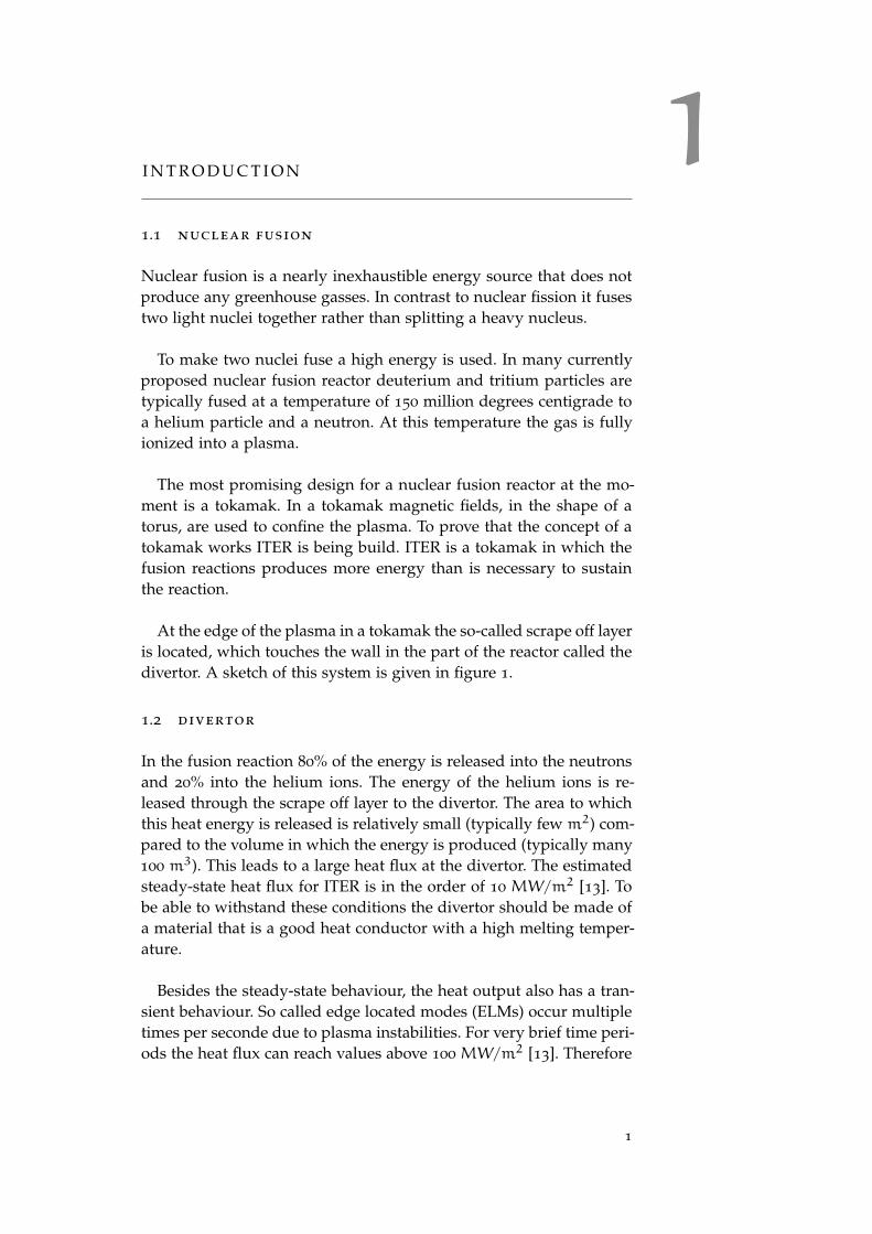
At the edge of the plasma in a tokamak the so-called scrape off layeris located, which touches the wall in the part of the reactor called thedivertor. A sketch of this system is given in figure 1.
1.2 divertor
In the fusion reaction 80% of the energy is released into the neutronsand 20% into the helium ions. The energy of the helium ions is re-leased through the scrape off layer to the divertor. The area to whichthis heat energy is released is relatively small (typically few m2) com-pared to the volume in which the energy is produced (typically many100 m3). This leads to a large heat flux at the divertor. The estimatedsteady-state heat flux for ITER is in the order of 10 MW/m2 [13]. Tobe able to withstand these conditions the divertor should be made ofa material that is a good heat conductor with a high melting temper-ature.
Besides the steady-state behaviour, the heat output also has a tran-sient behaviour. So called edge located modes (ELMs) occur multipletimes per seconde due to plasma instabilities. For very brief time peri-ods the heat flux can reach values above 100 MW/m2 [13]. Therefore
1
2 introduction
Plasma coreFirst wall
Divertor
Scrape off layer
Figure 1: Cross section of a tokamak. The first wall is dashed, the divertoris dash-dotted and the scrape off layer is between the two solidcurves. The tokamak is axial symmetric with the symmetry axison the left side of the image.
the divertor material should have a good thermal shock resistance.
Next to the large heat loads the divertor is also subject to large neu-tron and ion fluxes that constantly bombard the divertor. The neu-trons cause structural changes in the material due to collisions withlattice atoms. This results in swelling of the materials, dislocations ofthe lattice atoms and activation of the material, thereby changing theproperties of the material to undesired properties.
Besides the physical changes that happen to the material due to thebombardment of neutrons, the ions interact with the material, caus-ing swelling and chemical reactions. The plasma exists for a largepart out of hydrogen isotopes (deuterium and tritium) that are highlyreactive radicals. In a nuclear fusion reactor only a small amount oftritium is allowed and because it is radioactive and expensive the di-vertor material should have a low reactivity with tritium.
1.2 divertor 3
This can be summarized in the following properties that a divertormaterial should have [17]:
• High heat conductivity and capacity
• High melting point
• Large thermal shock resistance
• Little degradation of the material properties
• Low activation
• Low tritium retention
• Low erosion yield
• Low plasma pollution of heavy ions
No material has yet been found which has all of these properties.The materials that are currently be considered to be used in ITER aretungsten and carbon fiber composites (CFC). These materials are notideal to use. CFC has the problem that it reacts easily with tritium.Tungsten has the problems that the loss of material into the plasmacan cause a disruption and that it is vulnerable to structural changesdue to neutron radiation and heat cycling.
A proposed mechanism to overcome some of these problems is tocover the divertor surface with a liquid metal. The advantage of aliquid layer is that they have some properties that a solid materialdoes not have, these are[18]:
• No degradation of the material properties
• The material is self healing
• Low recycling
The material does not degraded because the material constantly re-freshes itself with new material. The material is self healing becauseif for whatever reason (ELM, hotspot) the material would evaporate,new material can be brought to the damaged area. If a plasma parti-cle hits the liquid layer it has a high chance to be absorbed into theliquid, this high absorbtion chance is called low recycling. This prin-ciple reduces the plasma pollution as impurities are removed out ofthe reactor, increasing the plasma performance.
Proposed liquids have been gallium, tin and lithium. The advan-tages of tin and gallium over lithium are that they can operate athigher temperatures. The advantages of lithium are: the low atomicmass, it lowers the impurities due to a low recycling rate in the
4 introduction
plasma and it could potentially increase the plasma performance.
The interaction of the liquid metal and the fusion plasma is a majorchallenge in designing a liquid metal divertor. The flow of metals in-side a tokamak induces currents within the liquid metal resulting ina perturbation of the magnetic topology inside the reactor, potentiallyreducing the confinement of the particles. Therefore the flow of thesemetals and the interaction must be well understood.
Concepts of liquid metal divertors has been studied my multipleuniversities. Full liquid wall concepts have been proposed for exam-ple by the University of Los Angeles [6]. In Princeton they have eventested liquid lithium inside a tokamak [8]. None of the publishedconcepts had a system in which they could locally control the liquidmetal flow in the divertor.
A locally controlled liquid metal flow in a divertor would allow foractive control of the divertor performance during its operation. Unde-sired properties of the liquid metal in the divertor could be prevented.An example of this is, if the liquid layer becomes too thin at a certainposition extra material from different locations could be moved tothicken the layer by actively moving that material. Another exampleis to mitigate hotspots, by increasing the flow rate in the location of ahotspot to lower the temperature of the divertor at that location.
The part of the flow which must be controlled in the divertor isthe free surface flow that is exposed to the plasma. The flow can becontrolled by using the strong magnetic fields of a tokamak, in com-bination with a current. To keep the plasma facing part fully liquidthis current could be applied on channels below the surface whichdrive the layer above. In such a system the liquid metal flow can becontrolled by locally controlling the applied current in the divertor.
The concept of such a locally controllable liquid metal flow in adivertor has not yet been published. To be able to control such a flowthe influence of the top layer on the total flow must be known. There-fore the magnetohydrodynamic behaviour of a liquid metal flow in asystem with multiple channels joined on top by a liquid layer mustbe studied.
Besides the concepts using flows of liquid metals in the divertoralternative uses of liquid metals in a divertor have been proposed. Apromising example is the capillary pore system (CPS) [7]. CPS uses aporous structure which sucks up a liquid metal, covering the entirestructure. The main advantages of CPS is that induced currents andmagnetic fields are less of a problem, as the velocity of the liquid

1.2 divertor 5
metal is very low. The main disadvantage of CPS over a liquid metalflow is that the heat cannot be convected out of the divertor. The re-mainder of this report will focus on the concept of using liquid metalflows in divertors instead of other concepts like CPS.
The study that will be performed is more general applicable thanjust on fusion. The magnetic fields and currents will be in the rangethat is achievable with common magnetic fields and moderate cur-rents. In this way the results are also useful for other purposes ofliquid metals whilst still being relevant for liquid metal divertors.
For both experimental and theoretical reasons an axial symmetricgeometry is a convenient geometry to study a liquid metal flow, with-out losing it generality. The experimental reason for this is that exper-iments without begin and end losses can be done, and that no extrapumps or transport systems are needed to move the liquid. From atheoretical view this is interesting because effects of curved channelscan be studied. The symmetry is theoretically also convenient becausethe equations can be solved in cylindrical coordinates, which leads toeasier equations than most other geometries, except straight channels.
The hydrodynamic behaviour of liquid metals has already beenwidely studied. This field of research was started by Hartmann in1937 in straight ducts [12]. Analytical solutions have been found forthe velocity fields in multiple geometries (e.g. flow between parallelplates, strait ducts, etc.). During the years this research has been ex-panded towards other geometries. For experimental reasons an annu-lar set-up is often studied [2]. Most of this research has been focussedon closed channels with either radial magnetic fields or an axial mag-netic field [14]. The liquid was forced by applying, perpendicular tothe magnetic field, an electric field.
No study has been published in a geometry that would be relevantfor the concept of a locally controlled liquid metal divertor. Such ageometry would consist of multiple electromagnetically driven chan-
Figure 2: Geometry of a set-up with multiple concentric annular channels.On the bottom of the container the channels are drawn. Overthese channels a potential difference can be applied. In combina-tion with a magnetic field this current exerts a force on the liquidinside the container.
6 introduction
nels, which drive a bulk layer on top. As explained it is most conve-nient to do this in an annular set-up. This geometry is depicted infigure 2, in here the magnetic field is in vertical direction, the currentin radial direction and the resulting flow in azimuthal direction.
1.3 goal
To be able to design a locally controllable liquid metal divertor theamount of fluid that is be transported by the divertor using the con-trol parameters (magnetic field, electric current) must be known. Thisdependence of amount of fluid that is driven by a magnetic field andcurrent will be studied in this report. To be able to compare the re-sults of both an experiment and a theoretical analysis the velocity fluxat the surface will be used as a reference parameter. To use a liquidmetal flow in a divertor the influence of the top layer on response ofthe flow to the control parameters must be know, especially in whatway the velocity flux at the surface scales with these parameters. Tostudy this the following research question has been formulated:
What is the influence of a top layer, driven by a system of concentric annu-lar channels, on the the scaling of the velocity flux at the surface of a liquidmetal with the control parameter, the magnetic field and the electric current.
To be able to compare theoretical predictions with experimental re-sults a secondary question must be answered:
How does the scaling of the velocity flux at the surface change if the mag-netic field is is not perfectly parallel and perpendicular to the surface
To answer this question a simulation will be made with two dif-ferent magnetic configurations which can simulate: a magnetohydro-dynamic flow in a system of annular channels for different magneticfield and currents in the relevant domain. To limit the scope of boththe research question and the goal the relevant domain will be lami-nar flows, because in this range the relevant scaling behaviour is ex-pected to happen. The forcing in the simulations is due to the Lorentzforce from a magnetic field that has mainly components in verticaldirection and an applied potential over the channels. From this simu-lation the velocity flux at the surface will be obtained.
1.4 methods
The work will be mainly be based on numerical simulations. To sup-port the simulations the scaling behaviour is also analyzed from atheoretical point of view. To be able to compare the simulations toexperimental data a pilot experiment has been designed. The set-up
1.5 outline 7
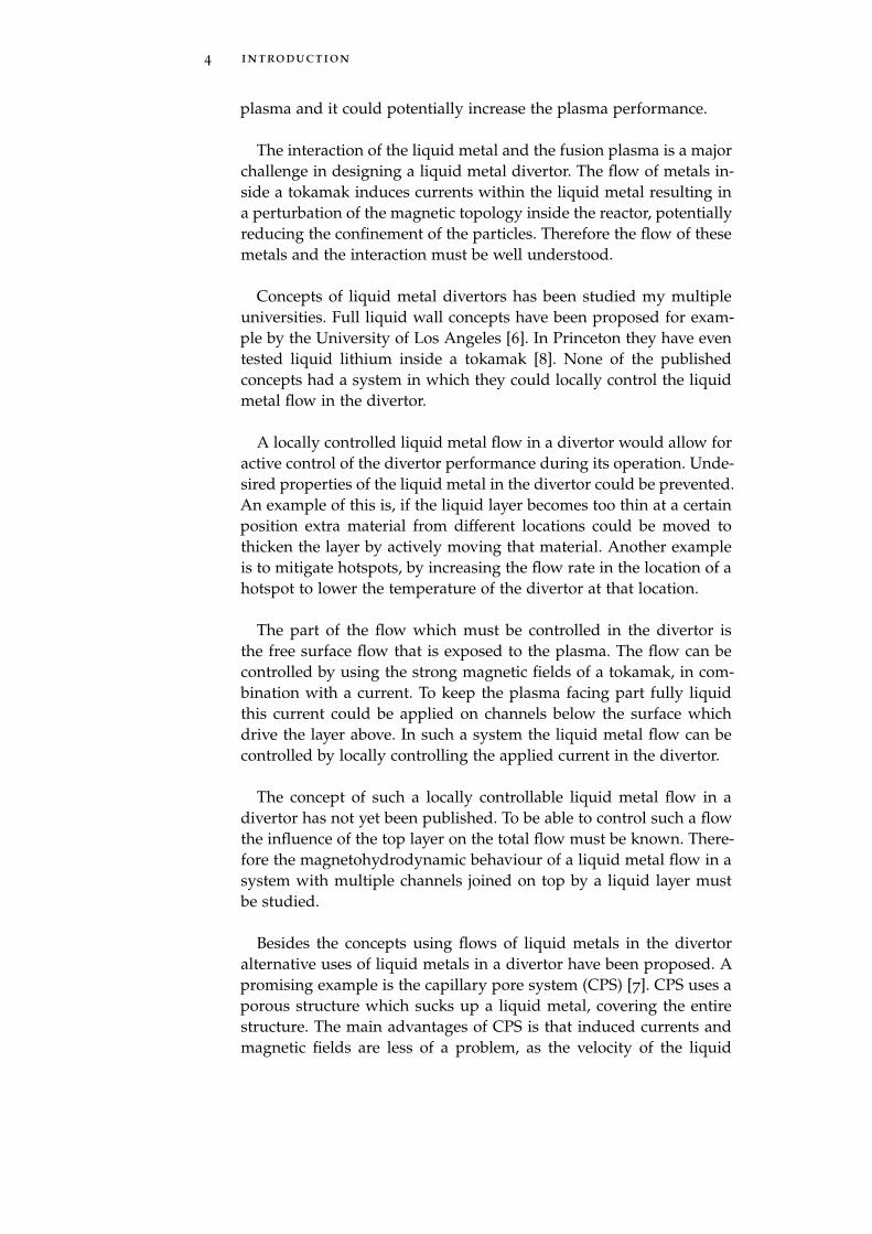
symmetry axis
Liquid metal
PVC container
magnets
electrodes
Figure 3: Set-up of annular channels joined on top by a bath. This geometryis used in a pilot experiment to study the behaviour of a liquidmetal flow, the same dimensions are used in the simulations.
and experiments are described in the report of Koelman [15]. But theexperimental data does not yet offer conclusive data to underpin thesimulations. Many of geometrical choices in the simulation have beenbased on this experiment, like the channel width, depth and inner ra-dius, position and strength of the bar magnets, etc. The geometry ofthe experiment is depicted in figure 3. The material that was used inthe experiment was galinstan, therefore its properties are used in thesimulation.
The simulation software that is used is COMSOL version 4.3a. COM-SOL is a widely used simulation package that can solve differentialequation using a finite element method. Dedicated MHD-codes alsoexist, but due to the availability and adaptability of COMSOL (it eas-ily be extended to solve combined physical phenomena) it was chosento develop a simulation of a liquid metal flow in COMSOL.
To check whether the simulation is valid and correct in the rangewhere scaling is studied the simulations are benchmarked againstknown solutions and compared to other numerical simulations. Us-ing the benchmarked simulation, studies of the relevant geometrieswill be made. From these simulations the scaling behaviour at thesurface of the liquid metal flow is obtained.
1.5 outline
The theoretical analysis is explained in chapter 2 by reviewing themagnetohydrodynamic theory. From this theory simple qualitativescaling laws are derived. The numerical framework that is used inCOMSOL and its relation to the theory is described in chapter 3. Thebenchmarks are explained and done in chapter 4. In chapter 5 the

8 introduction
results from the simulation will be explained and analyzed to givequantitative values for the scaling behaviour. From this work the con-clusion, discussion and future directions will be given.
2M A G N E T O H Y D R O D Y N A M I C S
In this chapter a theoretical analysis of liquid metal flows is made.First the magnetohydrodynamic (MHD) equations are presented, alongwith some other relevant equations. Buckingham’s Π theorem is usedto find the relevant parameters of the equations. After that the scalingof the velocity flux at the surface with these parameter is studied.
2.1 the magnetohydrodynamic equations
The MHD theory describes the motion of a conducting fluid and itsinteraction with magnetic and electric fields. The MHD equations con-sist of Maxwell’s laws for electromagnetism, the Navier-Stokes equa-tion for hydrodynamics and the conservation of mass. The equationsare:
Maxwell’s equations:
∇ · ~E =ρEε0
(1)
∇ · ~B = 0 (2)
∇× ~E = −∂~B
∂t(3)
∇× ~B = µ0~J+ µ0ε0∂~E
∂t(4)
Navier-Stokes equation:
ρ
(∂~v
∂t+~v · ∇~v
)= −∇p+ µ∇2~v+ ρE~E+~J× ~B+~Fother (5)
Conservation of mass:dρ
dt+ ρ∇ ·~v = 0 (6)
The definition of the terms are:
~E Electric fieldρE Electric charge densityε0 Electric permittivity of vacuum~B Magnetic fieldµ0 Magnetic permeability of vacuum~J Currentρ Density~v Velocityµ Dynamic viscosity
9
10 magnetohydrodynamics
Maxwell’s equations in combination with the Navier-Stokes equa-tion and the conservation of mass describe: the electric field, the mag-netic fields and the flow of a liquid metal. Two other useful electro-magnetic relations are the Lorentz force and Ohm’s law. The Lorentzforce gives the relation between the electromagnetic fields and theforce exerted on a charged body (this equation was already used in5):
~F = ρ~E+~J× ~B (7)
The current is induced by two mechanisms. The first one is the ap-plied electric field the second mechanism is the motion through anapplied magnetic field of the fluid. This combination leads to Ohm’sLaw:
~J = σ(~E+~v× ~B
)(8)
Solving the MHD equations for the appropriate boundary condi-tions yields the electric field, the magnetic fields and the velocity fieldof the flow. These differential equations have in general no analyticalsolution, only in some special cases. Therefore numerical methodsare needed to solve these equations. The numerical framework that isused to solve these equations in the simulations is described in chap-ter 3.
In these equations no induced magnetic fields have been assumed.This assumption is valid because the magnetic Reynolds number issmall for typical conditions encountered in our applications. The mag-netic Reynolds number is a dimensionless number that gives an esti-mate of the effects of the magnetic advection to the magnetic diffusion(Rm = µσLv0). When this number is small it can be assumed that theinduced magnetic field are small enough that they can be neglected.
2.2 buckingham’s Π theorem
As can be seen in the Navier-Stokes equation 5 the flow responds tothe forcing of the flow. This forcing can either be internal or external.In the simulations an internal forcing by means of an applied currentand magnetic field is used. To study the scaling behaviour of the flowon the forcing Buckingham’s Π theorem is used [3]. Buckingham’s Πtheorem allows to create a complete set of independent dimension-less variables of a problem.
In the simulations the velocity flux at the surface is the output pa-rameter of interest. There are three reasons for that. The first one isthat if the velocity flux at the surface is important in the concept ofliquid metal divertors in tokamaks. The velocity flux at the surfacesdetermines the amount of heat the flow can absorb at the surface. The
2.2 buckingham’s Π theorem 11
second reason is for experimental convenience, in an experiment it isrelatively easy to determine the velocity flux at the surface, opposedto determining the total Velocity flux rate. The third reason is thatone expects the velocity flux to change with a changing forcing, asthe velocity is expected to change.
The derivation of the results in Buckingham’s Π theorem can befound in the appendix . The results are presented in this section. Thevelocity flux at the surface is a function of:
Qs = f (v, ρ,µ,a, I,B,σ,µm) (9)
The definitions of the new terms are:
Q Velocity flux at the surfaceI Applied current on the channelsσ Electrical conductivitya Width of the channels
There are nine variables and four physical quantities (length, time,mass and current). According to Buckingham’s Π theorem there are(9 - 4) = 5 independent dimensionless numbers. These numbers canbe obtained from this function:
Π = Qa1s va2ρa3µa4aa5Ia6Ba7σa8µa9m (10)
As repeating variables µ,a,σ,µm are chosen. These are chosen be-cause they allow to compare the different geometries. This results inthe following dimensionless numbers:
Π1 =Qsσµm
aDimensionless velocity flux at the surface (11)
Π2 = vaσµm Dimensionless velocity (12)
Π3 =ρ
µσµmDimensionless density (13)
Π4 = Iµm
√σ
µDimensionless current (14)
Π5 = Ba
√σ
µDimensionless magnetic field (15)
The last dimensionless number (Π5) is in the literature known as theHartmann number (Ha).
As stated before in the simulations the parameter of interest is thevelocity flux at the surface. The dimensionless variant of this is the’dimensionless velocity flux’ Π1. The typical velocity Π2 could alsohave been used as a output parameter of the system, but this will notbe done. The reason is that the velocity flux at the surface is moreinteresting to study for experimental and divertor reasons. The di-mensionless number Π3 is a parameter of the system and can not be
12 magnetohydrodynamics
changed. The dimensionless current Π4 is one of the variables thatcan be changed. It can be changed by the applied voltage over thechannels. A larger value of Π4 will result in a larger forcing of thefluid. Similarly the Hartmann number Π5 influences the flow.
From Buckingham’s Π theorem it can be concluded that the dimen-sionless current Π4 and the Hartmann number Ha influence the flow,which can be characterized by both the dimensionless velocity fluxat the surface Π1 and dimensionless velocity Π2. For the simulationthe scaling behaviour of the velocity flux at the surface on both thecurrent and magnetic field will be studied. For better readability thedimensionless current Π4 will be assigned the variable ID.
2.3 scaling of the velocity flux at the surface
To study the scaling behaviour of such a flow it would be very conve-nient to have an analytic solution. But no analytic solution is knownfor open annular channels. Solutions do exist for straight channelflows. Since that these analytic solutions offer a very good insight inthe scaling behaviour they will be presented here first. After that thechanges for an open annular channels will be given.
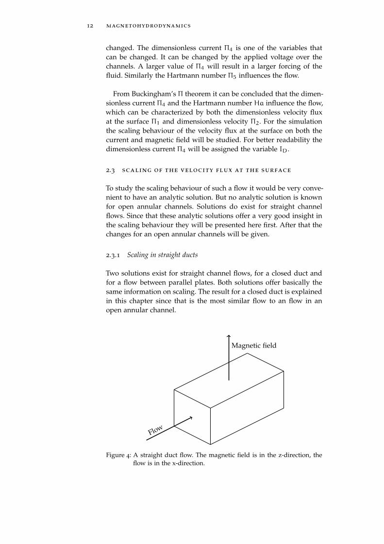
2.3.1 Scaling in straight ducts
Two solutions exist for straight channel flows, for a closed duct andfor a flow between parallel plates. Both solutions offer basically thesame information on scaling. The result for a closed duct is explainedin this chapter since that is the most similar flow to an flow in anopen annular channel.
Flow
Magnetic field
Figure 4: A straight duct flow. The magnetic field is in the z-direction, theflow is in the x-direction.

2.3 scaling of the velocity flux at the surface 13
0 0.2 0.4 0.6 0.8 10
0.2
0.4
0.6
0.8
1
Position from center (normalized units)
Nor
mal
ized
velo
city
Ha = 0Ha = 1Ha = 10Ha = 100
Figure 5: Flow profiles for different Hartmann numbers in a straight duct,the lines for Ha = 0 and Ha = 1 barely differ.
A flow of a liquid metal under electromagnetic forcing is called aHartmann flow. The closed duct flow is analyzed to be able to under-stand the physical phenomena that happen in a Hartmann flow. Asketch of the system is given in figure 4. The flow is driven by a con-stant pressure gradient. Such a gradient can be achieved by applyingan electric field in the y-direction. This yields a constant current inthe same direction. The solution found by Shercliff [16] of the flow is:
v =
∞∑i=1,3,5
vi(y)cos(λix) (16)
with:
λi =iπ
2a
ki = 2sin(λia)
λia
pi1,2 =1
2
(Ha∓
√Ha2 + 4λ2i
)αi1,2 = sinh
(pi1,2
)fi(y) = αi2cosh (pi1y) −αi1cosh (pi2y)
vi(y) =ki
λ2i
(1−
fi(y)
fi(1)
)In figure 5 the profile of the flow is plotted for several different Hart-mann numbers.
As can be seen in figure 5 the velocity profile at higher Hartmannnumber tend to level out. The profile gets flatter because when aconductor moves through a magnetic field a current is induced. This
14 magnetohydrodynamics
10−2 10−1 100 10110−2
10−1
100
Hartmann number
Nor
mal
ized
volu
met
ric
rate
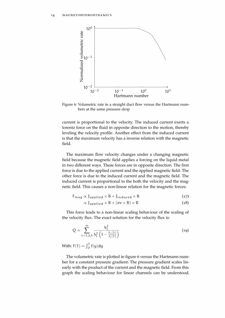
Figure 6: Volumetric rate in a straight duct flow versus the Hartmann num-bers at the same pressure drop
current is proportional to the velocity. The induced current exerts alorentz force on the fluid in opposite direction to the motion, therebyleveling the velocity profile. Another effect from the induced currentis that the maximum velocity has a inverse relation with the magneticfield.
The maximum flow velocity changes under a changing magneticfield because the magnetic field applies a forcing on the liquid metalin two different ways. These forces are in opposite direction. The firstforce is due to the applied current and the applied magnetic field. Theother force is due to the induced current and the magnetic field. Theinduced current is proportional to the both the velocity and the mag-netic field. This causes a non-linear relation for the magnetic forces:
Fmag ∝ Japplied ×B+ Jinduced ×B (17)
∝ Japplied ×B+ (σv×B)×B (18)
This force leads to a non-linear scaling behaviour of the scaling ofthe velocity flux. The exact solution for the velocity flux is:
Q =
∞∑i=1,3,5
k2i
λ2i
(1−
Fi(1)fi(1)
) (19)
With: F(1) =∫10 f(y)dy
The volumetric rate is plotted in figure 6 versus the Hartmann num-ber for a constant pressure gradient. The pressure gradient scales lin-early with the product of the current and the magnetic field. From thisgraph the scaling behaviour for linear channels can be understood.
2.3 scaling of the velocity flux at the surface 15
As can be seen from the graph the volumetric scales linearly with theHartmann number until a certain critical value near one. After thisthreshold the velocity flux drops for higher Hartmann number. Thevelocity flux at the surface is expected to scale in very similar way tothe volumetric rate in a channel.
From graph 6 it can also be concluded that the velocity flux scaleslinearly with the current. This is because the pressure gradient scaleslinearly with the product of the magnetic field and current and thefact that this graph is valid for all pressure gradients.
2.3.2 Scaling in an open annular channels
The free surface at top of the flow leads to a different boundary con-dition for the flow. The top boundary now has a stress free boundarycondition instead of a no-slip condition. Therefore the flow can havea velocity at that boundary.
When a current is applied to an annular channel the current den-sity is not constant anymore, since the current goes through a largerarea on the outside of the channel than on the inside. This yields a1/r dependence of the current density.
Due to the fact that an annular channel is curved the flow willbehave differently. What changes happen and why will be explainedby looking at the Navier-Stokes equation in cylinder coordinates.
r :
ρ
(∂ur
∂t+ ur
∂ur
∂r+uφ
r
∂ur
∂φ+ uz
∂ur
∂z−u2φ
r
)= −
∂p
∂r+
µ
(1
r
∂
∂r
(r∂ur
∂r
)+1
r2∂2ur
∂φ2+∂2ur
∂z2−ur
r2−2
r2∂uφ
∂φ
)+ Fr
(20)
φ :
ρ
(∂uφ
∂t+ ur
∂uφ
∂r+uφ
r
∂uφ
∂φ+ uz
∂uφ
∂z+uruφ
r
)= −
1
r
∂p
∂φ+
µ
(1
r
∂
∂r
(r∂uφ
∂r
)+1
r2∂2uφ
∂φ2+∂2uφ
∂z2+2
r2∂ur
∂φ−uφ
r2
)+ Fφ
(21)
z :
ρ
(∂uz
∂t+ ur
∂uz
∂r+uφ
r
∂uz
∂φ+ uz
∂uφ
∂z
)= −
∂p
∂z+
µ
(1
r
∂
∂r
(r∂uz
∂r
)+1
r2∂2uz
∂φ2+∂2uz
∂z2
)+ Fz
(22)
16 magnetohydrodynamics
In the equations a couple of extra terms become apparent, all of theseterms have either a 1/r or 1/r2 dependency. The coupling of theseterms with the radius of the channel induces a secondary flow.
The secondary flow moves outwards on the top of the flow andthen moves downward along the outer wall to move inwards overthe bottom. The most popular explanation was given by Einstein in1926 [5]. He used it to explain the erosion of rivers banks and themovement of tea leafs in a cup whilst stirring it.
The secondary motion is induced by the centripetal force needed bythe fluid to follow the curved annular channel. A pressure gradientyields this force. The flow has a smaller velocity near the bottom andthe sides of the channel. Therefore the centrifugal force is smallerthere. The pressure gradient however remains intact. The pressuregradient at the bottom is thus larger than the centrifugal force induc-ing an inward motion of the liquid at the bottom. This effect createsa circular secondary flow in annular channel.
A part of the energy of the primary flow goes to the secondary flow.This causes a less efficient forcing of the system then a straight chan-nel, i.e. more force is needed to keep the flow moving with the samevelocity. The secondary flow becomes important when the velocity ishigh enough. This means that at high forcing (i.e. large J× B) thereis less efficient forcing than at low forcing. This leads to sub-linearscaling at large values of J×B.
The magnetic field influences the flow in much the same way inannular channels as it does in straight ducts. Currents are inducedby the magnetic field. These currents balance the applied currents inthe center of the flow, thereby leveling the velocity profile. The ve-locity profile is not leveled to a flat pattern as in a straight channelbut to a 1/r profile. This is because of the shape of the current density.
The phenomena explained in this section lead to a poorer efficiencyof the forcing of the velocity flux at the surface. Therefore the scalingis influenced by this.
From these two different types of scaling it is expected that thereare three regimes of different scaling of the velocity flux at the surface.The first regime is for small dimensionless currents and Hartmannnumbers. In this regime linear scaling behaviour is expected, sincethe flow reacts linear to the forcing in this regime. This regime willbe called the linear regime.
2.3 scaling of the velocity flux at the surface 17
Linear scaling
Magnetic braking
Curvature
Hartman number
Dim
ensi
onle
sscu
rren
t
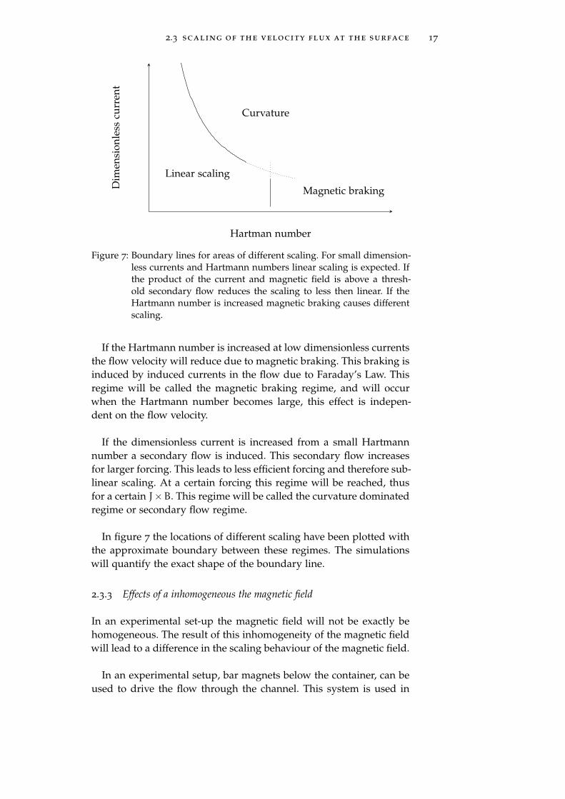
Figure 7: Boundary lines for areas of different scaling. For small dimension-less currents and Hartmann numbers linear scaling is expected. Ifthe product of the current and magnetic field is above a thresh-old secondary flow reduces the scaling to less then linear. If theHartmann number is increased magnetic braking causes differentscaling.
If the Hartmann number is increased at low dimensionless currentsthe flow velocity will reduce due to magnetic braking. This braking isinduced by induced currents in the flow due to Faraday’s Law. Thisregime will be called the magnetic braking regime, and will occurwhen the Hartmann number becomes large, this effect is indepen-dent on the flow velocity.
If the dimensionless current is increased from a small Hartmannnumber a secondary flow is induced. This secondary flow increasesfor larger forcing. This leads to less efficient forcing and therefore sub-linear scaling. At a certain forcing this regime will be reached, thusfor a certain J×B. This regime will be called the curvature dominatedregime or secondary flow regime.
In figure 7 the locations of different scaling have been plotted withthe approximate boundary between these regimes. The simulationswill quantify the exact shape of the boundary line.
2.3.3 Effects of a inhomogeneous the magnetic field
In an experimental set-up the magnetic field will not be exactly behomogeneous. The result of this inhomogeneity of the magnetic fieldwill lead to a difference in the scaling behaviour of the magnetic field.
In an experimental setup, bar magnets below the container, can beused to drive the flow through the channel. This system is used in

18 magnetohydrodynamics
the experiments and is depicted in figure 3. In such a set-up the mag-netic field is strongest at the bottom of the channel. This is where thevelocity gradient is the highest. Because of the higher magnetic fieldthe gradient will be reduced, resulting in a lower maximum velocityat the surface of the flow.
The secondary flows will also be influenced by the inhomogeneousmagnetic fields, as they move through a constantly changing mag-netic field. This will result in a different velocity profile and might in-fluence the shape and location of the boundary between the regimesof different scaling.
3N U M E R I C A L F R A M E W O R K
The MHD equations that were presented in the last chapter will besolved numerically, this will be done using a program called COM-SOL multiphysics. COMSOL is a simulation package that solves dif-ferential equations using a finite element method.
This chapter starts with an introduction of the parts (modules) thatare used in COMSOL. This is followed by the implementation of themagnetohydrodynamic equations in COMSOL. After that the bound-ary conditions for MHD-flows are explained. In the last section thephenomena with the smallest spatial dimension will be described andquantified. From this the minimum size of the mesh elements will bedetermined to resolve these phenomena.
3.1 comsol modules
COMSOL uses modules to simulate different physical principles ormathematics. These modules can be combined to simulate multiplephysical phenomena. To simulate a Hartmann flow the followingmodules are used:
• Laminar flow (spf)
• Poisson’s equation (poeq)
• Magnetic fields (mf)
The ’Laminar flow’ module is used to solve the Navier-Stokes equa-tion. This module allows to simulate laminar flow.
The ’Poisson’s equation’ module calculates the electric fields andcurrents. Both the applied and induced fields are calculated usingthis module.
The magnetic fields are calculated using the ’magnetic fields’ mod-ule. The magnetic field can be decoupled from the currents since themagnetic Reynolds number is small, see section 2.1. Therefore no in-duced magnetic field needs to be calculated.
Two different magnetic fields are used in the simulation. The first isa constant vertical magnetic field. This magnetic field is not simulated,the strength is directly used in the calculation of the Lorentz forcein the Navier-Stokes equation and Poisson’s equation. The second
19
20 numerical framework
magnetic field is a more realistic field. This field has both verticaland radial components. This magnetic field is calculated using themagnetic fields module in COMSOL.
3.2 mathematical framework
3.2.1 Poisson’s equation
The electric potential is calculated using Poisson’s equation with theappropriate boundary conditions and sources terms. From Poisson’sequation the electric current is obtained. In electrostatics Poisson’sequation is defined as:
∇2V = −ρ
ε0(23)
Poisson’s equation has the following definition in COMSOL:
∇ · (−c∇V) = f (24)
This can be rewritten from Ohm’s law 8 in the stationary state to:
∇2V = ∇ · (v×B) (25)
A special note on this must be taken in COMSOL for cases withcylindrical coordinates. Which is relevant for doing simulations withan axial symmetry. Laplace’s operator in COMSOL is defined as:
∇2COMSOLV =∂2V
∂r2+∂2V
∂φ2+∂2V
∂z2(26)
Whereas the Laplacian in cylinder coordinates is defined as:
∇2V =1
r
∂
∂r
(r∂V
∂r
)+1
r2∂2V
∂φ2+∂2V
∂z2(27)
=1
r
∂V
∂r+∂2V
∂r2+1
r2∂2V
∂φ2+∂2V
∂z2
Therefore the following correction factor is need to translate fromCOMSOL’s Poisson’s equation to the normal one:
∇2V = ∇2COMSOLV +1
r
∂V
∂r(28)
This system can be solved for the appropriate boundary conditions.
3.2.2 Boundary conditions for Poisson’s equation
To drive a current, a potential is applied over the channel. This caneasily be applied as a boundary condition of Poisson’s equation. Theother boundaries of the system are electric insulators. This means that
3.2 mathematical framework 21
no current flow through the wall, i.e. J · n = 0. Using Ohm’s law theinsulating boundary conditions can be obtained:
J · n = σ (E+ v×B) · n = 0 (29)
If a purely vertical magnetic field is used B = B0ez the v× B termdrops out since through either (v×B)z = vxBy−vyBx = 0 or (v×B)z =vrBφ − vφBr = 0, thus the boundary condition becomes:
E · n = 0 (30)
This translates in a boundary condition for the potential as:
∂V
∂z= 0 (31)
If more realistic magnetic fields are used, that is a vertical fieldwith radial components. The boundary conditions become in eithercartesian or cylinder coordinates for the free surface:
Cartesian:∂V
∂z= vxBy − vyBx (32)
Cylinder:∂V
∂z= vrBφ − vφBr (33)
The boundary conditions in combination with equation 25 given theelectric potential in the channels.
3.2.3 Current calculation
The potential is coupled to the Navier-Stokes module through theLorentz force on the fluid. The Lorentz force 7 uses the current anda magnetic field. The current is calculated from the potential usingOhm’s law 8:
J = σ (E+ v×B) (34)
= σ (−∇V + v×B) (35)
From this current the Lorentz force can be calculated:
F = J×B (36)
The Lorentz force is used as a volume force in the laminar flow mod-ule of COMSOL. The laminar flow module and Poisson’s equationsmodule can together be solved for the appropriate boundary condi-tions and magnetic field to obtain the flow a liquid metal in COM-SOL.
22 numerical framework
3.3 meshing
The mesh size determines the precision to which a solution can befound. The mesh size must be optimized to allow for fast calcula-tions, a coarser mesh is faster calculated than a finer mesh. But acoarse mesh might not always be able to resolve all physical phenom-ena.
The mesh should be the finest in the places with the highest gradi-ents, which is at the walls of the system. At the walls the Hartmannlayer and side layer are located. The Hartmann layer is located atbottom of a channel and its size is given by:
δH =
õ
B2σ(37)
The side layers are located at the vertical walls, where electrodes arethat drive the flow, their thickness is given by:
δS =
√L
B·√µ
σ(38)
Inside these layers multiple points are needed to correctly calculatethe flow. In the simulations typically at least 10 points were usedin the Hartmann layer and side layer. In the core of the flow largerelement sizes are allowed. Other properties of the flow or solver canmake smaller element sizes necessary, but in general these numbersyield a good approximation for the minimal element size.
4B E N C H M A R K I N G
In the last chapter a numerical framework has been introduced tocalculate a Hartmann flow. In this chapter the framework will be ver-ified. In total three different benchmarks will be used to validate allparts of the simulation.
The first benchmark is a flow between to infinitely long cylinders.The fluid will be driven by a potential difference between the cylin-ders. By comparing the analytical solution of this flow with the resultsfrom the simulation it can be checked whether the simulation is cor-rectly implemented in cylindrical coordinates.
The second benchmark is the flow in an infinitely long straight duct.The analytical solution of this flow will be compared to a simulationof a flow in an annular channel with a small aspect ratio. Both so-lutions are expected to have a similar solution because of the smallaspect ratio of the annular channel. With this simulation the correctimplementation of the boundary conditions and the response to themagnetic field can be validated.
The last benchmark is also a flow in an annular channel, but nowwith a large aspect ratio. This large aspect ratio allows for a validationof the effect of the curvature i.e. the secondary flow. This benchmarkwill be done by comparing the solution of the simulation with a sim-ulation published by Vantieghem and Knaepen.
Therefore all relevant phenomena of a laminar MHD-flow in anannular channel with a forcing by a radial current and a vertical mag-netic field can be validated using these benchmarks.
The comparisons will be made in the relevant range for the simu-lations. This range is for the Hartmann number from zero (hydrody-namic flow) to a hundred (strong magnetic braking). This covers therange in which changes are expected to happen. The electric potentialis chosen at a value that the flow is laminar. The current in the com-parison with the model of Vantieghem and Knaepen will be chosento match their Reynolds numbers.
23
24 benchmarking
4.1 flow between two cylinders duct
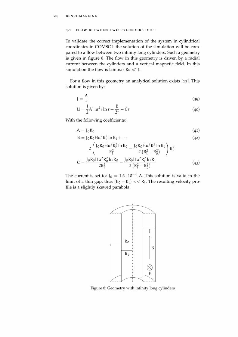
To validate the correct implementation of the system in cylindricalcoordinates in COMSOL the solution of the simulation will be com-pared to a flow between two infinity long cylinders. Such a geometryis given in figure 8. The flow in this geometry is driven by a radialcurrent between the cylinders and a vertical magnetic field. In thissimulation the flow is laminar Re� 1.
For a flow in this geometry an analytical solution exists [11]. Thissolution is given by:
J =A
r(39)
U =1
2AHa2r ln r−
B
2r+Cr (40)
With the following coefficients:
A = J0R0 (41)
B = J0R0Ha2R2i lnRi + · · · (42)
2
(J0R0Ha
2R20 lnR0R2i
−J0R0Ha
2R2i lnRi2(R2i − R
20
) )R2i
C =J0R0Ha
2R20 lnR02R2i
−J0R0Ha
2R2i lnRi2(R2i − R
20
) (43)
The current is set to: J0 = 1.6 · 10−4 A. This solution is valid in thelimit of a thin gap, thus (R0 − Ri) << Ri. The resulting velocity pro-file is a slightly skewed parabola.
Ri
R0
J
B
F
Figure 8: Geometry with infinity long cylinders
4.1 flow between two cylinders duct 25
0 0.2 0.4 0.6 0.8 10
0.2
0.4
0.6
0.8
1
r−RiR0−Ri
Nor
mal
ized
velo
city
(a) Hartmann number = 0.1
0 0.2 0.4 0.6 0.8 10
0.2
0.4
0.6
0.8
1
r−RiR0−Ri
Nor
mal
ized
velo
city
(b) Hartmann number = 1
0 0.2 0.4 0.6 0.8 10
0.2
0.4
0.6
0.8
1
r−RiR0−Ri
Nor
mal
ized
velo
city
(c) Hartmann number = 10
0 0.2 0.4 0.6 0.8 10
0.2
0.4
0.6
0.8
1
r−RiR0−Ri
Nor
mal
ized
velo
city
(d) Hartmann number = 100
Simulations Theory
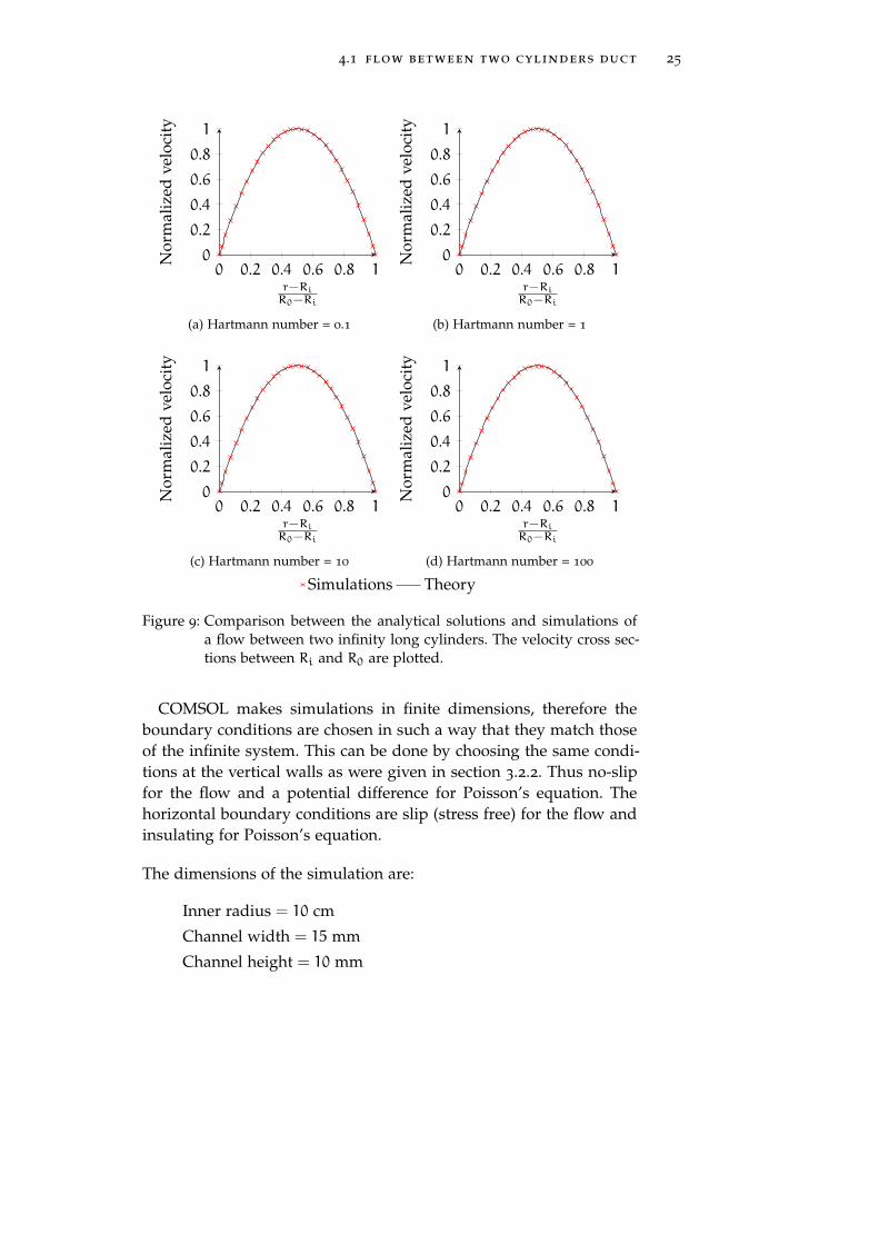
Figure 9: Comparison between the analytical solutions and simulations ofa flow between two infinity long cylinders. The velocity cross sec-tions between Ri and R0 are plotted.
COMSOL makes simulations in finite dimensions, therefore theboundary conditions are chosen in such a way that they match thoseof the infinite system. This can be done by choosing the same condi-tions at the vertical walls as were given in section 3.2.2. Thus no-slipfor the flow and a potential difference for Poisson’s equation. Thehorizontal boundary conditions are slip (stress free) for the flow andinsulating for Poisson’s equation.
The dimensions of the simulation are:
Inner radius = 10 cm
Channel width = 15 mm
Channel height = 10 mm
26 benchmarking
0 0.2 0.4 0.6 0.8 110−5
10−4
10−3
10−2
r−RiR0−Ri
Diff
eren
ce
(a) Hartmann number = 0.1
0 0.2 0.4 0.6 0.8 110−5
10−4
10−3
10−2
r−RiR0−Ri
Diff
eren
ce
(b) Hartmann number = 1
0 0.2 0.4 0.6 0.8 110−5
10−4
10−3
10−2
r−RiR0−Ri
Diff
eren
ce
(c) Hartmann number = 10
0 0.2 0.4 0.6 0.8 110−5
10−4
10−3
10−2
r−RiR0−Ri
Diff
eren
ce
(d) Hartmann number = 100
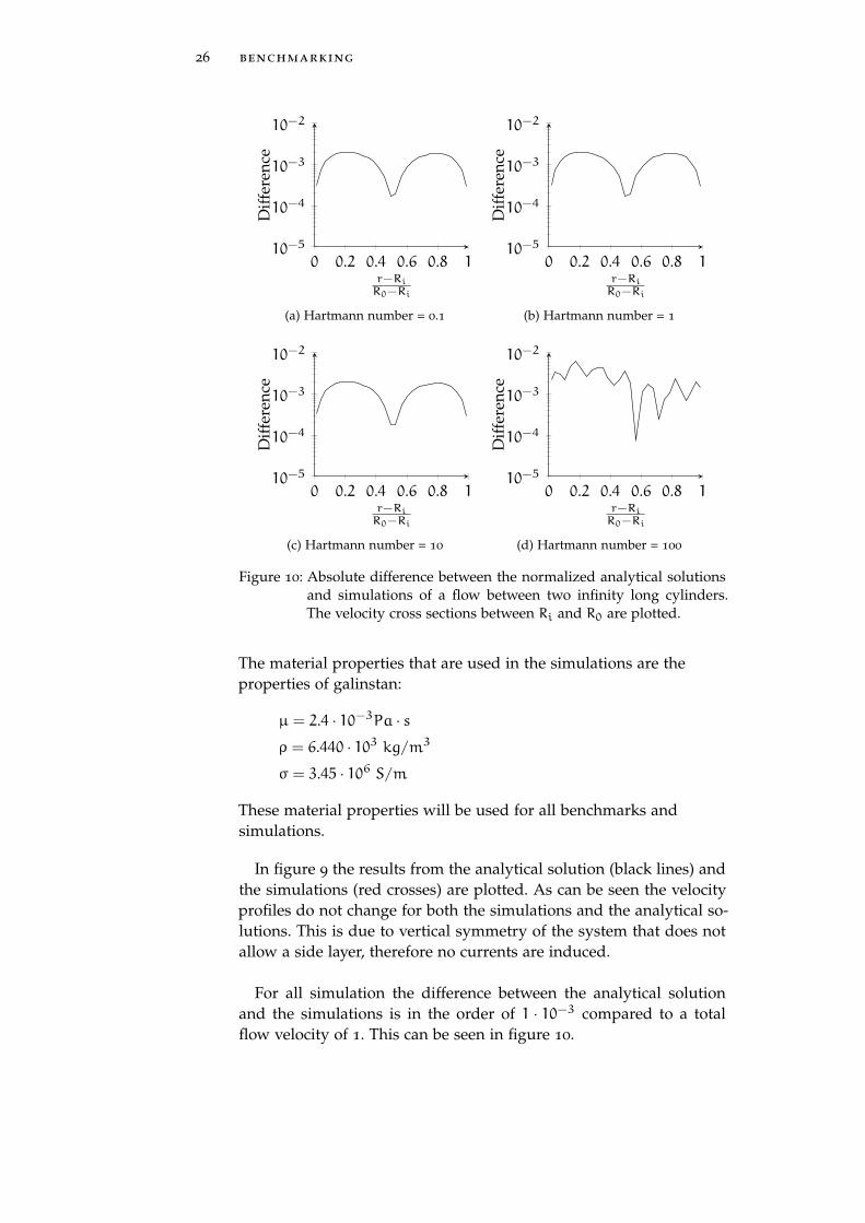
Figure 10: Absolute difference between the normalized analytical solutionsand simulations of a flow between two infinity long cylinders.The velocity cross sections between Ri and R0 are plotted.
The material properties that are used in the simulations are theproperties of galinstan:
µ = 2.4 · 10−3Pa · sρ = 6.440 · 103 kg/m3
σ = 3.45 · 106 S/m
These material properties will be used for all benchmarks andsimulations.
In figure 9 the results from the analytical solution (black lines) andthe simulations (red crosses) are plotted. As can be seen the velocityprofiles do not change for both the simulations and the analytical so-lutions. This is due to vertical symmetry of the system that does notallow a side layer, therefore no currents are induced.
For all simulation the difference between the analytical solutionand the simulations is in the order of 1 · 10−3 compared to a totalflow velocity of 1. This can be seen in figure 10.
4.2 straight square duct flow 27
From the solutions of the analytical solution and the simulation canbe concluded that they closely match. This means that numericallyframework is complete enough to simulate a liquid metal flow in anaxial symmetric system with these boundary conditions. Also it canbe concluded that the numerical frame work is correctly implementedin COMSOL.
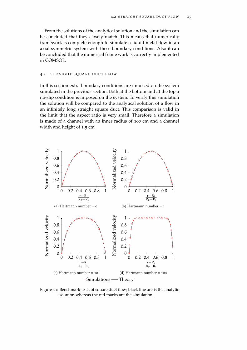
4.2 straight square duct flow
In this section extra boundary conditions are imposed on the systemsimulated in the previous section. Both at the bottom and at the top ano-slip condition is imposed on the system. To verify this simulationthe solution will be compared to the analytical solution of a flow inan infinitely long straight square duct. This comparison is valid inthe limit that the aspect ratio is very small. Therefore a simulationis made of a channel with an inner radius of 100 cm and a channelwidth and height of 1.5 cm.
0 0.2 0.4 0.6 0.8 10
0.2
0.4
0.6
0.8
1
r−RiR0−Ri
Nor
mal
ized
velo
city
(a) Hartmann number = 0
0 0.2 0.4 0.6 0.8 10
0.2
0.4
0.6
0.8
1
r−RiR0−Ri
Nor
mal
ized
velo
city
(b) Hartmann number = 1
0 0.2 0.4 0.6 0.8 10
0.2
0.4
0.6
0.8
1
r−RiR0−Ri
Nor
mal
ized
velo
city
(c) Hartmann number = 10
0 0.2 0.4 0.6 0.8 10
0.2
0.4
0.6
0.8
1
r−RiR0−Ri
Nor
mal
ized
velo
city
(d) Hartmann number = 100
Simulations Theory
Figure 11: Benchmark tests of square duct flow; black line are is the analyticsolution whereas the red marks are the simulation.
28 benchmarking
0 0.2 0.4 0.6 0.8 110−5
10−4
10−3
10−2
r−RiR0−Ri
Diff
eren
ce
(a) Hartmann number = 0
0 0.2 0.4 0.6 0.8 110−5
10−4
10−3
10−2
r−RiR0−Ri
Diff
eren
ce
(b) Hartmann number = 1
0 0.2 0.4 0.6 0.8 110−5
10−4
10−3
10−2
r−RiR0−Ri
Diff
eren
ce
(c) Hartmann number = 10
0 0.2 0.4 0.6 0.8 110−5
10−4
10−3
10−2
r−RiR0−Ri
Diff
eren
ce
(d) Hartmann number = 100
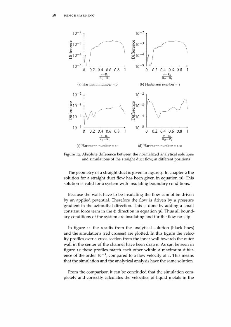
Figure 12: Absolute difference between the normalized analytical solutionsand simulations of the straight duct flow, at different positions
The geometry of a straight duct is given in figure 4. In chapter 2 thesolution for a straight duct flow has been given in equation 16. Thissolution is valid for a system with insulating boundary conditions.
Because the walls have to be insulating the flow cannot be drivenby an applied potential. Therefore the flow is driven by a pressuregradient in the azimuthal direction. This is done by adding a smallconstant force term in the φ direction in equation 36. Thus all bound-ary conditions of the system are insulating and for the flow no-slip.
In figure 11 the results from the analytical solution (black lines)and the simulations (red crosses) are plotted. In this figure the veloc-ity profiles over a cross section from the inner wall towards the outerwall in the center of the channel have been drawn. As can be seen infigure 12 these profiles match each other within a maximum differ-ence of the order 10−3, compared to a flow velocity of 1. This meansthat the simulation and the analytical analysis have the same solution.
From the comparison it can be concluded that the simulation com-pletely and correctly calculates the velocities of liquid metals in the
4.3 annular duct with square cross section 29
limit of small aspect ratios and laminar flows. This means that theboundary conditions have correctly been implemented.
4.3 annular duct with square cross section
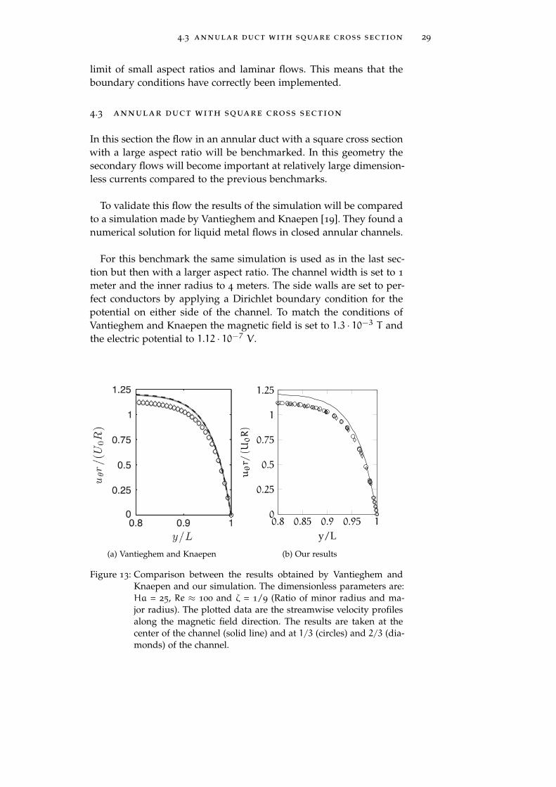
In this section the flow in an annular duct with a square cross sectionwith a large aspect ratio will be benchmarked. In this geometry thesecondary flows will become important at relatively large dimension-less currents compared to the previous benchmarks.
To validate this flow the results of the simulation will be comparedto a simulation made by Vantieghem and Knaepen [19]. They found anumerical solution for liquid metal flows in closed annular channels.
For this benchmark the same simulation is used as in the last sec-tion but then with a larger aspect ratio. The channel width is set to 1
meter and the inner radius to 4 meters. The side walls are set to per-fect conductors by applying a Dirichlet boundary condition for thepotential on either side of the channel. To match the conditions ofVantieghem and Knaepen the magnetic field is set to 1.3 · 10−3 T andthe electric potential to 1.12 · 10−7 V .
(a) Vantieghem and Knaepen
0.8 0.85 0.9 0.95 10
0.25
0.5
0.75
1
1.25
y/L
uθr/
( U0R)
(b) Our results
Figure 13: Comparison between the results obtained by Vantieghem andKnaepen and our simulation. The dimensionless parameters are:Ha = 25, Re ≈ 100 and ζ = 1/9 (Ratio of minor radius and ma-jor radius). The plotted data are the streamwise velocity profilesalong the magnetic field direction. The results are taken at thecenter of the channel (solid line) and at 1/3 (circles) and 2/3 (dia-monds) of the channel.
30 benchmarking
To be able to compare the solutions of the flow the same scalinghas to be applied on the velocity fields as Vantieghem and Knaepenhave done. The typical velocity is defined as:
U0 =V
B0R log R+LR−L
(44)
with:
R = radius at the center of the channel
L = half the channel width
In figure 13 the comparison is made. As can be seen in the graphsthe flow has the same velocity profile on the cross sections. The reduc-tion of the velocities at different positions in the channel also seemsto be the same, as can be seen by the position of the diamonds andcircles.
Besides the comparison of the primary flow the secondary flow canalso be compared. The secondary flow is defined as:
Us =√u2r + u
2z (45)
The secondary flow can be scaled, as is done in the paper of Vantieghemand Knaepen, but will not be done here because we are interested inthe qualitative behaviour of the secondary flow. In figure 14 the sec-ondary flow profiles are compared. Although it hard to exactly com-pare the two graphs because they have a slightly different perspectiveand plotting style. The shape of these figure appears to be largely thesame, with three peaks in both figures of the same size. These peaksare formed due to a vortex in the polodial plane. This vortex is thuspresent in both simulations, and appears to have the same character-istics.
Both simulations show the same behaviour in terms of velocity pro-files en secondary flows. This verifies that the simulation producesthe correct velocity profiles for both the primary and secondary flowin annular ducts.
From this chapter it can be concluded that the simulations pro-duces correct velocity profiles in axial symmetric geometries. Thebenchmarked simulations can now be used to determine the scalingbehaviour in annular ducts.

4.3 annular duct with square cross section 31
(a) Vantieghem and Knaepen
-1 0 1 0
1
0
2 · 10−6
(r− R) /Ly/L
Us
(b) Our results
Figure 14: Secondary flow comparison between the results obtained byVantieghem and Knaepen and our simulation. The dimensionlessparameters are: Ha = 25, Re ≈ 100 and ζ = 1/9 (Ratio of minorradius and major radius).

5M A G N E T O H Y D R O D Y N A M I C S C A L I N GB E H AV I O U R
In the introduction the goal has been stated to develop a simulationto study the scaling behaviour of the velocity flux at surface withthe electric and magnetic field in annular channels. To this end anumerical framework has been developed. This framework has beenvalidated, as described in chapter 4. Using this validated simulationthe scaling behaviour can be studied.
In chapter 2 three different types of scaling behaviours have beenidentified. The first area is the linear regime where the scaling of thevelocity flux is a linear function of the magnetic field and the appliedcurrent. The second regime is the magnetic braking regime where theflow is slowed by the magnetic field. The last regime is the secondaryflow regime where the secondary flows induced by the curvaturecause a sub-linear scaling of the velocity flux at the surface with themagnetic field and current.
To identify the different areas and to find the the values of the di-mensionless numbers at which the transition between the areas takesplace a simulation has been developed. Using this simulation the flowwill be studied. First this is done by studying the behaviour in singleannular channels, with vertical magnetic fields. The effects that whereobserved in the flow will be mentioned and explained. The form inwhich the results will be presented will also be explained in this sec-tion.
After that the complexity of the model is increased by using a mag-netic field with radial components. Further complexity is added byadding a fluid layer on top of the channels. The simulations are donein 2D, using an axial symmetric geometry and with the properties ofgalinstan, see page 26 for the values.
33

34 magnetohydrodynamic scaling behaviour
5.1 individual annular channels channels
5.1.1 Vertical magnetic field
5.1.1.1 Channel with an inner radius of 1 cm
In chapter 2 it has been described that the velocity flux at the surfaceis expected to scale linearly with the current and the magnetic field,at Hartmann numbers smaller than 1 (see 6, and relatively low flowrates. Besides the change in flow rate also the shape of the flow pro-file is expected to change. If the Hartmann number is increased thepeak velocity is expected to move towards the inner wall. Whereasthe peak is expected to move towards the outer wall for higher cur-rents.
10 15 20 250
2
4
r (mm)
z(m
m)
(a) Ha = 2.84 · 10−2, ID = 1.42
10 15 20 250
2
4
r (mm)
z(m
m)
(b) Ha = 2.84 · 101, ID = 8.81 · 10−5
10 15 20 250
2
4
r (mm)
z(m
m)
(c) Ha = 1.13, ID = 2.03 · 10−4
10 15 20 250
2
4
r (mm)
z(m
m)
(d) Ha = 2.84 · 10−2, ID = 5.64 · 10−5
10 15 20 250
2
4
r (mm)
z(m
m)
(e) Ha = 2.84 · 101, ID = 3.51 · 10−9
0 0.2 0.4 0.6 0.8 1
(f) Normalized velocity scale
Figure 15: Plot of normalized flow profiles for the inner channel at differentHa and ID. The combinations correspond to the extreme valuesof the Hartmann number and dimensionless current in the simu-lation and the median value.
5.1 individual annular channels channels 35
To visualise the change in behaviour for different dimensionlesscurrents and Hartmann numbers figure 15 is made from the resultsof the model. In these figures the normalized velocity profiles of thechannel with an inner radius of 1 cm are plotted for both the mini-mum and maximum current and magnetic field. Also the simulationwith the the median values of the simulated magnetic field and po-tential is plotted. The median value is taken instead of the averagebecause the simulations have a large range with logarithmic equidis-tant points. These solutions provide a qualitative understanding ofthe changes a flow gets from changing the magnetic field and poten-tial.
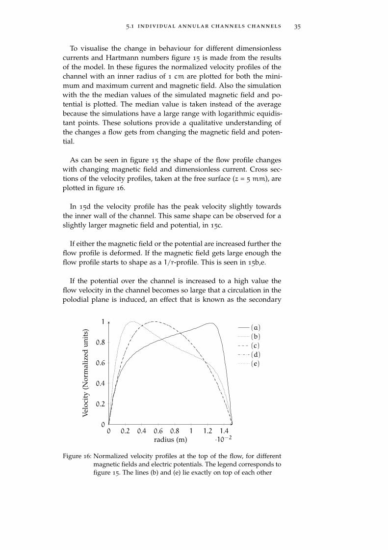
As can be seen in figure 15 the shape of the flow profile changeswith changing magnetic field and dimensionless current. Cross sec-tions of the velocity profiles, taken at the free surface (z = 5 mm), areplotted in figure 16.
In 15d the velocity profile has the peak velocity slightly towardsthe inner wall of the channel. This same shape can be observed for aslightly larger magnetic field and potential, in 15c.
If either the magnetic field or the potential are increased further theflow profile is deformed. If the magnetic field gets large enough theflow profile starts to shape as a 1/r-profile. This is seen in 15b,e.
If the potential over the channel is increased to a high value theflow velocity in the channel becomes so large that a circulation in thepolodial plane is induced, an effect that is known as the secondary
0 0.2 0.4 0.6 0.8 1 1.2 1.4·10−2
0
0.2
0.4
0.6
0.8
1
radius (m)
Velo
city
(Nor
mal
ized
unit
s)
(a)
(b)
(c)
(d)
(e)
Figure 16: Normalized velocity profiles at the top of the flow, for differentmagnetic fields and electric potentials. The legend corresponds tofigure 15. The lines (b) and (e) lie exactly on top of each other
36 magnetohydrodynamic scaling behaviour
10 12 14 16 18 20 22 240
2
4
r (mm)
z(m
m)
0 0.065 0.13 0.195 0.26
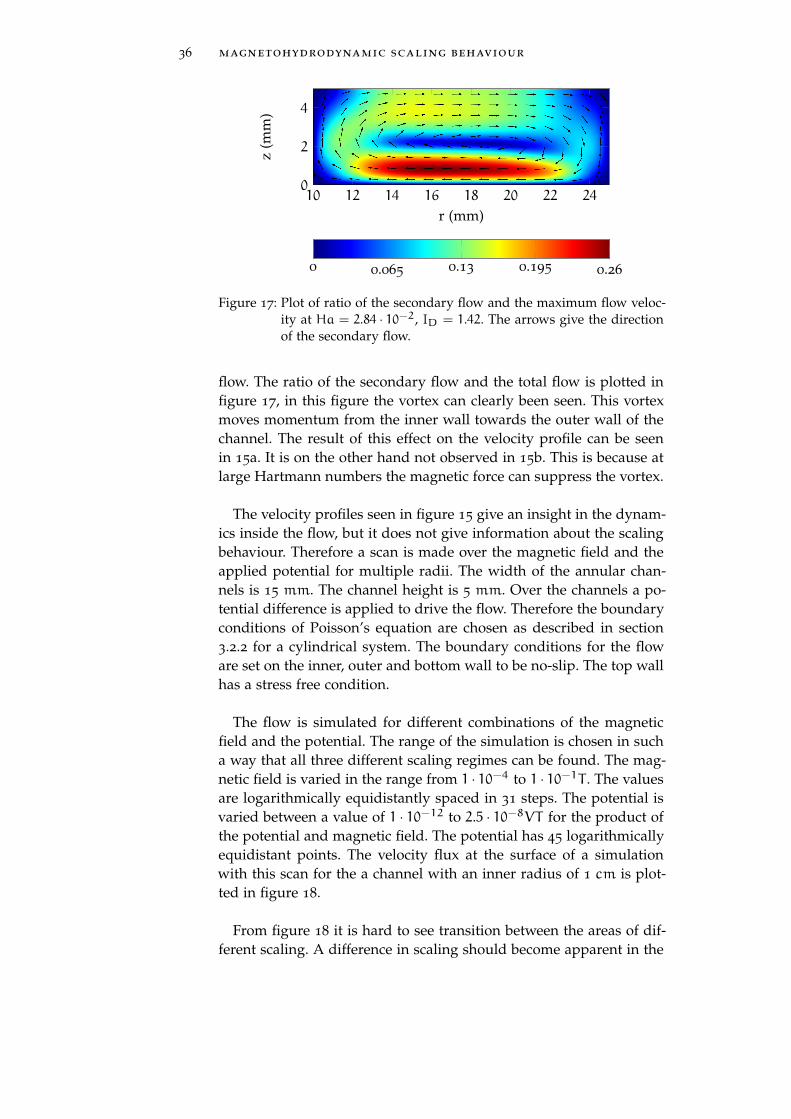
Figure 17: Plot of ratio of the secondary flow and the maximum flow veloc-ity at Ha = 2.84 · 10−2, ID = 1.42. The arrows give the directionof the secondary flow.
flow. The ratio of the secondary flow and the total flow is plotted infigure 17, in this figure the vortex can clearly been seen. This vortexmoves momentum from the inner wall towards the outer wall of thechannel. The result of this effect on the velocity profile can be seenin 15a. It is on the other hand not observed in 15b. This is because atlarge Hartmann numbers the magnetic force can suppress the vortex.
The velocity profiles seen in figure 15 give an insight in the dynam-ics inside the flow, but it does not give information about the scalingbehaviour. Therefore a scan is made over the magnetic field and theapplied potential for multiple radii. The width of the annular chan-nels is 15 mm. The channel height is 5 mm. Over the channels a po-tential difference is applied to drive the flow. Therefore the boundaryconditions of Poisson’s equation are chosen as described in section3.2.2 for a cylindrical system. The boundary conditions for the floware set on the inner, outer and bottom wall to be no-slip. The top wallhas a stress free condition.
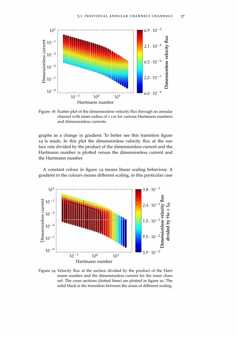
The flow is simulated for different combinations of the magneticfield and the potential. The range of the simulation is chosen in sucha way that all three different scaling regimes can be found. The mag-netic field is varied in the range from 1 · 10−4 to 1 · 10−1T . The valuesare logarithmically equidistantly spaced in 31 steps. The potential isvaried between a value of 1 · 10−12 to 2.5 · 10−8VT for the product ofthe potential and magnetic field. The potential has 45 logarithmicallyequidistant points. The velocity flux at the surface of a simulationwith this scan for the a channel with an inner radius of 1 cm is plot-ted in figure 18.
From figure 18 it is hard to see transition between the areas of dif-ferent scaling. A difference in scaling should become apparent in the
5.1 individual annular channels channels 37
10−1 100 10110−9
10−7
10−5
10−3
10−1
101
Hartmann number
Dim
ensi
onle
sscu
rren
t
Dim
ensi
onle
ssve
loci
tyflu
x
6.0 · 10−9
2.0 · 10−7
6.5 · 10−6
2.1 · 10−4
6.9 · 10−3
Dim
ensi
onle
ssve
loci
tyflu
x
Figure 18: Scatter plot of the dimensionless velocity flux through an annularchannel with inner radius of 1 cm for various Hartmann numbersand dimensionless currents.
graphs as a change in gradient. To better see this transition figure19 is made. In this plot the dimensionless velocity flux at the sur-face rate divided by the product of the dimensionless current and theHartmann number is plotted versus the dimensionless current andthe Hartmann number.
A constant colour in figure 19 means linear scaling behaviour. Agradient in the colours means different scaling, in this particular case
10−1 100 10110−9
10−7
10−5
10−3
10−1
101
Hartmann number
Dim
ensi
onle
sscu
rren
t
Dim
ensi
onle
ssve
loci
tyflu
xdi
vide
dbyHa×I D
5.9 · 10−2
9.5 · 10−2
1.5 · 10−1
2.4 · 10−1
3.8 · 10−1
Dim
ensi
onle
ssve
loci
tyflu
xdi
vide
dbyHa×I D
Figure 19: Velocity flux at the surface divided by the product of the Hart-mann number and the dimensionless current for the inner chan-nel. The cross sections (dotted lines) are plotted in figure 20. Thesolid black is the transition between the areas of different scaling.

38 magnetohydrodynamic scaling behaviour
10−1 100 10110−2
10−1
100
Hartmann number
Qs
ID×Ha
(a) Magnetic scan of figure 19
10−410−310−210−110−2
10−1
100
Dimensionless current
Qs
ID×Ha
(b) Electrical current scan of figure 19
10−1 100 101
10−6
10−4
10−2
Hartmann number
Qs
(c) Magnetic scan of figure 18
10−410−310−210−1
10−6
10−4
10−2
Dimensionless currentQs
(d) Electrical current scan of figure 18
Figure 20: Cross sections of figure 18 and 19. These cross sections representa scan over the Hartmann number and the dimensionless current.
sub-linear scaling. From this figure two cross sections are made. Inthe first cross section a scan is made over the magnetic field with aconstant current, in figure 19 the gray and white dotted line corre-sponds to this cross section. The plot of this cross section can be seenin figure 20a. A second sweep is made over the dimensionless currentwith a constant magnetic field, that is the vertical black and white dot-ted line. This is plotted in figure 20b. The same cross sections are alsomade in figure 18 and plotted as images 20c and d.
From the plots in figure 20 the scaling of the velocity flux can beobtained. First the scaling of the magnetic field can be seen, graph20a. A flat profile in this graph means linear scaling. As can be seenstarting from a Hartmann number of about 1 the function starts todecrease, and thus scales not linear anymore. In the plot 20b for thevelocity flux versus the current similar behaviour is observed. Start-ing from a dimensionless current of about 0.01 the velocity flux startsto decrease, and the scaling is not linear anymore. The non-linear scal-ing can also be observed in the plots of the velocity flux 20c and d,in these plots the gradients decrease when non-linear scaling is ob-served in plots 20a and b.
5.1 individual annular channels channels 39
A condition for the linearity of the scaling has been made to com-pare simulations with each other. The velocity flux divided by theproduct of the current and magnetic field does not scale linearly any-more when it is smaller than a certain threshold value. The algorithmanalysing the simulations uses the logarithm of the velocity flux, thethreshold value is set to 96% of the maximum value of the logarithmof the velocity flux at the surface, thus mathematically:
log(v)
max(log(v))
> 0.96, linear
< 0.96, non-linear(46)
Or in the non logarithmic case:
v
max(v)
> 0.912, linear
< 0.912, non-linear(47)
This value was chosen because from this point it was obvious thatthe scaling was not linear anymore. The output data has a fairly poorresolution, therefore a first order interpolation is used to determinethe threshold values more exactly. This can be done since the flux isalways monotonically decreasing in the transition area with respectto increasing Hartmann number or dimensionless current.
The result for this threshold is plotted in figure 19 as a black line.This line is the boundary between linear and non-linear scaling. Thearea to the left and below the line is the area that scales linearly. Tothe right of this curve the magnetic force slows the fluid down. Non-linear scaling above the line is due to the secondary flow induced bythe curvature of the channel.
The scaling of the function can be obtained from the rate of changein figure 18. To determine the scaling the following function is as-sumed between to successive points in the plot:
y = b · xa (48)
In this case y is the dimensionless velocity flux, b is a scaling constant,x is either the Hartmann number or the dimensionless current, and fi-nally a is the power to which the function scales. From this function itis possible to determine the power a. This is done using the followingcalculation: First the ratio between two points is taken:
y2y1
=b · xa2b · xa1
(49)
And from this the power a can easily be obtained:
a =ln (y2/y1)
ln (x2/x1)(50)
40 magnetohydrodynamic scaling behaviour
10−1 100 101
10−8
10−6
10−4
10−2
100
Hartmann number
Dim
ensi
onle
sscu
rren
t0.2
0.4
0.6
0.8
1
Pow
era
(a) Scaling in the direction of the Hartmann number
10−1 100 101
10−8
10−6
10−4
10−2
100
Hartmann number
Dim
ensi
onle
sscu
rren
t
0.7
0.8
0.9
1
Pow
era
(b) Scaling in the direction of the dimensionless current
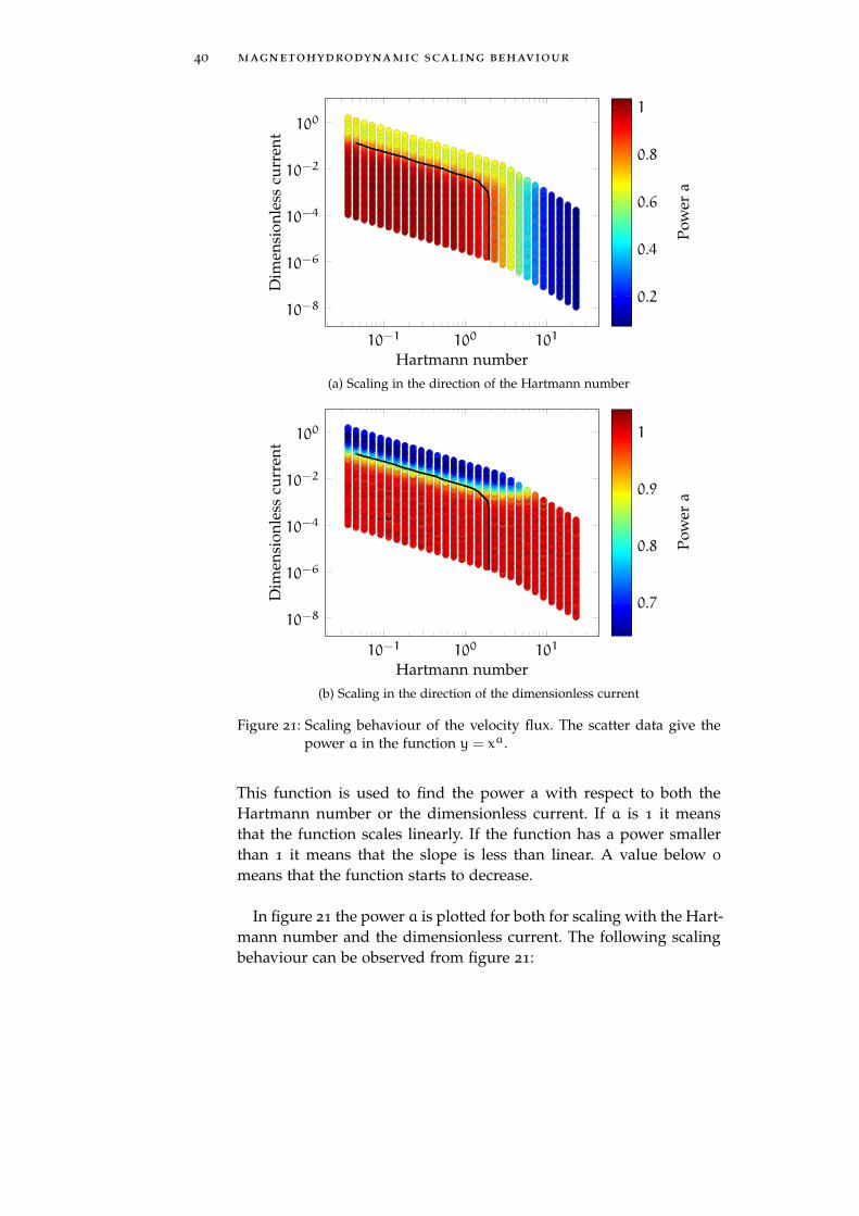
Figure 21: Scaling behaviour of the velocity flux. The scatter data give thepower a in the function y = xa.
This function is used to find the power a with respect to both theHartmann number or the dimensionless current. If a is 1 it meansthat the function scales linearly. If the function has a power smallerthan 1 it means that the slope is less than linear. A value below 0
means that the function starts to decrease.
In figure 21 the power a is plotted for both for scaling with the Hart-mann number and the dimensionless current. The following scalingbehaviour can be observed from figure 21:
5.1 individual annular channels channels 41
• Linear scaling for small Hartmann number and dimensionlesscurrent
• Sub-linear scaling for large dimensionless currents and smallHartmann numbers
• Sub-linear scaling for large Hartmann numbers
This scaling is in agreement with what was expected in chapter 2.
5.1.1.2 Channel with larger inner radii
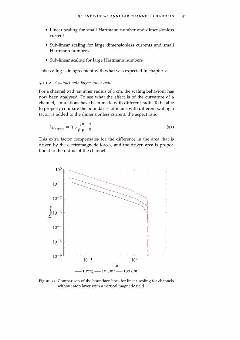
For a channel with an inner radius of 1 cm, the scaling behaviour hasnow been analysed. To see what the effect is of the curvature of achannel, simulations have been made with different radii. To be ableto properly compare the boundaries of mains with different scaling afactor is added to the dimensionless current, the aspect ratio:
IDaspect = Iµ0
√σ
µ· aR
(51)
This extra factor compensates for the difference in the area that isdriven by the electromagnetic forces, and the driven area is propor-tional to the radius of the channel.
10−1 10010−6
10−5
10−4
10−3
10−2
10−1
100
Ha
I Daspect
1 cm; 10 cm; 100 cm
Figure 22: Comparison of the boundary lines for linear scaling for channelswithout atop layer with a vertical magnetic field.
42 magnetohydrodynamic scaling behaviour
In figure 22 the boundary between linear and non-linear scalingis plotted for an inner channel radius of 1, 10 and 100 cm. The scal-ing has for all channels a very similar shape. For the magnetic scal-ing behaviour a vertical boundary is found, at nearly the same place,around Ha = 2. The boundary for non-linear scaling due to the curva-ture is found on lines of constant J× B. The lines differ for differentchannel diameters. For larger diameters of the channels the linearscaling is observed for higher dimensionless currents. This is alsowhat was expected, as the circulation is induced by the curvature ofthe channel. This effect happens more easily in channels with smallerdiameters, reducing the velocity. This results in non-linear scaling atlower currents.
5.1.2 Realistic magnetic field
In the previous section a method has been introduced to character-ize the areas of different scaling in individual annular channels witha vertical magnetic field. In this section the effects of a realistic mag-netic field are studied. To do this the magnetic fields module is addedto the simulation to facilitate the calculation of a more realistic mag-netic field.
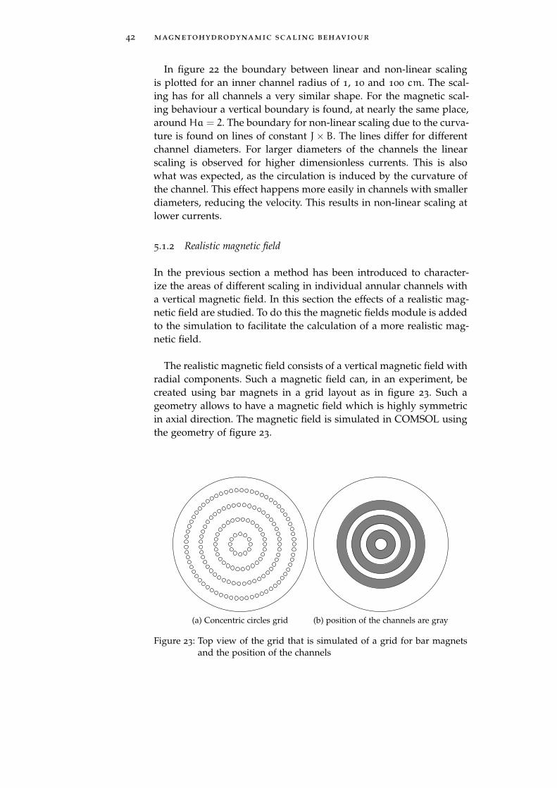
The realistic magnetic field consists of a vertical magnetic field withradial components. Such a magnetic field can, in an experiment, becreated using bar magnets in a grid layout as in figure 23. Such ageometry allows to have a magnetic field which is highly symmetricin axial direction. The magnetic field is simulated in COMSOL usingthe geometry of figure 23.
(a) Concentric circles grid (b) position of the channels are gray
Figure 23: Top view of the grid that is simulated of a grid for bar magnetsand the position of the channels
5.1 individual annular channels channels 43
SlipNo-slipSymmetry
10 mm 15 mm 15 mm 15 mm
height MagnetsAir
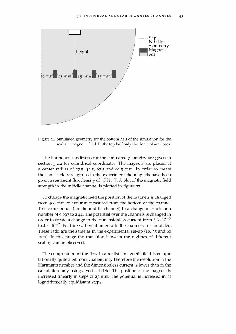
Figure 24: Simulated geometry for the bottom half of the simulation for therealistic magnetic field. In the top half only the dome of air closes.
The boundary conditions for the simulated geometry are given insection 3.2.2 for cylindrical coordinates. The magnets are placed ata center radius of 27.5, 42.5, 67.5 and 92.5 mm. In order to createthe same field strength as in the experiment the magnets have beengiven a remanent flux density of 1.73ez T . A plot of the magnetic fieldstrength in the middle channel is plotted in figure 27.
To change the magnetic field the position of the magnets is changedfrom 400 mm to 150 mm measured from the bottom of the channel.This corresponds (for the middle channel) to a change in Hartmannnumber of 0.097 to 2.44. The potential over the channels is changed inorder to create a change in the dimensionless current from 5.6 · 10−5to 3.7 · 10−2. For three different inner radii the channels are simulated.These radii are the same as in the experimental set-up (10, 35 and 60
mm). In this range the transition between the regimes of differentscaling can be observed.
The computation of the flow in a realistic magnetic field is compu-tationally quite a bit more challenging. Therefore the resolution in theHartmann number and the dimensionless current is lower than in thecalculation only using a vertical field. The position of the magnets isincreased linearly in steps of 25 mm. The potential is increased in 11
logarithmically equidistant steps.
44 magnetohydrodynamic scaling behaviour
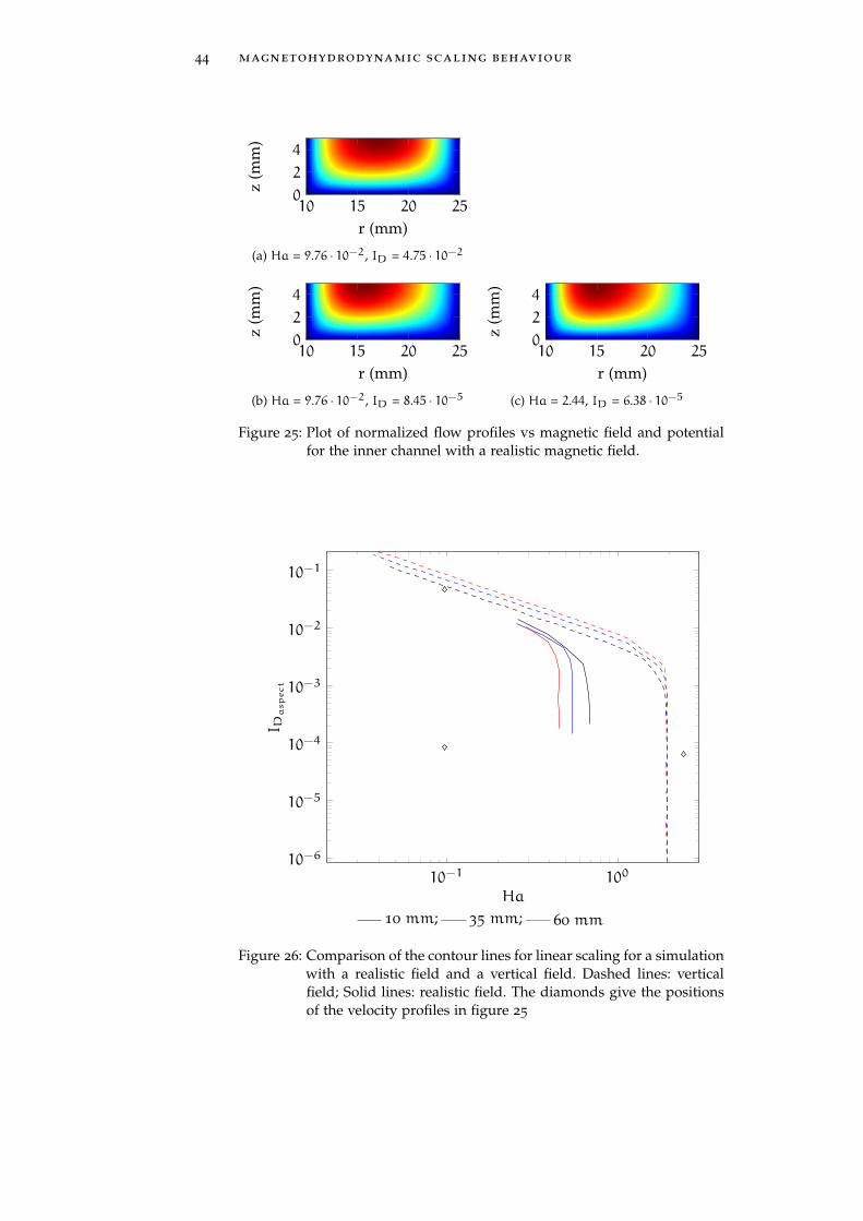
10 15 20 250
2
4
r (mm)
z(m
m)
(a) Ha = 9.76 · 10−2, ID = 4.75 · 10−2
10 15 20 250
2
4
r (mm)
z(m
m)
(b) Ha = 9.76 · 10−2, ID = 8.45 · 10−5
10 15 20 250
2
4
r (mm)
z(m
m)
(c) Ha = 2.44, ID = 6.38 · 10−5
Figure 25: Plot of normalized flow profiles vs magnetic field and potentialfor the inner channel with a realistic magnetic field.
10−1 10010−6
10−5
10−4
10−3
10−2
10−1
Ha
I Daspect
10 mm; 35 mm; 60 mm
Figure 26: Comparison of the contour lines for linear scaling for a simulationwith a realistic field and a vertical field. Dashed lines: verticalfield; Solid lines: realistic field. The diamonds give the positionsof the velocity profiles in figure 25
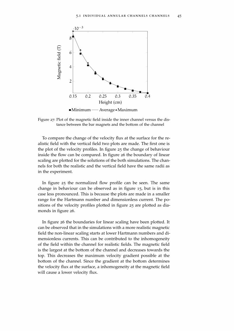
5.1 individual annular channels channels 45
0.15 0.2 0.25 0.3 0.35 0.4
2
4
6
8
·10−3
Height (cm)
Mag
neti
cfie
ld(T
)
Minimum Average Maximum
Figure 27: Plot of the magnetic field inside the inner channel versus the dis-tance between the bar magnets and the bottom of the channel
To compare the change of the velocity flux at the surface for the re-alistic field with the vertical field two plots are made. The first one isthe plot of the velocity profiles. In figure 25 the change of behaviourinside the flow can be compared. In figure 26 the boundary of linearscaling are plotted for the solutions of the both simulations. The chan-nels for both the realistic and the vertical field have the same radii asin the experiment.
In figure 25 the normalized flow profile can be seen. The samechange in behaviour can be observed as in figure 15, but is in thiscase less pronounced. This is because the plots are made in a smallerrange for the Hartmann number and dimensionless current. The po-sitions of the velocity profiles plotted in figure 25 are plotted as dia-monds in figure 26.
In figure 26 the boundaries for linear scaling have been plotted. Itcan be observed that in the simulations with a more realistic magneticfield the non-linear scaling starts at lower Hartmann numbers and di-mensionless currents. This can be contributed to the inhomogeneityof the field within the channel for realistic fields. The magnetic fieldis the largest at the bottom of the channel and decreases towards thetop. This decreases the maximum velocity gradient possible at thebottom of the channel. Since the gradient at the bottom determinesthe velocity flux at the surface, a inhomogeneity at the magnetic fieldwill cause a lower velocity flux.
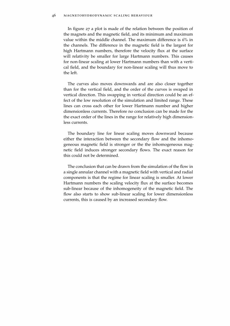
46 magnetohydrodynamic scaling behaviour
In figure 27 a plot is made of the relation between the position ofthe magnets and the magnetic field, and its minimum and maximumvalue within the middle channel. The maximum difference is 6% inthe channels. The difference in the magnetic field is the largest forhigh Hartmann numbers, therefore the velocity flux at the surfacewill relativity be smaller for large Hartmann numbers. This causesfor non-linear scaling at lower Hartmann numbers than with a verti-cal field, and the boundary for non-linear scaling will thus move tothe left.
The curves also moves downwards and are also closer togetherthan for the vertical field, and the order of the curves is swaped invertical direction. This swapping in vertical direction could be an ef-fect of the low resolution of the simulation and limited range. Theselines can cross each other for lower Hartmann number and higherdimensionless currents. Therefore no conclusion can be made for thethe exact order of the lines in the range for relatively high dimension-less currents.
The boundary line for linear scaling moves downward becauseeither the interaction between the secondary flow and the inhomo-geneous magnetic field is stronger or the the inhomogeneous mag-netic field induces stronger secondary flows. The exact reason forthis could not be determined.
The conclusion that can be drawn from the simulation of the flow ina single annular channel with a magnetic field with vertical and radialcomponents is that the regime for linear scaling is smaller. At lowerHartmann numbers the scaling velocity flux at the surface becomessub-linear because of the inhomogeneity of the magnetic field. Theflow also starts to show sub-linear scaling for lower dimensionlesscurrents, this is caused by an increased secondary flow.
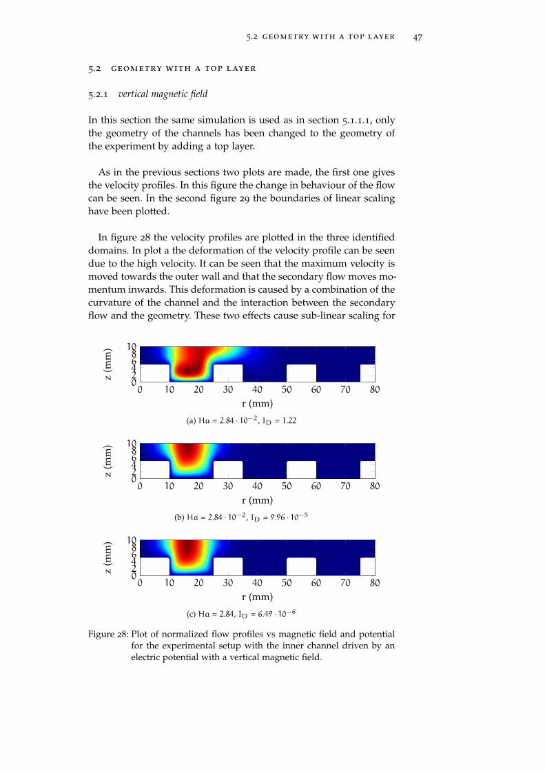
5.2 geometry with a top layer 47
5.2 geometry with a top layer
5.2.1 vertical magnetic field
In this section the same simulation is used as in section 5.1.1.1, onlythe geometry of the channels has been changed to the geometry ofthe experiment by adding a top layer.
As in the previous sections two plots are made, the first one givesthe velocity profiles. In this figure the change in behaviour of the flowcan be seen. In the second figure 29 the boundaries of linear scalinghave been plotted.
In figure 28 the velocity profiles are plotted in the three identifieddomains. In plot a the deformation of the velocity profile can be seendue to the high velocity. It can be seen that the maximum velocity ismoved towards the outer wall and that the secondary flow moves mo-mentum inwards. This deformation is caused by a combination of thecurvature of the channel and the interaction between the secondaryflow and the geometry. These two effects cause sub-linear scaling for
0 10 20 30 40 50 60 70 800246810
r (mm)
z(m
m)
(a) Ha = 2.84 · 10−2, ID = 1.22
0 10 20 30 40 50 60 70 800246810
r (mm)
z(m
m)
(b) Ha = 2.84 · 10−2, ID = 9.96 · 10−5
0 10 20 30 40 50 60 70 800246810
r (mm)
z(m
m)
(c) Ha = 2.84, ID = 6.49 · 10−6
Figure 28: Plot of normalized flow profiles vs magnetic field and potentialfor the experimental setup with the inner channel driven by anelectric potential with a vertical magnetic field.

48 magnetohydrodynamic scaling behaviour
10−1 10010−6
10−5
10−4
10−3
10−2
10−1
100
Ha
I Daspect
10 mm; 35 mm; 60 mm
Figure 29: Comparison of the boundary lines for linear scaling for a simu-lation with a realistic field and a vertical field. Dashed lines: in-dividual channels; solid lines: experimental set-up with a verticalmagnetic field.
a lower product of the Hartmann number and the dimensionless cur-rents. In figure b were neither magnetic braking or curvature effects.In this regime the flow scales linearly. In figure c magnetic brakingdominates the flow, in the bulk layer on top the magnetic field alsoslows down the flow. This results in a small change in the velocityprofile, the profile is slightly more leveled in plot c than in b. Thiscauses non-linear scaling for the velocity flux at the surface, an effectthat can also be observed in figure 29. In this figure the boundaryfor linear scaling moves to the left, i.e. non-linear scaling happens al-ready for smaller Hartmann numbers.
From these results it can be concluded that the geometry reducesthe regime of linear scaling both from the magnetic braking as thesecondary flow side. The shape of this area stays the same.
The method used to simulate these flows does not yield errors inthe simulated domain. However when the current is increased prob-lems can occur. This problem arises because it is difficult for COM-SOL to compute accurate boundary fluxes in diffusion dominatedproblems. The increase the domain which simulation can be madethe corners have been rounded with a radius of 0.5 mm in the simu-lation. This allowed for consistent calculations, but still in a relativity
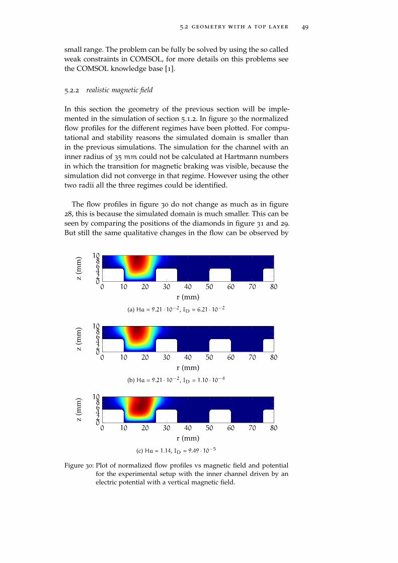
5.2 geometry with a top layer 49
small range. The problem can be fully be solved by using the so calledweak constraints in COMSOL, for more details on this problems seethe COMSOL knowledge base [1].
5.2.2 realistic magnetic field
In this section the geometry of the previous section will be imple-mented in the simulation of section 5.1.2. In figure 30 the normalizedflow profiles for the different regimes have been plotted. For compu-tational and stability reasons the simulated domain is smaller thanin the previous simulations. The simulation for the channel with aninner radius of 35 mm could not be calculated at Hartmann numbersin which the transition for magnetic braking was visible, because thesimulation did not converge in that regime. However using the othertwo radii all the three regimes could be identified.
The flow profiles in figure 30 do not change as much as in figure28, this is because the simulated domain is much smaller. This can beseen by comparing the positions of the diamonds in figure 31 and 29.But still the same qualitative changes in the flow can be observed by
0 10 20 30 40 50 60 70 800246810
r (mm)
z(m
m)
(a) Ha = 9.21 · 10−2, ID = 6.21 · 10−2
0 10 20 30 40 50 60 70 800246810
r (mm)
z(m
m)
(b) Ha = 9.21 · 10−2, ID = 1.10 · 10−4
0 10 20 30 40 50 60 70 800246810
r (mm)
z(m
m)
(c) Ha = 1.14, ID = 9.49 · 10−5
Figure 30: Plot of normalized flow profiles vs magnetic field and potentialfor the experimental setup with the inner channel driven by anelectric potential with a vertical magnetic field.
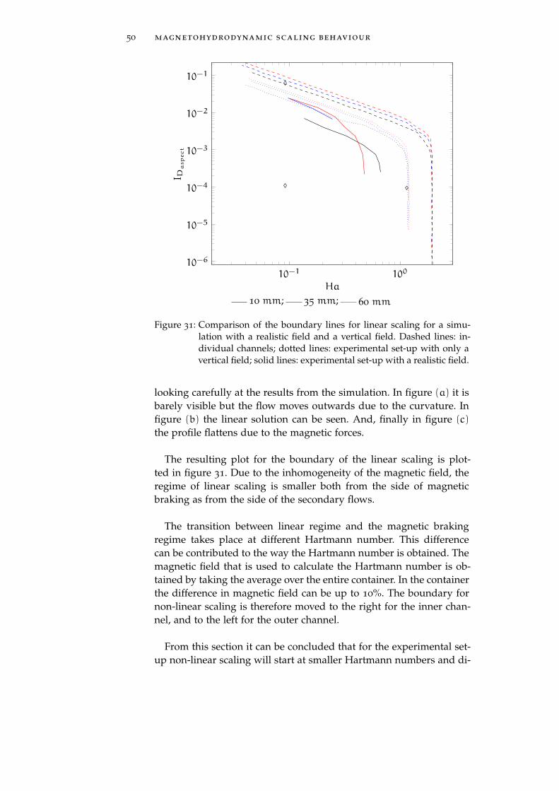
50 magnetohydrodynamic scaling behaviour
10−1 10010−6
10−5
10−4
10−3
10−2
10−1
Ha
I Daspect
10 mm; 35 mm; 60 mm
Figure 31: Comparison of the boundary lines for linear scaling for a simu-lation with a realistic field and a vertical field. Dashed lines: in-dividual channels; dotted lines: experimental set-up with only avertical field; solid lines: experimental set-up with a realistic field.
looking carefully at the results from the simulation. In figure (a) it isbarely visible but the flow moves outwards due to the curvature. Infigure (b) the linear solution can be seen. And, finally in figure (c)
the profile flattens due to the magnetic forces.
The resulting plot for the boundary of the linear scaling is plot-ted in figure 31. Due to the inhomogeneity of the magnetic field, theregime of linear scaling is smaller both from the side of magneticbraking as from the side of the secondary flows.
The transition between linear regime and the magnetic brakingregime takes place at different Hartmann number. This differencecan be contributed to the way the Hartmann number is obtained. Themagnetic field that is used to calculate the Hartmann number is ob-tained by taking the average over the entire container. In the containerthe difference in magnetic field can be up to 10%. The boundary fornon-linear scaling is therefore moved to the right for the inner chan-nel, and to the left for the outer channel.
From this section it can be concluded that for the experimental set-up non-linear scaling will start at smaller Hartmann numbers and di-

5.2 geometry with a top layer 51
mensionless currents, than what would be expected from strait ductsor closed annular channels.

6C O N C L U S I O N , D I S C U S S I O N A N D O U T L O O K
6.1 conclusion
In this thesis the influence of a top layer on scaling behaviour of thevelocity flux at the surface of a liquid metal flow with the Hartmannnumber and dimensionless current was studied in annular channels.The following conclusion can be drawn from the work:
A simulation, using the magnetohydrodynamic theory, has beendeveloped that can simulate a flow of a liquid metal in an arbitrarygeometry. This model has been validated in axial symmetric channelsusing benchmarks from literature. With this simulation it is possibleto study the influence of top layer on the scaling behaviour of thevelocity flux at the surface with the magnetic field and the electriccurrent.
This simulation, in combination with a theoretical analysis, has firstbeen used to identify three areas of different scaling in a single an-nular channel. It was found that for small Hartmann numbers anddimensionless currents the velocity flux at the surface scales linearlywith the electric current and magnetic field. If either the Hartmannnumber or the dimensionless current is increased it was found thatthe flow velocity flux at the surface does not scale linearly anymore.
The velocity flux at the surface does not scale linearly with increas-ing Hartmann number because at large Hartmann numbers. This be-cause currents that are induced by the flow, of a metal, through amagnetic field cause a braking force in the flow. This effect starts inindividual channels without a top layer to dominate the flow for aHartmann number of about two. The start of this effect is indepen-dent of the inner radius of a channel.
If the product of the magnetic field and the current becomes toolarge at small Hartmann numbers secondary flows begin to influencethe velocity flux at the surface. These secondary flows are inducedby the curvature of the channels. The scaling of the velocity flux isreduced to sub-linear above certain values of the product of the Hart-mann number and the dimensionless currents. This value depends onthe radius of the channel: From a value of 5.5 · 10−3 AT for an innerradius of 1 cm to 3.2 · 10−2 AT for a channel with a inner radius of100 cm, whereby the dimensionless current is adjusted for the differ-
53
54 conclusion, discussion and outlook
ence in aspect ratio.
If a top layer is added to the channels, both the current and the floware changed. However in this geometry the same three areas are ob-served. The place where the transition between these areas takes placeis changed. Magnetic braking becomes dominant for lower Hartmannnumbers, it happens for about half the Hartmann number comparedto an individual channel. The non-linear scaling of the velocity fluxat the surface at lower Hartmann number occurs because also in thetop layer currents are induced, and just as in the channels they causebraking of the flow.
The influence of the secondary flows becomes also more dominantat lower values of the product of the Hartmann number and dimen-sionless current. The change is larger for the outer channel than forthe inner channel. The product of the dimensionless current and theHartmann number for which the change takes place is about threetimes lower for the outer channel and two times lower for the innerchannel, again adjusted for the difference in aspect ratio.
Besides the main question the additional question was: How doesthe scaling of the velocity flux at the surface change if the magneticfield is is not perfectly parallel and perpendicular to the surface. Toanswer this a simulation was made in which the magnetic field wasmade using bar magnets. From the results of the simulation it wasfound that a non-homogeneous magnetic field does significantly in-fluence the scaling with the Hartmann number and dimensionlesscurrent, both in individual channels and in the system with the toplayer.
For both the individual channel and the system with the top layerthe same changes to the scaling were found. Magnetic braking oc-curred for much lower Hartmann numbers, the change was in indi-vidual channels from 2 to around 0.5. The start of the transition be-tween the linear scaling and the magnetic braking does now dependon the radius. This is because of the difference in homogeneity of themagnetic field in the channels.
For the system with the experimental set-up a very similar changeis seen from about 1 to 0.4. The reason that the magnetic braking hap-pens at a lower Hartmann number is due to the fact that the magneticfield is not homogeneous anymore, it is strongest at the bottom of thechannel. Therefore the maximum gradient of the velocity profile islimited more in the bottom of the channel than it would be with aparallel magnetic field, and thus the resulting velocity is lower.
6.2 discussion 55
The secondary flow also becomes more important at lower valueof the product of the magnetic field and the dimensionless current.Therefore there appears to be a coupling between the non-homogeneousmagnetic field and the secondary flow.
6.2 discussion
The simulations were made in the idealized case, in reality other ef-fects come into play, due slightly different geometry and boundaryconditions, also the range can be extended to fully incorporate thepotential experimental regime.
The simulated geometry of the experimental set-up is slightly changedfrom the real set-up. The corners were rounded to ensure a correctflux calculation of the potential. This could have an influence on thecalculated flow as the secondary flow has to follow a surface withoutsharp corners in the simulation opposed to the experiment. Anothersolution to this problem to used the so-called weak constraints inCOMSOL for the calculation of the boundary fluxes. The weak con-straints would also allow to extend the range in which simulationscan be made to higher Hartmann numbers and dimensionless cur-rents.
The boundary conditions that are used to simulate the current re-stricted the simulation to perfectly conducting boundary conditionsfor the walls where the potential is applied and insulating for theother walls. These conditions are not necessarily met in experimen-tal set-ups, especially not the perfectly conducting walls. In a channelwith walls with a finite conductivity the volumetric rate is higher thanthrough a channel with a perfectly conductive wall.
Due to the choice of the modules in COMSOL the simulations hada limited regime in which they could be preformed. The model islimited in the range of the driving terms (current and magnetic field),if they become too large the flow can become unstable this can eitherbe due to the development of turbulence or due to numerical insta-bilities. The simulation has been developed to cope with turbulence.To extend the simulation to the flow in this regime the turbulent flowmodule can be used in COMSOL.
It was found from the simulations that there was a coupling be-tween the secondary flow and the inhomogeneous magnetic field. Butno reason has been found to what caused this. A possible explanationcould be that the gradient of the magnetic field increase the pressuregradient that is needed to keep the flow following the curved channel.This pressure gradient causes the secondary flow, a coupling between
56 conclusion, discussion and outlook
the two gradients could act as an initiator of a stronger secondaryflow.
6.2.1 Comparison with other MHD simulation codes
The simulation described in this report has been developed to sim-ulated liquid metal flows in COMSOL. The model is validated bya comparison with two analytic solutions and a model published byVantieghem and Knaepen. These benchmarks showed that the simula-tion is capable of correctly calculating velocity fields of laminar liquidmetal flows. The simulation can do this in an arbitrary geometries (aslong as enough computer power is available). In the simulation extraphysics can easily be implemented by adding other modules in COM-SOL.
Besides the simulation that we developed other codes have beendeveloped to simulated MHD-flows. The two most well known codesare: HIMAG and YALES2.
HIMAG is a code developed at UCLA, and it is currently beingdistributed by a company called Hypercomp [9]. UCLA’s goal wasto design a liquid lithium wall for a fusion reactor. HIMAG is usedto simulate this liquid wall. The code is designed to simulate com-plex free surface liquid metal MHD flows. The algorithm allows: anygeometry; high Hartmann numbers; thin Hartmann layers and par-allel solving. Their work differed from the simulation presented inthis report, as they focussed on higher Hartmann numbers and de-formable free surfaces (e.g. waves). This allows for simulations thatare better suited for calculations in a tokamak. The main reason forthis is that the magnetic fields are strong in tokamaks and thereforethe Hartmann numbers are typically high. However no calculationshave been published using HIMAG in a comparable geometry to oursand with similar Hartmann numbers.
YALES2 is another code that is available and capable of solvingthe MHD-equations [19]. YALES2 has originally been developed byCoria to simulated two phase combustion (e.g. for simulations ofengines). YALES2 also has a library that is capable of solving theMHD-equation. This has been used by Vantieghem and Knaepen tocalculated a liquid metal flow in various geometries. One of thesegeometries was a closed annular duct with square cross section. Inchapter 4 these results were used to validated our simulation. Theirwork mainly focused on flows with high Hartmann numbers andReynolds numbers, to study magnetic suppression of turbulence.

6.3 future directions 57
Besides these stand alone MHD-codes there have also been a num-ber of attempts to simulated a liquid metal flow in COMSOL. Thishas been done in the group of Gutierrez-Miravete at department ofEngineering and Science at the Rensealear polytechnic institute inHartford. The goal of these simulations was to simulated heat trans-fer in liquid metal flow for industrial applications in COMSOL. To dothis both simulations of a flow between parallel plates [4] and over abackward step [20] were made in COMSOL. They showed that COM-SOL simulations can accurately reproduce theoretical expectations ofliquid metal flows, but are less advanced than the simulations ex-plained in this report. Their simulations were only used to simulateliquid metal flows in simple geometries with vertical magnetic fields.Whereas our simulations can use much more complex geometries andboundary conditions.
The main difference between HIMAG, YALES2 and our simulationis that COMSOL allows to add other physics. With this flexibility sim-ulations of combined physical phenomena can be made. This allowsfor the use of our code in simulations that are relevant for liquidmetal flows in nuclear fusion applications. Examples of physics thatcan be added is the influence of the plasma on the liquid metal or theresponse of a liquid metal to transient heat loads of ELMs.
6.3 future directions
6.3.1 Simulations
The simulations have been used to find the boundary lines for the dif-ferent scaling regimes. But the simulations are able to do much morethan that. As a first step the simulations can be used to predict the re-sults of the experimental set-up. Making a simulation with the sameboundary conditions as the experiment can be used to validate thesimulation in a range in which it has not yet been validated. To fullyeclipse the experimental range the simulation has to be expandedwith the incorporation of the weak constraints to enforce a correct cal-culation of the boundary fluxes at large Hartmann numbers. If thisdoes not expand the operational domain of the simulation enough,because the flow is turbulent, the turbulent flow module of COMSOLmight need to be used.
Also simulations can be made in different geometries. A possiblegood starting point would be to simulate geometries in which alreadyrelevant experiments and simulations have been done. An exampleof this would be the MTOR experiment of Princeton [10], this ex-periment has also been simulated using HIMAG. In this experimenta flow of galinstan on an inclined plane in strong magnetic fields
58 conclusion, discussion and outlook
has been studied. This experiment has been done to study the be-haviour of liquid metal flow for divertor purposes. A positive matchbetween this experiment and the simulations would extend the do-main in which the simulation is benchmarked into the domain whereit is relevant for fusion applications.
6.3.2 Liquid metal divertor
Two possible mechanism can be used to transport the heat out of aliquid metal divertor: conduction and convection. The liquid metallayer acts, in the case of conduction, as a protection layer for the di-vertor. The heat is transported through the liquid metal layer andthe heat exchanger below it by means of conduction. The amount ofheat that is conducted through such a layer can be calculated usingFourier’s law
(qx = λ∂T∂x
). From this relation it can be seen that the
amount of heat conduction is proportional to the temperature differ-ence. The temperature at the surface is in this case the limiting factor.This is because liquid metals have a maximum temperature beforethey start too evaporate to fast. The flow of a liquid metal is onlyneeded to refresh the material. The material must be refreshed be-cause the material slowly evaporates. The flow velocities are smallerthan for which our simulation is designed.
The second mechanism to transport heat is through convection. Inthis case the flow transports the heat out of the divertor. In this casethe heat load is still limited by the maximum temperature of the liq-uid metal, but not solely through Fourier’s law. The temperature in-crease is also determined by the heat capacity of the metal and thetime the metal is exposed to the heat flux. This time can be limited bya fast flow. In this type of liquid metal divertor it could be useful tohave an active control.
As mentioned in the introduction local control of the flow in thedivertor could be used to increase the self healing capability of thedivertor, but that is nothing new. What our results show is that it isnow know when the liquid metal in the divertor is in certain scalingregimes. To be able to change between the linear scaling regime andthe other regimes the Hartmann number should be below one. Typi-cal values in a tokamak are a magnetic field of about 5 T , in the calcu-lation of the Hartmann number the perpendicular component to theflow is important. Since the surface of the divertor typically makesa very small angle with the magnetic field lines this field is easilyreduced by a factor of 10, leaving an effective field left of 0.5 T . Toget a Hartmann number of one the channel width for galinstan is 50
µm. This is too small to be useful, thus therefore the flow is always inthe regime of magnetic braking. The channel width for lithium would
6.3 future directions 59
even be lower as is a better conductor and less viscous than galinstan.
It could be beneficial to have a secondary flow in the divertor, e.g.it could for example lower the recycling. The recycling is improvedbecause the material will saturate slower. To enforce a secondary flowat large Hartmann numbers a larger current is needed than to drivethe flow without a secondary flow. In the simulated regime it was ob-served that the magnetic field suppressed the secondary flow. There-fore no criteria has been found for the transition between the mag-netic braking area and the secondary flow area. But it can be con-cluded from the simulations that the boundary is for larger productsof the dimensionless currents and Hartmann numbers than used inthe simulation.
Realistically the liquid metal divertor will be in the regime of mag-netic braking, a secondary flow might be induced by using large cur-rents.
Our work has also generated some generic results which mighthave applications beyond the scope of nuclear fusion. An exampleis the use of the stress free surface of the liquid metal for mirrorapplications. These mirrors made with liquid metals allow for veryflat and reflective mirrors. A example of such a mirror is a liquidmetal telescope, a round bath is rotated to create a parabolic mirror.The simulations can be used to calculate if it is possible to make aparabolic mirror with a set-up like the one that was used in the exper-iment. Benefits of such a system would be that there are no movingparts resulting in less vibrations.

AB U C K I N G H A M ’ S Π T H E O R E M
The Buckingham’s Π theorem is a procedure to create a complete setof independent dimensionless variables of a problem. This set can beused to see how a problem scales. In this sense it is used for the flowin annular channels. In the simulations the scaling behaviour of thevelocity flux will be studied. The dimensionless parameters of thisproblem will be derived in this chapter.
The velocity flux is a function of:
Q s = f ( v , ρ , µ , a , I , B , σ , µm ) (52)
These variables have the following dimensions:
[Q s ] = L 3 T −1 ; [ v ] = L T −1 ; [ρ ] = ML−3 ; (53)
[µ ] = ML−1 T −1 ; [a ] = L ; [ I ] = I ;
[B ] = I−1MT −2 ; [σ ] = M−1 L−3 T 3 I 2 ;
[µm ] = MLT −2 I−2
There are nine variables and four physical quantities (length, time,mass and current). According to Buckingham’s Π theorem there are(9 - 4) = 5 independent dimensionless numbers. These numbers canbe obtained from this function:
Π = Qa1s va2 ρa3µa4 aa5 Ia6Ba7 σa8µa9m (54)
To make Π dimensionless the parameters a have to be chosen cor-rectly. This restriction leads to the following equation for the basedimensions:
M: a3 + a4 + a7 − a8 + a9 = 0 (55)
L: 3a 1 + a2 − 3a 3 − a4 + a5 − 3a 8 + a9 = 0 (56)
T: − a1 − a2 − a4 − 2a 7 + 3a 8 − 2a 9 = 0 (57)
I: a6 − a7 + 2a 8 − 2a 9 = 0 (58)
As repeating variable (µ , a , σ , µm ) are chosen. Since that of thevelocity flux the relations want to be know, a1 is chosen to be 1.Therefore a2 , a3 , a6 and a7 are chosen to be 0. Thus the previousrelations simplify to:
61
62 buckingham’s Π theorem
Π 1 = µa4 aa5 Ia6 σa8µa9m (59)
M: a4 − a8 + a9 = 0 (60)
L: 3 − a4 + a5 − 3a 8 + a9 = 0 (61)
T: − 1 − a4 + 3a 8 − 2a 9 = 0 (62)
I: 2a 8 − 2a 9 = 0 (63)
This system can be solved to: a1 = 1, a4 = 0, a5 = −1, a8 = 1 anda9 = 1. Resulting a dimensionless number Π1:
Π1 =Qsσµm
a(64)
For the dimensionless velocity a2 is chosen to be 1. Therefore a1,a3, a6 and a7 are chosen to be 0. Thus the previous relations simplifyto:
Π2 = va2µa4aa5σa8µa9m (65)
M: a4− a8+ a9 = 0 (66)
L: a2− a4+ a5− 3a8+ a9 = 0 (67)
T: − 1− a4+ 3a8− 2a9 = 0 (68)
I: 2a8− 2a9 = 0 (69)
This system can be solved to: a2 = 1, a4 = 0, a5 = 1, a8 = 1 anda9 = 1. Resulting a dimensionless number Π2:
Π2 = vaσµm (70)
For the dimensionless density a3 is chosen to be 1. Therefore a1,a2, a6 and a7 are chosen to be 0. Thus the previous relations simplifyto:
Π3 = ρa3µa4aa5σa8µa9m (71)
M: 1+ a4− a8+ a9 = 0 (72)
L: − 3− a4+ a5− 3a8+ a9 = 0 (73)
T: − a4+ 3a8− 2a9 = 0 (74)
I: 2a8− 2a9 = 0 (75)
This system can be solved to: a3 = 1, a4 = −1, a5 = 0, a8 = −1
and a9 = −1. Resulting a dimensionless number Π5:
Π3 =ρ
µσµm(76)
For the dimensionless current a6 is chosen to be 1. Therefore a1,a2, a3 and a7 are chosen to be 0. Thus the previous relations simplifyto:

buckingham’s Π theorem 63
Π4 = µa4aa5Ia6σa8µa9m (77)
M: a4− a8+ a9 = 0 (78)
L: − a4+ a5− 3a8+ a9 = 0 (79)
T: − a4+ 3a8− 2a9 = 0 (80)
I: 1+ 2a8− 2a9 = 0 (81)
This system can be solved to: a4 = −12 , a5 = 0, a6 = 1, a8 = 12 and
a9 = 1. Resulting a dimensionless number Π5:
Π4 = Iµm
√σ
µ(82)
For the dimensionless magnetic field a7 is chosen to be 1. Thereforea1, a2, a3 and a6 are chosen to be 0. Thus the previous relationssimplify to:
Π5 = µa4aa5Ba7σa8µa9m (83)
M: a4+ 1− a8+ a9 = 0 (84)
L: − a4+ a5− 3a8+ a9 = 0 (85)
T: − a4− 2+ 3a8− 2a9 = 0 (86)
I: − 1+ 2a8− 2a9 = 0 (87)
This system can be solved to: a4 = −12 , a5 = 1, a7 = 1, a8 = 12 and
a9 = 0. Resulting a dimensionless number Π5:
Π5 = Ba
√σ
µ(88)
This number is known in the literature as the Hartmann number (Ha).

B I B L I O G R A P H Y
[1] http://www.comsol.nl/support/knowledgebase/973/.
[2] J. Baylis and J. Hunt. Mhd flow in an annular channel - theoryand experiment. JOURNAL OF FLUID MECHANICS, 48:423–&,1971.
[3] E. Buckingham. On physically similar systems; illustrations ofthe use of dimensional equations. Phys. Rev., 4:345–376, Oct 1914.
[4] T. DePuy. Fluid dynamics and heat transfer in a hartmann flow.Master’s thesis, 2010.
[5] A. Einstein. Die ursache der mäanderbildung der flußläufe unddes sogenannten baerschen gesetzes. Die Naurtwissenschaften,14(11):223–224, 1926.
[6] Abdou et al. On the exploration of innovative concepts for fusionchamber technology. FUSION ENGINEERING AND DESIGN,54(2):181–247, FEB 2001.
[7] Evtikhin et al. Lithium divertor concept and results of support-ing experiments. PLASMA PHYSICS AND CONTROLLED FU-SION, 44(6):955–977, 2002.
[8] Majeski et al. Recent liquid lithium limiter experiments in CDX-U. NUCLEAR FUSION, 45(6):519–523, 2005.
[9] Morley et al. Progress on the modeling of liquid metal, free sur-face, MHD flows for fusion liquid walls. FUSION ENGINEER-ING AND DESIGN, 72(1-3):3–34, 2004.
[10] Ying et al. Exploratory studies of flowing liquid metal divertoroptions for fusion-relevant magnetic fields in the MTOR facility.FUSION ENGINEERING AND DESIGN, 72(1-3):35–62, 2004.
[11] Zhao et al. Instability of magnetohydrodynamic flow in an an-nular channel at high Hartmann number. PHYSICS OF FLUIDS,23(8), 2011.
[12] J. Hartmann. Hg-dynamics Theory of the lalami flow of an electri-cally conductive liquid in a homogeneous magetic field. Mathematisk-fysiske Meddelelser, 1937.
[13] A Herrmann. Overview on stationary and transient divertorheat loads. PLASMA PHYSICS AND CONTROLLED FUSION,44(6):883–903, 2002.
65
66 bibliography
[14] IV Khal’zov and AI Smolyakov. On the calculation of steady-state magnetohydrodynamic flows of liquid metals in circularducts of a rectangular cross section. TECHNICAL PHYSICS,51(1):26–33, 2006.
[15] P. Koelman. Unpublished master thesis on experiments withgalinstan flows in annular channels. 2013.
[16] J Sherclif. Steady motion of conducting fluids in pipes un-der transverse magnetic fields. PROCEEDINGS OF THE CAM-BRIDGE PHILOSOPHICAL SOCIETY, 49(1):136–144, 1953.
[17] G. De Temmerman. Lecture on plasma-facing materials i: plasmacompatibility and plasma-induced modifications. 03 2013.
[18] G. De Temmerman. Lecture on plasma-facing materials iii. 03
2013.
[19] S. Vantieghem and B. Knaepen. Numerical simulation of magne-tohydrodynamic flow in a toroidal duct of square cross-section.INTERNATIONAL JOURNAL OF HEAT AND FLUID FLOW,32(6):1120–1128, 2011.
[20] X. Xie. A study of fluid flow and heat transfer in a liquid metalin a backward-facing step under combined electric and magneticfields. Master’s thesis, 2010.