Locally Refined Multigrid Solution of the All-Electron

Kohn-Sham Equation

Or Cohen,∗,†,‡ Leeor Kronik,∗,† and Achi Brandt∗,¶

Department of Materials and Interfaces, Department of Physics of Complex Systems, and

Department of Applied Mathematics and Computer Science, Weizmann Institute of Science,

Rehovot 76100, Israel

E-mail: or.cohen@weizmann.ac.il; leeor.kronik@weizmann.ac.il; achi.brandt@weizmann.ac.il

Abstract

We present a fully-numerical multigrid approach for solving the all-electron Kohn-Sham

equation in molecules. The equation is represented on a hierarchy of cartesian grids, from

coarse ones that span the entire molecule to very fine ones that describe only a small volume

around each atom. This approach is adaptable to any type of geometry. We demonstrate it

for a variety of small molecules and obtain high accuracy agreement with results obtained

previously for diatomic molecules using a prolate-spheroidal grid. We provide a detailed pre-

sentation of the numerical methodology and discuss possible extensions of this approach.

1 Introduction

Density functional theory (DFT) is a commonly used approach for first-principles electronic-

structure calculations.1,2 In DFT, the original Schrödinger equation of the interacting-electron∗To whom correspondence should be addressed†Department of Materials and Interfaces‡Department of Physics of Complex Systems¶Department of Applied Mathematics and Computer Science, Weizmann Institute of Science, Rehovot 76100,

Israel

1

problem is mapped onto the Kohn-Sham equation of noninteracting electrons, given in atomic

units by (−∇2

2+Vion(r)+VH [ρ;r]+Vxc[ρ;r]

)φk(r) = εkφk(r). (1)

Here φk(r) and εk are the Kohn-Sham orbitals and eigenvalues, respectively. The tradeoff in

this transformation is that in addition to the ionic potential, Vion, which is fixed within the Born-

Oppenheimer approximation, the Kohn-Sham Hamiltonian contains the Hartree potential, VH , and

the exchange-correlation potential, Vxc, which are functionals of the electron-density. The latter is

defined as

ρ(r) = ∑k

fk|φk(r)|2, (2)

where fk are the orbital occupation numbers. The two potentials, VH and Vxc, account for the

classical (Coulomb) and nonclassical electron-electron interaction, respectively.

The ionic potential, Vion, diverges at the atomic positions, causing the orbitals to exhibit strong

spatial oscillations. The typical length-scale of these oscillations is a0/Z, where a0 ≃ 0.53Å is the

Bohr radius and Z is the ionic charge. In the inter-atomic regions, however, where all the potentials

are smooth, the orbitals vary slowly with a typical length-scale of the size of the molecule, which

can reach tens of Å even in simple molecules. These two different length-scales imply that, in the

absence of any additional approximations, a uniform real-space discretization of the Kohn-Sham

equation would require spanning a large region of space with a relatively fine grid. Similarly, a

plane-wave discretization would require a large Fourier basis. Using such naive discretizations

in order to obtain the accuracy needed for chemical interpretations would typically consume an

inaccessible amount of computational power even for relatively simple molecule.

Dual-scale problems of the type described above are common in many areas of physics and

are unavoidable in chemistry. They are often solved by modeling the behaviour of the system on

the smaller scale. In DFT this is often done by replacing the singular ionic potential with a pseu-

dopotential, which approximates the screened potential ‘felt’ by the valence electrons.3,4 The use

of pseudopotentials yields valence orbitals that are smooth throughout the domain, allowing one to

2

obtain the desired accuracy with a relatively small number of grid points or plane waves. In addi-

tion, ‘burying’ the core electrons in the pseudopotential reduces significantly the number of orbitals

that one has to compute. Another common approach to this issue is to discretize the wavevectors

using an atomic basis set, typically chosen to be a set of gaussians centered around each atom.5

These basis sets provide the necessary fine description of the core regions, but suffer from other

problems such as basis-incompleteness (see, e.g., section 6 in Cramer5). In general, pseudopoten-

tials and atomic basis sets induce discretization errors that cannot be made arbitrarily small, but

are often smaller than the errors resulting from the approximate form of the exchange-correlation

potential, Vxc. These approximations therefore allow one to carry out sufficiently accurate DFT

calculations of large molecules, and are thus an essential ingredient in the success of DFT. Never-

theless, there are certainly cases where by comparison to fully-numerical methods the accuracy of

the pseudopotentials and atomic basis sets has been called into question.6,7

In recent years, as the DFT approach is being pushed to higher levels of accuracy, the core-

discretization errors described above have become the focus of many studies. One example is the

application and development of orbital-dependent exchange correlation potentials, for which the

construction of pseudopotentials is more difficult.7 Another example is the calculation of excited

states within the GW approximation, which can be sensitive to the approximation of the core (see,

e.g., Gómez-Abalo et al.8 and references therein). Such studies and others can therefore benefit

from the ability to perform benchmark all-electron calculations (that include both the valence and

core orbitals) with arbitrarily accurate discretization of the core.

The real-space finite-difference approach stands out as a promising direction for achieving this

goal 1. Previous real-space solutions of the all-electron Kohn-Sham equation have followed two

main approaches. In the first approach, known as grid curving, the grid spacing is taken to be a

polynomial function of the coordinates. The two main applications of this idea were based on a

prolate-spheroidal grid16,17 and on a more general curvilinear grid.18 While the prolate-spheroidal

1An alternative approach for solving the Kohn-Sham equation is the finite-element method. Although many appli-cation of this approach involve pseudopotentials (see, e.g., Ref.9–13), there has been recent progress in the solution ofthe all-electron problem, achieved using a hierarchy of finite-element bases.14,15

3

grid is limited by construction to diatomic molecules, the curvilinear grid may in principle be used

for more complicated geometries. However, there are some substantial difficulties that may arise

in the process, as discussed by Beck.19

The second approach, employed in the present work, uses a set of grids with different mesh

spacing, which form a multigrid.20–22 In standard multigrid applications, all the grids span the

same region of space. In that case, the equations are in fact fully-discretized on the finest grid

level and the purpose of the coarser grid levels is only to accelerate the convergence of the iterative

solution method employed on the finest grid. In the present study we use a generalization of this

approach, known as local mesh refinement multigrid, whereby several fine grid levels span only a

small portion of the entire domain.23,24 The coarser grids are then used both to accelerate the itera-

tive solution method and to discretize the equations in regions where only a coarse discretization is

needed. In our case, we use a set of cartesian grids that range from very fine grids that span a small

region around each nucleus, to very coarse grids that span the entire molecule. This allows one to

solve the all-electron Kohn-Sham equation in a general geometry, with a computational cost that

depends weakly on the interatomic distances. Another important advantage of this approach over

the idea of grid curving is the use of cartesian grids, which enables the use of standard stencils for

the discrete derivative and integral operators.

Prior to the present work, multigrid methods have been used for real-space DFT calculations

mainly in conjugation with pseudopotentials (see, e.g., Ref.25–31 and Beck19 for an overview).

Because the pseudopotentials yield smooth orbitals, these studies used either very few refinement

grids, or none at all. The all-electron Kohn-Sham equation has only been solved in the past using

standard multigrid techniques, without employing local mesh refinement.32 The use of a large

set of locally refined grid levels, needed for obtaining high accuracy with linear scalability of the

algorithm in the number of atoms, leads to several challenges that have not been addressed in

previous work, as discussed below.

This paper is organized as follows. Section 2.1 is a brief introduction to the standard multigrid

approach, provided here for completeness. In Sections 2.2-2.6 we describe the various multigrid

4

techniques required specifically in order to tackle a nonlinear eigenproblem in the presence of a

singular potential. Notably, we present in Section 2.7 a modified Rayleigh-Ritz procedure, devised

for the present study. In Section 3 we present high accuracy results of the Kohn-Sham total energies

and eigenvalues obtained for small molecules, such as H2O, CO2, C6H6, CH3COOH, and several

diatomic molecules. The results agree with previous fully-numerical studies of diatomic molecules

to all digits that are significant, and with calculations based on very large gaussian basis sets to an

accuracy of 10−5 Hartree. In Section 5 we discuss the scalability of our approach and mention

possible extensions which may increase its efficiency.

2 Numerical Approach

In this section, we review the numerical methods employed in the present work. For completeness,

we begin with a brief introduction to the multigrid approach in Section 2.1. In Section 2.2, we

describe the discretization of the Kohn-Sham equation on a set of locally refined grids. At each grid

level, the equation is solved using a combination of two relaxation methods, described in Section

2.3. The dependence of Vxc and VH on the electron density, ρ , implies that the Kohn-Sham equation

is in fact a set of nonlinear equations. In Section 2.4, we describe how the iterative nature of the

multigrid approach allows one to solve this set of equations using an efficient self-consistency

cycle, where all components of the nonlinear system are solved at each grid level. In Section

2.5 we present an algorithm, which, by gradual refinement of the grids, increases the efficiency

of the solver and measures the discretization errors. The first step in this algorithm, described in

Section 2.6, is a continuation process which yield an initial approximation of the molecular orbitals

from the known hydrogen-like wavefunctions. Another ingredient of the self-consistent cycle is

the calculation of the Kohn-Sham eigenvalues using the Rayleigh-Ritz procedure, discussed in

Section 2.1. When using the standard Rayleigh-Ritz procedure the cycle could not fully converge.

This issue, which is in fact due to the local-mesh refinement, was solved by using a modified

Rayleigh-Ritz procedure, presented in Section 2.7.

5

2.1 Multigrid Solution of Eigenvalue Problems

This section provides a brief review of the multigrid approach. Further details can be found in

various books published on the topic.20–22 We focus here on a formulation known as the full

approximation scheme (FAS), which is suitable for nonlinear problems. For simplicity, however,

we discuss in this section a general linear equation of the form,

Ahuh = bh, (3)

where A and b are given while u is the vector which we seek. The nonlinear case, where A

is a function of u, is discussed in Section 2.4 in the context of the Kohn-Sham equation. The

superscripts denote in Eq. (3) and throughout this paper the discretization of a vector or a matrix

on a grid of mesh spacing h. In the case of the Kohn-Sham equation (1), for every Kohn-Sham

orbital we have an equation of this type with uh denoting the wavevector and b = 0. In this case,

the matrix Ah contains contributions from the potentials and the eigenvalue in the diagonal terms

and from the finite difference representation of the Laplace operator33 in several layers around the

diagonal.

The resulting sparsity and diagonal-dominance of the discrete operator of Kohn-Sham equation

allows one to solve it using an iterative relaxation procedure. In the present work we use the Gauss-

Seidel (GS) method, which is commonly used in real-space multigrid implementations.20 In the

GS method the new approximation vector, uh,(k+1), is given by

uh,(k+1)i =

1Ah

ii

(bh

i −∑j<i

Ahi ju

h,(k+1)j −∑

j>iAh

i juh,(k)j

), (4)

where uh,(k) is the current approximation vector. Each GS sweep consists of applying Eq. (4)

sequentially to all the grid points, i = 1, . . . ,L. In general, the Gauss-Seidel method and related

procedures are known to converge for positive definite discrete operators, Ah, as discussed for

instance by Brandt.34 However, because they update only a local portion of the approximation

6

vector at each iteration, these methods converge slowly when the algebraic error (the difference

between uh,(k) and the solution of the discrete equation) is composed of wave components whose

spatial wavelength is large in comparison with the mesh spacing. The multigrid approach has been

introduced in order to overcome this slowness by transferring the equation to a set of coarser grids,

where the spatial wavelength of the error is comparable to the grid spacing.

The basic unit of the multigrid process is the V-cycle. This cycle iterates from the finest grid

level to the coarsest one and back to the finest grid level, with relaxation sweeps employed in each

grid level. Throughout this work we assume that the mesh spacing changes between each grid level

by a factor of 2, as done in many multigrid implementations. After several relaxation on the finest

grid level, where the cycle begins, the approximation vector, uh,(k), is transferred to a coarser grid

level through

u2h,(k) = I2hh uh,(k), (5)

where I2hh denotes a grid-transfer operator. The specific form of the transfer operator employed

in this work is discussed in Section 2.2. It is important to note that if uh,(k) is the true solution

of Ahuh = bh, the vector u2h,(k) defined above will generally not be a solution of A2hu2h = b2h.

The coarse equation should therefore be modified in order to assure that the relaxation on the

coarse grid level converges to the coarse version of the fine solution. This is done by adding a

defect-correction vector, τ2h, to the RHS of the coarse equation,

f A2hu2h = b2h + τ2h, (6)

where τ2h is defined as

τ2h = (A2hu2h,(k)−b2h)− I2hh (Ahuh,(k)−bh)+ τh, (7)

and transferred along with the approximation vector. The operator I2hh may in principle be of a

different order than that of I2hh in Eq. (5). The vector τh in Eq. (7), denotes the defect correction

7

transferred to grid level h from a yet finer grid level. This vector is therefore zero if h is the finest

mesh spacing. The addition of τh in Eq. (7) is relevant, for example, on grid level 2h, where after

several relaxation sweeps, we move to grid level 4h and compute u4h,(k) and τ4h.

After several relaxation sweeps on grid level 2h and, if necessary, correction from even coarser

grids, we obtain a new coarse approximation vector denoted by u2h,(k+q), where q denote the

number of changes the vector has undergone. The transfer of these changes back to grid level h is

defined as

uh,(k+1) = uh,(k)+ Ih2h(u

2h,(k+q)−u2h,(k)), (8)

where Ih2h denotes a coarse-to-fine interpolation operator, often chosen to be the linear interpolation

operator.

The typical number of relaxation sweeps necessary on each grid level in each direction of the

V -cycle is about 2. On the coarsest grid level, however, where we cannot rely on a yet coarser

grid level to reduce the slowly converging error components, we have to perform many relaxation

sweeps and solve the equation to very low residuals. Because this grid level comprises of relatively

few grid points, this additional relaxation, which is sometime even replaced by direct diagonaliza-

tion, does not require a significant amount of computational work.

Iterating over the V-cycle has been shown to reduce the algebraic error of positive definite

equations efficiently, even when the error contains low wavelength components (in comparison to

the finest grid spacing). The above formulation of the V-cycle is known as the full approximation

scheme (FAS), which is suitable for nonlinear problems, and thus chosen for the present study.

Linear problems can be solved using the correction scheme (CS), whereby on each coarse grid

level we solve only for the correction to the approximation vector of the finer level, rather than for

the approximation vector itself (see section 8.1 in Brandt20).

Eigenvalue problems, such as the Kohn-Sham equation, can be solved by employing the GS

method for the following equation:

(Hh − εm

)φh

m = 0, (9)

8

where H in our case is the Kohn-Sham Hamiltonian, H = −∇2

2 +Vion +VH +Vxc. In general,

the eigenvalues are not known, but can be estimated by performing at the end of each V-cycle

a Rayleigh-Ritz procedure.35 Starting from the current approximation for the set of eigenvalues,

{ε(k+1)m }, and eigenvectors, {φh,(k)

m }, the Rayleigh-Ritz process yields new eigenvalues, {ε(k+1)m },

and a recombination of the wavevectors, denoted by

φh,(k+1)m =

N

∑n=1

Rmnφh,(k+1)n , (10)

where R is the recombination matrix and N is the number of eigenvectors. Before describing the

Rayleigh-Ritz procedure, we discuss its purpose by examining the relaxation of the Eq. (9) with

εm = ε(k)m . Assuming that ε(k)m is slightly different than the true eigenvalue of the discrete equation,

the relaxation yields a recombination of eigenvectors with eigenvalues that are close to ε(k)m . The

aim of the Rayleigh-Ritz process is to recombine the eigenvectors obtained from the relaxation

with the different eigenvalues into a new basis, which is as close as possible to the true eigenbasis

of the discrete equation. This is achieved by choosing the matrix R and the eigenvalues such that

⟨φh,(k+1)n ,φh,(k+1)

m ⟩= 0, ⟨φh,(k+1)n ,(Hh − ε(k+1)

m )φh,(k+1)m ⟩= 0, (11)

where h denotes here is the finest grid spacing. The inner products here and below are computed

by a discrete integration scheme, discussed in Section 2.2. One way to understand Eq. (11) is to

consider a case where φh,(k) are given as recombination of the true eigenvectors of the discrete

equation. In this case, the above choice of R and ε(k+1)m would yield these true eigenvectors and

eigenvalues.

The first step in the Rayleigh-Ritz procedure is the computation of the following matrices:

Unm ≡ ⟨φh,(k)m ,φh,(k)

m ⟩, Mnm ≡ ⟨φh,(k)m ,Hhφh,(k)

m ⟩. (12)

Using U we compute a Gram-Schmidt transformation of the wavevectors, denoted by the matrix

9

Φ, such that ΦTUΦ= I. This implies that setting R=Φ in Eq. (10) yield an orthonormal basis. We

then diagonalize the matrix M is this new basis, where it is given by M′ = ΦT MΦ. The result is a

diagonal matrix, D, and a transformation matrix, P, such that D = PT M′P. The diagonal elements

of D set the new eigenvalues, ε(k+1)m = Dmm, and P is used to recombine the original wavevectors

by setting R = ΦP in Eq. (10). Because PT ΦTUΦP = I and PT ΦT MΦP = D, Eq. (11) is obeyed.

The above approach is formulated for the case of a linear eigenproblem and in the absence

of local mesh refinement. The following subsections describe how to apply it to the nonlinear

Kohn-Sham equation in the presence of local mesh refinement.

2.2 Discretization of the Kohn-Sham equation

In this section, we discuss the discretization of the Kohn-Sham equation on a locally refined set

of grids and specifically the scaling of the discretization errors with the mesh spacing. In standard

multigrid solutions of linear equations, the discretization errors arise only from the finest grid level,

h = hmin, and, far enough from the domain boundary, scale as O(hpmin) where p is the order of the

Laplace discretization. When employing local mesh refinement, the finest mesh spacing becomes a

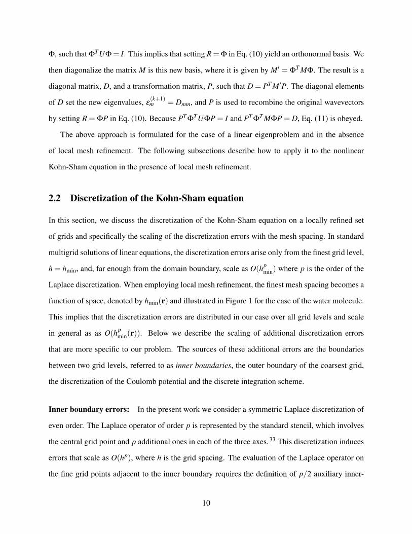
function of space, denoted by hmin(r) and illustrated in Figure 1 for the case of the water molecule.

This implies that the discretization errors are distributed in our case over all grid levels and scale

in general as as O(hpmin(r)). Below we describe the scaling of additional discretization errors

that are more specific to our problem. The sources of these additional errors are the boundaries

between two grid levels, referred to as inner boundaries, the outer boundary of the coarsest grid,

the discretization of the Coulomb potential and the discrete integration scheme.

Inner boundary errors: In the present work we consider a symmetric Laplace discretization of

even order. The Laplace operator of order p is represented by the standard stencil, which involves

the central grid point and p additional ones in each of the three axes.33 This discretization induces

errors that scale as O(hp), where h is the grid spacing. The evaluation of the Laplace operator on

the fine grid points adjacent to the inner boundary requires the definition of p/2 auxiliary inner-

10

10a0

Figure 1: Two-dimensional cross section of the grid hierarchy used for the initial approximation ofthe H2O molecule, presented on top of the electron density distribution, ρ(r). The solid lines rep-resent the inner-boundaries between two refinement patches. The coarsest mesh spacing depictedhere is h = 0.125a0, where a0 is the Bohr radius. The coarsest grid level used in the calculationhas a mesh spacing of h = 32a0 and extends over a cube, whose edge measures 800a0. The meshspacing of the finest grid level spanned around each atom is h = 2−14a0 ≈ 6.1 ·10−5a0.

11

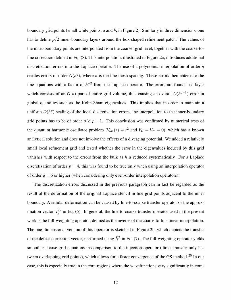
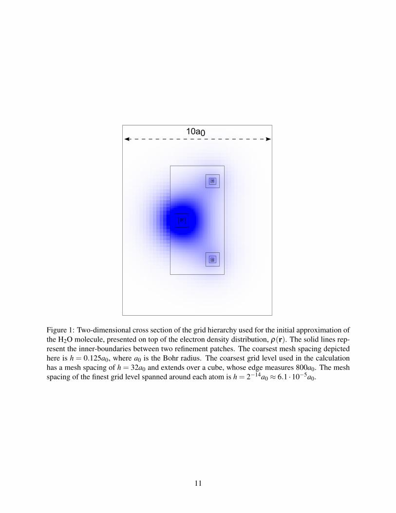
boundary grid points (small white points, a and b, in Figure 2). Similarly in three dimensions, one

has to define p/2 inner-boundary layers around the box-shaped refinement patch. The values of

the inner-boundary points are interpolated from the coarser grid level, together with the coarse-to-

fine correction defined in Eq. (8). This interpolation, illustrated in Figure 2a, introduces additional

discretization errors into the Laplace operator. The use of a polynomial interpolation of order q

creates errors of order O(hq), where h is the fine mesh spacing. These errors then enter into the

fine equations with a factor of h−2 from the Laplace operator. The errors are found in a layer

which consists of an O(h) part of entire grid volume, thus causing an overall O(hq−1) error in

global quantities such as the Kohn-Sham eigenvalues. This implies that in order to maintain a

uniform O(hp) scaling of the local discretization errors, the interpolation to the inner-boundary

grid points has to be of order q ≥ p+ 1. This conclusion was confirmed by numerical tests of

the quantum harmonic oscillator problem (Vion(r) = r2 and VH = Vxc = 0), which has a known

analytical solution and does not involve the effects of a diverging potential. We added a relatively

small local refinement grid and tested whether the error in the eigenvalues induced by this grid

vanishes with respect to the errors from the bulk as h is reduced systematically. For a Laplace

discretization of order p = 4, this was found to be true only when using an interpolation operator

of order q = 6 or higher (when considering only even-order interpolation operators).

The discretization errors discussed in the previous paragraph can in fact be regarded as the

result of the deformation of the original Laplace stencil in fine grid points adjacent to the inner

boundary. A similar deformation can be caused by fine-to-coarse transfer operator of the approx-

imation vector, I2hh in Eq. (5). In general, the fine-to-coarse transfer operator used in the present

work is the full-weighting operator, defined as the inverse of the coarse-to-fine linear interpolation.

The one-dimensional version of this operator is sketched in Figure 2b, which depicts the transfer

of the defect-correction vector, performed using I2hh in Eq. (7). The full-weighting operator yields

smoother coarse-grid equations in comparison to the injection operator (direct transfer only be-

tween overlapping grid points), which allows for a faster convergence of the GS method.20 In our

case, this is especially true in the core-regions where the wavefunctions vary significantly in com-

12

(b)

A B C D

a b c d e f

Coarse point Coarse point

with fine eq.

Fine

point Inner bound.

point

A B C D

a b c d e f

(c)

A B C D

a b c d e f

(a)

A B C D

a b c d e f

(d)

wc+wC

wBwA

g

g

g

g

h (x) = 2hmin h (x) = hmin

h (x) = 2hmin h (x) = hmin

h (x) = 2hmin h (x) = hmin

h (x) = 2hmin h (x) = hmin

E

E

E

E

wd we+wD wf wg

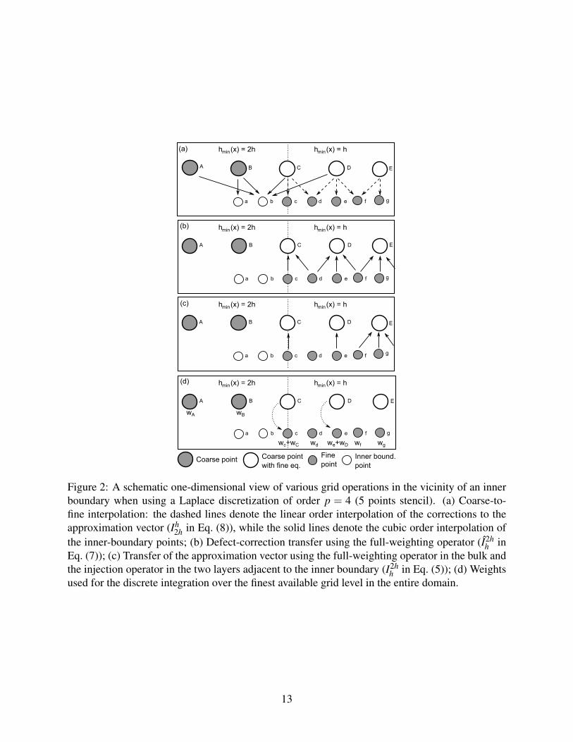
Figure 2: A schematic one-dimensional view of various grid operations in the vicinity of an innerboundary when using a Laplace discretization of order p = 4 (5 points stencil). (a) Coarse-to-fine interpolation: the dashed lines denote the linear order interpolation of the corrections to theapproximation vector (Ih

2h in Eq. (8)), while the solid lines denote the cubic order interpolation ofthe inner-boundary points; (b) Defect-correction transfer using the full-weighting operator (I2h

h inEq. (7)); (c) Transfer of the approximation vector using the full-weighting operator in the bulk andthe injection operator in the two layers adjacent to the inner boundary (I2h

h in Eq. (5)); (d) Weightsused for the discrete integration over the finest available grid level in the entire domain.

13

parison to the mesh spacing. However, using the full-weighting operator sketched in Figure 2b, for

the fine-to-coarse transfer of the approximation vector, defined in Eq. (5), induces discretization

errors in the coarse layers adjacent to the inner boundary (points A and B in Figure 2 for a Laplace

discretization of order p = 4). This is because the stencil describing the Laplace operator at points

A, B is then different from that of the standard stencil at grid level 2h. The resulting discretization

errors in the approximation vectors scale as O(h2). They enter into the coarse equations with an

h−2 factor from the Laplace operator in layers that comprise an O(h) part of the grid volume. The

resulting errors in the eigenvalues therefore scale as O(h), as confirmed by numerical tests. In

order to avoid this problem and achieve a uniform O(hp) scaling of the errors, the wavevectors

are transferred by injection from p layers of fine grid points adjacent to the inner boundary. This

modification is demonstrated by the injection from point c to C and from point e to D in Figure 2c

. Because the wavevectors are smooth in comparison with the mesh spacing close to the edge of

the refinement patch, the injection operator can be used there without harming the convergence of

the multigrid process.

Integration errors: Another source of discretization errors is the integration scheme employed

when evaluating global variables such as the elements of the Ritz matrix, Mi j, in Eq. (12). In

order to obtain the most accurate value, this integration is done using grid points that correspond to

finest available mesh spacing, hmin(r). We compute the integration weights associated with each

grid point by considering a polynomial interpolation of order q of a general vector, denoted by T,

which yields a continuous function, denoted by T (r). In order to integrate the finest mesh spacing,

the value at r is interpolated only from grid level hmin(r). By integrating T (r) over the entire space

we obtain a discrete sum over the elements of T, given by

∫d3rT (r) = ∑

iwiTi, (13)

where the resulting weights, wi, define the discrete integration scheme. The errors induced by

this scheme are due to the polynomial interpolation and hence scale as O(hq). Because wi are

14

calculated once and for all, upon setting the grid formation, q can be chosen to be higher than

that of the Laplace discretization, p, with negligible computational cost. We thus chose q = p+2.

Interpolating T (r) using grid level hmin(r) implies that several coarse grid points, close to the

inner boundary in the region spanned by the fine grid level (points C, D in Figure 2d), are also

assigned integration weights. In practice, we transfer their weights to the corresponding fine grid

points, as depicted by the arrows in Figure 2d. In principle, the same should have applied to the

inner-boundary grid points (a, b in Figure 2d), but this is avoided by obtaining T (r) in the fine

grid points adjacent to the inner boundary (points b,c and e) using an asymmetric polynomial

interpolation which involves only the fine grid points.

The above integration scheme, which uses the finest available mesh spacing, is denoted here

and below as ⟨ ⟩. In addition to it, we use a different integration scheme in order to compute

global variables during the V-cycle on a single grid level. The weights of this coarse integration

scheme on grid level h, denoted by ⟨ ⟩h, are obtained by adding weights from grid levels finer

than h to their corresponding coarse grid points using the full-weighting operator. In Figure 2d the

definition of ⟨ ⟩2h would imply that the weights of points c,d,e, f and g are added to points C,D

and E using the full-weighting operator illustrated in Figure 2b. This integration scheme does not

take into account, however, regions of space that are covered only by coarser grid levels. This issue

is solved by adding coarse correction to the integral, as discussed in Eq. (2.4).

Potential discretization errors: We conclude this section by discussing the discretizaion of the

Coulomb potential. The naive real-space discretization of the singular ionic potential, whereby

V hion,i =Vion(ri), provides a bad approximation of the continuous Kohn-Sham equation in the vicin-

ity of the nuclei and may lead to a very large condition number. We therefore use a smooth ap-

proximation of the Coulomb potential near the cores, obtained by averaging it over a cube around

each grid point. This potential is defined as

V ha (ri) =

1|ri| |ri|> c h

h−3 ∫ h2− h

2dx∫ h

2− h

2dy∫ h

2− h

2dz 1

|ri+x| else, (14)

15

where ri is the distance of the grid point from the position of the atom. The cutoff parameter

is chosen in our case to be c = 3. The cutoff assures that away from the singularity the Coulomb

potential is represented by its value at the location of each grid point, similarly to all other quantities

in the problem. The above integral can be evaluated analytically using the Gauss theorem, which

yields

∫ d3x|ri +x|

=12

∫ ri +x|ri +x|

· nd2x

= ∑x

∑p

xh/2

ξx

[ξy log(ξz + |ξ |)− ξx

2arctan(

ξyξz

ξx|ξ |)

], (15)

where ξ = ri +x , ∑x runs over the corners of the cube and ∑p denotes all permutations over the

x,y,z indices. The total ionic potential is given by a sum of Eq. (14) over all the atoms,

V hion,i = ∑

aZaV h

a (xi −Ra), (16)

where Za and Ra are the charges and positions of atoms, respectively. Numerical tests indicate that

this approximation of the true potential induces local discretization errors in the eigenvalues that

scale as O(h2) near the core. These errors, however, decrease sharply with the distance from the

core. We therefore reduce them by greatly refining small regions around the nuclei, as illustrated

in Figure 1. Since these additional refinement patches are small (cubic patches of size 173 grid

points), the computational cost of this solution is relatively small. The precise manner by which

the sizes and shapes of the refinement regions are determined is described in Section 2.5.

2.3 Relaxation Methods

In the present work, the Kohn-Sham equation, as well as the Poisson equation used for evaluat-

ing the Hartree potential, are computed using a more efficient generalization of the lexicographic

Gauss-Seidel method (4), known as the red-black Gauss Seidel (RBGS) method (see section 3.4

in Brandt20). In the RBGS method, the relaxation sweep is performed first over all grid points

16

with odd indices and then over all grid points with even indices (in d dimensions the sum of the d

indices should be odd or even, respectively). The RBGS relaxation sweeps converge for positive-

definite matrices such as the one corresponding to the Laplace discretization.34 The presence of

the Coulomb potential yields a small number of ‘binding’ eigenvectors with negative eigenvalue,

whereas most of the eigenvalues of the discrete operator remain positive. This slight non-positive-

definiteness causes smooth error components of the approximation vector, that are proportional to

the ‘binding’ eigenvectors, to diverge slowly when employing the RBGS method. However, on all

grid levels except for the coarsest one, this divergence is canceled by the coarse-grid corrections.

On the coarsest grid level, where we cannot rely on a yet coarser grid level, we employ instead

of the RBGS method the Kaczmarz method, which converges even for non-positive-definite op-

erators, albeit more slowly than RBGS.36 The key difference between the two methods is that in

each Kaczmarz iteration over a single grid point we alter the value of several neighbouring grid

points simultaneously. The properties of the Kaczmarz method and similar distributive methods

are further discussed in section 3.4 in Brandt20 and references therein. Because the role of the

coarsest grid level is in fact to solve the equation to very low residuals, as discussed below Eq.

(8), we employ in every V-cycle about 200 Kaczmarz relaxation sweeps on the coarsest grid, as

compared to only 4 RBGS sweeps on each of the finer grids.

The Coulomb potential causes a similar problem on finer grid levels in the vicinity of the

atoms, where the numerical values of the potential are comparable with the coefficient of the

Laplace discretization. As in the case of the coarsest grid level, this issue can be solved using the

Kaczmarz method. This is done by performing about 30 Kaczmarz relaxation sweeps on each fine

grid in cubic regions of size 73 grid points around the location of each atom, instead of the RBGS

relaxations. This region is increased during the relaxation to 113 grid points in order to prevent the

creation of high residuals on a single surface. This local relaxation is in accordance with the idea

of performing extra relaxation sweeps in regions that contain high residuals, proposed by Bai and

Brandt.37

It is worth noting that the amount of computer power invested in the large number of Kaczmarz

17

relaxation sweeps during each V -cycle is comparable to that invested in the RGBS relaxation

sweeps. This is because the overall number of grid points relaxed using the Kaczmarz method

is relatively small.

2.4 One-shot V-cycle of a nonlinear system

The Kohn-Sham equation is in fact a set of nonlinear equation. We first write down this set of

equations, while repeating for the sake of completeness several equations mentioned above, and

then discuss a self-consistent approach for solving them. The set of equations include the Kohn-

Sham equation of each orbital, defined as

(−∇2

2+Vion(r)+VH [ρ;r]+Vxc[ρ;r]

)φk(r) = εkφk(r), (17)

with a Dirichlet boundary condition, φk = 0, on the outer boundary of the domain. These equations

are nonlinear due to the dependence of the potentials on electron density. The definition of the

latter, presented also in Eq. (2), forms an additional equation in the set, given by

ρ(r) = ∑k

fk|φk(r)|2, (18)

where fk is the occupation number of wavevector k. The occupation numbers are set according to

the aufbau principle, i.e., from the lowest energy and up. Another equation is due to the conserva-

tion of charge, which implies that the wavevectors have to be normalized and hence

∫dr|φk(r)|2 = 1. (19)

The exchange-correlation potential in Eq. (17) is a functional of ρ and is defined as the functional

derivative of the exchange-correlation functional,

Vxc[ρ;r] =δ

δρExc[ρ]. (20)

18

In the present work, we implement the simplest approximation for Exc, known as the local den-

sity approximation (LDA), in which Vxc is taken to be a local function of ρ(r).38,39 The Hartree

potential is also a functional of ρ , obtained by solving the Poisson equation,

∇2VH =−4πρ(r), (21)

using the RBGS method. This Poisson equation has a nontrivial Dirichlet boundary condition on

the edge of the domain, which is approximated by a multipole expansion,40,41

VH(r,θ ,ϕ) =lmax

∑l=0

l

∑m=−l

4π2l +1

1rl+1Yl,m(θ ,ϕ)Qlm. (22)

Here Ylm are the spherical harmonic functions and the Qlm coefficients are given by

Qlm =∫

drdθdϕrlYl,m(θ ,ϕ)ρ(r,θ ,ϕ). (23)

In the present work we chose lmax = 9, which has been shown to provide sufficient precision by

comparing the results obtained in the present work to those obtained using a prolate-spheroidal

grid.16,17

Equations (17)-(23) form a set of nonlinear equations which can be solved using a self-consistency

cycle. A naive cycle would consist of solving Eq. (17) to very low residuals (through several V -

cycles), followed by an update of ρ , Vxc and the solution of Eq. (21), with ρ fixed, to very low

residuals. A great advantage of iterative solvers is that they allow one to perform a more effi-

cient self-consistency cycle whereby each equation is not solved to very low residuals in each

self-consistency step. Such an efficient cycle has been implemented within the DFT framework by

Kohn et al.,25 who recalculated the potentials after only a single V-cycle of Eq. (17). One can take

this idea one step further and update the potentials on each grid level after every relaxation sweep

on that level, following an approach known as the one-shot V-cycle.42 By creating high coupling

between the components of the nonlinear equation, the one-shot V-cycle is able to converge much

19

faster than the alternating cycle, where the potentials are updated only once per V-cycle after the

Rayleigh-Ritz process. We confirmed this by numerical tests for the hydrogen atom, where the

one-shot V-cycle was found to converge 5 to 10 times faster than the alternating cycle.

For linear equations and in the alternating cycle, the potentials in Eq. (17) are simply trans-

ferred to the coarse grid levels from the finest one by either the injection or the full-weighting

operator. In the one-shot V-cycle, however, the whole set of equations, (17)-(23), has to be trans-

ferred to the coarse grid levels according to the FAS scheme, described in Section 2.1.

The FAS scheme takes a slightly different form for an integral equation such as the normal-

ization condition, defined in Eq. (19). The latter has to be maintained during the one-shot V-cycle

because of the recalculation of the electron density according to Eq. (18), which is true only for

normalized Kohn-Sham orbitals. Because on all grid levels, excluding the finest, the Kohn-Sham

equation is in fact nonhomogeneous due to the fine-to-coarse defect correction, the normalization

of the wavevectors has to be accompanied by an update of the eigenvalues. The recalculation of

the eigenvalues can be done using the Rayleigh quotient formula,

εk =

∫drφ⋆

k (r)(−∇2

2 +Vion(r)+VH [ρ;r]+Vxc[ρ;r])

φk(r)∫dr|φk(r)|2

, (24)

which is obtained by integrating over Eq. (17).

Following the FAS scheme, we transfer the fine-grid corrections to the integrals in the above

equation and in Eq. (19). For a general integral over the entire domain,∫

drF(r), the fine-grid

corrections to level h are given by

τh/2,hF ≡ ⟨Fh/2⟩h/2 −⟨Ih

h/2Fh/2⟩h + τh/4,h/2F , (25)

where the inner-product is evaluated using the coarse integration scheme defined in Section 2.2, and

τh/4,h/2F denotes a similar correction transferred from grid level h/4 to grid level h/2. In addition,

we need to transfer a coarse-grid correction to∫

drF(r), that accounts for the contribution to the

integrals from regions of space that are covered only by grid levels that are coarser than h. This

20

correction is defined as

τ2h,hF ≡ ∑

i∈2hF2h

i wi + τ4h,2hF , (26)

where wi denotes the fine-integration weights. The weights for grid points on grid level 2h that

have corresponding grid points on grid level h (see Figure 2d). The correction from grid level 2h

also includes coarse-grid corrections from a yet coarser grid level, τ4h,2hF , which vanishes when

2h is the coarsest grid level. It is useful to note that the coarse-grid corrections vanish in standard

multigrid implementations (without local mesh refinement). Using these corrections the integral is

approximated on grid level h as,

∫drF(r)≈ ⟨Fh⟩h + τh/2,h

F + τ2h,hF . (27)

Following the above formulation, we can define the normalization factor, αhk , of the kth Kohn-

Sham orbital on grid level h as

(αhk )

2(⟨φh

k ,φhk⟩h + τ2h,h

φkφk

)+ τh/2,h

φkφk = 1, (28)

where τh/2,hφkφk and τ2h,h

φkφk are the fine-grid and coarse-grid corrections to the integral in Eq. (19),

respectively. This normalization factor is applied by setting

φh′k → αkφh′

k τh′,h′/2φkφk → α2

k τh′,h′/2φkφk (29)

on grid level h and all the coarser grid levels, h′ ≥ h. In order to save computational work the

actual multiplication of wavevectors on coarser levels is performed only upon entering each grid

level. Similarly, the eigenvalues are updated according to Eq. (24) as

εk =⟨φh

k ,Hhφh

k − τhk⟩h + τ2h,h

φkHφk+ τ

12 h,hφk(Hφk−τk)

⟨φhk ,φ

hk⟩h + τ2h,h

φkφk + τ12 h,hφkφk

, (30)

where τhk is the defect-correction vector of the Kohn-Sham equation, which is not to be confused

21

with the fine-grid and coarse-grid corrections to the numerator of Eq. (24), denoted by τh/2,hφk(Hφk−τk)

and τ2h,hφkHφk

, respectively. For a wavevector that has been normalized by the factor defined in Eq.

(28), the denominator in Eq. (30) is in fact equal to 1.

It is important to note that in usual applications of local mesh refinement we would need to en-

force global equations, such as the normalization of the wavevectors, only on very coarse grids that

span a significant portion of the domain. In our case, however, due to the singular potential, some

wavevectors are highly localized around the atoms. This implies that even grids that span a rela-

tively small volume around a single atom may still represent a significant portion of a wavevector

and thus require the relaxation to be accompanied by a normalization of the relevant wavevectors

and an update their eigenvalues.

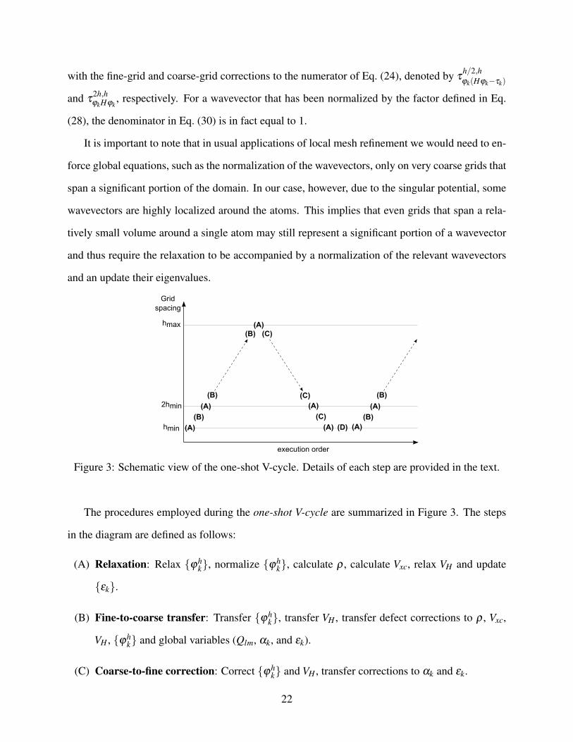
Figure 3: Schematic view of the one-shot V-cycle. Details of each step are provided in the text.

The procedures employed during the one-shot V-cycle are summarized in Figure 3. The steps

in the diagram are defined as follows:

(A) Relaxation: Relax {φhk}, normalize {φh

k}, calculate ρ , calculate Vxc, relax VH and update

{εk}.

(B) Fine-to-coarse transfer: Transfer {φhk}, transfer VH , transfer defect corrections to ρ , Vxc,

VH , {φhk} and global variables (Qlm, αk, and εk).

(C) Coarse-to-fine correction: Correct {φhk} and VH , transfer corrections to αk and εk.

22

(D) Rayleigh-Ritz process: Perform a modified Rayleigh-Ritz process (see Section 2.7) fol-

lowed by a recalculation of the coarse-to-fine corrections to αk and εk.

The one-shot V-cycle performs well for small systems such the hydrogen atom. However, in many

electron systems it was found to exhibit a very slow convergence of the residuals or even ill-

convergence in some of the cases. A careful study of the residuals suggested that the order of

operations on a single grid level, which alternates between relaxation sweeps of the Kohn-Sham

equation and updating of the potentials, did not provide enough coupling between the components

of the nonlinear set of equations. One approach to increase the coupling between components of

an ill-converging self-consistency cycle is through mixing of components from previous steps. In

this work we employ the generalized Broyden method43 which has been successfully implemented

in the past in electronic structure calculations.44,45 We used this method in order to yield a new

approximation of all the occupied wavevectors (for which fk = 0), Vxc, and VH , by mixing each

vector with its values from several previous relaxation sweeps. The weights of mixing are chosen

such that they minimize the overall residual of the Eqs. (17),(18) and (21). The mixing is used

only in combination with the Kaczmarz relaxation on the coarsest grid level and on finer ones in the

vicinity of the atoms, and hence its additional computational cost is relatively small. Mixing was

found to accelerate and sometimes enable the convergence of the many-electron systems discussed

in Section 3.

The effect of the mixing is presumably to reduce smooth components that diverge as a result

of the combination of relaxation sweeps and potential updates. The mixing algorithm is able to

single out these components from the difference between the current approximation vector and its

values in previous iterations, and reduce them from the current vector in a manner that minimizes

the overall residual of the set of nonlinear equation.

2.5 Grid refinement via a λ -FMG cycle

As with any self-consistent cycle, the one-shot V -cycle, described in Section 2.4, has to start from

an initial guess which is inside its basin of convergence. The multigrid approach provides an

23

inherent method for obtaining such an approximation, known as the Full Multigrid (FMG) al-

gorithm.20,21 We first describe the original algorithm, formulated within the standard multigrid

framework, where hmin is homogenous in space. The FMG cycle begins from a single coarse grid

or a small set of coarse grids where the initial approximation can be inexpensively obtained using

relatively costly methods such as a direct diagonalization of the discrete equations. Each FMG it-

eration consists of several V -cycles followed by an interpolation of the current approximation into

a new grid level whose mesh spacing is half of the currently finest mesh spacing, hmin → hmin/2.

These iterations are repeated until the discretization errors, whose estimation is discussed below,

have been reduced below a desired level. The generalization of this concept to the case of locally-

refined multigrids is known as the λ -FMG cycle (see section 9.6 in Brandt20). According to this

approach, every several V-cycles hmin(r) is refined in various regions of space, which can be auto-

matically chosen in a manner that yields a desired increase in accuracy using the minimal amount

of computational work.

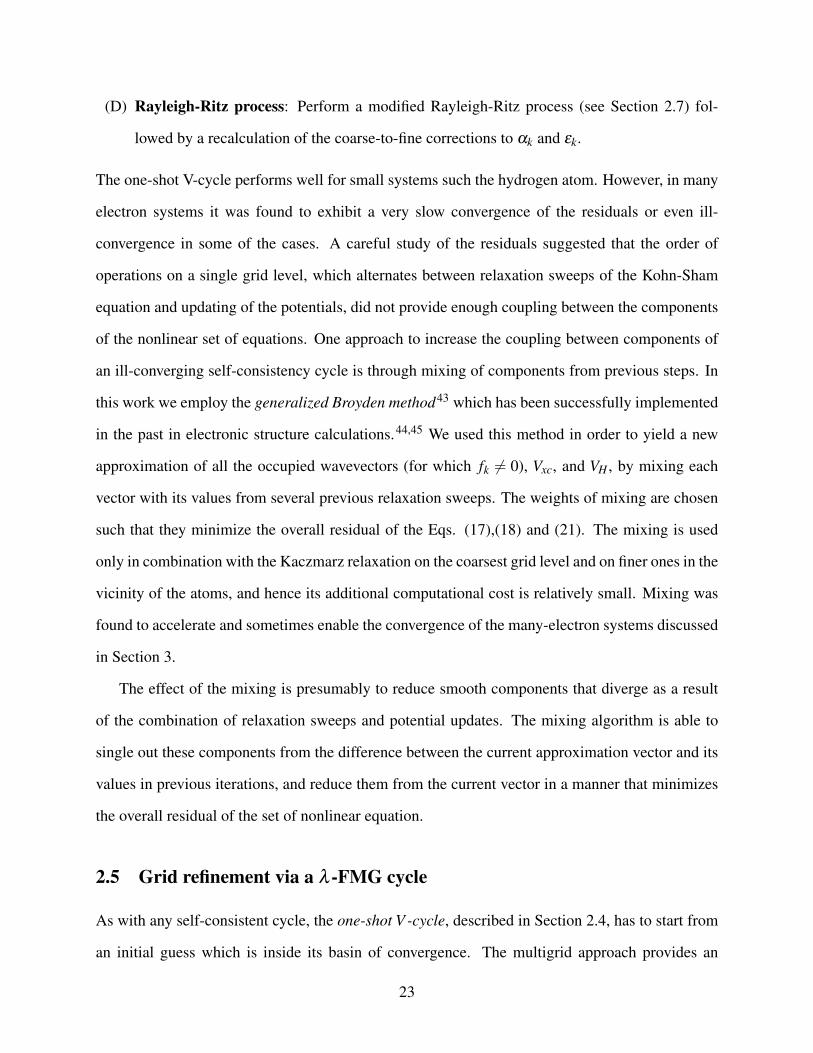
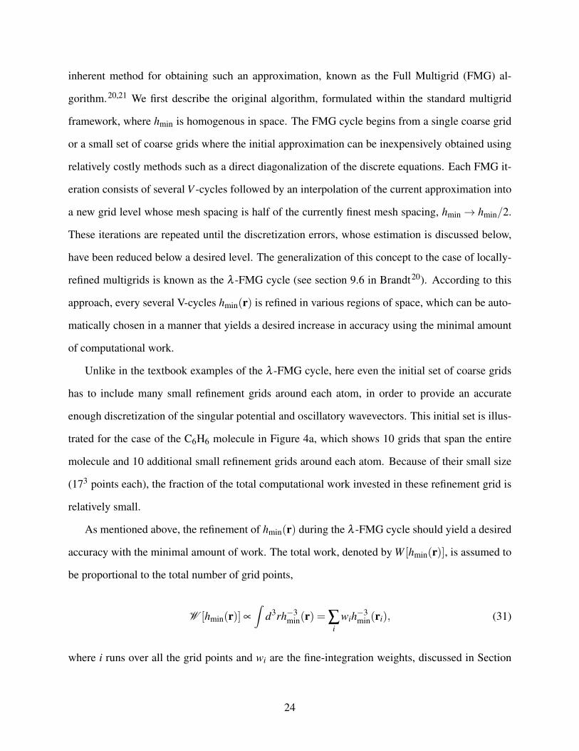
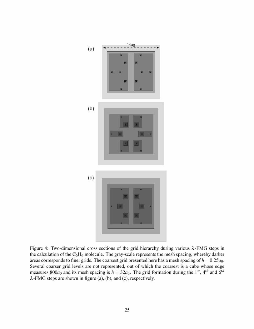
Unlike in the textbook examples of the λ -FMG cycle, here even the initial set of coarse grids

has to include many small refinement grids around each atom, in order to provide an accurate

enough discretization of the singular potential and oscillatory wavevectors. This initial set is illus-

trated for the case of the C6H6 molecule in Figure 4a, which shows 10 grids that span the entire

molecule and 10 additional small refinement grids around each atom. Because of their small size

(173 points each), the fraction of the total computational work invested in these refinement grid is

relatively small.

As mentioned above, the refinement of hmin(r) during the λ -FMG cycle should yield a desired

accuracy with the minimal amount of work. The total work, denoted by W [hmin(r)], is assumed to

be proportional to the total number of grid points,

W [hmin(r)] ∝∫

d3rh−3min(r) = ∑

iwih−3

min(ri), (31)

where i runs over all the grid points and wi are the fine-integration weights, discussed in Section

24

(a)

(b)

(c)

14a0

Figure 4: Two-dimensional cross sections of the grid hierarchy during various λ -FMG steps inthe calculation of the C6H6 molecule. The gray-scale represents the mesh spacing, whereby darkerareas corresponds to finer grids. The coarsest grid presented here has a mesh spacing of h= 0.25a0.Several coarser grid levels are not represented, out of which the coarsest is a cube whose edgemeasures 800a0 and its mesh spacing is h = 32a0. The grid formation during the 1st , 4th and 6th

λ -FMG steps are shown in figure (a), (b), and (c), respectively.

25

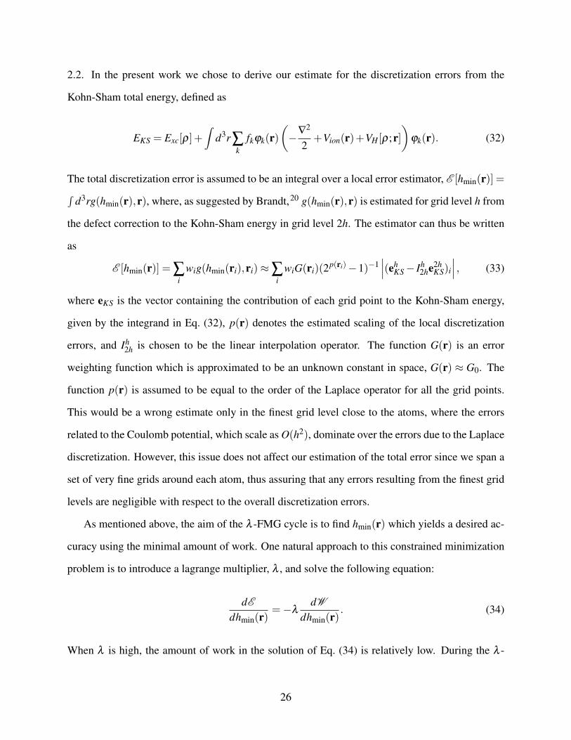
2.2. In the present work we chose to derive our estimate for the discretization errors from the

Kohn-Sham total energy, defined as

EKS = Exc[ρ]+∫

d3r∑k

fkφk(r)(−∇2

2+Vion(r)+VH [ρ;r]

)φk(r). (32)

The total discretization error is assumed to be an integral over a local error estimator, E [hmin(r)] =∫d3rg(hmin(r),r), where, as suggested by Brandt,20 g(hmin(r),r) is estimated for grid level h from

the defect correction to the Kohn-Sham energy in grid level 2h. The estimator can thus be written

as

E [hmin(r)] = ∑i

wig(hmin(ri),ri)≈ ∑i

wiG(ri)(2p(ri)−1)−1∣∣∣(eh

KS − Ih2he2h

KS)i

∣∣∣ , (33)

where eKS is the vector containing the contribution of each grid point to the Kohn-Sham energy,

given by the integrand in Eq. (32), p(r) denotes the estimated scaling of the local discretization

errors, and Ih2h is chosen to be the linear interpolation operator. The function G(r) is an error

weighting function which is approximated to be an unknown constant in space, G(r) ≈ G0. The

function p(r) is assumed to be equal to the order of the Laplace operator for all the grid points.

This would be a wrong estimate only in the finest grid level close to the atoms, where the errors

related to the Coulomb potential, which scale as O(h2), dominate over the errors due to the Laplace

discretization. However, this issue does not affect our estimation of the total error since we span a

set of very fine grids around each atom, thus assuring that any errors resulting from the finest grid

levels are negligible with respect to the overall discretization errors.

As mentioned above, the aim of the λ -FMG cycle is to find hmin(r) which yields a desired ac-

curacy using the minimal amount of work. One natural approach to this constrained minimization

problem is to introduce a lagrange multiplier, λ , and solve the following equation:

dE

dhmin(r)=−λ

dW

dhmin(r). (34)

When λ is high, the amount of work in the solution of Eq. (34) is relatively low. During the λ -

26

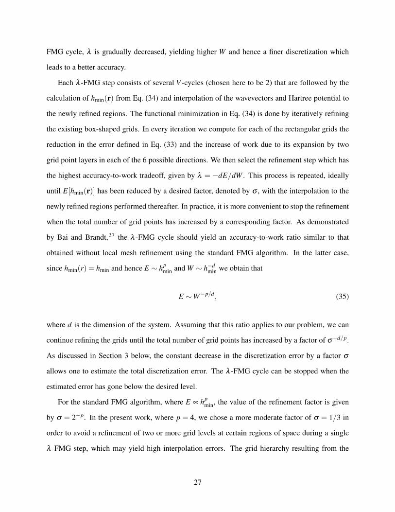
FMG cycle, λ is gradually decreased, yielding higher W and hence a finer discretization which

leads to a better accuracy.

Each λ -FMG step consists of several V -cycles (chosen here to be 2) that are followed by the

calculation of hmin(r) from Eq. (34) and interpolation of the wavevectors and Hartree potential to

the newly refined regions. The functional minimization in Eq. (34) is done by iteratively refining

the existing box-shaped grids. In every iteration we compute for each of the rectangular grids the

reduction in the error defined in Eq. (33) and the increase of work due to its expansion by two

grid point layers in each of the 6 possible directions. We then select the refinement step which has

the highest accuracy-to-work tradeoff, given by λ = −dE/dW . This process is repeated, ideally

until E[hmin(r)] has been reduced by a desired factor, denoted by σ , with the interpolation to the

newly refined regions performed thereafter. In practice, it is more convenient to stop the refinement

when the total number of grid points has increased by a corresponding factor. As demonstrated

by Bai and Brandt,37 the λ -FMG cycle should yield an accuracy-to-work ratio similar to that

obtained without local mesh refinement using the standard FMG algorithm. In the latter case,

since hmin(r) = hmin and hence E ∼ hpmin and W ∼ h−d

min we obtain that

E ∼W−p/d, (35)

where d is the dimension of the system. Assuming that this ratio applies to our problem, we can

continue refining the grids until the total number of grid points has increased by a factor of σ−d/p.

As discussed in Section 3 below, the constant decrease in the discretization error by a factor σ

allows one to estimate the total discretization error. The λ -FMG cycle can be stopped when the

estimated error has gone below the desired level.

For the standard FMG algorithm, where E ∝ hpmin, the value of the refinement factor is given

by σ = 2−p. In the present work, where p = 4, we chose a more moderate factor of σ = 1/3 in

order to avoid a refinement of two or more grid levels at certain regions of space during a single

λ -FMG step, which may yield high interpolation errors. The grid hierarchy resulting from the

27

above algorithm with σ = 1/3 is shown in Figure 4 for the case of the C6H6 molecule.

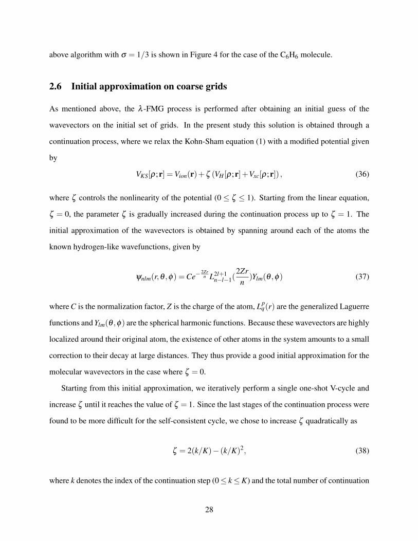
2.6 Initial approximation on coarse grids

As mentioned above, the λ -FMG process is performed after obtaining an initial guess of the

wavevectors on the initial set of grids. In the present study this solution is obtained through a

continuation process, where we relax the Kohn-Sham equation (1) with a modified potential given

by

VKS[ρ;r] =Vion(r)+ζ (VH [ρ;r]+Vxc[ρ;r]) , (36)

where ζ controls the nonlinearity of the potential (0 ≤ ζ ≤ 1). Starting from the linear equation,

ζ = 0, the parameter ζ is gradually increased during the continuation process up to ζ = 1. The

initial approximation of the wavevectors is obtained by spanning around each of the atoms the

known hydrogen-like wavefunctions, given by

ψnlm(r,θ ,ϕ) =Ce−2Zr

n L2l+1n−l−1(

2Zrn

)Ylm(θ ,ϕ) (37)

where C is the normalization factor, Z is the charge of the atom, Lpq(r) are the generalized Laguerre

functions and Ylm(θ ,ϕ) are the spherical harmonic functions. Because these wavevectors are highly

localized around their original atom, the existence of other atoms in the system amounts to a small

correction to their decay at large distances. They thus provide a good initial approximation for the

molecular wavevectors in the case where ζ = 0.

Starting from this initial approximation, we iteratively perform a single one-shot V-cycle and

increase ζ until it reaches the value of ζ = 1. Since the last stages of the continuation process were

found to be more difficult for the self-consistent cycle, we chose to increase ζ quadratically as

ζ = 2(k/K)− (k/K)2, (38)

where k denotes the index of the continuation step (0≤ k ≤K) and the total number of continuation

28

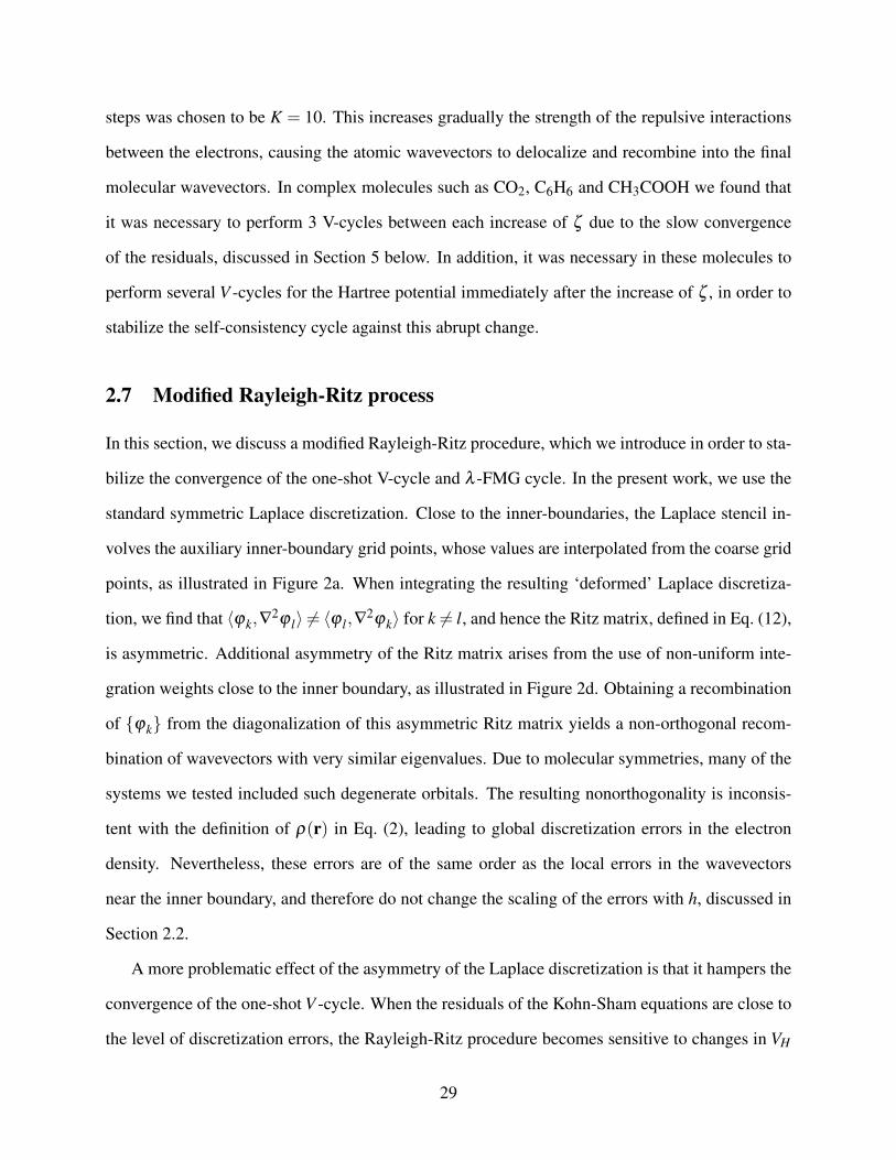
steps was chosen to be K = 10. This increases gradually the strength of the repulsive interactions

between the electrons, causing the atomic wavevectors to delocalize and recombine into the final

molecular wavevectors. In complex molecules such as CO2, C6H6 and CH3COOH we found that

it was necessary to perform 3 V-cycles between each increase of ζ due to the slow convergence

of the residuals, discussed in Section 5 below. In addition, it was necessary in these molecules to

perform several V -cycles for the Hartree potential immediately after the increase of ζ , in order to

stabilize the self-consistency cycle against this abrupt change.

2.7 Modified Rayleigh-Ritz process

In this section, we discuss a modified Rayleigh-Ritz procedure, which we introduce in order to sta-

bilize the convergence of the one-shot V-cycle and λ -FMG cycle. In the present work, we use the

standard symmetric Laplace discretization. Close to the inner-boundaries, the Laplace stencil in-

volves the auxiliary inner-boundary grid points, whose values are interpolated from the coarse grid

points, as illustrated in Figure 2a. When integrating the resulting ‘deformed’ Laplace discretiza-

tion, we find that ⟨φk,∇2φ l⟩ = ⟨φ l,∇2φk⟩ for k = l, and hence the Ritz matrix, defined in Eq. (12),

is asymmetric. Additional asymmetry of the Ritz matrix arises from the use of non-uniform inte-

gration weights close to the inner boundary, as illustrated in Figure 2d. Obtaining a recombination

of {φk} from the diagonalization of this asymmetric Ritz matrix yields a non-orthogonal recom-

bination of wavevectors with very similar eigenvalues. Due to molecular symmetries, many of the

systems we tested included such degenerate orbitals. The resulting nonorthogonality is inconsis-

tent with the definition of ρ(r) in Eq. (2), leading to global discretization errors in the electron

density. Nevertheless, these errors are of the same order as the local errors in the wavevectors

near the inner boundary, and therefore do not change the scaling of the errors with h, discussed in

Section 2.2.

A more problematic effect of the asymmetry of the Laplace discretization is that it hampers the

convergence of the one-shot V -cycle. When the residuals of the Kohn-Sham equations are close to

the level of discretization errors, the Rayleigh-Ritz procedure becomes sensitive to changes in VH

29

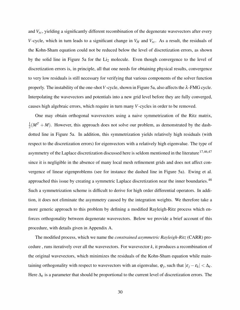
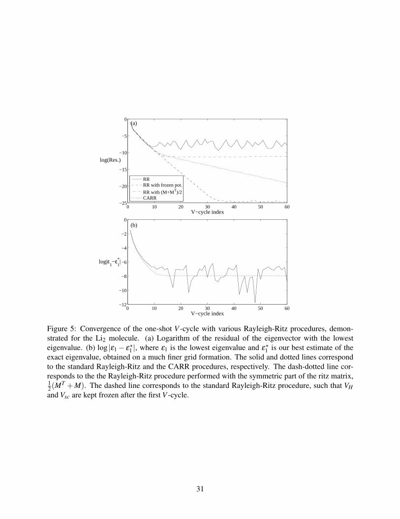
and Vxc, yielding a significantly different recombination of the degenerate wavevectors after every

V -cycle, which in turn leads to a significant change in VH and Vxc. As a result, the residuals of

the Kohn-Sham equation could not be reduced below the level of discretization errors, as shown

by the solid line in Figure 5a for the Li2 molecule. Even though convergence to the level of

discretization errors is, in principle, all that one needs for obtaining physical results, convergence

to very low residuals is still necessary for verifying that various components of the solver function

properly. The instability of the one-shot V -cycle, shown in Figure 5a, also affects the λ -FMG cycle.

Interpolating the wavevectors and potentials into a new grid level before they are fully converged,

causes high algebraic errors, which require in turn many V -cycles in order to be removed.

One may obtain orthogonal wavevectors using a naive symmetrization of the Ritz matrix,

12(M

T +M). However, this approach does not solve our problem, as demonstrated by the dash-

dotted line in Figure 5a. In addition, this symmetrization yields relatively high residuals (with

respect to the discretization errors) for eigenvectors with a relatively high eigenvalue. The type of

asymmetry of the Laplace discretization discussed here is seldom mentioned in the literature17,46,47

since it is negligible in the absence of many local mesh refinement grids and does not affect con-

vergence of linear eigenproblems (see for instance the dashed line in Figure 5a). Ewing et al.

approached this issue by creating a symmetric Laplace discretization near the inner boundaries.48

Such a symmetrization scheme is difficult to derive for high order differential operators. In addi-

tion, it does not eliminate the asymmetry caused by the integration weights. We therefore take a

more generic approach to this problem by defining a modified Rayleigh-Ritz process which en-

forces orthogonality between degenerate wavevectors. Below we provide a brief account of this

procedure, with details given in Appendix A.

The modified process, which we name the constrained asymmetric Rayleigh-Ritz (CARR) pro-

cedure , runs iteratively over all the wavevectors. For wavevector k, it produces a recombination of

the original wavevectors, which minimizes the residuals of the Kohn-Sham equation while main-

taining orthogonality with respect to wavevectors with an eigenvalue, φ j, such that |ε j − εk|< ∆ε .

Here ∆ε is a parameter that should be proportional to the current level of discretization errors. The

30

0 10 20 30 40 50 60−25

−20

−15

−10

−5

0

V−cycle index

log(Res.)

0 10 20 30 40 50 60−12

−10

−8

−6

−4

−2

0

V−cycle index

log|ε1−ε

1* |

RRRR with frozen pot.

RR with (M+MT)/2CARR

(a)

(b)

Figure 5: Convergence of the one-shot V -cycle with various Rayleigh-Ritz procedures, demon-strated for the Li2 molecule. (a) Logarithm of the residual of the eigenvector with the lowesteigenvalue. (b) log |ε1 − ε⋆1 |, where ε1 is the lowest eigenvalue and ε⋆1 is our best estimate of theexact eigenvalue, obtained on a much finer grid formation. The solid and dotted lines correspondto the standard Rayleigh-Ritz and the CARR procedures, respectively. The dash-dotted line cor-responds to the the Rayleigh-Ritz procedure performed with the symmetric part of the ritz matrix,12(M

T +M). The dashed line corresponds to the standard Rayleigh-Ritz procedure, such that VHand Vxc are kept frozen after the first V -cycle.

31

result is a transformation that minimizes the residuals while maintaining a high level of orthog-

onality between degenerate wavevectors (nonorthogonality is kept much lower than the level of

discretization errors). As a result, the recombination of the degenerate wavevectors is not sensitive

to changes in VH and Vxc, leading to a stable convergence of the residuals, as demonstrated by the

dotted line in Figure 5a. Figure Figure 5b shows the difference between the eigenvalue of the low-

est eigenvector and its more precise value obtained on a finer grid settings. The figure demonstrates

that the CARR procedure does not change the precision in comparison to the usual Rayleigh-Ritz

procedure.

We emphasize strongly that one can consider various generalizations of the CARR process that

may make it more efficient than the standard Rayleigh-Ritz process and that may prove essential

to overall scaling of our approach. This is discussed further in Appendix A

3 Numerical Results

In this section, we present numerical results obtained using the above approach, implemented in a

program we named CARMA (Concurrent All-electron Real-space Multigrid Algorithm). We first

discuss the method used for estimating the discretization errors and analyze its performance in

detail for the case of the H2 molecule. We then present high accuracy results for several molecular

systems and compare them to corresponding values found in the literature and to results obtained

from calculations based on gaussian basis sets.

Before presenting the results obtained for various molecules, we provide some additional in-

formation about the practical implementation of the approach discussed in the previous sections.

Exchange-correlation functional : All calculations were performed for the spin-unpolarized

Kohn-Sham equation using the local density approximation (LDA) exchange-correlation energy

functional, in the parameterized form given by Perdew and Wang.39

32

Transfer operators : The Kohn-Sham and Hartree equations were represented using a 4th order

Laplace discretization. As explained in Section 2.2, this requires a discrete integration operator

which is based on a 6th order polynomial interpolation and a 6th order interpolation of the inner-

boundary grid points (sketched in Figure 2a). The same order of interpolation is required when

refining the {φk} and VH during the λ -FMG cycle. In general, fine-to-coarse transfers (operators

I2hh and I2h

h in Eqs. (5), (7), and (8)) were performed using the full-weighting operator sketched in

Figure 2b. As discussed in Section 2.2, {φk} and VH need to be transferred via injection to grid

points close to the inner boundary in order to avoid inducing additional discretization errors (see

Figure 2c). Coarse-to-fine corrections (operator Ih2h in Eq. (8)) were transferred using the linear

interpolation operator.

Grid structure: In all computations, the coarsest grid had a mesh spacing of h = 32a0 and

spanned a cubic region around the molecule whose edge measured 800a0. By comparison to pre-

vious calculations of diatomic molecules, this choice can be shown to yield sufficiently negligible

outer-boundary discretization errors. The approach of local mesh refinement allows this distance to

be further increased with negligible computational cost, by expanding the coarsest grid or adding

a coarser grid level. The initial grid formation included also 5-8 finer grids that spanned the entire

molecule and a set of small refinement grids around each atom, such that the finest mesh spacing

was h = 2−15a0 ≃ 1.6 ·10−15m. The geometries of the molecules are given in Table Table 1.

λ -FMG cycle: The results presented below were obtained using the λ -FMG algorithm described

in Section 2.5. One important parameter in this algorithm is σ , which is taken to be σ = 1/3 in

order to prevent the possibility of double grid refinement in a single λ -FMG step (this option is

also excluded in the implementation of the algorithm). The number of V-cycles performed in every

λ -FMG step was chosen to be 2. In choosing this number we had to consider the fact that during

each one-shot V-cycle the residuals were reduced by a factor that varied between 2 to 5. This

convergence rate is slow with respect to standard multigrid implementations, as further discussed

in Section 5. This suggests, that in order order to maintain the residual below the level of the

33

discretization errors (which decrease with the rate σ = 1/3) one has to perform at least 2 V-cycles

between every λ -FMG step.

A crucial feature in any numerical approach is a reliable estimate of the discretization errors. In

our case we estimate the error by measuring the difference in total energy between two consecutive

λ -FMG steps. Assuming that the error drops by a constant factor, σ , during every λ -FMG step

(see Section 2.5), one can estimate the discretization error to be

E f ≈∣∣∣( f (i)− f (i−1))/(σ−1

f −1)∣∣∣ , (39)

where f (i) is the value of a global function, e.g. the total energy, and σ f is the factor by which

the discretization error drops in every λ -FMG step. The (i) superscript denotes here and below

a quantity which is evaluated at the end of the ith λ -FMG step. In the case where f = EKS we

expect that σEKS = σ , where σ is the factor used in the definition of the λ -FMG cycle. For other

quantities, σ f can be estimated as

σ f ≈∣∣∣( f (i)− f (i−1))/( f (i−1)− f (i−2))

∣∣∣ . (40)

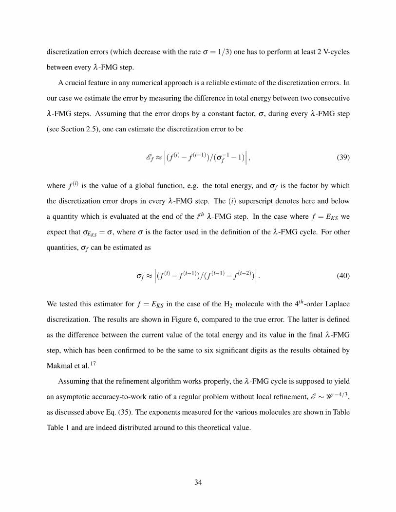
We tested this estimator for f = EKS in the case of the H2 molecule with the 4th-order Laplace

discretization. The results are shown in Figure 6, compared to the true error. The latter is defined

as the difference between the current value of the total energy and its value in the final λ -FMG

step, which has been confirmed to be the same to six significant digits as the results obtained by

Makmal et al.17

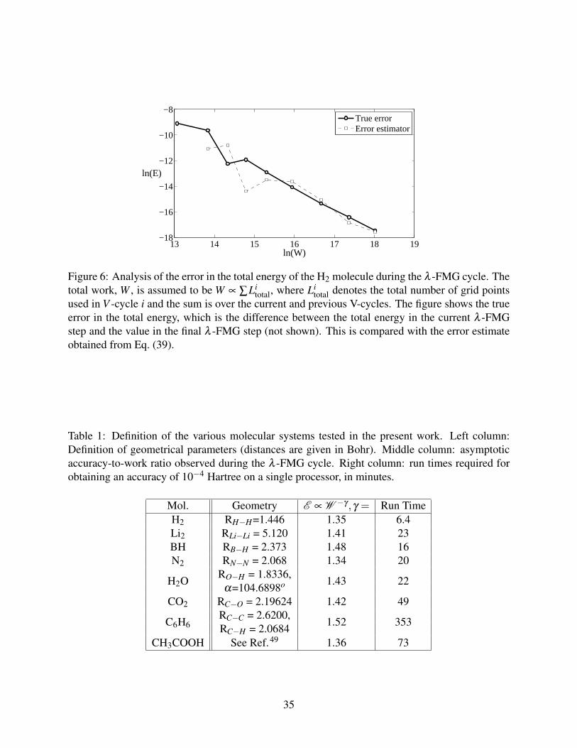
Assuming that the refinement algorithm works properly, the λ -FMG cycle is supposed to yield

an asymptotic accuracy-to-work ratio of a regular problem without local refinement, E ∼ W −4/3,

as discussed above Eq. (35). The exponents measured for the various molecules are shown in Table

Table 1 and are indeed distributed around to this theoretical value.

34

13 14 15 16 17 18 19−18

−16

−14

−12

−10

−8

ln(W)

ln(E)

True errorError estimator

Figure 6: Analysis of the error in the total energy of the H2 molecule during the λ -FMG cycle. Thetotal work, W , is assumed to be W ∝ ∑Li

total, where Litotal denotes the total number of grid points

used in V -cycle i and the sum is over the current and previous V-cycles. The figure shows the trueerror in the total energy, which is the difference between the total energy in the current λ -FMGstep and the value in the final λ -FMG step (not shown). This is compared with the error estimateobtained from Eq. (39).

Table 1: Definition of the various molecular systems tested in the present work. Left column:Definition of geometrical parameters (distances are given in Bohr). Middle column: asymptoticaccuracy-to-work ratio observed during the λ -FMG cycle. Right column: run times required forobtaining an accuracy of 10−4 Hartree on a single processor, in minutes.

Mol. Geometry E ∝ W −γ ,γ = Run TimeH2 RH−H=1.446 1.35 6.4Li2 RLi−Li = 5.120 1.41 23BH RB−H = 2.373 1.48 16N2 RN−N = 2.068 1.34 20

H2ORO−H = 1.8336,

1.43 22α=104.6898o

CO2 RC−O = 2.19624 1.42 49

C6H6RC−C = 2.6200,

1.52 353RC−H = 2.0684

CH3COOH See Ref.49 1.36 73

35

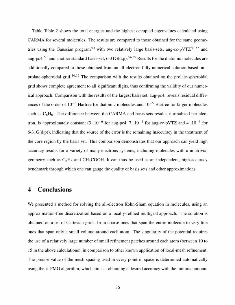
Table Table 2 shows the total energies and the highest occupied eigenvalues calculated using

CARMA for several molecules. The results are compared to those obtained for the same geome-

tries using the Gaussian program50 with two relatively large basis-sets, aug-cc-pVTZ51,52 and

aug-pc4,53 and another standard basis-set, 6-31G(d,p).54,55 Results for the diatomic molecules are

additionally compared to those obtained from an all-electron fully numerical solution based on a

prolate-spheroidal grid.16,17 The comparison with the results obtained on the prolate-spheroidal

grid shows complete agreement to all significant digits, thus confirming the validity of our numer-

ical approach. Comparison with the results of the largest basis set, aug-pc4, reveals residual differ-

ences of the order of 10−6 Hartree for diatomic molecules and 10−5 Hartree for larger molecules

such as C6H6. The difference between the CARMA and basis sets results, normalized per elec-

tron, is approximately constant (3 · 10−6 for aug-pc4, 7 · 10−4 for aug-cc-pVTZ and 4 · 10−3 for

6-31G(d,p)), indicating that the source of the error is the remaining inaccuracy in the treatment of

the core region by the basis set. This comparison demonstrates that our approach can yield high

accuracy results for a variety of many-electrons systems, including molecules with a nontrivial

geometry such as C6H6 and CH3COOH. It can thus be used as an independent, high-accuracy

benchmark through which one can gauge the quality of basis sets and other approximations.

4 Conclusions

We presented a method for solving the all-electron Kohn-Sham equation in molecules, using an

approximation-free discretization based on a locally-refined multigrid approach. The solution is

obtained on a set of Cartesian grids, from coarse ones that span the entire molecule to very fine

ones that span only a small volume around each atom. The singularity of the potential requires

the use of a relatively large number of small refinement patches around each atom (between 10 to

15 in the above calculations), in comparison to other known application of local-mesh refinement.

The precise value of the mesh spacing used in every point in space is determined automatically

using the λ -FMG algorithm, which aims at obtaining a desired accuracy with the minimal amount

36

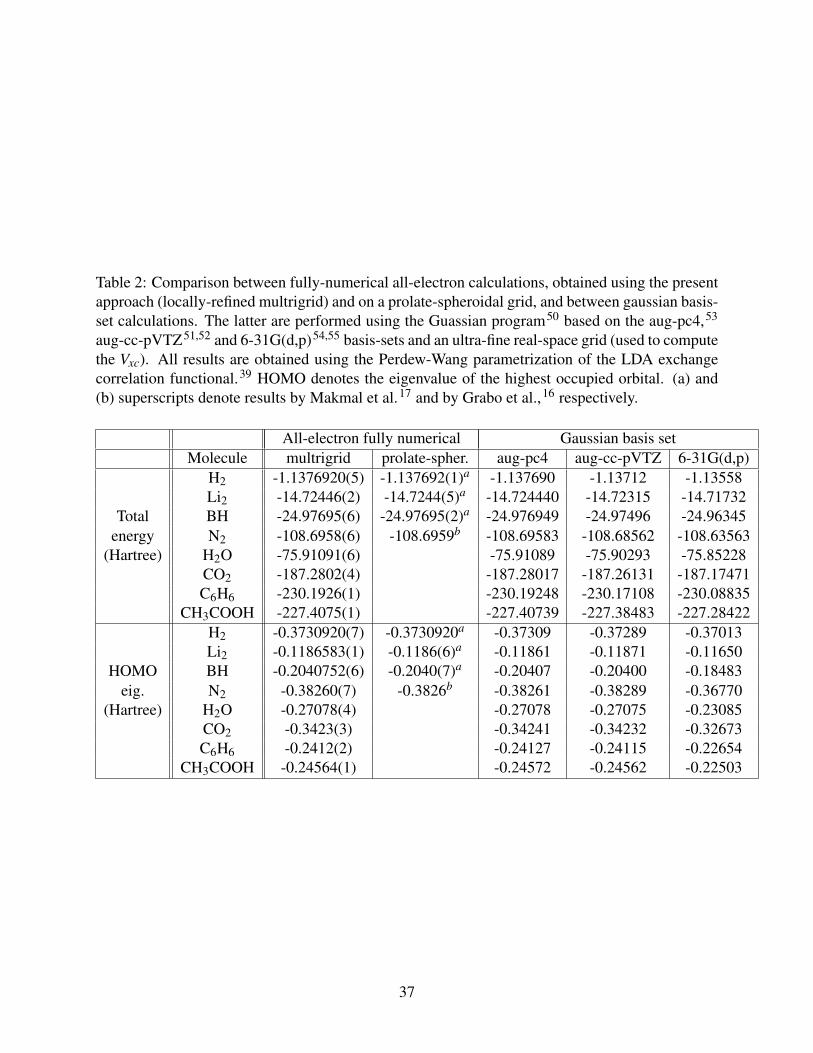
Table 2: Comparison between fully-numerical all-electron calculations, obtained using the presentapproach (locally-refined multrigrid) and on a prolate-spheroidal grid, and between gaussian basis-set calculations. The latter are performed using the Guassian program50 based on the aug-pc4,53

aug-cc-pVTZ51,52 and 6-31G(d,p)54,55 basis-sets and an ultra-fine real-space grid (used to computethe Vxc). All results are obtained using the Perdew-Wang parametrization of the LDA exchangecorrelation functional.39 HOMO denotes the eigenvalue of the highest occupied orbital. (a) and(b) superscripts denote results by Makmal et al.17 and by Grabo et al.,16 respectively.

All-electron fully numerical Gaussian basis setMolecule multrigrid prolate-spher. aug-pc4 aug-cc-pVTZ 6-31G(d,p)

H2 -1.1376920(5) -1.137692(1)a -1.137690 -1.13712 -1.13558Li2 -14.72446(2) -14.7244(5)a -14.724440 -14.72315 -14.71732

Total BH -24.97695(6) -24.97695(2)a -24.976949 -24.97496 -24.96345energy N2 -108.6958(6) -108.6959b -108.69583 -108.68562 -108.63563

(Hartree) H2O -75.91091(6) -75.91089 -75.90293 -75.85228CO2 -187.2802(4) -187.28017 -187.26131 -187.17471C6H6 -230.1926(1) -230.19248 -230.17108 -230.08835

CH3COOH -227.4075(1) -227.40739 -227.38483 -227.28422H2 -0.3730920(7) -0.3730920a -0.37309 -0.37289 -0.37013Li2 -0.1186583(1) -0.1186(6)a -0.11861 -0.11871 -0.11650

HOMO BH -0.2040752(6) -0.2040(7)a -0.20407 -0.20400 -0.18483eig. N2 -0.38260(7) -0.3826b -0.38261 -0.38289 -0.36770

(Hartree) H2O -0.27078(4) -0.27078 -0.27075 -0.23085CO2 -0.3423(3) -0.34241 -0.34232 -0.32673C6H6 -0.2412(2) -0.24127 -0.24115 -0.22654

CH3COOH -0.24564(1) -0.24572 -0.24562 -0.22503

37

of computational work. This algorithm allows us to solve the Kohn-Sham equation with an accu-

racy to work tradeoff which is similar to that of obtained in simple discretizations of nonsingular

problems.

While the standard multigrid approach is often demonstrated for linear and regular equations,

here the combination of a nonlinear eigenproblem and a singular potential requires advanced multi-

grid techniques, described in detailed in Section 2. Specifically, in order to accelerate the conver-

gence of the residuals of the nonlinear set of equations, their self-consistent solution is obtained

using a one-shot V-cycle, whereby the whole set is solved on each grid level during the V-cycle.

The boundaries between the large number of refinement patches yield a significantly asymmetric

Laplace discretization, which may destabilize this self-consistency cycle. To overcome this prob-

lem we introduce a modified Rayleigh-Ritz procedure. This procedure may be necessary in the

future to accelerate the self-consistency cycle and achieve a linear scaling of the computational

power with the number of atoms in the molecule.

The results obtained using the above approach agree to all significant digits with previous

all-electron calculation of diatomic molecules, where the Kohn-Sham equation was solved on a

prolate-spheroidal grid.16,17 For more complex molecules, namely H2O, CO2, CH3COOH and

C6H6, our results show very good agreement with gaussian basis set calculations, up to a level

which appears to correspond to the accuracy limit of the basis set approximation. For the purposes

of this article, all results were obtained using a simple exchange-correlation energy functional,

namely the LDA one, with a fixed geometry of the molecule. Nevertheless, the above approach

is readily applicable to more advanced physical scenarios. In the next and final section, we point

out various avenues for further improvement and refinement of our approach. In particular, we

describe a slow convergence phenomenon of the residuals of Kohn-Sham equation for relatively

high eigenvalues and suggest that it may be removed using inter-grid interpolation operators that

are adapted to the oscillatory form of the wavevectors.

38

5 Future perspective

In this section, we discuss possible extensions of the above approach. The interested reader may

also wish to consider a general survey of research directions in multigrid implementations of DFT,

found in section 9 of Brandt.42

Our approach is readily applicable to more elaborate physical scenarios, one of which is the use

of orbital-dependent exchange-correlation energy functionals.7 The use of such functionals within

the Kohn-Sham scheme requires the additional solution of an integro-differential equation known

as the optimized effective potential (OEP) equation.7 In the OEP approach, the self-consistent cal-

culation of the exchange-correlation potential consumes a significant portion of the computational

work. As demonstrated above for the case of the Hartree potential, using the one-shot V-cycle

to compute this exchange-correlation potential may accelerate its convergence in comparison to

similar non-multigrid implementations.

Other interesting physical features that can be incorporated in this approach are geometrical

optimization and periodic boundary conditions. The λ -FMG cycle provides a natural framework

for an efficient geometrical optimization process, whereby the coarse relocations of the atoms are

performed during the initial stages of the cycle on a set of coarse grids, during which the calculation

of the forces is less demanding. The grid structure implemented in this study also provides an

efficient way of modifying the wavevectors upon a relocation of an atom. The small refinement

grids should move with the atom they enclose, requiring little change to their wavevectors. On the

other hand, the coarse grids that remain static may require several additional relaxation steps or

a W -cycle20 to account for the change in the geometry of the molecule. Because the grid points

in the finest ‘static’ grid level and the coarsest ‘movable’ grid level may not overlap exactly, this

would require employing grid transfer operators between two nonoverlapping grid levels.

In the present implementation of the above approach, all the wavevectors are represented on

all the grid levels. Our algorithm can be made more efficient by not representing wavevectors that

are localized around certain atoms on local-refinement grids that are spanned around other atoms.

As a result, the necessary computational work and memory storage would scale linearly with the

39

number of electrons in the molecule, rather than as the number of electrons times the number of

atoms. The efficiency can be further increased by keeping fine-to-coarse defect corrections of very

fine grid levels frozen during some of the V-cycles, as suggested in section 15 in Brandt.20 Further

improvement in efficiency can be obtained by allowing refinement grids to overlap. In CARMA,

when the λ -FMG algorithm causes two refinement grids to expand into the same region they are

united into a single larger refinement grid, as demonstrated in Figure 4. Allowing refinement grids

to overlap can reduce the number of grid points required for solving complex molecules such

as C6H6. Such overlap may also be necessary in order to obtain optimal parallelization of the

algorithm.

One possible extension of the mixing scheme discussed in Section 2.4, which was crucial for

the convergence of the one-shot V-cycle, would be to mix between the approximation vectors

in previous V -cycles and to incorporate this type of mixing also in the Rayleigh-Ritz procedure.

Another possible approach to this issue is to perform a simultaneous relaxation of Eqs. (17),

(18),(20), and (21) instead of the usual Kaczmarz relaxation. This idea is known in the multigrid

methodology as collective relaxation (see section 3.4 in Brandt20). In order to implement it, one

would have to expand the set of equations to linear order in terms of small changes in {φk}, VH and

Vxc. Each collective Kaczmarz iteration should then consist of diagonalizing the resulting matrix

and altering together all the occupied wavevectors, VH , and Vxc, at a certain grid point and at its

nearest neighbours.

In Appendix A we discuss several possible extensions of the Constrained Asymmetric Rayleigh

Ritz (CARR) process, introduced in Section 2.7, that may increase the efficiency of the V -cycle.

One possible direction is to perform the CARR procedure on coarse grids. Another idea is to

accelerate the convergence of the self-consistency cycle, by taking into account small changes in

the potential while computing the optimal recombination of the wavevectors. In addition, one may

consider recombining the wavevectors with their values in previous V-cycles. This amounts to

using the multigrid cycle as a preconditionner for the conjugate gradient algorithm. This idea has

yielded significant increase in the efficiency of various multigrid implementations in other fields,

40

as discussed in section 7.3 of Brandt.20

The approach presented above did not attain the textbook V -cycle convergence rates. During

a single ‘healthy’ V-cycle the residuals of the equations that being solved should drop by a factor

of about 10.20 The typical factors found using CARMA varied between 3 to 6 in simple systems

such as H2 or Li2. Oscillatory wavevectors appeared to converge more slowly than the smooth

ones, causing many-electron systems such as CO2 or C6H6, where such oscillatory wavevectors

are occupied, to converge even more slowly at a rate of about 2. Because we have observed this

issue also in the linear case (in high eigenvectors of the hydrogen atom, where Vion = 1/r and

Vxc = VH = 0), we may exclude nonlinear effects as a possible explanation for this phenomenon.

In addition, the absence of this issue in the harmonic case (Vion = r2 and Vxc = VH = 0), suggests

that the polynomial based grid transfer operators might not provide a good coarse description of the

oscillatory wavevectors in the proximity of the cores. If this is indeed the source of the problem, it

may be solved by constructing optimal interpolation operators, following the approach of the exact

interpolation scheme (EIS).56,57 Another possible direction is to use local refinement grids that are

based on spherical coordinates, where the angular behavior of the wavevectors in the vicinity of

the cores is regular. The EIS should also be more efficient on spherical refinement grids, where

one should only fit the radial dependence of the interpolation operators to the structure of the

wavevectors.

Acknowledgement

We thank A. Biller, A. Makmal, A. Natan, and L. Segev for helpful discussions. We further thank

J. M. L. Martin for expert advice on gaussian basis-set issues. This work was supported by the

European Research Council and the Lise Meitner Minerva Center for Computational Chemistry.

41

A Constrained Asymmetric Rayleigh Ritz (CARR) process

In this appendix, we present a modified Rayleigh-Ritz procedure, which we name the Constrained

Asymmetric Rayleigh Ritz (CARR) process. The original purpose of the CARR process is to find

an optimal recombination of the wavevectors at the end of each V -cycle, that would minimize

the residual of the Kohn-Sham equation, per each wavevector, while maintaining orthogonality

between degenerate wavevectors. The CARR process allows the one-shot V -cycle, presented in

Section 2.4, to converge smoothly to very low residuals, well below the level of discretization

errors. Such convergence, although not necessary for obtaining additional physical precision, was

needed in order to verify that all the components of the solver function properly. In addition, the

CARR process has several advantages, discussed below, which may be crucial for studying larger

molecular systems and for using orbital-dependent exchange-correlation energy functionals.

The starting point of the CARR algorithm is the original set of wavevector, {φk}, and eigen-

values, {εk}, where k = 1, . . . ,N. The algorithm iteratively seeks a set of new eigenvalues, {ε ′k},

and a recombination matrix, bk j, which defines a new set of wavevectors via φ ′k = ∑N

j=1 bk jφ j.

Each wavevector, {φ ′k}, should minimize the residual of its Kohn-Sham equation while remain-

ing normalized and orthogonal to eigenvectors with a similar eigenvalue. These conditions can be

translated to the following set of equations over bk and ε ′k:

Mkbk = εkbk bTk Ubl = δkl ∀l : |εk − εl| ≤ ∆ε (41)

where ∆ε is an energy cutoff, whose value is discussed below, and

(Mk)i j ≡ ⟨φhi ,H

hk φh

j⟩, Ui j ≡ ⟨φhi ,φ

hj⟩. (42)

The above inner products are evaluated throughout space on the finest available grid using the in-

tegration weights described in Section 2.2. The k subscript of M and H imply that the Hamiltonian

may in fact be discretized differently for each wavevector or contain an orbital-dependent poten-

42

tial, as found in some advance approximations of Vxc.7 Allowing for such orbital-dependence is an

important advantage of the CARR process over the standard Rayleight-Ritz process.

Equation (41) can be linearized by assuming small changes in bk and in εk, which yields an

iterative solution given by

(Mk − ε(t)k I

)b(t+1)

k −b(t)k ε(t+1)

k =−ε(t)k b(t)k (43)

(1+δkl)b(t+1),Tk Ub(t)

l = δkl +b(t),Tk Ub(t)

l . (44)

Here b(t)k ,ε(t)k denote the approximation of the eigenvector and eigenvalue at the t’th iteration,

respectively. The number of eigenvalues obeying |εk − εl| ≤ ∆ε is denoted, here on, as Nk∆, and

their indices are given as (k, i1, . . . , iNk∆−1). In this notation, Eq. (43) can be written as a set of

N +Nk∆ linear equations given by

ε(t)k I −Mk b(t)k b(t)

i1 . . .

2b(t),Tk U 0 0

b(t),Ti1 U 0 0

... . . .

b(t),TiNk

∆−1U 0 0

b(t+1)k U

ε(t+1)k

µ1

...

µiNk

∆−1

=

ε(t)k b(t)k

1+ |b(t)k Ub(t)

k |

0...

0

, (45)

where µ is a vector of ghost parameters. One drawback of this approach is that, unlike the stan-

dard Rayleigh-Ritz process, it relies on an initial guess for the eigenvectors and eigenvalues. A

natural choice which often works is to use the identity matrix, b(0) = I, and set also ε(0)i = εi.

However, during the continuation process, where the wavevectors and potentials may undergo sig-

nificant changes between every V -cycle, it is necessary to start the process by diagonalizing first

the symmetrized Ritz matrix, 12(M+MT ). The diagonalization yields a diagonal matrix, D, and a

transformation matrix, P, such that D = PT 12(M+MT )′P. The starting point of the CARR process

should in this case be b(0) = P and ε(0)i = Dii.

The value of ∆ε has to be chosen carefully in order to suit the current level of discretization

43

error. When ∆ε is taken to be too large, the CARR process cannot separate vector components

with different eigenvalues as needed for minimizing the residuals (see explanation below Eq. (10)),

leading in turn to very slow convergence rates. On the other hand, when ∆ε is too small the CARR

process may yield the same transformation matrix, b, as the one obtained using by the standard

Rayleigh-Ritz procedure. In this case, as discussed in Section 2.7, the residuals cannot converge

below the level of discretization errors.

In general the CARR process converges very quickly, and in most cases it reaches its fixed

point after no more than 5 iterations. We found, however, that the process converges very slowly,

or even diverges, if it involves wavevectors with positive eigenvalues. These wavevectors are not

localized around the atom and their convergence is not important for the calculation of steady-state

electronic structure. In order to avoid the convergence problem we simply excluded them from the

CARR process.

One may consider several extensions to the CARR process in order to improve the efficiency

of the one-shot V -cycle. One possible extension is to perform the CARR procedure not only on the

finest grid level, but on several coarse grid levels. This would require transferring fine corrections

to the Mk and U matrices, defined in Eq. (41), using Eq. (25), as well as using the right hand side

of the coarse Kohn-Sham equations.

The standard Rayleigh-Ritz process, as well as the CARR process described above, require

integrating N2 inner products over space. For complex molecules which consist of many eigen-

vectors, this integration requires a significant amount of computational work. In order to increase

the efficiency of this evaluation, the wavevectors should be separated into partially-overlapping

subspaces, each of which includes wavevectors with a common physical property such as being

located around a certain atom. The CARR process should then be performed within each sub-

space, while alternating between between the subspaces. The computer power required for such

an implementation would scale as O(N), instead of O(N2).

Another possible extension of the CARR process is to take into account small changes in the

Hartree and exchange-correlation potentials when seeking for the optimal recombination of the

44

wavevector. In order to formulate the resulting procedure, we first examine the change in the

electron density due to a small change in the eigenvector k, which is given by

δρ(k)(x) =N

∑i=1

(1+δki)(bk, i −δki) fkφi(x)φk(x), (46)

where fk is the orbital occupation-number. The resulting change in the potentials is given by

δV (k)xc (x) =

δVxc

δρ

∣∣∣∣ρ(x)

δρ(k)(x), (47)

δV (k)H (x) =

N

∑i=1

fk(1+δki)(bk, i −δki)bk,iUk,i(x), (48)

where Uk,i are the solutions of the Poisson equation

∇2Uk,i(x) =−4πφk(x)φi(x). (49)

These terms can then be incorporated in the iterative form of Eq. (43), yielding

(Mk +δM(1)

k − ε(t)k I)

b(t+1)k −b(t)

k ε(t+1)k = (δM(2)

k − ε(t)k )b(t)k (50)

where the addition to matrix in the LHS is given by

(δM(1)k )i j = 2

∫dxφi(x)

[∑l,m

(b(t)l,m −δlm) fmRlm(x)φ j(x)+∑m

fkb(t)k,mφm(x)Rk j(x)

], (51)

with

Rlm(x) =δVxc

δρ

∣∣∣∣ρ(x)

φl(x)φm(x)+Ul,m(x). (52)

The additional matrix in the RHS of Eq. (50) is given by

(δM(2)k )i j = 2

∫dxφi(x)φ j(x) fkRkk(x). (53)

45

Here the sum over m and l runs from 1 to N and the integral over x is evaluated using the fine

integration scheme, presented in Section 2.2.

Performing this kind of recombination should in principle add a significant computational cost

to the one-shot V-cycle, especially due to the solution of the N2 Poisson equation defined in Eq.

(49). However, because Uk,i are relatively smooth (similarly to the Hartree potential), they need be

computed only on relatively coarse grid levels. In this way, the work invested in the solution of

Eq. (49) would be comparable to that invested in the computation of the Hartree potential over the

entire grid formation. This approach may also useful for the evaluation of certain orbital-dependent

exchange-correlations functional that depend on Uk,i as well.

References

(1) Parr, R. G.; Yang, W. Density-functional theory of atoms and molecules; Oxford university

press, 1989; Vol. 16.

(2) Gross, E. K.; Dreizler, R. M. Density functional theory; Plenum Publishing Corporation,

1995; Vol. 337.

(3) Pickett, W. E. Comput. Phys. Rep. 1989, 9, 115 – 197.

(4) Chelikowsky, J. R.; Cohen, M. L. Handbook on Semiconductors 1992, 1, 59.

(5) Cramer, C. J. Essentials Of Computational Chemistry; John Wiley and Sons, New York,

2002; p 166.

(6) Hirata, S.; Ivanov, S.; Grabowski, I.; Bartlett, R.; Burke, K.; Talman, J. D. J. Chem. Phys.

2001, 115, 1635.

(7) Kümmel, S.; Kronik, L. Rev. Mod. Phys. 2008, 80, 3.

(8) Gómez-Abalo, R.; Li, X.; Scheffler, M.; Ambrosch-Draxl, C. Phys. Rev. Lett. 2008, 101,

106404.

46

(9) Pask, J.; Sterne, P. Modelling and Simulation in Materials Science and Engineering 2005, 13,

R71.

(10) Fattebert, J. L.; Hornung, R. D.; Wissink, A. M. J. Com. Phys. 2007, 223, 759–773.

(11) Bylaska, E. J.; Holst, M.; Weare, J. H. J. Chem. Theory Comput. 2009, 5, 937–948.

(12) Fang, J.; Gao, X.; Zhou, A. J. Comput. Phys. 2012, 231, 3166–3180.

(13) Bao, G.; Hu, G.; Liu, D. J. Comput. Phys. 2012.

(14) Lehtovaara, L.; Havu, V.; Puska, M. The Journal of chemical physics 2009, 131, 054103.

(15) Schauer, V.; Linder, C. J. Comput. Phys. 2013.

(16) Grabo, T.; Kreibich, T.; Gross, E. K. U. Molecular Engineering 1997, 7, 27–50.

(17) Makmal, A.; Kümmel, S.; Kronik, L. J. Chem. Theory Comput. 2009, 5, 1731–1740.

(18) Modine, N. A.; Zumbach, G.; Kaxiras, E. Phys. Rev. B 1997, 55, 10289.

(19) Beck, T. L. Rev. Mod. Phys. 2000, 72, 1041–1080.

(20) Brandt, A.; Livne, O. E. Multigrid Techniques - 1984 Guide with Applications to Fluid Dy-

namics (Revised Edition); SIAM, Philadelphia, PA, 2011.

(21) Briggs, W. L.; Emden, H. V.; McCormick, S. F. A Multigrid Tutorial, 2nd ed.; SIAM,

Philadelphia, PA, 2000.

(22) Trottenberg, U.; Oosterlee, C.; Schuller, A. Multigrid; Academic Press, New York, 2000.

(23) Brandt, A. Mathematics of Computation, American Mathematical Society 1977, 31, 333–390.

(24) Frehse, J.; Pallaschke, D.; Trottenberg, U. Special Topics in Applied Mathematics 1980, 31,

91–128.

47

(25) Kohn, S.; Weare, J.; Ong, E.; Baden, S. 8. SIAM conference on parallel processing for scien-

tific computing; 1996.

(26) Venkatesh, P. K. Physica B 2001, 318, 121–139.

(27) Saarikoski, H.; Räsänen, E.; Siljamäki, S.; Harju, A.; Puska, M.; Nieminen, R. The European

Physical Journal B-Condensed Matter and Complex Systems 2002, 26, 241–252.

(28) Feng, G.; Beck, T. L. Phys. Stat. Sol. (b) 2006, 243, 1054–1062.

(29) Wijesekera, N. R.; Feng, G.; Beck, T. L. Phys. Rev. B 2007, 75, 115101.

(30) Bernholc, J.; Hodak, M.; Lu, W. J. Phys.: Condens. Matter 2008, 20, 294205.

(31) Shimojo, F.; Kalia, R. K.; Nakano, A.; Vashishta, P. Phys. Rev. B 2008, 77, 085103.

(32) Beck, T. L. Intern. J. of Quan. Chem. 1998, 65, 477–486.

(33) Forenbrg, B.; Sloan, D. M. Acta Numerica 1994, 3, 203–267.

(34) Brandt, A. Applied Mathematics and Computation 1986, 19, 23–56.

(35) Brandt, A.; McCormick, S.; Ruge, J. SIAM J. Sci. Stat. Comput. 1983, 4, 244–260.

(36) Kaczmarz, S. Bulletin International de l’Academie Polonaise des Sciences et des Lettres

1937, A 35, 335–337.

(37) Bai, D.; Brandt, A. SIAM J. Sci. Stat. Comput. 1987, 8, 109–134.

(38) Perdew, J.; Zunger, A. Phys. Rev. B 1981, 23, 5048–5079.

(39) Perdew, J. P.; Wang, Y. Phys. Rev. B 1992, 45, 13244, In Gaussian this parametrization is

used by adding the keyword "SPW91 IOp(3/78=0000010000)".

(40) Landau, L. D.; Lifshitz, E. M. The Classical Theory of Fields, 4th ed.; Pergamon, Oxford,

1975; pp 97–99.

48

(41) Burdick, W. R.; Saad, Y.; Kronik, L.; Vasiliev, I.; Jain, M.; Chelikowsky, J. R. Computer

Physics Communications 2003, 156, 22 – 42.

(42) Brandt, A. In Multiscale Scientific Computation: Review 2001; T Barth, R. H., Chan, T., Eds.;

Springer Verlag, 2001.

(43) Eyert, V. J. Compu. Phys. 1996, 124, 271–285.

(44) Jain, M.; Kronik, L.; Chelikowsky, J. R.; Godlevsky, V. V. Phys. Rev. B 2001, 64, 245205.

(45) Remediakis, I. N.; Kaxiras, E.; Chen, M.; Friend, C. M. J. Chem. Phys. 2003, 118, 6046.

(46) Kohn, S.; Ong, J. H. W. E. M. G.; Baden, S. B. In Software and computational issues in

parallel structured adaptive mesh methods for electronic structure.

(47) Griebel, M.; Zumbusch, G. In Hash Based Adaptive Parallel Multilevel Methods with Space-

Filling Curves; Rollnik, H., Wolf, D., Eds.; John von Neumann Institut für Computing,

Forschungszentrum Jülich Germany, 2002; Vol. 9, pp 479–492.

(48) Ewing, R. E.; Lazarov, R. D.; Vassilevski, A. T. SIAM J. on Numer. Anal. 1990, 31, 1605–

1622.

(49) Nuclei coordinates in Bohr radii: C(0,0,0) , O(0,0,1.207217), O(1.14105,0,-0.716555), C(-

1.198642,-0.001044,-0.875179), H(1.869007,0.000356,-0.056682), H(-1.184665,0.882417,-

1.532696), H(-1.183545,-0.884834,-1.532234), H(-2.106195,-0.001464,-0.260919).

(50) Frisch, M. J. et al. Gaussian 03; Gaussian, Inc.: Wallingford, CT, 2004.

(51) Kendall, R. A.; Dunning Jr, T. H.; Harrison, R. J. J. Chem. Phys. 1992, 96, 6796.

(52) Woon, D. E.; Dunning Jr, T. H. J. Chem. Phys. 1993, 98, 1358.

(53) Jensen, F. Theor. Chem. Acc. 2005, 113, 187–190.

(54) Hehre, W. J.; Ditchfield, R.; Pople, J. A. J. Chem. Phys. 1972, 56, 2257.

49

(55) Francl, M. M.; Pietro, W. J.; Hehre, W. J.; Binkley, J. S.; Gordon, M. S.; DeFrees, D. J.;

Pople, J. A. J. Chem. Phys. 1982, 77, 3654–3665.

(56) Kushnir, D.; Galun, M.; Brandt, A. IEEE Trans. Pattern Anal. Mach. Intell. 2010, 32, 1377.

(57) Brandt, A.; Brannick, J.; Kahl, K.; Livshits, I. SIAM J. Sci. Comput. 2011, 33, 612–632.

50