Embed Size (px)
Citation preview

LOEWNER’S THEORY:A PARAMETRIC METHOD TO TACKLE PROBLEMS IN COMPLEX
ANALYSIS
MANUEL D. CONTRERAS
DEPARTAMENTO DE MATEMATICA APLICADA II AND IMUSUNIVERSIDAD DE SEVILLA
Contents
Introduction 20.1. Notation 31. The Bieberbach Conjecture 31.1. The area theorem and the case n = 2 41.2. An application of the case n = 2: Classical distortion theorems 62. Loewner Theory and the coefficient a3 92.1. First steps in Loewner theory 92.2. From Loewner chains to Loewner PDE and the case n = 3 in Bieberbach
conjecture 123. Loewner Theory and univalence criteria 153.1. From Loewner PDE to Loewner chains: evolution families 153.2. Univalence criteria 183.3. Recapitulation 204. An important example: the slit case 215. Chordal Loewner Theory 236. Prerequisites 266.1. Some results about Riemann mappings and convergence of domains 266.2. Distortion results for functions with non-negative real parts 296.3. Convergence of analytic functions 31References 32
Date: February 8, 2013.Key words and phrases. Loewner theory.These notes have been written for the introductory course Loewner Theory for the school “Doc-course
Complex Analysis and Related Areas” held in the Universities of Sevilla and Malaga, from February 4thtill March 15th, 2013.
1
2 M.D. CONTRERAS
Introduction
In 1923 K. Loewner introduced a new method in order to attack the famous Bieber-bach conjecture about Taylor coefficient estimates for univalent functions. Since then hismethod, known now as Parametric Representation of univalent functions, has been devel-oped by a number of prominent analysts, among which we have to mention fundamentalcontributions of P.P. Kufarev and Chr. Pommerenke. The Parametric RepresentationMethod, being a key ingredient in the proof of Bieberbach’s conjecture, given by L. deBrange in 1984, has however gone far beyond the scope of the initial problem. Two spectac-ular examples of its applications in other areas of Mathematics are the Loewner-Kufarevtype equation describing free boundary flow of a viscous fluid in a Hele-Shaw cell; and thehighly celebrated Stochastic Loewner Evolution (SLE) introduced in 2000 by O. Schrammas a powerful tool that led to deep results in the mathematical theory of some 2D latticemodels of great importance for Statistical Physics.
Originally, Loewner Theory was developed for univalent functions normalized at aninternal point of the reference domain. This case is referred nowadays to as the radialLoewner Evolution. The first paper on Parametric Method for functions normalized ata boundary point was probably published in 1949 by N.V. Popova, a student of P.P.Kufarev. This variant of the theory, marked in the modern terminology by the attributechordal, was developed by P.P. Kufarev, I.A. Aleksandrov, V.V. Sobolev, V.V. Goryainovand others. However, the importance of the chordal variant of Loewner Theory remainedunderestimated until O. Schramm, who used it to define SLE.
Another mathematical construction closely related to Loewner Theory is one-parametricsemigroups of holomorphic functions. This construction provides a set of important non-trivial examples for Operator Theory.
Classical Loewner theory can be consulted in the books by Conway [16], Duren [19], orPommerenke [33] meanwhile the state of the art of the general Loewner theory appearsin the surveys [2] and [9]. In these last papers a number of applications can be found.
Recently, in a series of papers by F. Bracci, S. Dıaz-Madrigal, P. Gumenyuk, andthe author, it was introduced a new unifying approach in Loewner Theory containingradial and chordal variants as special cases as well as one-parametric semigroups as anautonomous reduction. According to this approach the essence of Loewner Theory can berepresented via connection and interaction of three classes of objects:
• Time-dependent Herglotz vector fields in the unit disk, which generate non-autonomous holomorphic flows in the unit disk.• Evolution families, which can be characterized as systems of holomorphic endo-
morphisms of the unit disk generated by the above mentioned flows.• Loewner chains, which are one-parametric families of univalent functions with
expanding systems of image domains.
Any Loewner chain satisfies a linear PDE driven by a Herglotz vector field, and thecorresponding evolution family arises by solving the characteristic equation for this PDE.
LOEWNER’S THEORY 3
In this mini-course we will introduce the three main notions of the theory (Loewnerchains, Loewner differential equations, and evolution families), study their relationshipsand some applications like the proofs of the Bieberbach conjecture for the firsts Taylorcoefficients of a univalent function. We will discuss only the deterministic case.
These notes are written for people who have followed a previous course in ComplexAnalysis. In Section 6, we have collected a list of results we will use in the rest of thesections. The reader who is familiar with results about univalent functions can go directlyto the section about the Bieberbach conjecture.
0.1. Notation. D is the unit disk. For all a ∈ C and 0 < r < +∞, we define D(a, r) =z ∈ C : |z−a| < r and C(a, r) = z ∈ C : |z−a| = r. We denote by D∗ the punctureddisk, that is, D∗ := z ∈ C : 0 < |z| < 1.
1. The Bieberbach Conjecture
By S we denote the class of all univalent (i. e. holomorphic and injective) functionsf : D→ C normalized by
(1.1) f(z) = z ++∞∑n=2
anzn, z ∈ D := z ∈ C : |z| < 1.
In 1916, Ludwig Bieberbach posed his celebrated conjecture. This conjecture states thatif f belongs to S, then |an| ≤ n for each n. Bieberbach was able to prove the result forn = 2. In fact, this result is equivalent to the famous Koebe’s 1
4-theorem (see Subsection
1.1 for a detailed exposition).In 1923, Charles Loewner introduced a parametric method to tackle the general case
and proved the case n = 3. This method is nowadays known as Loewner theory and wasreally remarkable that Loewner ideas were also a key ingredient in the sophisticated proofof Bieberbach conjecture by de Branges in 1985. In this notes we will analyze the casesn = 2 and n = 3. For a complete proof the reader can see the book by Conway [16] whereit is presented a detailed exposition of the proof given by FitzGerald and Pommerenke[20].
Example 1.1 (The Koebe function). Consider f : D→ C given by
f(z) =z
(1− z)2=
1
4
[(1 + z
1− z
)2
− 1
].
Then f ∈ S, f(D) = C \ (−∞,−1/4] and f(z) =∑∞
n=1 nzn. In particular, f gives exactly
the bounds for the Bieberbach conjecture. Taking λ ∈ ∂D, we define Kλ(z) = λf(λz).Notice that Kλ ∈ S.

4 M.D. CONTRERAS
1.1. The area theorem and the case n = 2. To simplify the exposition we denote byU the class of all univalent functions g : D∗ → C with a simple pole at 0 and normalizedby
g(z) =1
z+ b0 + b1z + b2z
2 + ...
Theorem 1.2 (Area Theorem). For all g ∈ U ,
area(E) = π
[1−
∞∑m=1
m|bm|2],
where E = C \ g(D∗). In particular,
(1.2)∞∑m=1
m|bm|2 ≤ 1.
In these notes, we will only use the inequality (1.2). So we will prove only such inequality.With some additional work, the reader can get the value of area(E).
Proof. Given 0 < r < 1, we write Γr := g(C(0, r)). Since g is univalent, Γr is a smoothJordan curve. We denote by Ωr the unique bounded connected component of C \ Γr.Since g is univalent and limz→0 g(z) = ∞, we have that g(r < |z| < 1) ⊂ Ωr andg(0 < |z| < r) ⊂ C \ Ωr. Moreover, for r small enough, g(reiθ)) ≈ 1
re−iθ + b0 and then
0 ∈ Ωr.Take the parametrization of Γr given by γr : [0, 2π] → C with γr(θ) := g(re−iθ). We
claim that γr induces a positive orientation of Γr. To see this fact we argue as follows.Let us fix r0 < 1 and w0 = g(r0). Notice that w0 ∈ Ωr for all r < r0. As usual, I(Γ, z0)
stands for the index of the point z0 with respect to the Jordan curve Γ. The functionh(z) = zg(z) is holomorphic in the unit disk and h(0) = 1. In particular, for z smallenough h(z) 6= 0. Therefore, there is δ such that for 0 < r ≤ δ,
I(Γr, 0) =1
2πi
∫Γr
1
wdw =
1
2πi
∫C(0,r)−
g′(z)
g(z)dz
=1
2πi
∫C(0,r)−
(−1
z+h′(z)
h(z)
)dz = − 1
2πi
∫C(0,r)−
1
zdz = 1.
The invariance of the index under homotopy implies that
I(Γr, w0) = I(Γδ, w0) = I(Γδ, 0) = 1.
This proves the claim.Now we apply Green Theorem to calculate the area of Ωr:
area(Ωr) =
∫ ∫Ωr
1dxdy =1
2
∫Γ+r
xdy − ydx.

LOEWNER’S THEORY 5
Writing u(θ) := Re g(re−iθ) and v(θ) := Im g(re−iθ) we have
area(Ωr) =1
2
∫ 2π
0
(u(θ)v′(θ)− v(θ)u′(θ))dθ
=1
2
∫ 2π
0
(Re g(re−iθ)Im (−ire−iθg′(re−iθ))− Im g(re−iθ)Re (−ire−iθg′(re−iθ))
)dθ
= −1
2
∫ 2π
0
Re[g(re−iθ)re−iθg′(re−iθ)
]dθ
= −1
2Re
∫ 2π
0
g(re−iθ)re−iθg′(re−iθ)dθ.
Let us calculate the integrand
g(re−iθ)re−iθg′(re−iθ) =
(1
reiθ +
∞∑n=0
bnrne−inθ
)re−iθ
(− 1
r2e2iθ +
∞∑n=1
nbnrn−1e−i(n−1)θ
)
=
(1
reiθ +
∞∑n=0
bnrne−inθ
)(−1
re−iθ +
∞∑n=1
nbnrneinθ
)
= − 1
r2+∞∑n=1
nbnrn−1ei(n+1)θ −
∞∑n=0
bnrn−1e−i(n+1)θ +
+∞∑n=0
∞∑m=1
bnmbmrr+mei(m−n)θ.
Since∫ 2π
0eikθdθ = 0 for k 6= 0 and
∫ 2π
0ei0θdθ = 2π we have
0 ≤ area(Ωr) = −1
2
(− 1
r22π +
∞∑n=1
n|bn|2r2n2π
)= π
(1
r2−∞∑n=1
n|bn|2r2n
).
We let r go to 1 and we obtain the result.
In particular,
Corollary 1.3. For all g ∈ U , we have
(1) |b1| ≤ 1;(2) |b1| = 1 if and only if g(z) = 1
z+ b0 + λz for some λ ∈ ∂D.
As a byproduct of this corollary we can obtain that the Bieberbach conjecture is satisfiedfor n = 2:
Corollary 1.4. For all f ∈ S, we have
(1) |a2| ≤ 2;(2) |a2| = 2 if and only if f(z) = z
(1−λz)2 for some λ ∈ ∂D.

6 M.D. CONTRERAS
Proof. Write ϕ(z) = f(z)z
. Defining ϕ(0) = 1 we obtain a holomorphic function in D.Since f(0) = 0 and it is univalent, ϕ has no zero and, therefore, it has a square root,that is, there is h ∈ H(D) with h(0) = 1 and h(z)2 = ϕ(z). Write k(z) = zh(z2). Thenk(z)2 = z2h(z2)2 = z2ϕ(z2) = f(z2). Notice that if k(z) = k(w), then f(z2) = f(w2).That is, z2 = w2. If z = −w, then k(z) = k(w) = k(−z) = −k(z). Thus k(z) = 0 andz = w = 0. Therefore, z = w and k is univalent. Some easy computations show thatk(z) = z + 1
2a2z
3 + ...
Take G(z) = 1k(z)
. One can check that G ∈ U and
G(z) =1
z− 1
2a2z + ...
By above corollary, |12a2| ≤ 1. This proves (1).
On the other hand, |a2| = 2 if and only if G(z) = 1z− λz for some λ ∈ ∂D. That is,
k(z) = z1−λz2 . From this we deduce that h(z2) = 1
1−λz2 and h(z) = 11−λz . Thus ϕ(z) =
1(1−λz)2 and f(z) = z
(1−λz)2 .
Exercise 1.5. Prove that |a3 − a22| ≤ 1. In particular, |a3| ≤ 5.
Hint: The function g(z) = 1/f(z) belongs to U and
g(z) =1
z− a2 + (a3 − a2)2z + ...
An straightforward consequence of the above corollary is:
Theorem 1.6 (Koebe’s 14-Theorem). If f ∈ S, then D(0, 1/4) ⊂ f(D).
Proof. Take w0 /∈ f(D) and define g : D→ C as
g(z) =w0f(z)
w0 − f(z).
Since g is the composition of f with a Mobius transformation, it is univalent. Moreover,
g(z) = z +(a2 + 1
w0
)z2 + .... In particular, g ∈ S. By above corollary, applied to f and
g, we have ∣∣∣∣a2 +1
w0
∣∣∣∣ ≤ 2, |a2| ≤ 2.
Hence∣∣∣ 1w0
∣∣∣ ≤ ∣∣∣a2 + 1w0
∣∣∣+ |a2| ≤ 4.
1.2. An application of the case n = 2: Classical distortion theorems. We obtaina group of inequalities that constitute, jointly with the Area Theorem, the first sharpresults for univalent functions. They are equivalent to the inequality |a2| ≤ 2 and areneeded to prove |a3| ≤ 3.

LOEWNER’S THEORY 7
Take f ∈ S. We shall transfer the information we have obtained in the previous sub-section about the point 0 to an arbitrary point z ∈ D. The function
(1.3) g(ξ) :=f(ξ+z1+zξ
)− f(z)
(1− |z|2)f ′(z)
belongs to S. In fact,
g′(ξ) =f ′(ξ+z1+zξ
)f ′(z)
1
(1 + zξ)2
and
g′′(ξ) =f ′′(ξ+z1+zξ
)f ′(z)
1− |z|2
(1 + zξ)4− 2
f ′(ξ+z1+zξ
)f ′(z)
z
(1 + zξ)3.
In particular
g′′(0) =f ′′ (z)
f ′(z)(1− |z|2)− 2z.
Bearing in mind that |g′′(0)|/2 ≤ 2 we deduce that
Lemma 1.7. If f ∈ S, then
(1.4)
∣∣∣∣z f ′′ (z)
f ′(z)− 2|z|2
1− |z|2
∣∣∣∣ ≤ 4|z|1− |z|2
(z ∈ D).
In particular,
(1.5)2|z|2 − 4|z|
1− |z|2≤ Re
[zf ′′ (z)
f ′(z)
]≤ 2|z|2 + 4|z|
1− |z|2(z ∈ D).
Proof. (1.4) is nothing but the previous remark and to get (1.5) we notice that
Re zf ′′ (z)
f ′(z)− 2|z|2
1− |z|2≤ 4|z|
1− |z|2and − Re z
f ′′ (z)
f ′(z)+
2|z|2
1− |z|2≤ 4|z|
1− |z|2(z ∈ D).
Theorem 1.8 (Koebe distortion theorem, also known as Growth theorem). If f ∈ S andz ∈ D, then
(1.6)|z|
(1 + |z|)2≤ |f(z)| ≤ |z|
(1− |z|)2,
(1.7)1− |z|
(1 + |z|)3≤ |f ′(z)| ≤ 1 + |z|
(1− |z|)3,
(1.8)1− |z|1 + |z|
≤∣∣∣∣z f ′(z)
f(z)
∣∣∣∣ ≤ 1 + |z|1− |z|
.
In each case, equality holds if and only if f is a suitable rotation of the Koebe function.

8 M.D. CONTRERAS
Proof. We begin by checking (1.7). The function f ′ is analytic and nonvanishing on theunit disk, therefore we may choose an analytic branch of its logarithm. Since
∂
∂rlog |f ′(reiθ)| =
∂
∂rRe[log f ′(reiθ)
]= Re
[∂
∂rlog f ′(reiθ)
]= Re
[f ′′(reiθ)
f ′ (reiθ)eiθ
]=
1
rRe
[f ′′(reiθ)
f ′ (reiθ)reiθ
].
From (1.5), we have2r − 4
1− r2≤ ∂
∂rlog |f ′(reiθ)| ≤ 2r + 4
1− r2.
Now, we integrate in r to obtain
log1− r
(1 + r)3≤ log |f ′(reiθ)| ≤ log
1 + r
(1− r)3,
where we have used that log f ′(0) = 0. We get (1.7) by taking exponentiation.Now we prove (1.6). We may assume that z 6= 0. If z = reiθ, then
f(z) =
∫ r
0
f ′(ρeiθ)eiθdρ
and, by (1.7), we have
|f(z)| ≤∫ r
0
|f ′(ρeiθ)|dρ ≤∫ r
0
1 + ρ
(1− ρ)3dρ =
r
(1− r)2.
Now we obtain the lower bound. Notice that if z ∈ D then |z|(1+|z|)2 ≤ 1/4 because the
map t ∈ [0, 1] 7→ t/(1 + t)2 is non-decreasing. So it suffices to establish the inequalityunder the assumption that |f(z)| < 1/4. But here Koebe’s 1/4-theorem implies thatz : |z| < 1/4 ⊆ f(D). So fix z ∈ D with |f(z)| < 1/4 and let γ be the path in D from0 to z such that f γ is the straight line segment [0, f(z)]. That is, γ(t) = f−1(tf(z)) for0 ≤ t ≤ 1. Thus
|f(z)| =∣∣∣∣∫γ
f ′(w)dw
∣∣∣∣ =
∣∣∣∣∫ 1
0
f ′(γ(t))γ′(t)dt
∣∣∣∣ .Since f(γ(t)) = tf(z) we have f ′(γ(t))γ′(t) = ∂(tf(z))
∂t= f(z) for all t. Thus (1.7) implies,
|f(z)| =∫ 1
0
|f ′(γ(t))γ′(t)| dt ≥∫ 1
0
1− |γ(t)|(1 + γ(t)|)3
|γ′(t)|dt ≥∫ |z|
0
1− t(1 + t)3
dt =|z|
(1 + |z|)2,
where we have used the next exercise:

LOEWNER’S THEORY 9
Exercise 1.9. Let p : [0, 1)→ [0,+∞) be a continuous function, z ∈ D and γ : [0, 1]→ Dany curve from zero to z. Then∫ 1
0
p(|γ(t)|)|γ′(t)|dt ≥∫ |z|
0
p(r)dr.
To proof (1.8) we just have to apply (1.6) to the function given by (1.3) and takez = −w.
We leave the equality case to the reader.
2. Loewner Theory and the coefficient a3
2.1. First steps in Loewner theory. The Loewner’s idea was to introduce a parameterin Taylor coefficients of a univalent function without losing the univalence and with someadditional properties in order to be able to differentiate with respect to the parameterand take advantage of such derivation. He worked with Riemann maps of slit domains(the complex plane minus a Jordan arc ending at ∞). For some applications this is not areal restriction because such family of functions is dense in S in the topology of uniformconvergence on compacta (see Exercise 6.7). Some years later, Kufarev and Pommerenkegeneralized such idea to general univalent functions. In this notes we work with such newpoint of view. The next definition was introduced by Pommerenke:
Definition 2.1. A (radial) Loewner chain is a family (ft) of analytic maps in the unitdisk such that
LC1. Each map ft is univalent;LC2. (ft(D)) is an increasing family of simply connected domains, that is, fs(D) ⊆ ft(D)
for all 0 ≤ s < t < +∞;LC3. ft(0) = 0 and f ′t(0) = et, for each t.
By LC2 and LC1, we can define the analytic self-maps of the unit disk ϕs,t := f−1t fs for
all 0 ≤ s ≤ t < +∞. Clearly, ϕs,t is univalent and ϕ′s,t(0) = es−t. There are different names

10 M.D. CONTRERAS
in the literature for this biparametric family (ϕs,t) (transition functions, semigroups,...).In these notes, we call them evolution family associated with the Loewner chain (ft).
Remark 2.2. Since e−tft ∈ S, the Koebe distortion theorem shows that
(2.1) et|z|
(1 + |z|)2≤ |ft(z)| ≤ et
|z|(1− |z|)2
,
(2.2) et1− |z|
(1 + |z|)3≤ |f ′t(z)| ≤ et
1 + |z|(1− |z|)3
.
Moreover, by Koebe 1/4-theorem, etD(0, 1/4) ⊂ ft(D). In particular,⋃t≥0 ft(D) = C.
The dependence of a Loewner chain with respect to the parameter is, apparently, quiteweak. Next lemma, based on distortion theorems, shows that the dependence is not sosoft.
Lemma 2.3. If (ft) is a Loewner chain with evolution family (ϕs,t) then, for 0 ≤ s ≤ t ≤u < +∞,
(2.3) |ft(z)− fs(z)| ≤ 8|z|(1− |z|)4
(et − es) (z ∈ D),
(2.4) |ϕt,u(z)− ϕs,u(z)| ≤ 2|z|(1− |z|)2
(1− es−t) (z ∈ D).
Proof. Since |ϕs,t(z)| < |z| < 1 for s < t we see that
(2.5) p(z, s, t) =1 + es−t
1− es−t1− z−1ϕs,t(z)
1 + z−1ϕs,t(z)
has positive real part in D. By Proposition 6.13
|p(z, s, t)| ≤ 1 + |z|1− |z|
.
Therefore ∣∣∣∣z − ϕs,t(z)
z + ϕs,t(z)
∣∣∣∣ ≤ 1 + |z|1− |z|
1− es−t
1 + es−t
and
|z − ϕs,t(z)| ≤ 2|z|1 + |z|1− |z|
1− es−t
1 + es−t.

LOEWNER’S THEORY 11
Since |f ′t(ξ)| ≤ 2et(1− |ξ|)−3 (see (2.2)), we conclude that
|ft(z)− fs(z)| = |ft(z)− ft(ϕs,t(z))|
=
∣∣∣∣∣∫ z
ϕs,t(z)
f ′t(ξ)dξ
∣∣∣∣∣≤ |z − ϕs,t(z)| 2et
(1− |z|)3≤ 8|z|
(1− |z|)4(et − es).
With a similar argument, inequality (2.4) follows from ϕs,τ (z) = ϕt,τ (ϕs,t(z)) because|ϕ′s,t(ξ)| ≤ (1− |ξ|2)−1.
Our first non-elementary result about Loewner chains shows that every normalizedunivalent function can be imbedded in a Loewner chain. First we need the next technicallemma:
Lemma 2.4. Every sequence of Loewner chains (fnt ) has a subsequence that converges toa Loewner chain (ft) locally uniformly in D for each t ≥ 0.
Proof. From Lemma 2.3 and the inequalities (2.1), the functions (fnt )n are equicontinuouson the compact set (z, t) : |z| ≤ 1 − 1/m, 0 ≤ t ≤ m where m = 1, 2, 3... and locallybounded. Thus the Arzela-Ascoli Theorem implies that the family fnt : t ≥ 0, n ∈ N isnormal in C(D× [0,+∞),C).
So there is a subsequence (fnkt ) that converges on compacta to a function f ∈ C(D ×[0,+∞),C). Write ft := f(·, t). Since fnkt → ft uniformly con compacta of D, we deducethat ft ∈ Hol(D). Since fnt is univalent for all n, the function ft is either univalent orconstant (see Theorem 6.17). Moreover fnt (0) = 0 and fn
′t (0) = 1. This implies that
ft(0) = 0 and f ′t(0) = 1 and, in particular, ft is not constant and must be univalent.To finish the proof we must obtain that, if 0 ≤ s < t < +∞, then fs(D) ⊂ ft(D). Fix s
and t. Arguing as above, we can obtain another subsequence of (nk), that we denote againby (nk) such that the sequence of functions ϕnks,t converges to a certain ϕs,t uniformly oncompacta. ϕs,t is univalent in D, fixes the point zero and ϕ′s,t(0) = es−t. Since fnt ϕns,t = fns ,we deduce that ft ϕs,t = fs and this implies that fs(D) ⊂ ft(D).
Theorem 2.5. For any f ∈ S, there exists a Loewner chain (ft) such that f = f0.
Proof. First assume that f is univalent in a neighborhood of D. Thus γ = f(∂D) is a
Jordan curve. Denote by C the Riemann sphere and by G the outer domain of γ in C,
that is, the outer domain in C jointly with the point ∞. Take g : C \D→ G univalentand onto such that g(∞) =∞ (such a map does exist by the Riemann Mapping Theorem).For 0 ≤ t < +∞, denote by Ωt the inner domain of the Jordan curve γt := g(ξ) : |ξ| = et.Notice that with this argument, we have built a family of Jordan curves and a family ofdomains Ωt such that γ0 = γ, γt “goes” to ∞ as t tends to +∞,
Ω0 = f(D), ∪tΩt = C, and Ωs ⊆ Ωt for all s < t

12 M.D. CONTRERAS
(see the picture).
Take gt : D→ Ωt a Riemann map such that gt(0) = 0 and β(t) = g′t(0) > 0. Schawrz’slemma implies that β(s) < β(t) because g−1
t gs is a self-map of the unit disk that fixes thepoint zero and with derivative at zero given by β(s)/β(t). By uniqueness of such Riemannmap g0 = f . By Example 6.4, Ωtn → Ωt0 if tn → t0 < +∞ and Ωtn → C if tn → +∞.The Caratheodory kernel theorem shows that the function β is continuous in [0,+∞) andβ(t) → +∞ as t → ∞. Defining ft = gβ−1(et) we have that (ft) is a Loewner chain andf0 = f .
For the general case, let f be an arbitrary function in S. For each natural numbern put rn = 1 − 1/n and let fn(z) := r−1
n f(rnz). So each fn ∈ S and is univalent in aneighborhood of D. By the first part of the proof there is a Loewner chain (fnt ) withfn0 = fn. By above lemma, some subsequence of (fnt ) converges to a Loewner chain (ft).It is a routine to check that f0 = f .
2.2. From Loewner chains to Loewner PDE and the case n = 3 in Bieberbachconjecture. The key result in order to apply Loewner theory to prove |a3| ≤ 3 is thefollowing theorem:
Theorem 2.6. Let (ft) be a Loewner chain. Then there exists a function p : D×[0,+∞)→C such that
(1) z 7→ p(z, t) is analytic for all t;(2) t 7→ p(z, t) is measurable for all z;(3) p(0, t) = 1 for all t;(4) Re p(z, t) > 0 for all z and all t;
and, for almost all t,
(2.6)∂ft(z)
∂t= zf ′t(z)p(z, t).

LOEWNER’S THEORY 13
Equation (2.6) is known as Loewner PDE.
Definition 2.7. A function p : D× [0,+∞)→ C satisfying (1), (2), (3) and (4) is calleda Herglotz function.
Proof. By (2.3), fixed the point z, the map t 7→ ft(z) is absolutely continuous. Therefore,∂ft(z)∂t
exists for almost all t. Thus there is a null-set E such that ∂ft(1/k)∂t
exists for allt ∈ [0,+∞) \ E and all k ∈ N.
Let us fix s ∈ [0,+∞) \E and any sequence tn ∈ [0,+∞) converging to s, with tn 6= t.By (2.3), given any compact set K in D there is M such that∣∣∣∣ftn(z)− fs(z)
tn − s
∣∣∣∣ ≤M (z ∈ K)
and the set
A = z ∈ D : limn
ftn(z)− fs(z)
tn − sexists
contains the points 1/k for all k ∈ N. Therefore, the set A has an accumulation point in D.By Vitali’s Theorem (see Theorem 6.14), there is an analytic function in the unit disk h
such that limnftn−fstn−s = h. The arbitrariness of the sequence tn implies that limt→s
ft−fst−s =
h.Using that fs(z) = ft(ϕs,t(z)), we can write
(2.7)ft(z)− fs(z)
t− s=et−s − 1
t− sz + ϕs,t(z)
et−s + 1
ft(z)− fs(z)
z − ϕs,t(z)p(z, s, t)
where p(z, s, t) is again defined by (2.5) and has non-negative real part.Lemma 2.3 shows that ft → fs as t→ s locally uniformly in D and therefore f ′t → f ′s.
Since ϕs,t(z)→ z it follows that, as t→ s
(2.8)ft(z)− fs(z)
z − ϕs,t(z)=
∫ 1
0
f ′t(z + λ[z − ϕs,t(z)])dλ→ f ′s(z).
Take s /∈ E so that ∂fs(z)∂s
exists. If we let t→ s in (2.7) we obtain, by (2.8), that
(2.9)∂fs(z)
∂s= zf ′s(z)p(z, s)
for some function p(z, s) which again has non-negative real part. Such a function is mea-surable in s because p(z, s) is the limit of p(z, s, t) and this function is continuous in s forall t.
Equation (2.6) implies that the Taylor coefficients of ft are related to the Taylor coef-ficients of p.
Theorem 2.8. Let f(z) = z +∑∞
n=2 anzn be a function in S. Then |a3| ≤ 3.

14 M.D. CONTRERAS
Proof. Take any λ ∈ ∂D. Then the function
g(z) = λf(λz) = z + λa2z2 + λ2a3z
3 + ...
also belongs to S. Since it is equivalent to prove our result for g or f , we may assumethat a3 ≥ 0.
Take (ft) a Loewner chain such that f0 = f . By Theorem 2.6, we can take p satisfyingthe thesis of such theorem for the Loewner chain (ft) and by (2.6) we have
etz + a′2(t)z2 + a′3(t)z3 + ...
= z(1 + c1(t)z + c2(t)z2 + c3(t)z3 + ...)(et + 2a2(t)z + 3a3(t)z2 + ...),
where
ft(z) = etz ++∞∑n=2
an(t)zn for all z ∈ D
and
p(z, t) = 1 + c1(t)z + c2(t)z2 + c3(t)z3 + ... for all z ∈ D.
Thus
a′2(t) = 2a2(t) + c1(t)et and a′3(t) = 3a3(t) + c1(t)2a2(t) + c2(t)et.
Integrating the first equation:
a2(t) = −e2t
(∫ ∞t
e−ξc1(ξ)dξ + C
).
Since e−tft ∈ S, we have that
|e−ta2(t)| = et∣∣∣∣∫ ∞t
e−ξc1(ξ)dξ + C
∣∣∣∣ ≤ 2.
This implies that C = 0. Similarly
a3(t) = −e3t
(∫ ∞t
(e−2ξc2(ξ) + 2e−3ξa2(ξ)c1(ξ)
)dξ + C
).
Repeating the argument, applying this time Exercise 1.5 (or using that (e−tft) is a normalfamily and then their Taylor coefficients must be bounded), we have again that C = 0.In particular,
a2 = a2(0) = −∫ ∞
0
e−ξc1(ξ)dξ

LOEWNER’S THEORY 15
and
a3 = a3(0) = −∫ ∞
0
(e−2ξc2(ξ) + 2e−3ξa2(ξ)c1(ξ)
)dξ
= −∫ ∞
0
e−2ξc2(ξ)dξ − 2
∫ ∞0
e−3ξc1(ξ)
[−e2ξ
∫ ∞ξ
e−sc1(s)ds
]dξ[
writing k(ξ) :=
∫ ∞ξ
e−sc1(s)ds
]= −
∫ ∞0
e−2ξc2(ξ)dξ − 2
∫ ∞0
k′(ξ)k(ξ)dξ
= −∫ ∞
0
e−2ξc2(ξ)dξ + k(0)2
= −∫ ∞
0
e−2ξc2(ξ)dξ +
(∫ ∞0
e−ξc1(ξ)dξ
)2
.
Finally, we have
a3 = Re a3 ≤∫ ∞
0
e−2ξ(2− (Re c1(ξ))2)dξ +
(∫ ∞0
e−ξRe c1(ξ)dξ
)2
=
∫ ∞0
2e−2ξdξ −∫ ∞
0
e−2ξ(Re c1(ξ))2dξ +
(∫ ∞0
e−ξ/2Re c1(ξ)e−ξ/2dξ
)2
[ using Schwarz’s inequality ]
≤ 1−∫ ∞
0
e−2ξ(Re c1(ξ))2dξ +
∫ ∞0
e−ξ(Re c1(ξ))2dξ
∫ ∞0
e−ξdξ
≤ 1−∫ ∞
0
e−2ξ(Re c1(ξ))2dξ +
∫ ∞0
e−ξ(Re c1(ξ))2dξ
= 1 +
∫ ∞0
(e−ξ − e−2ξ)(Re c1(ξ))2dξ
≤ 1 + 4
∫ ∞0
(e−ξ − e−2ξ)dξ = 3.
3. Loewner Theory and univalence criteria
3.1. From Loewner PDE to Loewner chains: evolution families. In the sectionwe prove that the converse of Theorem 2.6 is true. This was obtained by Pommerenke in1965. In fact, the proof of the reciprocal use the existence of the evolution family.

16 M.D. CONTRERAS
Theorem 3.1. Let p : D× [0,+∞)→ C be a Herglotz function. Then, for any z ∈ D andany s ≥ 0 the initial value problem
(3.1)dw
dt= −wp(w, t) for almost all t ∈ [0,+∞), w(s) = z
has a unique absolutely continuous solution w(t). Write ϕs,t(z) := w(t). Then ϕs,t is aunivalent function in D for all 0 ≤ 0 ≤ t < +∞ and
EF1 ϕs,s = idD,EF2 ϕs,t = ϕu,t ϕs,u whenever 0 ≤ s ≤ u ≤ t < +∞,EF3 ϕs,t(0) = 0 and ϕ′s,t(0) = es−t.
Equation (3.1) is known as Loewner ODE and it is the characteristic equation for theLoewner PDE.
Definition 3.2. A family of analytic self-maps of the unit disk (ϕs,t)0≤s≤t<+∞ satisfyingEF1, EF2, and EF3 is called an evolution family.
Proof. We define w0(z, t) ≡ 0 and, recursively,
wn+1(z, t) = z exp
[−∫ t
s
p(wn(z, τ), τ)dτ
]n = 0, 1, 2, 3...
for t ∈ [s,+∞) and for all z ∈ D. Notice that |wn(z, t)| < 1 for all n and, fixed t, thefunction z 7→ wn(z, t) is analytic. Schwarz’s lemma implies that |wn(z, t)| < |z|.Exercise 3.3. Notice that Schwarz’s lemma implies that |wn(z, t)| ≤ |z|. Check that, infact, |wn(z, t)| < |z| as we have stated.
Take any ξ ∈ [wn−1(z, τ), wn(z, τ)]. By Proposition 6.13, we have that |p′(ξ, τ)| ≤2(1− |ξ|)2 ≤ 2(1− |z|)2. On the other hand, |e−a − e−b| ≤ |a− b| whenever Re a ≥ 0 andRe b ≥ 01. Thus
|wn+1(z, t)− wn(z, t)| = |z|∣∣∣∣exp
[−∫ t
s
p(wn(z, τ), τ)dτ
]− exp
[−∫ t
s
p(wn−1(z, τ), τ)dτ
]∣∣∣∣≤
∣∣∣∣∫ t
s
(p(wn(z, τ), τ)− p(wn−1(z, τ), τ))dτ
∣∣∣∣≤
∫ t
s
|p(wn(z, τ), τ)− p(wn−1(z, τ), τ)| dτ
=
∫ t
s
∣∣∣∣∣∫ wn(z,τ)
wn−1(z,τ)
p′(ξ, τ)dξ
∣∣∣∣∣ dτ≤ 2
(1− |z|)2
∫ t
s
|wn(z, τ)− wn−1(z, τ)| dτ.
1Hint: |e−a − e−b| = |∫ b
ae−zdz| ≤ |a− b| sup|e−z| : z ∈ [a, b] ≤ |a− b|.

LOEWNER’S THEORY 17
By induction we have that
|wn+1(z, t)− wn(z, t)| ≤ 2n(t− s)n
(1− |z|)2nn!(z ∈ D, n = 0, 1, 2, 3, ...).
We conclude that limnwn(z, t) exists uniformly in |z| ≤ r, s ≤ t ≤ T for every r < 1 andT . Denoting the limit by ϕs,t(z), we obtain an analytic function in z and by the Lebesgue’sbounded convergence theorem we deduce that
ϕs,t(z) = z exp
[−∫ t
s
p(ϕs,τ (z), τ)dτ
].
From this equation, it is easy to deduce the properties of the functions ϕs,t.
Corollary 3.4. Take p and (ϕs,t) as in the above theorem. Then
(3.2) fs(z) = limt→+∞
etϕs,t(z)
exists uniformly on compacta of D, (ft) is a Loewner chain satisfying fs = ft ϕs,t and
∂ft(z)
∂t= zf ′t(z)p(z, t).
Proof. We just obtain the existence of the limit (3.2) and fs = ft ϕs,t. We leave the restof the proof to the reader. By the proof of the above theorem, we have that
ϕs,t(z) = z exp
[−∫ t
s
p(ϕs,τ (z), τ)dτ
].
Therefore
et−sϕs,t(z) = z exp
[∫ t
s
(1− p(ϕs,τ (z), τ))dτ
]and this function belongs to S. By Koebe distortion theorem (see inequalities (1.6) inTheorem 1.8), we have
|ϕs,t(z)| ≤ |z|(1− |z|)2
es−t.
Fix r < 1. If |z| < r then |ϕs,t(z)| ≤ r and
(3.3) |1− p(ϕs,τ (z), τ)| =
∣∣∣∣∣∫ ϕs,τ (z)
0
p′(ξ, τ)dξ
∣∣∣∣∣ ≤ 2
(1− r)2|ϕs,τ (z)| ≤ 2
(1− r)4es−τ ,

18 M.D. CONTRERAS
where again we have used Proposition 6.13. Thus, if |z| ≤ r and t, t′ ≥ s, after somecomputations, we have
|et−sϕs,t(z)− et′−sϕs,t′(z)| = |et−sϕs,t(z)|
∣∣∣∣∣1− exp
[∫ t′
t
(1− p(ϕs,τ (z), τ))dτ
]∣∣∣∣∣≤ |z|
(1− |z|)2
∣∣∣∣∣1− exp
[∫ t′
t
(1− p(ϕs,τ (z), τ))dτ
]∣∣∣∣∣ .Using this last inequality and (3.3), we conclude that the family (et−sϕs,t)t≥s is Cauchy
in the compact set rD. Thus the limit
fs(z) = limt→+∞
etϕs,t(z)
is well defined. Moreover, if s < t,
fs(z) = limτ→+∞
eτϕs,τ (z) = limτ→+∞
eτϕt,τ ϕs,t(z) = ft(ϕs,t(z)).
3.2. Univalence criteria. So far, we have applied Loewner theory just in one direction:if (ft) is a Loewner chain then it is the solution of a certain PDE
∂ft(z)
∂t= zf ′t(z)p(z, t).
Moreover, we have learned that such PDE has a solution which is a Loewner chain. Butit can have many others solutions. For example, if h is an entire function and we takegt := h ft, then
∂gt(z)
∂t= h′(ft(z))
∂ft(z)
∂t= h′(ft(z))zf ′t(z)p(z, t) = zg′t(z)p(z, t).
But the functions gt are not univalent unless h(z) = az + b. The goal of this section isto characterize Loewner chains between all the solution of the above PDE and, as a byproduct of such result, we plan to get univalence criteria.
The starting point is the following result.
Theorem 3.5. Let 0 < r < 1. Let (ft) be a family of analytic maps in rD such that
(1) ft(0) = 0 and f ′t(0) = et;(2) For each z ∈ rD, the map t 7→ ft(z) is absolutely continuous;(3) There is K such that
(3.4) |ft(z)| ≤ Ket for all |z| < r, and t ≥ 0;
(4) There exists a Herglotz function p : D× [0,+∞)→ C such that
∂ft(z)
∂t= zf ′t(z)p(z, t) for all |z| < r, and t ≥ 0.

LOEWNER’S THEORY 19
Then the function ft has an analytic continuation to D and (ft) is a Loewner chain.
Proof. Take (ϕs,t) the evolution family associated with p that we constructed in Theorem3.1. Fix z ∈ rD.
Exercise 3.6. Vitali’s theorem implies that t 7→ k(t) := ft(ϕs,t(z)) is absolutely continuousin every interval of the form [s, T ].
Then
k′(t) = f ′t(ϕs,t(z))∂
∂t(ϕs,t(z)) +
∂ft∂t
(ϕs,t(z))
= −f ′t(ϕs,t(z))ϕs,t(z)p(ϕs,t(z), t) + ϕs,t(z)f ′t(ϕs,t(z))p(ϕs,t(z), t) = 0.
But k(s) = fs(z). Then fs(z) = k(s) = k(t) = ft ϕs,t(z) whenever |z| < r.If h : D→ D is analytic and h(0) = h′(0) = 0, we can apply Schwarz’s lemma twice to
get that |h(w)| ≤ |w|2 for all w ∈ D. Write h(w) = e−tft(rw)−rwK+1
. Using (3.4), we have h isan analytic self-map of D such that h(0) = h′(0) = 0. Thus, taking z = rw we have
|e−tft(z)− z| ≤ (K + 1)r−2|z|2.Hence, using this inequality and applying Koebe distortion theorem to the functiones−tϕs,t, we have
|fs(z)− e−tϕs,t(z)| = et|e−tft(ϕs,t(z))− ϕs,t(z)|≤ et(K + 1)r−2|ϕs,t(z)|2
≤ et(K + 1)r−2|z|2(1− |z|)−4e2s−2t ≤ (K + 1)(1− r)−4e2s−t.
Therefore, etϕs,t(z)→ fs(z) as t→∞ for |z| < r. This implies that fs is nothing but therestriction to rD of the function built in Corollary 3.4.
A function f is called spirallike of type α ∈(−π
2, π
2
)if it is univalent in D and
exp(−eiαt)f(D) ⊆ f(D) for all t ≥ 0. Starlike functions are the special case α = 0.
Corollary 3.7 (Spacek, 1933, Robertson, 1961). The function f(z) = z + ... analytic inD is spirallike of type α if and only if
Re
[eiαz
f ′(z)
f(z)
]> 0 for all z ∈ D.
Proof. To simplify the exposition, we just work with the case α = 0. We define
ft(z) = etf(z) = etz + ... for all z ∈ D and t ≥ 0.
Clearly the family (ft) satisfies (1), (2) and (3) in Theorem 3.5 (we can take any r < 1).Moreover
∂ft(z)/∂t
zf ′t(z)=
f(z)
zf ′(z).

20 M.D. CONTRERAS
Thus, defining p(z, t) = f(z)zf ′(z)
it has non-negative real part and
∂ft(z)
∂t= zf ′t(z)p(z, t).
By Theorem 3.5, ft is a Loewner chain. This implies that f = f0 is univalent and f(D) =f0(D) ⊆ ft(D) = etf(D), that is, e−tf(D) ⊆ f(D) for all t.
The converse implication can be obtained similarly.
By the inequalities (1.5) in Lemma 1.7, any f ∈ S satisfies
(1− |z|2)
∣∣∣∣z f ′′ (z)
f ′(z)
∣∣∣∣ < 6 (z ∈ D).
Next result shows a partial converse obtained by Becker in 1972. A weaker result waspreviously obtained by Duren, Shapiro, and Shields in 1966.
Corollary 3.8 (Becker, 1972). Let f be analytic in D with f ′(0) 6= 0. If
(1− |z|2)
∣∣∣∣z f ′′ (z)
f ′(z)
∣∣∣∣ < 1 (z ∈ D)
then f is univalent in D.Proof. We may assume that f ′(0) = 1. Let
ft(z) := f(e−tz) + (et − e−t)zf ′(e−tz) for all z ∈ D and t ≥ 0.
It is clear that this family of functions satisfies (1), (2) and (3) in Theorem 3.5 (we cantake any r < 1). Furthermore,
∂ft(z)
∂t= etzf ′(e−tz)− (1− e−2t)z2f ′′(e−tz),
zf ′t(z) = etzf ′(e−tz) + (1− e−2t)z2f ′′(e−tz).
Write p(z, t) := ∂ft(z)∂t
/(zf ′t(z)). Then∣∣∣∣p(z, t)− 1
p(z, t) + 1
∣∣∣∣ =
∣∣∣∣∣ ∂ft(z)∂t− f ′t(z)
∂ft(z)∂t
+ f ′t(z)
∣∣∣∣∣ = (1− e−2t)
∣∣∣∣e−tz f ′′(e−tz)
f ′(e−tz)
∣∣∣∣ ≤ 1− e−2t
1− e−2t|z|2< 1.
The Cayley map T (z) = z+11−z sends the unit disk into the right half-plane. But p(z, t) =
T(p(z,t)−1p(z,t)+1
). Therefore Re p(z, t) > 0. Thus (ft) is a Loewner chain and, in particular,
f = f0 is univalent.
3.3. Recapitulation. Summing up, we have introduced three concepts: evolutions fami-lies, Herglotz functions and Loewner chains. Moreover, we have shown that there is a oneto one correspondence between these notions that we show in the next picture 2:
2In fact, in these notes we have not shown that given an evolution family it is associated with a Lowenerchain, but this fact is true and it can be found in [12].

LOEWNER’S THEORY 21
Loewner chains (ft)
ϕs,t=f−1t fs
←−−−−−−→ Evolution families (ϕs,t)
Loewner PDE
∂ft(z)∂t = zp(z, t)∂ft(z)∂z
↑ ↑
↓ ↓
Loewner ODE
dwdt = −zp(w, t), w(s) = z
ϕs,t(z) := w(t)
Herglotz function p(w, t)
Loewner’s theory has been used to prove several deep results in various branches ofmathematics, even apparently unrelated to complex analysis. So far, we have presentedtwo of them but there are many others. For a more comprehensive view of the theory westrongly recommend the monographs [19] and [33]. Two books where the reader can findthe complete proof of Bieberbach’s conjecture are [16] and [36].
4. An important example: the slit case
In this section, we deal with the original notion of evolution of domains introduced byLoewner, that is, Loewner chains where ft(D) is a slit domain for all t. Since the slit mapsare dense in the class S, this example of Loewner chain is enough to deal with extremalproblems. That is, let φ be a real valued functional defined and continuous on some opensubset of H(D) containing the compact set S. Then we can reduce the problem of findingthe maximum of φ over S to the problem of finding the supremum of φ over the subsetof slit mappings in S. This is what happens, for example, in the Bieberbach conjecture
where φ(f) = Re an = Re fn)(0)n!
.Take Γ : [0,+∞) → C a Jordan arc such that 0 /∈ Γ and lims→+∞ Γ(s) = ∞. Take gs
a Riemann map of the domain C \ Γ[s,+∞) with gs(0) = 0 and β(s) := g′s(0) > 0. Weassume that β(0) = 1. Since Ωs ( Ωt if s < t, it follows from the Schwarz lemma that thefunction β is increasing. By the Caratheodory convergence theorem (see Theorem 6.6), βis continuous. We introduce a new parameter t = ln(β(s)) and reparametrize the curveby Λ(t) = Γ(s) = Γ(β−1(et)). Denote ft := gs. It is clear that the range of ft increases,ft(0) = 0, and f ′t(0) = g′s(0) = β(s) = et. Then (ft) is a Loewner chain. Thus there is a
Herglotz function p such that ∂ft(z)∂t
= zp(z, t)∂ft(z)∂z
. But, what is p in this very particularcase?
Consider Φ(z) = log(ϕs,t(z)
z
)where we use the branch of the logarithm for which
Φ(0) = s − t and (ϕs,t) is the evolution family associated with (ft). The function ϕs,tis continuous up to the boundary (use here Theorem 6.8). Then Φ is analytic in D andcontinuous in D. ReΦ(z) = 0 everywhere on the circle except inside an arc Js,t, where

22 M.D. CONTRERAS
ReΦ(z) < 0. Notice thatJs,t = z ∈ ∂D : |ϕs,t(z)| < 1.
Since ft is univalent, the set ϕs,t(z) : z ∈ Js,t = f−1t (Λ[s, t]) is a slit in the unit disk (see
Theorem 6.9) and it can be checked that the arc Js,t shrinks to the point λ(t) := f−1t (Λ(t))
as s goes to t.
Λ
Λ(t)
Λ(s)
Js,tλ(t)
fs
ft−1
ϕ s,t (Js,t )ϕ s,t
The Poisson formula gives
Φ(z) =1
2π
∫ β
α
ReΦ(eiθ)eiθ + z
eiθ − zdθ,
where eiα and eiβ are the endpoints of the arc Js,t. In particular,
s− t = Φ(0) =1
2π
∫ β
α
ReΦ(eiθ) dθ.
Thus, for all u < s
logϕu,t(z)
ϕu,s(z)= log
ϕs,t ϕu,s(z)
ϕu,s(z)= Φ(ϕu,s(z)) =
1
2π
∫ β
α
ReΦ(eiθ)eiθ + ϕu,s(z)
eiθ − ϕu,s(z)dθ.
The mean-value theorem, applied separately to the real and imaginary parts, gives
logϕu,t(z)
ϕu,s(z)=
1
2π
[Re
eiσ + ϕu,s(z)
eiσ − ϕu,s(z)+ iIm
eiτ + ϕu,s(z)
eiτ − ϕu,s(z)
] ∫ β
α
ReΦ(eiθ) dθ

LOEWNER’S THEORY 23
where eiσ and eiτ are points in the arc Js,t. Thus
1
t− slog
ϕu,t(z)
ϕu,s(z)= −
[Re
eiσ + ϕu,s(z)
eiσ − ϕu,s(z)+ iIm
eiτ + ϕu,s(z)
eiτ − ϕu,s(z)
].
Fix a point t, where the function s 7→ ϕu,s(z) is derivable. Taking limit as s goes to t,with s < t, we conclude that
∂
∂tlogϕu,t(z) = −e
iλ(t) + ϕu,t(z)
eiλ(t) − ϕu,t(z)
(notice that we have got the limit from the left, but such a limit does exist). Therefore,
∂
∂tϕu,t(z) = −ϕu,t(z)
eiλ(t) + ϕu,t(z)
eiλ(t) − ϕu,t(z)
and
p(z, t) =eiλ(t) + z
eiλ(t) − z.
It is worth pointing out that the function λ : [0,+∞) → ∂D is continuous (see, forexample, [19, Theorem 3.3]).
5. Chordal Loewner Theory
In 1946 Kufarev proposed an evolution equation in the upper half-plane analogous tothe one introduced by Loewner in the unit disc. In 1968 Kufarev, Sobolev and Spory-sheva established a parametric method, based on this equation, for the class of univalentfunctions in the upper half-plane, which is known to be related to physical problems inhydrodynamics. Moreover, during the second half of the past century, the Soviet schoolintensively studied Kufarev’s equation. However, this work was mostly unknown to manywestern mathematicians, mainly because some of it appeared in journals not easily acces-sible outside the Soviet Union. In fact, some of Kufarev’s papers were not even reviewedby Mathematical Reviews.
In 2000 Schramm [37] had the simple but very effective idea of replacing the functionh in (5.1) by a Brownian motion, and of using the resulting chordal Loewner equation,nowadays known as SLE (stochastic Loewner equation) to understand critical processes intwo dimensions, relating probability theory to complex analysis in a completely novel way.In fact, the SLE was discovered by Schramm as a conjectured scaling limit of the planaruniform spanning tree and the planar loop-erased random walk probabilistic processes.Moreover, this tool turned also out to be very important for the proofs of conjecturedscaling limit relations on some other models from statistical mechanics, such as self-avoiding random walk and percolation. A nice book to deep in this stochastic approachis [25].
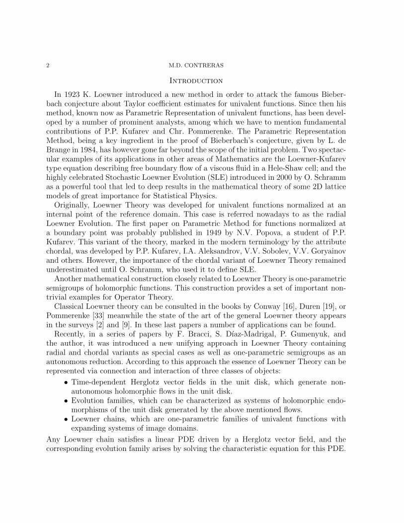
In order to introduce Kufarev’s equation properly, let us fix some notations. Denote byH the upper half-plane. Let γ : [0,+∞)→ H be a Jordan arc with ending point γ(∞) = 0,

24 M.D. CONTRERAS
that is, limt→+∞ γ(t) = 0. Write Ωt := H \ γ[t,+∞). By the Riemann mapping theorem,there exists a conformal transformation f of the unit disk D onto Ωt. By the Caratheodorycontinuity theorem (see Theorem 6.8), the map k has a continuous extension to the closedunit disk. If C is the Cayley transformation from D onto H, which is an automorphism ofthe Riemann sphere, then k := f C−1 : H→ Ωt is a conformal transformation of H ontoΩt. k has a continuos extension to the closure of the upper half-plane. We may assumethat k(∞) =∞. Then there are an interval (α, β) in the real line and a point λ ∈ (α, β)such that
• each segment [α, λ] and [λ, β] is mapped by k homeomorphically onto γ[t,+∞],• ∂H \ [α, β] is mapped homeomorphically onto ∂H \ 0.
Hence, by the Schwarz Reflection Principle, k can be extended to a conformal map k∗ of
C \ [α, β] onto C \ (γ[t,+∞] ∪ γ[t,+∞]). Since k(∞) = ∞, the point ∞ is a pole of k.Conformality of k implies that such pole is simple. Thus
k∗(z) = az + b+∞∑n=1
c∗nz−n
with a 6= 0. Since k∗(z) = k∗(z) for all z ∈ ∂H \ [α, β], we deduce that a, b, and c∗n,
for all n, are real. Moreover, since limy→+∞k(iy)iy
= a and Re k(iy)iy
= Im k(iy)y≥ 0, we have
that a > 0. Consider the automorphism of the upper half-plane given by m(z) = az + b.The map kt := k m−1 is still a conformal transformation from H onto Ωt such thatk(z) = z +
∑∞n=1 cnz
−n for some real coefficients cn. With a similar argument, using thistime that Im (k(z)− z) ≥ 0 for all z ∈ H and that
Re iy(k(iy)− iy) = −yIm (k(iy)− iy)→ c1, as y → +∞,
one can deduce that c1 < 0.Thus kt : H→ H \ γ[t,+∞) can be chosen with the normalization
kt(z) = z − c(t)
z+O
(1
z2
),
with c(t) < 0 for all t. After a reparametrization of the curve γ, one can assume thatc(t) = 2t and there are an interval (αt, βt) in the real line and a point λt ∈ (αt, βt) suchthat
• each segment [αt, λt] and [λt, βt] is mapped by kt homeomorphically onto γ[t,+∞],• ∂H \ [αt, βt] is mapped homeomorphically onto ∂H \ 0.
Under this normalization, one can show that kt satisfies the following partial differentialequation:
(5.1)∂kt(w)
∂t= −k′t(w)
2
w − h(t), (w ∈ H).

LOEWNER’S THEORY 25
: : Im 0w w= >H
0 = γ (∞) = k(αt ) = k(βt )
(0)γ
γ (t) = kt (λt )tk
γ
βtαt 0λt
where h is a continuous real-valued function (see [25]). This equation is known as chordalLoewner PDE.
If we denote by gt = k−1t : Ωt → H, after some elementary calculations, we deduce that
gt(z) = z +2t
z+O
(1
z2
),
and the function t 7→ gt(z) is the solution of the initial value problem
(5.2)∂w
∂t=
−2
w − h(t), with w(0) = z
for all z ∈ H. This equation is known as chordal Loewner ODEFor a complete and detailed proof of these results, the reader can see the book by Lawler
[25] or the paper by del Monaco and Gumenyuk [18].To compare this chordal PDE with the radial Loewner PDE, we should rewrite it in the
unit disk setting. For that, take T : D→ H the biholomorphism T (z) = i z+11−z . Its inverse
is T−1(w) = w−iw+i
. Then ft := T−1 kt T is analytic in the unit disk. Moreover,
∂ft(z)
∂t= (T−1)′(kt(z))
∂kt(T (z))
∂t;
f ′t(z) = (T−1)′(kt(z))k′t(T (z))T ′(z).

26 M.D. CONTRERAS
Thus∂ft(w)
∂t= −f ′t(w)
2
T (z)− h(t)
1
T ′(z)
= −f ′t(w)2
T (z)− h(t)
(1− z)2
2i
= (1− z)2f ′t(w)1
z+11−z + ih(t)
, (z ∈ D).
Notice that the function p(z, t) := 1z+11−z+ih(t)
has non-negative real part and we obtain that
(5.3)∂ft(w)
∂t= (1− z)2f ′t(w)p(z, t), (z ∈ D).
Again, the study of this PDE passes previously through the Initial Value Problem
(5.4)dw
dt= −(1− w)2p(w, t), w(s) = z,
when s ≥ 0 and z ∈ D. In this case, the solution does exist for t ∈ [s, Tz,s). Equations(5.3) and (5.4) are nowadays known as chordal partial or ordinary Loewner differentialequation with the function h as driving term.
6. Prerequisites
6.1. Some results about Riemann mappings and convergence of domains. Inthis section, we provide some results we will use. Most of them are stated without proofs.The reader can see the books by Duren [19] and Pommerenke [33] for their proofs.
Theorem 6.1 (Riemann Mapping Theorem). Let Ω be a simply connected proper domainin C and w0 ∈ Ω. Then there exists a unique biholomorphic function f : D→ Ω such thatf(0) = w0 and f ′(0) > 0.
Exercise 6.2. Find the biholomorphism f from D onto the upper half-plane H such thatf(0) = i and f ′(0) > 0.
Caratheodory gave a complete geometric characterization of the convergence of univa-lent functions in terms of the convergence of their image domains.
Definition 6.3. Let Ωnn∈N be a sequence of simply connected open domains in C, with0 ∈ Ωn for every n ∈ N. We define the kernel of Ωn to be the set Ω as follows:
(1) if 0 is not an interior point of ∩n∈NΩn, then Ω := 0;(2) if 0 is an interior point of ∩n∈NΩn, then Ω is defined as the set of all points w ∈ C
such that there exists a simply connected domain H with 0 ∈ H, w ∈ H such thatH ⊂ Ωn for all sufficiently large n (recall that a domain is open and connected).
We say that the sequence of domains Ωnn∈N converges to Ω if each subsequence Ωnkof Ωn has kernel Ω. In such a case, we write Ωn → Ω.

LOEWNER’S THEORY 27
Example 6.4. If Ωn−1 ⊂ Ωn for any n, then the kernel is Ω = ∪nΩn (this is the uniquecase we will need in these notes).
Example 6.5. Let Γ be a Jordan curve, take Ω the unique bounded connected componentof C\Γ. Assume that 0 ∈ Ω. Given w0 ∈ Γ, consider a Jordan arc Γ starting at w0, endingat ∞ and which does not intersect Ω \ w0. Let wn ⊂ Γ such that wn moves clockwiseon Γ and such that wn → w0. Consider
γn := Γ ∪ “ the portion of Γ from w0 to wn” (see the picture)
and Ωn = C \ γn. Then Ωn → Ω.
Theorem 6.6 (Caratheodory kernel theorem, also known as Caratheodory convergencetheorem). Let Ωnn∈N be a sequence of open domains in C, with 0 ∈ Ωn for every n ∈ N.Let fn : D → C be univalent, fn(0) = 0, f ′n(0) > 0, and such that Ωn = fn(D). Then(fn) converges uniformly on compacta of D to a univalent function f if and only if Ωnconverges to a domain Ω and Ω 6= C. Furthermore, f(D) = Ω and f−1
n converges to f−1
uniformly on each compact subset of Ω.
Proof. Suppose that (fn) converges uniformly on compacta of D to the univalent functionf and write Ω := f(D). Write ∆ the kernel of the sequence Ωn . We must prove thatΩ = ∆. Once we have proved this fact, since any subsequence of (fn) also converges to fit follows that the kernel of any subsequence of Ωn has the same kernel so that Ωnconverges to Ω.
Since the limit function is univalent, we have that Ω 6= C.Take w0 = f(z0) ∈ Ω, w0 6= 0. Choose r such that |z0| < r < 1. Then the domain
H = f(z) : |z| ≤ r contains 0 and w0. We will prove that H ⊂ Ωn for all n largeenough. Suppose this is false. Then there is a subsequence (nk) and points wk ∈ H suchthat wk /∈ Ωnk . Since we may take another subsequence if necessary we may assume thatwk → w∗ for some w∗ ∈ H. Since fnk(z)−wk 6= 0 for z ∈ D and fnk −wk converges oncompacta to the non-constant function f−w∗, we therefore obtain from Hurwitz’ theoremthat f(z)− w∗ 6= 0 for z ∈ D. This contradicts w∗ ∈ H ⊂ f(D). Thus H, and then f(D),is contains in the kernel ∆.

28 M.D. CONTRERAS
Take w0 6= 0 a point of ∆. There is a domain H containing 0 and w0 and such thatH ⊂ Ωn for n bigger than a certain n0. The inverse function f−1
n is analytic in H and|f−1n (z)| < 1. By Montel’s theorem there is a subsequence f−1
nkthat converges uniformly
on compact subsets in H. The limit function g satisfies that g(0) = 0 and |g(w)| ≤ 1 forall w ∈ H. Thus, |g(w)| < 1 for all w. It follows that fnk converges locally uniformly nearthe point g(w0). Thus w0 = fnk(f
−1nk
(w0)) and w0 = f(g(w0)) ∈ f(D). Notice that thisimplies that g is nothing but f−1 on H.
We have proved that ∆ = f(D) but also above arguments show that f−1n converges to
f−1 uniformly on each compact subset of Ω.Conversely, assume that Ωn converges to its kernel Ω 6= C. First we show that the
sequence (fn) is a normal family. By Koebe one-quarter theorem,
w : |w| < 1
4f ′n(0) ⊆ Ωn.
If the sequence (f ′n(0)) is not bounded, then the kernel of Ωn is C, getting a contradiction.By Koebe distortion theorem (see the inequalities (1.6) in Theorem 1.8), we have that
|fn(z)| ≤ |f ′n(0)| |z|(1− |z|)2
(z ∈ D).
Since the sequence (f ′n(0)) is bounded, we see that (fn) is locally uniformly bounded andtherefore normal.
Take any convergent subsequence (fnk) with limit f uniformly. Since f(0) = 0, we havethat either f is univalent or f is identically zero. Assume that f ≡ 0. Since Ωn convergesto a domain Ω and 0 ∈ Ω, there is ρ > 0 such that D(0, ρ) ⊂ Ωn for all n. The inversefunctions f−1
n is defined in D(0, ρ), f−1n (0) = 0, and |f−1
n (w)| ≤ 1, for all |w| ≤ ρ. Schwarzlemma implies that |(f−1
n )′(0)| ≤ 1/ρ. Thus |f ′n(0)| ≥ ρ for all n, which contradicts theassumption that (fnk) converges uniformly to zero on compacta. Thus f is univalent.
We claim that (fn) converges locally uniformly in D. Suppose this is false. In such acase, using the normality, we can find two subsequences (fnk) and (fmk) that convergelocally uniformly to two different univalent functions f and g. In view of what we havealready proved the sequences of domains Ωnk and Ωmk converges to f(D) and g(D).By hypothesis, f(D) = g(D). Since f(0) = g(0) = 0 and f ′(0) > 0 and g′(0) > 0, itfollows from the uniqueness part of the Riemann mapping theorem that f = g, whereasthese functions were supposed to be different. Thus we have proved that the sequence(fn) converge to a univalent function f uniformly on compacta.
Using Example 6.5 and Caratheodory kernel theorem one obtain that the Riemann mapof the inner domain of Jordan curve can be approximated by the Riemann map of a familyof slit domains. Bearing in mind this remark, the reader should do the next exercise.
Exercise 6.7. Consider the subclass
S ′ = f ∈ S : f(D) is the whole plane C slit along a Jordan arc Γ.
LOEWNER’S THEORY 29
Prove that S ′ is dense in S when we endowed S with the topology of the uniform convergeon compacta.
With this exercise, it is possible to reduce the study of some extremal problems in Sto the subclass S ′.
Next result is due to Caratheodory and it can be seen in [34, page 18].
Theorem 6.8 (Continuity theorem). Let f be a Riemann map of a domain Ω. Then fhas a continuous extension to D if and only if ∂Ω is locally connected.
Theorem 6.9. Let f be a conformal map. Then the pre-image under f of a slit of f(D)is a slit of D.
See [38, page 162] for a proof of above theorem.
6.2. Distortion results for functions with non-negative real parts. In this subsec-tion we deal with some elementary properties of analytic functions with non-negative realparts. They are based on the Herglotz representation Theorem for harmonic functions.
Next selection theorem can be seen in [19, page 22].
Theorem 6.10 (Helly Selection Theorem). Let αn be a sequence of nondecreasing func-tions on a bounded interval [a, b], with αn(a) = 0 and αn(b) = 1. Then some subsequenceαnk converges everywhere in [a, b] to a nondecreasing function α, and for each functionf continuous on [a, b],
limk→∞
∫ b
a
f(t) dαnk(t) =
∫ b
a
f(t) dα(t).
Theorem 6.11 (Herglotz representation Theorem). Let u be a positive harmonic functionin D with u(0) = 1. Then there exists a unique increasing function µ : [0, 2π] → R suchthat µ(2π)− µ(0) = 1 and
u(reiθ) =
∫ 2π
0
P (r, θ − t)dµ(t), r < 1,
where, as usual, P is the Poisson kernel of D given by
P (r, θ) =1− r2
1− 2r cos θ + r2= Re
1 + reiθ
1− reiθ
, r < 1.
Proof. For r < 1, define
µr(t) =1
2π
∫ t
0
u(reiθ) dθ, r < 1.
Then µr is an increasing function with µr(0) = 0 and µr(2π) = u(0) = 1. By the Helleyselection theorem, there is a sequence rn increasing to 1 for which µrn(t) → µ(t), a
30 M.D. CONTRERAS
nondecreasing function on [0, 2π]. By the Poisson formula,
u(rnz) =1
2π
∫ 2π
0
P (r, θ − t)u(rneit) d(t) =
∫ 2π
0
P (r, θ − t) durn(t),
where z = reiθ ∈ D. Letting n → ∞ and appealing to the integration part of the Hellyselection theorem, we obtain the desired representation.
We leave for the reader the uniqueness of µ (see for example the book by Duren [19,page 24]).
Corollary 6.12. Let p : D→ C be analytic with Re p(z) ≥ 0 for all z. Then there existsan increasing function µ : [0, 2π]→ R such that µ(2π)− µ(0) = Re p(0) and
(6.1) p(z) =
∫ 2π
0
eit + z
eit − zdµ(t) + iIm p(0).
Proof. Consider the harmonic function u = Re p. By above theorem, there is an increasingfunction µ : [0, 2π]→ R such that µ(2π)− µ(0) = Re p(0) and
u(reiθ) =
∫ 2π
0
Re
1 + rei(θ−t)
1− rei(θ−t)
dµ(t) =
∫ 2π
0
Re
eit + reiθ
eit − reiθ
dµ(t)
= Re
∫ 2π
0
eit + reiθ
eit − reiθdµ(t), r < 1.
That is, the analytic functions p and z 7→∫ 2π
0eit+zeit−zdµ(t) have the same real part. Thus,
p(z)−∫ 2π
0eit+zeit−zdµ(t) is constant. But p(0)−
∫ 2π
0eit+0eit−0
dµ(t) = p(0)−Re p(0) = iIm p(0).
Proposition 6.13. Let p(z) = 1 + c1z+ c2z2 + c3z
3 + ... be analytic in D with Re p(z) ≥ 0for all z ∈ D. Then
(1) (Re c1)2 ≤ 2 + Re c2;(2) |cn| ≤ 2 for all n.
(3) |p(z)| ≤ 1+|z|1−|z| for all z ∈ D.
(4) |p′(z)| ≤ 2(1−|z|)2 for all z ∈ D.
Proof. (1) The function ψ(z) := 1z
1−p(z)1+p(z)
is an analytic self-map of the unit disk. By
Schwarz Lemma we have that |ψ′(0)| ≤ 1− |ψ(0)|2. That is∣∣∣∣12c2 −1
4c2
1
∣∣∣∣ ≤ 1− 1
4|c1|2.
Taking the negative real part on the left-hand side we conclude that
2 + Re c2 ≥1
2Re c2
1 +1
2|c1|2 = (Re c1)2.

LOEWNER’S THEORY 31
(2) Take µ as in (6.1). Since p(0) = 1, we have that
p(z) =
∫ 2π
0
eit + z
eit − zdµ(t).
From the equality
eit + z
eit − z= 1 + 2
∞∑n=1
e−itnzn,
we deduce that cn = 2∫ 2π
0e−itndµ(t), so that
|cn| ≤ 2
∫ 2π
0
|e−itn|dµ(t) = 2(µ(2π)− µ(0)) = 2.
(3) Using the notation introduced in the proof of statement (2) we have that
|p(z)| ≤∫ 2π
0
∣∣∣∣eit + z
eit − z
∣∣∣∣ dµ(t) ≤∫ 2π
0
1 + |z|1− |z|
dµ(t) =1 + |z|1− |z|
.
(4) Since p′(z) =∫ 2π
02eit
(eit−z)2dµ(t), we have that
|p′(z)| ≤∫ 2π
0
2
|eit − z|2dµ(t) ≤
∫ 2π
0
2
(1− |z|)2dµ(t) =
2
(1− |z|)2.
Notice that one can have equality in the four statements of above lemma. Namely, takethe function p(z) = 1+z
1−z = 1 + 2∑∞
n=1 zn.
6.3. Convergence of analytic functions.
Theorem 6.14 (Vitali’s Theorem). Let Ω be a domain in the complex plane and fna sequence in Hol(Ω). Assume that for every compact set K of Ω there exists a constantM > 0 such that |fn(z)| ≤ M for all z ∈ K and all n. Assume that the set A := z ∈Ω : limn fn(z) exists has an accumulation point in Ω. Then there is f ∈ Hol(Ω) such thatlimn fn = f uniformly on compact subsets of Ω.
Theorem 6.15 (Hurwitz’s Theorem). Let Ω be a region and suppose that the sequencefn in Hol(Ω) converges to f .
• If D(a,R) ⊂ Ω and f(z) 6= 0 for z ∈ ∂D(a,R) then there is an integer N such thatfor all n ≥ N , the functions f and fn have the same number of zeros in D(a,R).• Either f(z) ≡ 0 in D, or every zero of f is a limit-point of a sequence of zeros ofthe functions fn.
Remark 6.16. Notice that if fn converges to f uniformly in compact sets of D, f isunivalent and r < 1, then there is n0 such that fn is univalent in rD, for all n ≥ n0.
As a consequence of Hurwitz’s Theorem one can prove:

32 M.D. CONTRERAS
Theorem 6.17. If (fn) is a sequence of univalent functions in Ω and converges uniformlyon compacta to f , then f is either univalent or constant.
References
[1] M. Abate, Iteration Theory of Holomorphic Maps on Taut Manifolds, Mediterranean Press, Rende,Cosenza, 1989.
[2] M. Abate, F. Bracci, M.D. Contreras, and S. Dıaz-Madrigal, The evolution of Loewner’s differen-tial equation, Newsletter of the European Mathematical Society, 78, (2010), 31-38. Available onhttp://personal.us.es/contreras/1-ems-abate-etal.pdf
[3] L. Arosio, F. Bracci, H. Hamada, G. Kohr, Loewner’s theory on complex manifolds, to appear inJ. Anal. Math. Available on ArXiv:1002.4262.
[4] J. Becker, Lownersche Differentialgleichung und quasikonform fortsetzbare schlichte Funktionen, J.Reine Angew. Math. 255 (1972) 23–43.
[5] E. Berkson and H. Porta, Semigroups of analytic functions and composition operators, MichiganMath. J. 25 (1978) 101–115.
[6] F. Bracci, M.D. Contreras, S. Dıaz-Madrigal, Pluripotential theory, semigroups and boundary be-havior of infinitesimal generators in strongly convex domains, J. Eur. Math. Soc. 12 (2010) 23–53.
[7] F. Bracci, M.D. Contreras, and S. Dıaz-Madrigal, Evolution Families and the Loewner Equation I:the unit disk, Journal fur die reine und angewandte Mathematik (Crelle’s Journal), 672 (2012), 1–37.
[8] F. Bracci, M.D. Contreras, and S. Dıaz-Madrigal, Evolution Families and the Loewner Equation II:complex hyperbolic manifolds. Math. Ann., 344 (2009), 947–962.
[9] F. Bracci, M.D. Contreras, S. Dıaz-Madrigal, and A. Vasiliev, Classical and stochastic Lowner-Kufarev equations. Preprint.
[10] L. Carleson, N. Makarov, Aggregation in the plane and Loewner’s equation, Comm. Math. Phys. 216(2001) 583–607.
[11] M. D. Contreras and S. Dıaz-Madrigal, Analytic flows in the unit disk: angular derivatives and bound-ary fixed points, Pacific Journal of Mathematics, 222 (2005), 253-286.
[12] M.D. Contreras, S. Dıaz-Madrigal, P. Gumenyuk, Loewner chains in the unit disc, Rev. Mat.Iberoamericana 26 (2010) 975–1012.
[13] M.D. Contreras, S. Dıaz-Madrigal, P. Gumenyuk, Local duality in Loewner equations, Preprint.[14] M. D. Contreras, S. Dıaz-Madrigal, and Ch. Pommerenke, Fixed points and boundary behaviour of
the Koenigs function, Annales Academiae Scientiarum Fennicae, Mathematica, 29 (2004), 471-488.[15] M. D. Contreras, S. Dıaz-Madrigal, and Ch. Pommerenke, On boundary critical points for semigroups
of analytic functions, Mathematica Scandinavica, 98 (2006), 125-142.[16] J.B. Conway, Functions of one complex variable, II. Second edition. Graduate Texts in Mathematics,
159. Springer-Verlag, New York-Berlin, 1996.[17] L. de Branges, A proof of the Bieberbach conjecture, Acta Math. 154 (1985) 137–152.[18] A. del Monaco and P. Gumenyuk, Chordal Loewner Equation, Preprint.[19] P.L. Duren, Univalent Functions, Springer, New York, 1983.[20] C.H. FitzGerald, Ch. Pommerenke, The de Branges theorem on univalent functions, Trans. Amer.
Math. Soc. 290 (1985) 683–690.[21] B. Gustafsson, A. Vasil’ev, Conformal and potential analysis in Hele-Shaw cells, Birkhauser, 2006.[22] T.E. Harris, The Theory of Branching Processes. Corrected reprint of the 1963 original, Dover
Phoenix Editions, Dover Publications, Inc., Mineola, NY, 2002.[23] P.P. Kufarev, On one-parameter families of analytic functions (in Russian. English summary),
Rec. Math. [Mat. Sbornik] N.S. 13 (55) (1943), 87–118.
LOEWNER’S THEORY 33
[24] G.F. Lawler, An introduction to the stochastic Loewner evolution, in Random Walks and Geometry,V. Kaimonovich, ed., de Gruyter (2004), 261–293.
[25] G.F. Lawler, Conformally Invariant Processes in the Plane, Mathematical Surveys and Monographs,Vol. 114, AMS, 2005.
[26] G.F. Lawler, O. Schramm, W. Werner, Values of Brownian intersection exponents. I. Half-planeexponents, Acta Math. 187 (2001) 237–273.
[27] G.F. Lawler, O. Schramm, W. Werner, Values of Brownian intersection exponents. II. Plane expo-nents, Acta Math. 187 (2001) 275–308.
[28] J.R. Lind, A sharp condition for the Loewner equation to generate slits, Ann. Acad. Sci. Fenn. Math.30 (2005) 143–158.
[29] J.R. Lind, D.E. Marshall, S. Rohde, Collisions and spirals of Loewner Traces, to appear in DukeMath. J., 154 (2010), 527–573.
[30] K. Lowner, Untersuchungen uber schlichte konforme Abbildungen des Einheitskreises. I, Math. Ann.89 (1923) 103–121.
[31] D.E. Marshall, S. Rohde, The Loewner differential equation and slit mappings, J. Amer. Math. Soc.18 (2005) 763–778.
[32] Ch. Pommerenke, Uber dis subordination analytischer funktionen, J. Reine Angew Math. 218 (1965),159–173.
[33] Ch. Pommerenke, Univalent Functions. With a chapter on quadratic differentials by Gerd Jensen,Vandenhoeck & Ruprecht, Gottingen, 1975.
[34] Ch. Pommerenke, Boundary Behaviour of Conformal Maps, Springer-Verlag, Berlin, 1992.[35] S. Reich, D. Shoikhet, Nonlinear Semigroups, Fixed Points, and Geometry of Domains in Banach
Spaces, Imperial College Press, London, 2005.[36] M. Rosenblum and J. Rovnyak, Topics in Hardy classes and univalent functions, Birkhauser, 1994.[37] O. Schramm, Scaling limits of loop-erased random walks and uniform spanning trees, Israel J. Math.
118 (2000) 221–288.[38] J. H. Shapiro, Composition Operators and Classical Function Theory, Springer-Verlag, New York,
1993.[39] A.G. Siskakis, Semigroups of composition operators and the Cesaro operator on Hp(D), Ph. D.
Thesis, University of Illinois, 1985.[40] A.G. Siskakis, Semigroups of composition operators on spaces of analytic functions, a review, Con-
temp. Math. 213 (1998) 229–252.[41] A. Vasil’ev, From Hele-Shaw experiment to integrable systems: a historical overview. Compl. Anal.
Oper. Theory 3 (2009) 551-585.
Camino de los Descubrimientos, s/n, Departamento de Matematica Aplicada II, EscuelaTecnica Superior de Ingenierıa, Universidad de Sevilla, 41092, Sevilla, Spain.
E-mail address: [email protected]