LOG-D N : HOW TO SPARSIFY A DENSENET - arXiv

Published as a conference paper at ICLR 2018

LOG-DENSENET: HOW TO SPARSIFY A DENSENET

Hanzhang Hu1, Debadeepta Dey2, Allison Del Giorno1, Martial Hebert1 & J. Andrew Bagnell11 Carnegie Mellon UniversityPittsburgh, PA, USA{hanzhang,adelgior,hebert,dbagnell}@cs.cmu.edu

2 Microsoft ResearchRedmond, WA, [email protected]

ABSTRACT

Skip connections are increasingly utilized by deep neural networks to improveaccuracy and cost-efficiency. In particular, the recent DenseNet is efficient incomputation and parameters, and achieves state-of-the-art predictions by directlyconnecting each feature layer to all previous ones. However, DenseNet’s extremeconnectivity pattern may hinder its scalability to high depths, and in applicationslike fully convolutional networks, full DenseNet connections are prohibitively ex-pensive. This work first experimentally shows that one key advantage of skip con-nections is to have short distances among feature layers during backpropagation.Specifically, using a fixed number of skip connections, the connection patternswith shorter backpropagation distance among layers have more accurate predic-tions. Following this insight, we propose a connection template, Log-DenseNet,which, in comparison to DenseNet, only slightly increases the backpropagationdistances among layers from 1 to (1 + log2 L), but uses only L log2 L total con-nections instead of O(L2). Hence, Log-DenseNets are easier than DenseNets toimplement and to scale. We demonstrate the effectiveness of our design principleby showing better performance than DenseNets on tabula rasa semantic segmen-tation, and competitive results on visual recognition.

1 INTRODUCTION

Deep neural networks have been improving performance for many machine learning tasks, scalingfrom networks like AlexNet (Krizhevsky et al., 2012) to increasingly more complex and expensivenetworks, like VGG (Simonyan & Zisserman, 2014), ResNet (He et al., 2016) and Inception (Chris-tian Szegedy & Alemi, 2017). Continued hardware and software advances will enable us to builddeeper neural networks, which have higher representation power than shallower ones. However,the payoff from increasing the depth of the networks only holds in practice if the networks can betrained effectively. It has been shown that naıvely scaling up the depth of networks actually de-creases the performance (He et al., 2016), partially because of vanishing/exploding gradients in verydeep networks. Furthermore, in certain tasks such as semantic segmentation, it is common to takea pre-trained network and fine-tune, because training from scratch is difficult in terms of both com-putational cost and reaching good solutions. Overcoming the vanishing gradient problem and beingable to train from scratch are two active areas of research.

Recent works attempt to overcome these training difficulties in deeper networks by introducingskip, or shortcut, connections (Long et al., 2015; Hariharan et al., 2015; Srivastava et al., 2015;He et al., 2016; Larsson et al., 2017; Huang et al., 2017) so the gradient reaches earlier layers andcompositions of features at varying depth can be combined for better performance. In particular,DenseNet (Huang et al., 2017) is the extreme example of this, concatenating all previous layers toform the input of each layer, i.e., connecting each layer to all previous ones. However, this incurs anO(L2) run-time complexity for a depth L network, and may hinder the scaling of networks. Specif-ically, in fully convolutional networks (FCNs), where the final feature maps have high resolution sothat full DenseNet connections are prohibitively expensive, Jegou et al. (2017) propose to cut mostof connections from the mid-depth. To combat the scaling issue, Huang et al. (2017) propose tohalve the total channel size a number of times. Futhermore, Liu et al. (2017) cut 40% of the chan-nels in DenseNets while maintaining the accuracy, suggesting that much of the O(L2) computationis redundant. Therefore, it is both necessary and natural to consider a more efficient design principlefor placing shortcut connections in deep neural networks.

1

arX

iv:1

711.

0000

2v1

[cs

.CV

] 3

0 O

ct 2

017


In this work, we address the scaling issue of skip connections by answering the question: if we canonly afford the computation of a limited number of skip connections and we believe the networkneeds to have at least a certain depth, where should the skip connections be placed? We designexperiments to show that with the same number of skip connections at each layer, the networks canhave drastically different performance based on where the skip connections are. In particular, wesummarize this result as the following design principle, which we formalize in Sec. 3.2: given afixed number of shortcut connections to each feature layer, we should choose these shortcutconnections to minimize the distance among layers during backpropagation.

Following this principle, we design a network template, Log-DenseNet. In comparison to DenseNetsat depth L, Log-DenseNets cost only L logL, instead of O(L2) run-time complexity. Furthermore,Log-DenseNets only slightly increase the short distances among layers during backpropagation from1 to 1+logL. Hence, Log-DenseNets can scale to deeper and wider networks, even without customGPU memory managements that DenseNets require. In particular, we show that Log-DenseNetsoutperform DenseNets on tabula rasa semantic segmentation on CamVid (Brostow et al., 2008),while using only half of the parameters, and similar computation. Log-DenseNets also achievecomparable performance to DenseNet with the same computations on visual recognition data-sets,including ILSVRC2012 (Russakovsky et al., 2015). In short, our contributions are as follows:

• We experimentally support the design principle that with a fixed number of skip connections perlayer, we should place them to minimize the distance among layers during backpropagation.• The proposed Log-DenseNets achieve small 1 + log2 L between-layer distances using few con-

nections (L log2 L), and hence, are scalable for deep networks and applications like FCNs.• The proposed network outperforms DenseNet on CamVid for tabula rasa semantic segmentation,

and achieves comparable performance on ILSVRC2012 for recognition.

2 BACKGROUND AND RELATED WORKS

Skip connections. The most popular approach to creating shortcuts is to directly add features fromdifferent layers together, with or without weights. Residual and Highway Networks (He et al.,2016; Srivastava et al., 2015) propose to sum the new feature map at each depth with the onesfrom skip connections, so that new features can be understood as fitting residual features of theearlier ones. FractalNet (Larsson et al., 2017) explicitly constructs shortcut networks recursivelyand averages the outputs from the shortcuts. Such structures prevent deep networks from degradingfrom the shallow shortcuts via “teacher-student” effects. (Huang et al., 2016) implicitly constructsskip connections by allowing entire layers to be dropout during training. DualPathNet (Chen et al.,2017) combines the insights of DenseNet (Huang et al., 2017) and ResNet (He et al., 2016), andutilizes both concatenation and summation of previous features.

Run-time Complexity and Memory of DenseNets. DenseNet (Huang et al., 2017) emphasizesthe importance of compositional skip connections and it is computationally efficient (in accuracyper FLOP) compared to many of its predecessors. One intuitive argument for the cost-efficiency ofDenseNet is that the layers within DenseNet are directly connected to each other, so that all layerscan pick up training signals easily, and adjust accordingly. However, the quadratic complexity mayprevent DenseNet from scale to deep and wide models. In fact at each downsampling, DenseNetapplies block compression, which halves the number of channels in the concatenation of previouslayers. DenseNet also opts not to double the output channel size of conv layers after downsam-pling, which divides the computational cost of each skip connection. These design choices enableDenseNets to be deep for image classification where final layers have low resolutions. However,final layers in FCNs for semantic segmentation have higher resolution than in classification. Hence,to fit models in the limited GPU memory, FC-DenseNets (Jegou et al., 2017) have to cut most oftheir skip connections from mid-depth layers. Furthermore, a naıve implementation of DenseNetrequires O(L2) memory, because the inputs of the L convolutions are individually stored, and theycost O(L2) memory in total. Though there exist O(L) implementations via memory sharing amonglayers (Liu, 2017), they require custom GPU memory management, which is not supported in manyexisting packages. Hence, one may have to use custom implementations and recompile packageslike Tensorflow and CNTK for memory efficient Densenets, e.g., it costs a thousand lines of C++ onCaffe (Li, 2016). Our work recognizes the contributions of DenseNet’s architecture to utilize skipconnections, and advocates for the efficient use of compositional skip connections to shorten thedistances among feature layers during backpropagation. Our design principle can especially help

2


applications like FC-DenseNet (Jegou et al., 2017) where the network is desired to be at least acertain depth, but only a limited number of shortcut connections can be formed.

Network Compression. A wide array of works have proposed methods to compress networks byreducing redundancy and computational costs. (Denton et al., 2014; Kim et al., 2016; Ioannou et al.,2016) decompose the computation of convolutions at spatial and channel levels to reduce convolu-tion complexity. (Hinton et al., 2014; Ba & Caruana, 2014) propose to train networks with smallercosts to mimic expensive ones. (Liu et al., 2017) uses L1 regularization to cut 40% of channels inDenseNet without losing accuracy. These methods, however, cannot help in applications that cannotfit the complex networks in GPUs in the first place. This work, instead of cutting connections arbi-trarily or post-design, advocates a network design principle to place skip connections intelligentlyto minimize between-layer distances.

3 FROM DENSENET TO LOG-DENSENET

3.1 PRELIMINARY ON DENSENETS

Formally, we call the feature layers in a feed-forward convolutional network as x0, x1, ..., xL, wherex0 is the feature map from the initial convolution on the input image x, and each of the subsequentxi is from a transformation fi with parameter θi that takes input from a subset of x0, ..., xi−1. Inparticular, the traditional feed-forward networks have xi = fi(xi−1; θi), and the skip connectionsallow fi to utilize more than just xi−1 for computing xi. Following the trend of utilizing skip con-nections to previous layers (He et al., 2016; Srivastava et al., 2015; Larsson et al., 2017), DenseNet(Huang et al., 2017) proposes to form each feature layer xi using all previous features layers, i.e.,

xi = fi(concat({xj : j = 0, ..., i− 1}) ; θi), (1)

where concat(•) concatenates all features in its input collection along the feature channel dimen-sion. Each fi is a bottleneck structure (Huang et al., 2017), BN-ReLU-1x1conv-BN-ReLU-3x3conv,where the final conv produces g, the growth rate, number of channels, and the bottleneck 1x1 convproduces 4g channels of features out of the merged input features. DenseNet also organizes lay-ers into nblock number of blocks. Between two contiguous blocks, there is a 1x1conv-BN-ReLU,followed by an average pooling, to transform and downsample all previous features maps togetherto a coarser resolution. In practice, nblock ≤ 4 in almost all state-of-the-art visual recognition ar-chitectures (He et al., 2016; Christian Szegedy & Alemi, 2017; Huang et al., 2017). The directconnections among layers in DenseNet are argued to be the key reason why DenseNets enjoy highefficiency in parameter and computation to achieve the state-of-the-art predictions: the direct con-nections introduce implicit deep supervision (Lee et al., 2015) in intermediate layers, and reduce thevanishing/exploding gradient problem by enabling direct influence between any two feature layers.

3.2 MAXIMUM BACKPROPAGATION DISTANCE

We now formally define the proposed design principle that with the same number of connections,the distance between any two layers during backpropagation should be as small as possible. Weconsider each xi as a node in a graph, and the directed edge (xi, xj) exists if xi takes direct inputfrom xj . The backpropagation distance (BD) from xi to xj (i > j) is then the length of the shortestpath from xi to xj on the graph. Then we define the maximum backpropagation distance (MBD) asthe maximum BD among all pairs i > j. Then DenseNet has a MBD of 1, if we disregard transitionlayers. To reduce the O(L2) computation and memory footprint of DenseNet, we propose Log-DenseNet which increase MBD slightly to 1 + log2 L while using only O(L logL) connections andrun-time complexity. Since the current practical networks have less than 2000 depths, the proposedmethod has a MBD of at most 7 to 11.

3.3 LOG-DENSENET

For simplicity, we let log(•) denote log2(•). In a proposed Log-Dense Network, each layer i takesdirect input from at most log(i) + 1 number of previous layers, and these input layers are exponen-tially apart from depth i with base 2, i.e.,

xi = fi(concat({xi−b2ke : k = 0, ..., blog(i)c}) ; θi), (2)

where b•e is the nearest integer function and b•c is the floor function. For example, the inputfeatures for layer i are layer i − 1, i − 2, i − 4, .... We define the input index set at layer i to

3


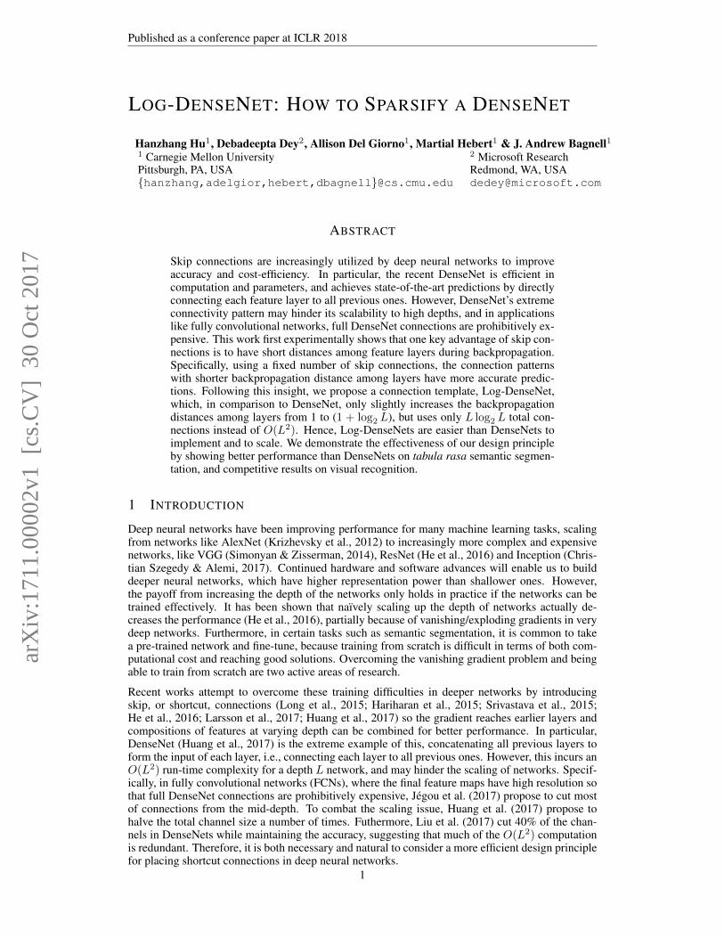
(a) DenseNet (b) Log-DenseNet V1 (c) Log-DenseNet V2 (d) LogLog-DenseNet

Figure 1: Connection illustration for L = 24. Layer 0 is the initial convolution. (i, j) is black meansxj takes input from xi; it is white if otherwise. We assume there is a block transition at depth 12 forLog-DenseNet V2. LogLog-DenseNet is a connection strategy that has 2+log logL MBD.

be {i− b2ke : k = 0, ..., blog(i)c}. We illustrate the connection in Fig. 1b. Since the complexity oflayer i is log(i)+1, the overall complexity of a Log-DenseNet is

∑Li=1(log(i)+1) ≤ L+L logL =

Θ(L logL), which is significantly smaller than the quadratic complexity, Θ(L2), of a DenseNet.

Log-DenseNet V1: independent transition. Following Huang et al. (2017), we organize layersinto blocks. Layers in the same block have the same resolution; the feature map side is halved aftereach block. In between two consecutive blocks, a transition layer will shrink all previous layers sothat future layers can use them in Eq 2. We define a pooling transition as a 1x1 conv followed by a2x2 average pooling, where the output channel size of the conv is the same as the input one. We referto xi after t number of pooling transition as x(t)i . In particular, x(0)i = xi. Then at each transitionlayer, for each xi, we find the latest x(t)i , i.e., t = max{s ≥ 0 : x

(s)i exists}, and compute x(t+1)

i .We abuse the notation xi when it is used as an input of a feature layer to mean the appropriatex(t)i so that the output and input resolutions match. Unlike DenseNet, we independently process

each early layer instead of using a pooling transition on the concatenated early features, becausethe latter option results in O(L2) complexity per transition layer, if at least O(L) layers are to beprocessed. Since Log-DenseNet costsO(L) computation for each transition, the total transition costis O(L logL) as long as we have O(logL) transitions.

Log-DenseNet V2: block compression. Unfortunately, many neural network packages, such asTensorFlow, cannot compute the O(L) 1x1 conv for transition efficiently: in practice, this O(L)operation costs about the same wall-clock time as the O(L2)-cost 1x1 conv on the concatenation oftheO(L) layers. To speed up transition and to further reduce MBD, we propose a block compressionfor Log-DenseNet similar to the block compression in DenseNet (Huang et al., 2017). At eachtransition, the newly finished block of feature layers are concatenated and compressed into g logLchannels using 1x1 conv. The other previous compressed features are concatenated, followed by a1x1 conv that keep the number of channels unchanged. These two blocks of compressed featuresthen go through 2x2 average pooling to downsample, and are then concatenated together. Fig. 1cillustrates how the compressed features are used when nblock = 3, where x0, the initial conv layerof channel size 2g, is considered the initial compressed block. The total connections and run-timecomplexity are stillO(L logL), at any depth the total channel from the compressed feature is at most(nblock − 1)g logL + 2g, and we assume nblock ≤ 4 is a constant. Furthermore, these transitionscost O(L logL) connections and computation in total, since compressing of the latest block costsO(L logL) and transforming the older blocks costs O(log2 L).

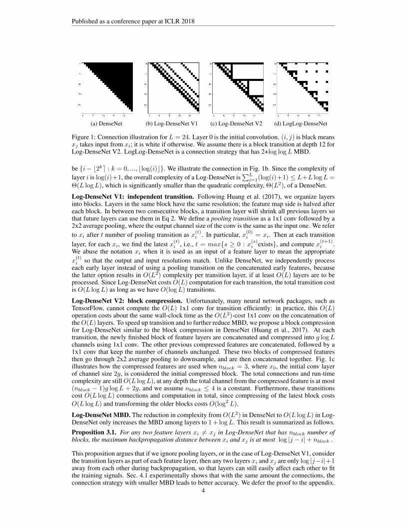
Log-DenseNet MBD. The reduction in complexity from O(L2) in DenseNet to O(L logL) in Log-DenseNet only increases the MBD among layers to 1 + logL. This result is summarized as follows.

Proposition 3.1. For any two feature layers xi 6= xj in Log-DenseNet that has nblock number ofblocks, the maximum backpropagation distance between xi and xj is at most log |j − i|+ nblock .

This proposition argues that if we ignore pooling layers, or in the case of Log-DenseNet V1, considerthe transition layers as part of each feature layer, then any two layers xi and xj are only log |j−i|+1away from each other during backpropagation, so that layers can still easily affect each other to fitthe training signals. Sec. 4.1 experimentally shows that with the same amount the connections, theconnection strategy with smaller MBD leads to better accuracy. We defer the proof to the appendix.

4


CIFAR10 CIFAR100 SVHN(n,g) L N E L N E L N E

(12,16) 7.23 7.59 7.45 29.14 30.59 30.72 2.03 2.11 2.27(12,24) 5.98 6.46 6.56 26.36 26.96 27.80 1.94 2.10 2.05(12,32) 5.48 6.00 6.15 24.21 24.70 25.57 1.85 1.92 1.90(32,16) 5.96 6.45 6.21 25.32 27.48 26.81 1.97 1.94 1.96(32,24) 5.03 5.74 5.43 22.73 25.08 24.80 1.77 1.82 1.95(32,32) 4.81 5.65 4.94 21.77 23.79 23.87 1.76 1.82 1.95(52,16) 5.13 6.80 6.09 23.45 27.99 26.58 1.66 1.98 1.85(52,24) 4.34 5.83 5.03 20.99 26.07 24.19 1.64 1.90 1.80(52,32) 4.56 6.10 4.98 20.58 24.79 23.10 1.72 1.89 1.78

Table 1: Error rates of Log-DenseNet V1(L), NEAREST (N) and EVENLY-SPACED (E), in eachof which layer xi has log i previous layers as input. (L) has a MBD of 1 + logL, and the other twohave L

logL . (L) outperforms the other two clearly. These networks do not have bottlenecks.

In comparison to Log-DenseNet V1, V2 reduces the BD between any two layers from differentblocks to be at most nblock, where the shortest paths go through the compressed blocks.

It is also possible to provably achieve 2+log logLMBD using only 1.5L log logL+o(L log logL)shortcut connections (Fig. 1d), but we defer this design to the appendix, because it has a complexconstruction and involves other factors that affect the prediction accuracy.

Deep supervision. Since we cut the majority of the connections in DenseNet when forming Log-DenseNet, we found that having additional training signals at the intermediate layers using deepsupervision (Lee et al., 2015) for the early layers helps the convergence of the network, even thoughthe original DenseNet does not see performance impact from deep supervision. For simplicity, weplace the auxiliary predictions at the end of each block. Let xi be a feature layer at the end of ablock. Then the auxiliary prediction at xi takes as input xi along with xi’s input features. Following(Hu et al., 2017), we put half of the total weighting in the final prediction and spread the other halfevenly. After convergence, we take one extra epoch of training optimizing only the final prediction.We found this results in the lower validation error rate than always optimizing the final loss alone.

4 EXPERIMENTS

For visual recognition, we experiment on CIFAR10, CIFAR100 (Krizhevsky & Hinton, 2009),SVHN (Netzer et al., 2011), and ILSVRC2012 (Russakovsky et al., 2015).1 We follow (He et al.,2016; Huang et al., 2017) for the training procedure and parameter choices. Specifically, we opti-mize using stochastic gradient descent with a moment of 0.9 and a batch size of 64 on CIFAR andSVHN. The learning rate starts at 0.1 and is divided by 10 after 1/2 and 3/4 of the total iterations aredone. We train 250 epochs on CIFAR, 60 on SVHN, and 90 on ILSVRC. For CIFAR and SVHN,we specify a network by a pair (n, g), where n is the number of dense layers in each of the threedense blocks, and g, the growth rate, is the number of channels in each new layer.

4.1 IT MATTERS WHERE SHORTCUT CONNECTIONS ARE

This section verifies that short MBD is an important design principle by comparing the proposedLog-DenseNet V1 against two other intuitive connection strategies that also connects each layeri to 1 + log(i) previous layers. The first strategy, called NEAREST connects layer i to itsprevious log(i) depths, i.e., xi = fi(concat({xi−k : k = 1, ..., blogb(i)c}) ; θi). The second strat-egy, called EVENLY-SPACED connects layer i to log(i) previous depths that are evenly spaced;i.e., xi = fi(concat({xbi−1−kδe : δ = i

log(i) and k = 0, 1, 2, ... and kδ ≤ i− 1}) ; θi). Both meth-ods above are intuitive. However, each of them has a MBD that is on the order of O( L

log(L) ), whichis much higher than the O(log(L)) MBD of the proposed Log-DenseNet V1. We experiment with

1CIFAR10 and CIFAR100 have 10 and 100 classes, and each have 50,000 training and 10,000 testing 32x32color images. We adopt the standard augmentation to randomly flip left to right and crop 28x28 for training.SVHN contains around 600,000 training and around 26,000 testing 32x32 color images of numeric digits fromthe Google Street Views. We adopt the same pad-and-crop augmentations, and also apply Gaussian blurs.ILSVRC consists of 1.2 million training and 50,000 validation images from 1000 classes. We apply the samedata augmentation for training as (He et al., 2016; Huang et al., 2017), and we report validation-set error ratefrom a single-crop of size 224x224 at test time.

5


CIFAR10 CIFAR100(n,g) N E N+L N E N+L

(12,16) 9.45 6.42 5.77 35.97 29.65 25.49(12,24) 6.49 5.18 5.12 29.11 24.61 22.87(12,32) 5.01 4.84 4.70 25.04 23.70 21.96(32,12) 7.16 4.90 4.80 33.64 24.03 22.70(32,24) 4.69 4.16 4.36 24.58 21.00 21.27(32,32) 4.30 4.24 4.03 22.84 21.28 21.72(52,16) 5.68 4.72 4.34 28.44 21.73 20.68

(a) Error Rates with i/2 shotcuts to xi (b) NearestHalfAndLog

Table 2: (a) NEAREST (N), EVENLY-SPACED (E), and NearestHalfAndLog (N+L) each connectsto about i/2 previous layers at xi, and have MBD logL, 2 and 2. N+L and E clearly outperform N.(b) Connection illustration of N+L: each layer i receives i

2 + log(i) shortcut connections.

Met

hod

GFL

OPS

#Pa

ram

s(M

)

Bui

ldin

g

Tree

Sky

Car

Sign

Roa

d

Pede

stri

an

Fenc

e

Pole

Side

wal

k

Cyc

list

Mea

nIo

U

Acc

urac

y

SegNet1 - 29.5 68.7 52.0 87.0 58.5 13.4 86.2 25.3 17.9 16.0 60.5 24.8 46.4 62.5FCN82 - 134.5 77.8 71.0 88.7 76.1 32.7 91.2 41.7 24.4 19.9 72.7 31.0 57.0 88.0

DeepLab-LFOV3 - 37.3 81.5 74.6 89.0 82.2 42.3 92.2 48.4 27.2 14.3 75.4 50.1 61.6 nanDilation8 + FSO4 - 140.8 84.0 77.2 91.3 85.6 49.9 92.5 59.1 37.6 16.9 76.0 57.2 66.1 88.3

FC-DenseNet67 (g=16)5 40.9 3.5 80.2 75.4 93.0 78.2 40.9 94.7 58.4 30.7 38.4 81.9 52.1 65.8 90.8FC-DenseNet103 (g=16)5 39.4 9.4 83.0 77.3 93.0 77.3 43.9 94.5 59.6 37.1 37.8 82.2 50.5 66.9 91.5

LogDensenetV1-103 (g=24) 42.0 4.7 81.6 75.5 92.3 81.9 44.4 92.6 58.3 42.3 37.2 77.5 56.6 67.3 90.7

Table 3: Performance on the CamVid semantic segmentation data-set. The column GFLOPS reportsthe computation on a 224x224 image in 1e9 FLOPS. We compare against 1 (Badrinarayanan et al.,2015), 2 (Long et al., 2015), 3 (Chen et al., 2016), 4 (Kundu et al., 2016), and 5 (Jegou et al., 2017).

networks whose (n, g) are in {12, 32, 52}×{16, 24, 32}, and show in Table 1 that Log-DenseNet al-most always outperforms the other two strategies. Furthermore, the average relative increase of top-1error rate using NEAREST and EVENLY-SPACED from using Log-DenseNet is 12.2% and 8.5%,which is significant: for instance, (52,32) achieves 23.10% error rate using EVENLY-SPACED,which is about 10% relatively worse than the 20.58% from (52,32) using Log-DenseNet, but (52,16)using Log-DenseNet already has 23.45% error rate using a quarter of the computation of (52,32).

We also showcase the advantage of small MBD when each layer xi is connects to ≈ i2 number

of previous layers. With this many connections, NEAREST has a MBD of logL, because wecan halve i (assuming i > j) until j > i/2 so that i and j are directly connected. EVENLY-SPACED has a MBD of 2, because each xi takes input from every other previous layer. Table 2shows that EVENLY-SPACED significantly outperform NEAREST on CIFAR10 and CIFAR100.We also show that NEAREST is not under-performing simply because connecting to the most re-cent layers are ineffective. Starting with the NEAREST scheme, we make xi also take input fromxbi/4e, xbi/8e, xbi/16e, .... We call this scheme NearestHalfAndLog, and it has a MBD of 2, becauseany j < i is either directly connected to i, if j > i/2, or j is connected to some i/bi/2ke for somek, which is connected to i directly. Fig. 2b illustrates the connections of this scheme. We observe inTable 2 that with this few logi−1 additional connections to the existing di/2e ones, we drasticallyreduce the error rates to the level of EVENLY-SPACED, which has the same MBD of 2. Thesecomparisons support our design principle: with the same number of connections at each depth i, theconnection strategies with low MBD outperform the ones with high MBD.

4.2 LOG-DENSENET FOR TRAINING SEMANTIC SEGMENTATION FROM SCRATCH

Semantic segmentation assigns every pixel of input images with a label class, and it is an impor-tant step for understanding image scenes for robotics such as autonomous driving. The state-of-the-art training procedure (Zhao et al., 2017; Chen et al., 2016) typically requires training a fully-convolutional network (FCN) (Long et al., 2015) and starting with a recognition network that istrained on large data-sets such as ILSVRC or COCO, because training FCNs from scratch is proneto overfitting and is difficult to converge. Jegou et al. (2017) shows that DenseNets are promising forenabling FCNs to be trained from scratch. In fact, fully convolutional DenseNets (FC-DenseNets)are shown to be able to achieve the state-of-the-art predictions training from scratch without addi-

6


Figure 2: Each row: input image, ground truth labeling, and any scene parsing results at 1/4, 1/2, 3/4and the final layer. The prediction at 1/2 is blurred, because it and its feature are at a low resolution.

tional data on CamVid (Brostow et al., 2008) and GATech (Raza et al., 2013). However, the draw-backs of DenseNet are already manifested in applications on even relatively small images (360x480resolution from CamVid). In particular, to fit FC-DenseNet into memory and to run it in reasonablespeed, Jegou et al. (2017) proposes to cut many mid-connections: during upsampling, each layeris only directly connected to layers in its current block and its immediately previous block. Suchconnection strategy is similar to the NEAREST strategy in Sec. 4.1, which has already been shownto be less effective than the proposed Log-DenseNet in classification tasks. We now experimentallyshow that fully-convolutional Log-DenseNet (FC-Log-DenseNet) outperforms FC-DenseNet.

FC-Log-DenseNet 103. Following (Jegou et al., 2017), we form FC-Log-DenseNet V1-103with 11 Log-DenseNet V1 blocks, where the number of feature layers in the blocks are4, 5, 7, 10, 12, 15, 12, 10, 7, 5, 4. After each of the first five blocks, there is a transition that trans-forms and downsamples previous layers independently. After each of the next five blocks, there isa transition that applies a transposed convolution to upsample each previous layer. Both down andup sampling are only done when needed, so that if a layer is not used directly in the future, no tran-sition is applied to it. Each feature layer takes input using the Log-DenseNet connection strategy.Since Log-DenseNet connections are sparse to early layers, which contain important high resolutionfeatures for high resolution semantic segmentation, we add feature layer x4, which is the last layerof the first block, to the input set of all subsequent layers. This adds only one extra connection foreach layer after the first block, so the overall complexity remains roughly the same. We do not formany other skip connections, since Log-DenseNet already provides sparse connections to past layers.

Training details. Our training procedure and parameters follow from those of FC-DenseNet (Jegouet al., 2017), except that we set the growth rate to 24 instead of 16, in order to have around thesame computational cost as FC-DenseNet. We defer the details to the appendix. However, we alsofound auxiliary predictions at the end of each dense block reduce overfitting and produce interestingprogression of the predictions, as shown in Fig. 2. Specifically, these auxiliary predictions pro-duces semantic segmentation at the scale of their features using 1x1 conv layers. The inputs of thepredictions and the weighting of the losses are the same as in classification, as specified in Sec. 3.3.

Performance analysis. We note that the final two blocks of FC-DenseNet and FC-Log-DenseNetcost half of their total computation. This is because the final blocks have fine resolutions, whichalso make the full DenseNet connection in the final two blocks prohibitively expensive. This is alsowhy FC-DenseNets (Jegou et al., 2017) have to forgo all the mid-depth the shortcut connectionsin its upsampling blocks. Table 3 lists the Intersection-over-Union ratios (IoUs) of the scene pars-ing results. FC-Log-DenseNet achieves 67.3% mean IoUs, which is slightly higher than the 66.9%of FC-DenseNet. Among the 11 classes, FC-Log-DenseNet performs similarly to FC-DenseNet.Hence FC-Log-DenseNet achieves the same level of performance as FC-DenseNet with 50% fewerparameters and similar computations in FLOPS. This supports our hypothesis that we should mini-mize MBD when we have can only have a limited number of skip connections. FC-Log-DenseNetcan potentially be improved if we reuse the shortcut connections in the final block to reduce thenumber of upsamplings.

7


(a) CIFAR100 Error versus FLOPS (b) ILSVRC Error versus FLOPS

Figure 3: (a) Using the same FLOPS, Log-DenseNet V2 achieves about the same prediction accu-racy as DenseNets on CIFAR100. The DenseNets have block compression and are trained with drop-outs. (b) On ILSVRC2012, Log-DenseNet 169, 265 have the same block sizes as DenseNets169,265. Log-DenseNet369 has block sizes 8, 16, 80, 80.4.3 COMPUTATIONAL EFFICIENCY OF SPARSE AND DENSE NETWORKS

This section studies the trade-off between computational cost and the accuracy of networks on visualrecognition. In particular, we address the question of whether sparser networks like Log-DenseNetperform better than DenseNet using the same computation. DenseNets can be very deep for imageclassification, because they have low resolution in the final block. In particular, a skip connection tothe final block costs 1/64 of one to the first block. Fig. 3a illustrates the error rates on CIFAR100of Log-DenseNet V1 and V2 and DenseNet. The Log-DenseNet variants have g = 32, and n =12, 22, 32, ..., 82. DenseNets have g = 32, and n = 12, 22, 32, 42. Log-DenseNet V2 has aroundthe same performance as DenseNet on CIFAR100. This is partially explained by the fact that mostpairs of xi, xj in Log-DenseNet V2 are cross-block, so that they have the same MBD as in Densenetsthanks to the compressed early blocks. The within block distance is bounded by the logarithm of theblock size, which is smaller than 7 here. Log-DenseNet V1 has similar error rates as the other two,but is slightly worse, an expected result, because unlike V2, backpropagation distances between apair xi, xj in V1 is always log |i − j|, so on average V1 has a higher MBD than V2 does. Theperformance gap between Log-DenseNet V1 and DenseNet also gradually widens with the depth ofthe network, possibly because the MBD of Log-DenseNet has a logarithmic growth. We observesimilar effects on CIFAR10 and SVHN, whose performance versus computational cost plots aredeferred to the appendix. These comparisons suggest that to reach the same accuracy, the sparseLog-DenseNet costs about the same computation as the DenseNet, but is capable of scaling to muchhigher depths. We also note that using naıve implementations, and a fixed batch size of 16 per GPU,DenseNets (52, 24) already have difficulties fitting in the 11GB RAM, but Log-DenseNet can fitmodels with n > 100 with the same g. We defer the plots for number of parameters versus errorrates to the appendix as they look almost the same as plots for FLOPS versus error rates.

On the more challenging ILSVRC2012 (Russakovsky et al., 2015), we observe that Log-DenseNetV2 can achieve comparable error rates to DenseNet. Specifically, Log-DenseNet V2 is more com-putationally efficient than ResNet (He et al., 2016) that do not use bottlenecks (ResNet18 andResNet34): Log-DenseNet V2 can achieve lower prediction errors with the same computationalcost. However, Log-DenseNet V2 is not as computationally efficient as ResNet with bottlenecks(ResNet 50 and ResNet101), or DenseNet. This implies there may be a trade-off between the short-cut connection density and the computation efficiency. For problems where shallow networks withdense connections can learn good predictors, there may be no need to scale to very deep networkswith sparse connections. However, the proposed Log-DenseNet provides a reasonable trade-offbetween accuracy and scalability for tasks that require deep networks, as in Sec. 4.2.

5 CONCLUSIONS AND DISCUSSIONS

We show that short backpropagation distances are important for networks that have shortcut connec-tions: if each layer has a fixed number of shortcut inputs, they should be placed to minimize MBD.Based on this principle, we design Log-DenseNet, which usesO(L logL) total shortcut connectionson a depth-L network to achieve 1 + logL MBD. We show that Log-DenseNets improve the per-

8


formance and scalability of tabula rasa fully convolutional DenseNets on CamVid. Log-DenseNetsalso achieve competitive results in visual recognition data-sets, offering a trade-off between accu-racy and network depth. Our work provides insights for future network designs, especially thosethat cannot afford full dense shortcut connections and need high depths, like FCNs.

REFERENCES

L. J. Ba and R. Caruana. Do deep nets really need to be deep? In Proceedings of NIPS, 2014.

Vijay Badrinarayanan, Alex Kendall, and Roberto Cipolla. Segnet: A deep convolutional encoder-decoder architecture for image segmentation. arXiv preprint arXiv:1511.00561, 2015.

Gabriel J. Brostow, Julien Fauqueur, and Roberto Cipolla. Semantic object classes in video: Ahigh-definition ground truth database. Pattern Recognition Letters, 2008.

Liang-Chieh Chen, George Papandreou, Iasonas Kokkinos, Kevin Murphy, and Alan L Yuille.Deeplab: Semantic image segmentation with deep convolutional nets, atrous convolution, andfully connected crfs. arXiv preprint arXiv:1606.00915, 2016.

Yunpeng Chen, Jianan Li, Huaxin Xiao, Xiaojie Jin, Shuicheng Yan, and Jiashi Feng. Dual pathnetworks. arXiv preprint arXiv:1707.01629, 2017.

Vincent Vanhoucke Christian Szegedy, Sergey Ioffe and Alex Alemi. Inception-v4, inception-resnetand the impact of residual connections on learning. In AAAI, 2017.

Emily L Denton, Wojciech Zaremba, Joan Bruna, Yann LeCun, and Rob Fergus. Exploiting linearstructure within convolutional networks for efficient evaluation. In NIPS, 2014.

Bharath Hariharan, Pablo Arbelaez, Ross Girshick, and Jitendra Malik. Hypercolumns for objectsegmentation and fine-grained localization. In CVPR, 2015.

K. He, X. Zhang, S. Ren, and J. Sun. Deep residual learning for image recognition. In ComputerVision and Pattern Recognition (CVPR), 2016.

Geoffrey Hinton, Oriol Vinyals, and Jeff Dean. Distilling the knowledge in a neural network. InDeep Learning and Representation Learning Workshop, NIPS, 2014.

Hanzhang Hu, Debadeepta Dey, J. Andrew Bagnell, and Martial Hebert. Anytime neural networksvia joint optimization of auxiliary losses. In Arxiv Preprint: 1708.06832, 2017.

Gao Huang, Yu Sun, Zhuang Liu, Daniel Sedra, and Kilian Q Weinberger. Deep networks withstochastic depth. In European Conference on Computer Vision, pp. 646–661. Springer, 2016.

Gao Huang, Zhuang Liu, Kilian Q. Weinberger, and Laurens van der Maaten. Densely connectedconvolutional networks. In Computer Vision and Pattern Recognition (CVPR), 2017.

Yani Ioannou, Duncan Robertson, Roberto Cipolla, and Antonio Criminisi. Deep roots: Improvingcnn efficiency with hierarchical filter groups. arXiv preprint arXiv:1605.06489, 2016.

Simon Jegou, Michal Drozdzal, David Vazquez, Adriana Romero, and Yoshua Bengio. The onehundred layers tiramisu: Fully convolutional densenets for semantic segmentation. In ComputerVision and Pattern Recognition Workshops (CVPRW), 2017.

Y.D. Kim, E. Park, S. Yoo, T. Choi, L. Yang, and D. Shin. Compression of deep convolutional neuralnetworks for fast and low power mobile applications. In ICLR, 2016.

Alex Krizhevsky and Geoffrey Hinton. Learning multiple layers of features from tiny images. Tech-nical report, University of Toronto, 2009.

Alex Krizhevsky, Ilya Sutskever, and Geoffrey E Hinton. Imagenet classification with deep convo-lutional neural networks. In NIPS, 2012.

Abhijit Kundu, Vibhav Vineet, and Vladlen Koltun. Feature space optimization for semantic videosegmentation. In CVPR, 2016.

9


G. Larsson, M. Maire, and G. Shakhnarovich. Fractalnet: Ultra-deep neural networks without resid-uals. In International Conference on Learning Representations (ICLR), 2017.

Chen-Yu Lee, Saining Xie, Patrick W. Gallagher, Zhengyou Zhang, and Zhuowen Tu. Deeply-supervised nets. In AISTATS, 2015.

Tongchen Li. https://github.com/Tongcheng/caffe/blob/master/src/caffe/layers/DenseBlock_layer.cu, 2016.

Zhuang Liu. https://github.com/liuzhuang13/DenseNet/tree/master/models, 2017.

Zhuang Liu, Jianguo Li, Zhiqiang Shen, Gao Huang, Shoumeng Yan, and Changshui Zhang. Learn-ing efficient convolutional networks through network slimming. In arxiv preprint:1708.06519,2017.

J. Long, E. Shelhamer, and T. Darrell. Fully convolutional networks for semantic segmentation. InCVPR, 2015.

Yuval Netzer, Tao Wang, Adam Coates, Alessandro Bissacco, Bo Wu, and Andrew Y. Ng. Readingdigits in natural images with unsupervised feature learning. In NIPS Workshop on Deep Learningand Unsupervised Feature Learning, 2011.

S. Hussain Raza, Matthias Grundmann, and Irfan Essa. Geometric context from video. In CVPR,2013.

Olga Russakovsky, Jia Deng, Hao Su, Jonathan Krause, Sanjeev Satheesh, Sean Ma, ZhihengHuang, Andrej Karpathy, Aditya Khosla, Michael Bernstein, Alexander C. Berg, and Li Fei-Fei.ImageNet Large Scale Visual Recognition Challenge. IJCV, 2015.

Karen Simonyan and Andrew Zisserman. Very deep convolutional networks for large-scale imagerecognition. arXiv preprint arXiv:1409.1556, 2014.

Rupesh Kumar Srivastava, Klaus Greff, and Jurgen Schmidhuber. Highway networks. arXiv preprintarXiv:1505.00387, 2015.

Hengshuang Zhao, Jianping Shi, Xiaojuan Qi, Xiaogang Wang, and Jiaya Jia. Pyramid scene parsingnetwork. In Computer Vision and Pattern Recognition (CVPR), 2017.

10

https://github.com/Tongcheng/caffe/blob/master/src/caffe/layers/DenseBlock_layer.cu

https://github.com/Tongcheng/caffe/blob/master/src/caffe/layers/DenseBlock_layer.cu

https://github.com/liuzhuang13/DenseNet/tree/master/models

https://github.com/liuzhuang13/DenseNet/tree/master/models


(a) Illustration of lglg conn recursion (b) lglg conn(0, L) (c) LogLog-DenseNet

Figure 4: (a)The tree of recursive calls of lglg_conn. (b) LogLog-DenseNet augments each xiof lglg_conn(0, L) with Log-DenseNet connections until xi has at least four inputs.

Appendix

A LOGLOG-DENSENET

Following the short MBD design principle, we further propose LogLog-DenseNet, which usesO(L log logL) connections to achieve 1 + log logL MBD. For the clarity of construction, we as-sume there is a single block for now, i.e., nblock = 1. We add connections in LogLog-DenseNetrecursively, after we initialize each depth i = 1, ..., L to take input from i − 1, where layer i = 0is the initial convolution that transform the image to a 2g-channel feature map. Fig. 4 illustratesthe recursive calls. Formally, the recursive connection-adding function is called lglg_conn(s, t),where the inputs s and t represent the start and the end indices of a segment of contiguous layers in0, ..., L. For instance, the root of the recursive call is lglg_conn(0, L), where (0, L) represents thesegment of all the layers 0, ..., L. lglg_conn(s, t) exits immediately if t−s ≤ 1. If otherwise, welet δ = b

√t− s+ 1c, K = {s} ∪ {t− kδ : t− kδ ≥ s and k = 0, 1, 2, ..., }, and let a1, ..., a|K| be

the sorted elements of K. (a) Then we add dense connections among layers whose indices are in K,i.e., if i, j ∈ K and i > j, then we add xj to the input set of xi. (b) Next for each k = 1, ..., |K|−1,we add ak to the input set of xj for each j = ak + 1, ..., ak+1. (c) Finally, we form |K| − 1 numberof recursive lglg_conn calls, whose inputs are (sk, sk+1) for each k = 1, ..., |K| − 1.

If nblock > 1, we reuse Log-DenseNet V1 transition to scale each layer independently, so that whenwe add xj to the input set of xi, the appropriately scaled version of xj is used instead of the originalxj . We defer to the appendix the formal analysis on the recursion tree rooting at lglg_conn(0, L),which forms the connection in LogLog-DenseNet, and summarize the result as follows.

Proposition A.1. LogLog-DenseNet of L feature layers has at most 1.5L log logL+ o(L log logL)connections, and a MBD at most log logL+ nblock +1 .

Hence, if we ignore the independent transitions and think them as part of each xi computation, theMBD between any two layers xi, xj in LogLog-DenseNet is at most 2+log logL, which effectivelyequals 5, because log logL < 3.5 for L < 2545. Furthermore, such short MBD is very cheap: onaverage, each layer takes input from 3 to 4 layers for L < 1700, which we verify in B.2. We alsonote that without step (b) in the lglg_conn, the MBD is 2 + 2 log logL instead of 2 + log logL.

Bottlenecks. In DenseNet, since each layer takes input from the concatenation of all previous layers,it is necessary to have bottleneck structures (He et al., 2016; Huang et al., 2017), which uses 1x1 convto shrink the channel size to 4g first, before using 3x3 conv to generate the g channel of features ineach xi. In Log-DenseNet and LogLog-DenseNet, however, the number of input layers is so smallthat bottlenecks actually increase the computation, e.g., most of LogLog-DenseNet layers do noteven have 4g input channels. However, we found that bottlenecks are cost effective for increasingthe network depth and accuracy. Hence, to reduce the variation of structures, we use bottlenecks andfix the bottleneck width to be 4g. For LogLog-DenseNet, we also add Log-DenseNet connectionsfrom nearest to farthest for each xi until either xi has four inputs, or there are no available layers. ForL < 1700, this increases average input sizes only to 4.5 ∼ 5, which we detail in the next section.

11


B FORMAL ANALYSIS OF LOG-DENSENET AND LOGLOG-DENSENET

B.1 PROOF OF PROPOSITION 3.1

Proof. We call BD (xi, xj) the back-propagation distance from xi, xj , which is the distance betweenthe two nodes xi, xj on the graph constructed for defining MBD in Sec. 3.2. The scaling transitionhappens only once for each scale during backpropagation; i.e., there are at most nblock − 1 numberof transitions between any two layers xi, xj .

Since the transition between each two scales happens at most once, in between two layers xi, xj ,we first consider nblock = 1, and add nblock − 1 to the final distance bound to account for multipleblocks.

We now prove the proposition for nblock = 1 by induction on |i− j|. Without loss of generality weassume i > j. The base case: for all i > j such that i = j + 1, we have BD (xi, xj) = 1. Nowwe assume the induction hypothesis that for some t ≥ 0 and t ∈ N, such that for all i > j andi− j ≤ 2t, we have BD (xi, xj) ≤ t+ 1. Then for any two layers i > j such that i− j ≤ 2t+1, ifi−j ≤ 2t, then by the induction hypothesis, BD (xi, xj) ≤ t+1 < t+2. If 2t+1 ≥ i−j > 2t, thenwe have k := i− 2t > j, and k = i− 2t ≤ 2t+1− 2t + j = j+ 2t. So that k− j ∈ (0, 2t]. Next bythe induction hypothesis, BD (xk, xj) ≤ t+ 1. Furthermore, by the connections of Log-DenseNet,xi takes input directly from xi−2t , so that BD (xi, xk) = 1. Hence, by the triangle inequality ofdistances in graphs, we have BD (xi, xj) ≤ BD (xi, xk) + BD (xk, xj) ≤ 1 + (t + 1). Thisproves the induction hypothesis for t + 1, so that the proposition follows, i.e., for any i 6= j, BD(xi, xj) ≤ log |i− j|+ 1.

B.2 PROOF OF PROPOSITION A.1

Proof. Since the transition between each two scales happens at most once, in between two layersxi, xj , we again first consider nblock = 1, and add nblock − 1 to the final distance bound to accountfor multiple blocks.

(Number of connections.) We first analyze the recursion tree of lglg_conn(0, L). In eachlglg_conn(s, t) call, let n = t − s + 1 be the number of layers on the segment (s, t). Then theinterval of key locations δ = b

√t− s+ 1c = b

√nc, and the key location set K = {s} ∪ {t− kδ :

t− kδ ≥ s and k = 0, 1, 2, ..., } has a cardinality of |K| = 1 + d n−1b√nce ∈ (

√n, 2.5 +

√n). Hence

the step (a) of lglg_conn(s, t) in Sec. A adds 1+2+3+ ...+(|K|−1) = 0.5|K|(|K|−1). Step(b) of lglg_conn(s, t) then creates (n − |K|) new connections, since the ones among xs, ..., xtthat are not given new connections are exactly xi in K. Hence, lglg_conn(s, t) using step (a),(b)increases the total connections by

c(n) = n+ 0.5|K|2 − 1.5|K| < 1.5n+√n+ 3.125. (3)

Step (c) instantiate |K| − 1 ≤√n+ 1.5 calls of lglg_conn, each of which has an input segment

of length at most δ ≤√n+ 1. Hence, let C(n) be the number of connections made by the recursive

call lglg_conn(s, t) for n = t− s+ 1, then we have the recursion

C(n) ≤ (√n+ 1.5)C(

√n+ 1) + c(n). (4)

Hence, the input segment length takes a square root in each depth until the base case at length 2.The depth of the recursion tree of lglg_conn(s, t) is then 1 + log log(t − s + 1). Furthermore,the connections made on each depth i of the tree is 1.5n + o(n), because at each depth i = 0, 1...,c(n2

−i

+o(n2−i

)) = 1.5n2−i

+o(n2−i

) connectons are made in each lglg_conn, and the numberof calls is 1 for i = 0, and Πi

j=0(n2−j

+ 1.5) = n1−2−i

+ o(n1−2−i

). Hence the total connectionsin LogLog-DenseNet is C(L+ 1) = 1.5L log logL+ o(L log logL).

(Back-propogation distance.) First, each xi for i ∈ [s, t] in the key location set K oflglg_conn(s, t) is in the input set of xt. Second, for every xi, and for every call lglg_conn(s, t)in the recursion tree such that s < i ≤ t and (s, t) 6= (0, L), we know step (b) adds xs to the inputset of xi. Hence, we can form a back-propagation path from any xi to xj (i > j) by first using aconnection from step (b) to go to a key location of the lglg_conn(s, t) call such that [s, t] is the

12


(a) Average number of inputs per Layer in LogLog-DenseNet

(b) Blocks versus Computational Cost in FCNs

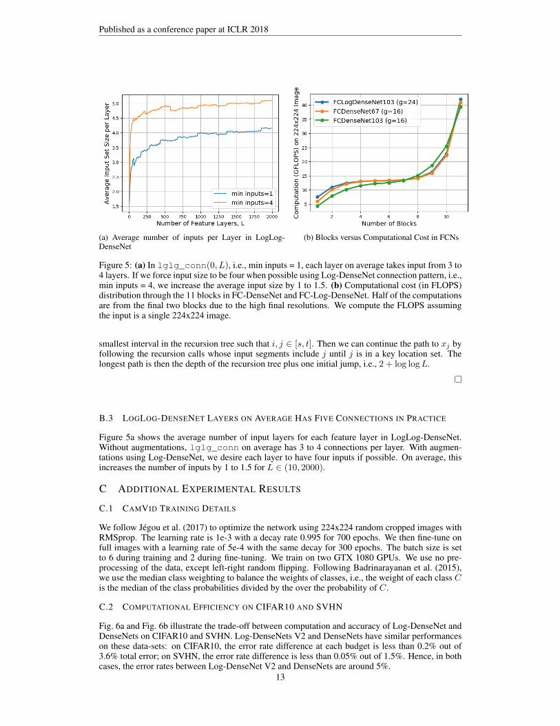
Figure 5: (a) In lglg_conn(0, L), i.e., min inputs = 1, each layer on average takes input from 3 to4 layers. If we force input size to be four when possible using Log-DenseNet connection pattern, i.e.,min inputs = 4, we increase the average input size by 1 to 1.5. (b) Computational cost (in FLOPS)distribution through the 11 blocks in FC-DenseNet and FC-Log-DenseNet. Half of the computationsare from the final two blocks due to the high final resolutions. We compute the FLOPS assumingthe input is a single 224x224 image.

smallest interval in the recursion tree such that i, j ∈ [s, t]. Then we can continue the path to xj byfollowing the recursion calls whose input segments include j until j is in a key location set. Thelongest path is then the depth of the recursion tree plus one initial jump, i.e., 2 + log logL.

B.3 LOGLOG-DENSENET LAYERS ON AVERAGE HAS FIVE CONNECTIONS IN PRACTICE

Figure 5a shows the average number of input layers for each feature layer in LogLog-DenseNet.Without augmentations, lglg_conn on average has 3 to 4 connections per layer. With augmen-tations using Log-DenseNet, we desire each layer to have four inputs if possible. On average, thisincreases the number of inputs by 1 to 1.5 for L ∈ (10, 2000).

C ADDITIONAL EXPERIMENTAL RESULTS

C.1 CAMVID TRAINING DETAILS

We follow Jegou et al. (2017) to optimize the network using 224x224 random cropped images withRMSprop. The learning rate is 1e-3 with a decay rate 0.995 for 700 epochs. We then fine-tune onfull images with a learning rate of 5e-4 with the same decay for 300 epochs. The batch size is setto 6 during training and 2 during fine-tuning. We train on two GTX 1080 GPUs. We use no pre-processing of the data, except left-right random flipping. Following Badrinarayanan et al. (2015),we use the median class weighting to balance the weights of classes, i.e., the weight of each class Cis the median of the class probabilities divided by the over the probability of C.

C.2 COMPUTATIONAL EFFICIENCY ON CIFAR10 AND SVHN

Fig. 6a and Fig. 6b illustrate the trade-off between computation and accuracy of Log-DenseNet andDenseNets on CIFAR10 and SVHN. Log-DenseNets V2 and DenseNets have similar performanceson these data-sets: on CIFAR10, the error rate difference at each budget is less than 0.2% out of3.6% total error; on SVHN, the error rate difference is less than 0.05% out of 1.5%. Hence, in bothcases, the error rates between Log-DenseNet V2 and DenseNets are around 5%.

13


(a) CIFAR10 Error versus FLOPS (b) SVHN Error versus FLOPS

Figure 6: On CIFAR10 and SVHN, Log-DenseNet V2 and DenseNets have very close error rates(< 5% relatively difference) at each budget.

(a) CIFAR10 Number of Parameters versus Er-ror Rates

(b) CIFAR100 Number of Parameters versus Er-ror Rates

(c) SVHN Number of Parameters versus ErrorRates

(d) ILSVRC Number of Parameters versus ErrorRates

Figure 7: The number of parameter used in the naıve implementation versus the error rates onvarious data-sets.

C.3 NUMBER OF PARAMETER VERSUS ERROR RATES.

Figure 7 plots the number of parameters used by Log-DenseNet V2, DenseNet, and ResNet versusthe error rates on the image classification data-sets, CIFAR10, CIFAR100, SVHN, ILSVRC. Weassume that DenseNet and Log-DenseNet use naıve implementations.

14


(a) LogLog-DenseNet Hub Multiplier=1 (b) LogLog-DenseNet Hub Multiplier=3

Figure 8: Performance of LogLog-DenseNet (red) with different hub multiplier (1 and 3). Largerhubs allow more information to be passed by the hub layers, so the predictions are more accurate.

C.4 LOGLOG-DENSENET EXPERIMENTS AND MORE PRINCIPLES THAN MBD

This section experiments with LogLog-DenseNet and show that there are more that just MBD thataffects the performance of networks. Ideally, since LogLog-DenseNet have very small MBD, itsperformance should be very close to DenseNet, if MBD is the sole decider of the performance ofnetworks. However, we observe in Fig. 8a that LogLog-DenseNet is not only much worse thanLog-DenseNet and DenseNet in terms accuracy at each given computational cost (in FLOPS), itis also widening the performance gap to the extent that the test error rate actually increases withthe depth of the network. This suggests there are more factors at play than just MBD, and in deepLogLog-DenseNet, these factors inhibit the networks from converging well.

One key difference between LogLog-DenseNet’s connection pattern to Log-DenseNet’s is that thelayers are not symmetric, in the sense that layers have drastically different shortcut connection in-puts. In particular, while the average input connections per layer is five (as shown in Fig. 5a), somenodes, such as the nodes that are multiples of L

12 , have very large in-degrees and out-degrees (i.e.,

the number of input and output connections). These nodes are given the same number of channelsas any other nodes, which means there must be some information loss passing through such “hub”layers, which we define as layers that are densely connected on the depth zero of lglg_conn call.Hence a natural remedy is to increase the channel size of the hub nodes. In fact, Fig. 8b showsthat by giving the hub layers three times as many channels, we greatly improve the performanceof LogLog-DenseNet to the level of Log-DenseNet. This experiment also suggests that the layersin networks with shortcut connections should ensure that high degree layers have enough capacity(channels) to support the amount of information passing.

C.5 ADDITIONAL SEMANTIC SEGMENTATION RESULTS

We show additional semantic segmentation results in Figure 9. We also note in Figure 5b howthe computation is distributed through the 11 blocks in FC-DenseNets and FC-Log-DenseNets. Inparticular, more than half of the computation is from the final two blocks because the final blockshave high resolutions, making them exponentially more expensive than layers in the mid depths andfinal layers of image classification networks.

15


Figure 9: Each row: input image, ground truth labeling, and any scene parsing results at 1/4, 1/2,3/4 and the final layer.

16

Documents

LOG-D N : HOW TO SPARSIFY A DENSENET - arXiv