Embed Size (px)
Citation preview

Log Sampling Methods and Software for Stand and Landscape AnalysesLisa J. Bate, Torolf R. Torgersen, Michael J. Wisdom, Edward O. Garton, and Shawn C. Clabough
United States Department of Agriculture
Forest Service
Pacific Northwest Research Station
General TechnicalReportPNW-GTR-746July 2008

Authors
Lisa J. Bate is a research wildlife biologist, 389 LaBrant Road, Kalispell, MT
59901; Torolf R. Torgersen is a research entomologist (emeritus), 4910 Paisley
Place, Anacortes, WA 98221; Michael J. Wisdom is a research wildlife biolo-
gist, U.S. Department of Agriculture, Forest Service, Pacific Northwest Research
Station, Forestry and Range Sciences Laboratory, 1401 Gekeler Lane, La Grande,
OR 97850; Edward O. Garton is a professor, Fish and Wildlife Resources Depart-
ment, University of Idaho, Moscow, ID 83844; Shawn C. Clabough is a software
and Web developer, 686 Fairview Drive, Moscow, ID 83843.
Cover
Photos clockwise from top left: American marten in log (by Evelyn Bull); hollow
log (by Lisa Bate); salamander on log (by Lisa Bate); early-seral forest with logs
(by Lisa Bate).
The Forest Service of the U.S. Department of Agriculture is dedicated to the principle of multiple use management of the Nation’s forest resources for sustained yields of wood, water, forage, wildlife, and recreation. Through forestry research, cooperation with the States and private forest owners, and management of the National Forests and National Grasslands, it strives—as directed by Congress—to provide increasingly greater service to a growing Nation.
The U.S. Department of Agriculture (USDA) prohibits discrimination in all its programs and activities on the basis of race, color, national origin, age, disability, and where applicable, sex, marital status, familial status, parental status, religion, sexual orientation, genetic information, political beliefs, reprisal, or because all or part of an individual’s income is derived from any public assistance program. (Not all prohibited bases apply to all programs.) Persons with disabilities who require alternative means for communication of program information (Braille, large print, audiotape, etc.) should contact USDA’s TARGET Center at (202) 720-2600 (voice and TDD).
To file a complaint of discrimination, write USDA, Director, Office of Civil Rights, 1400 Independence Avenue, SW, Washington, DC 20250-9410 or call (800) 795-3272 (voice) or (202) 720-6382 (TDD). USDA is an equal opportunity provider and employer.

Abstract
Bate, Lisa J.; Torgersen, Torolf R.; Wisdom, Michael J.; Garton, Edward O.;
Clabough, Shawn C. 2008. Log sampling methods and software for stand and
landscape analyses. Gen. Tech. Rep. PNW-GTR-746. Portland, OR: U.S. Depart-
ment of Agriculture, Forest Service, Pacific Northwest Research Station. 93 p.
We describe methods for efficient, accurate sampling of logs at landscape and stand
scales to estimate density, total length, cover, volume, and weight. Our methods
focus on optimizing the sampling effort by choosing an appropriate sampling
method and transect length for specific forest conditions and objectives. Sampling
methods include the line-intersect method and the strip-plot method. Which method
is better depends on the variable of interest, log quantities, desired precision, and
forest conditions. Two statistical options are available. The first requires sampling
until a desired precision level is obtained. The second is used to evaluate or monitor
areas that have low log abundance compared to values in a land management plan.
A minimum of 60 samples usually are sufficient to test for a significant differ-
ence between the estimated and targeted parameters. Both sampling methods are
compatible with existing snag and large tree sampling methods, thereby improving
efficiency by enabling the simultaneous collection of all three components—snags,
large trees, and logs—to evaluate wildlife or other resource conditions of interest.
Analysis of log data requires SnagPRO, a user-friendly software application
designed for use with our sampling protocols. Default transect lengths are sug-
gested for both English and metric measurement systems, but users may override
default values for transect lengths that better meet their specific sampling designs.
SnagPRO also analyzes wildlife snag and large tree data.
Keywords: Coarse woody debris, density, down woody material, line intersect,
logs, monitoring, percent cover, sampling technique, snag, large tree, SnagPRO,
strip plot, total length, volume, weight, wildlife management, wildlife use.

Contents 1 Introduction
5 General Information
5 About SnagPRO
6 Files Online
6 Sampling Applications
7 Methods
7 Sampling Objectives (Step 1)
8 Landscape Definition and Selection (Step 2)
8 Landscape Stratification (Step 3)
9 Stratify the Survey Area
11 Choosing the Appropriate Sampling Method: LIM, SPM, or Both (Step 4)
17 Establishing Transects (Step 5)
20 Field Techniques (Step 6)
26 SnagPRO Analysis (Step 7)
44 Wildlife Use Signs
45 Tutorials
45 Example I: Metric Weight and Density Estimates for a Single Stand Using LIM and SPM Tally
53 Example II: English Parameter Estimates and Statistical Test for a Stratified Landscape Using SPM
65 Example III: Metric Parameter Estimates for a Stratified Landscape Using a Combination of LIM and SPM
75 Acknowledgments
75 English Equivalents
76 References
81 Appendix 1: Customized Log Measuring Sticks
83 Appendix 2: LIM Field Form Explanations
86 Appendix 3: SPM Field Form Explanations
90 Appendix 4: General Instructions for Analysis Within a Single Stratum
92 Appendix 5: General Instructions for Analysis Within a StratifiedLandscape

Log Sampling Methods and Software for Stand and Landscape Analyses
1
Introduction
It is the natural fate of standing trees and snags to become part of the wood com-
ponent on the forest floor. Individual branches, tops, or whole trees are recruited to
the forest floor through a variety of natural processes such as lightning, snow, and
wind. Other natural processes such as the activity of insects and disease that kill
or physically weaken trees likewise contribute dead wood to the forest floor. Insect
outbreaks, windstorms, avalanches, floods, and fires can result in large accumula-
tions of downed wood in concentrated areas.
Down woody material (DWM), in the form of natural and cut logs, is a critical
resource with multifaceted functions in forested ecosystems. For example, DWM
provides a reservoir of minerals, nutrients, and moisture for establishment of tree
seedlings (Harmon and others 1986), reduces soil erosion, and contributes to soil
productivity (Harvey and others 1987, Jurgensen and others 1997). Fire behavior,
management, and smoke production are substantially affected by the abundance,
distribution, and size of DWM (Brown 1974, Sandberg and Ottmar 1983, Walstad
and others 1990). Many wildlife species depend on logs as habitat (Bartels and
others 1985, Bull and others 1997, Franklin and others 1981, Lofroth 1998, Maser
and others 1979, Mellen and others 2006). Logs function as a foraging substrate for
many wildlife species (Carey and Johnson 1995, Tallmon and Mills 1994, Torg-
ersen and Bull 1995). Other species use logs for thermal and hiding cover (Bull
and others 1997, Maser and others 1979). In addition, hollow logs serve as sites for
denning, resting, and hibernation for a number of large and small mammals (Bull
and others 1997). Thus, dead wood in all its forms is a fundamental feature of
healthy forests.
The “life” or persistence of logs, especially large ones, can last several decades
or even a century (Bull and others 1997). For both plants and animals, down wood
in all forms represents a rich substrate on which to feed and live. Insect-eating,
fungus-eating, wood-eating, and predaceous animals find rich and varied sources
of food associated with logs. Logs protect wood-dwelling organisms with moist,
thermally stable, predator-protected niches. From microscopic protozoa and fungi
to birds and small mammals, down wood teems with life. Many of these organisms
are connected by functional pathways that are partially or completely unknown.
Logs provide a complex structure where animals find stable temperatures and
moisture for nesting, denning, feeding, and food storage. The size (diameter and
length) of logs is a key indicator of their use and value to wildlife. Smaller logs
benefit small mammals, amphibians, and reptiles, for which they function primari-
ly as escape cover and shelter when the animal can get inside or under the log (Bull
and others 1997). Large logs, especially hollow ones, are an especially important

GENERAL TECHNICAL REPORT PNW-GTR-746
2
structure in forested ecosystems, and their retention has been strongly emphasized
(Bull and others 1997, Mellen and others 2006). Marten (Martes americana),
mink (Mustela vison), coyote (Canis latrans), bobcat (Felis rufus), cougar (Felis
concolor), and black bear (Ursus americanus) all will use hollow logs for denning,
hibernation, shelter, and resting. Research on fisher (Martes pennanti) suggests
that up to three dens may be used in rearing a litter. Although most dens are in
cavities high in large living or dead trees, large logs also are used (Powell and
Zielinski 1994).
Hollow logs do not develop from solid logs, but instead develop their hollow
characteristics as living trees. Live trees that are injured in such a way that their
heartwood comes into contact with heartrot fungi (for example, broken branch,
broken top, or fire scar), slowly develop heartrot (decay of the heartwood). Once
infected, the tree does not die but continues to grow even though portions of
the heartwood soften. Over time, the decay may become so extensive that the
heartwood falls and internal hollow pockets are formed. Eventually, these hollow
trees become snags and then fall over to become hollow logs, a critical resource in
forested ecosystems (Bull and others 1997).
Logs in all stages of decay provide foraging opportunities for a variety of
wildlife species. During late summer and fall, bears forage on invertebrates in large
logs. Bull and others (2001) found that log-associated insects composed a large por-
tion of the diet of black bears. Pileated woodpeckers (Dryocopus pileatus) also feed
extensively on insects in large logs (Bull and Holthausen 1993, Torgersen and Bull
1995). Most of these logs are in the advanced stages of decay. In addition, Picoides
woodpeckers will feed on beetle larvae found in sound logs that have recently died.
Small mammal populations are positively associated with cover of logs, which
provide not only needed cover but also hypogenous fungi for foraging (Carey and
Johnson 1995, Tallmon and Mills 1994). Small mammals also use logs extensively
as runways (Hayes and Cross 1987). Logs in or near streams, ponds, or lakes
provide structure for amphibians, beaver (Castor canadensis), mink, otter (Lutra
canadensis), and birds and for both passage within and across waterways. In turn,
small mammals are prey for reptilian, avian, and mammalian predators (Carey and
Johnson 1995). Hence, predators are also associated with log abundance. A study
conducted on great gray owls (Strix nebulosa) found that prey captures were within
1 m (3 ft) of downed wood 80 percent of the time (Bull and Henjum 1990).
Large numbers of down trees can form a maze of logs, many of which can be
100 cm or more above the ground. Patches of these jackstrawed logs often are found
in mature stands and provide critical structure for many animals. Marten, mink,
and cougar hunt in them; when snow covers the logs, a complex array of snow-free
Log Sampling Methods and Software for Stand and Landscape Analyses
3
spaces and runways provide important habitat under the snow for protection and
foraging by marten, fisher, and small mammals (Bull and others 1997). In north-
central Washington, lynx (Lynx canadensis) frequent Englemann spruce/subalpine
fir/lodgepole pine (see appendixes for species names) stands with high densities of
jackstrawed logs 30 to 122 cm above the ground, which are used for denning and
hunting (Koehler and Aubry 1994). Tree squirrels (Sciurus spp.) also spend much
of the winter in this environment, where they feed on seeds from cached cones.
Logs also serve as sunning and lookout posts. Spruce grouse (Dendragapus
canadensis) regularly sit on logs, where they apparently are better able to avoid
predation (Bull and others 1997). In spring, males use these elevated sites as
walkways for their displays.
For fire managers, however, logs can be a resource of concern because of their
fire potential. Since the early 1900s, active fire suppression has been a priority in
forest management (Norris 1990). This has resulted in high fuel loads across cer-
tain landscapes, leading to high-severity fires. Consequently, down wood surveys
to estimate log volume or weight often are conducted to determine fire potential
(Brown 1974, Fischer 1981) and to assess whether management actions, such as
thinning, prescribed burning, or log removal, should occur.
Despite the importance of logs to many resource disciplines, methods for
sampling logs have focused almost exclusively on silvicultural or fire applications.
Warren and Olsen (1964) first presented line-intersect theory and technique for
sampling logging residue in harvested stands. De Vries (1973) later expanded on
the theory of line-intersect sampling, finding that given a large number of intersec-
tions, this technique could be used to obtain estimates of several log variables.
Soon after, Brown (1974) presented the planar-intersect technique. Brown’s method
was developed to estimate volume and weight of down woody fuels to help re-
source specialists manage fuels and predict fire behavior. Although termed differ-
ently, both the line- and planar-intersect methods have the same theoretical basis
and use the same equations (Brown 1974, De Vries 1973).
Line-intersect methods (LIM) were designed primarily to estimate wood
volume or weight, but other variables such as cover may be more meaningful for
wildlife and other resources. DecAID—a snag, decayed tree, and down wood ad-
visory tool—recommends using percent cover to characterize down wood used by
wildlife (Mellen and others 2006). DecAID is designed to help managers evaluate
forest conditions and the effects of management on organisms that use snags and
down wood.
Log density and length also are important variables that affect wildlife use. To-
tal length of logs, for example, was used to describe the foraging habitat of pileated
Despite the
importance of logs
to many resource
disciplines, methods
for sampling logs
have focused almost
exclusively on
silvicultural or
fire applications.

GENERAL TECHNICAL REPORT PNW-GTR-746
4
woodpeckers (Bull and Holthausen 1993, Torgersen and Bull 1995). Density of logs
of specific diameter and length often are used as a guideline for managing wild-
life habitat in forest plans (USDA Forest Service 1995). Consequently, given the
diverse number of log variables of interest to multiple disciplines, understanding
log sampling methods and their strengths and weaknesses is essential to effective
use and applications.
The LIM has been shown to be an unbiased method for sampling log volume in
tractor- or cable-logged stands (Hazard and Pickford 1978, 1986). It is also an effi-
cient sampling method for estimating total length of logs, percentage of cover (also
referred to as percent cover or cover), volume, and weight in areas of relatively high
log abundance with normally distributed lengths and diameters (Bate and others
2004). For variables such as log density, however, the strip-plot method (SPM), or
area-plot sampling, is more precise and efficient. Furthermore, in areas where logs
are scattered and low in abundance, the SPM often yields a more precise estimate
with less sampling effort in contrast to LIM. Levels of use by certain guilds of
wildlife (for example, woodpecker foraging, squirrel middens) may also be evalu-
ated by using SPM.
Our paper is intended to serve as a guide for log sampling, from the early steps
of establishing study sites through field methods and data analyses. Our protocols
provide methods to sample logs accurately and efficiently at stand or landscape
scales. Methods can be used to conduct research, to monitor compliance with
management guidelines or prescriptions, or to monitor the effectiveness of manag-
ing logs for wildlife or other resources.
Our methods have particular utility in helping integrate silviculture, fire, wild-
life, and soils programs to simultaneously consider all of these resource disciplines
in research or management, while maximizing sampling efficiency. Estimates can
be considered among all disciplines to evaluate resource tradeoffs and integrate
management. Given the small budgets typically available for forest sampling and
inventory, use of accurate and efficient methods of sampling logs, such as those
described here, provides essential support for research and management of logs and
associated resources.
Included are instructions for downloading the SnagPRO software application
(Bate and others, in press) for designing surveys and analyzing data. Sampling
methods focus on optimizing sampling effort by choosing an appropriate sampling
method for the specific conditions encountered in relation to objectives. Sampling
methods include LIM, SPM, or a combination. Choice of method will depend
on the variables of interest, abundance of logs in the size and condition (decay
attributes) of interest, desired precision, and forest conditions. We provide a

Log Sampling Methods and Software for Stand and Landscape Analyses
5
dichotomous key to help users select the best log sampling method to meet
their objectives.
General Information
About SnagPRO
SnagPRO (Version 1.0) software analyzes log abundance based on peer-reviewed,
scientific sampling protocols. It was specifically developed to analyze log data
following the sampling protocols presented in this report, as well as snag and large-
tree sampling protocols developed in a companion publication (Bate and others,
in press). Logs can be sampled using one of two sampling methods: (1) the line- or
planar-intersect method (Brown 1974, De Vries 1973); or (2) the strip-plot method
(Bate and others 2004). In some situations—diverse type and number of logs
among strata, for example—it may be more efficient to use a combination of both
methods. SnagPRO also provides this option. Log variables include density, total
length, cover, volume, and weight. SnagPRO provides estimates of these log charac-
teristics from use of either sampling method, expressed in English or metric units.
SnagPRO allows users to determine the optimal transect length within an area
by analyzing a small sample of preliminary data, referred to as a pilot sample. Log
abundance and distributions vary considerably across landscapes. Consequently,
analysis of pilot samples to optimize sampling design and effort is an important,
early step in field sampling.
Identifying the optimal transect length is accomplished by sampling along
a standardized transect length composed of eight subsegments. For metric users
this is a 100-m transect length divided into eight 12.5-m subsegments. For English
users, a 400-ft transect length divided into eight 50-ft subsegments. SnagPRO can
then divide transects into four lengths and calculate the mean and variance of each.
The length that minimizes the variance—and therefore the sample size required—
is considered the optimal transect length.
Resource specialists may customize log surveys to meet their specific needs
while adhering to the general protocol suggested here. Default transect lengths
can be overridden to meet specific objectives. For simplicity, our paper focuses on
default transect lengths. Resource specialists may also use SnagPRO for analyses
of snags and trees, based on additional sampling protocols and analysis procedures
designed for these structures (Bate and others, in press).
Two statistical options are available for analysis. The first requires sampling un-
til a desired precision is obtained. The second is used for compliance monitoring in
areas that have low log abundance compared to values in a land management plan
SnagPRO allows
users to determine
the optimal transect
length within an area
by analyzing a small
sample of preliminary
data, referred to as a
pilot sample.
The length that
minimizes the
variance—and
therefore the sample
size required—
is considered the
optimal transect
length.

GENERAL TECHNICAL REPORT PNW-GTR-746
6
(LMP). With a minimum of 60 samples, users may test for a significant difference
between the estimated and targeted parameters.
Files Online
Download SnagPRO from the USDA Forest Service Pacific Northwest (PNW) Web
site at http://www.fs.fed.us/pnw/publications/gtr746/index.shtml. The SnagPRO
installation requires at least 5 MB of space. SnagPRO requires another 10 to 50 MB
of space to operate.
Users may choose where to install SnagPRO, although the default location is
in C:\Program Files. Once installed, users may create a shortcut to SnagPRO for
their desktops or Quick Launch bar. Once installed, double-click the icon to launch
SnagPRO, or launch directly from the executable file, SnagPRO.exe file.
Two Microsoft Excel files—LIMdata.xls and SPMdata.xls—are included in
the zipped SnagPRO file. Each file contains multiple worksheets. Three files in
the LIMdata.xls and two in the SPMdata.xls contain sample data sets for use with
the tutorials found at the end of our paper. One worksheet contains a sample data
form that can be printed for use in the field (Field Form). The final worksheet is
for resource specialists who want to enter their data directly into a spreadsheet file
while in the field (Data Entry). Remember, database users can do the same, but need
to format their data as shown in the examples below before importing to SnagPRO.
A text file for each method provides the explanations needed for using field forms.
These forms can easily be modified for specific sampling needs.
Existing resource data—stored in spreadsheet or database—must be correctly
formatted as a comma-separated-value (CSV) file before importing to SnagPRO.
For simplicity, our paper addresses only spreadsheet examples, and data files for the
tutorial are in spreadsheet format.
Sampling Applications
Our methods and the supporting SnagPRO software were designed to guide the
choice of sample design, sampling methods, and types of analyses to produce
reliable and efficient results for research or management applications with minimal
sampling effort and analysis time. We designed these sampling techniques to
address the needs of wildlife resource specialists, but they are also appropriate
for other disciplines such as silviculture, fire, and soils. Our techniques may also
complement the data collected in other projects (for example, project planning,
effects analyses, stand exam, or Forest Inventory Analysis [FIA] data) by convert-
ing the data sets to similar units of measurement (e.g., number/ac [number/ha]) to
provide additional baseline data for resource specialists.

Log Sampling Methods and Software for Stand and Landscape Analyses
7
Recommendations here are based on a log sampling study conducted in
mixed-conifer forests within the Columbia River basin (CRB) region, specifically
Oregon and Montana (Bate and others 2004). This study investigated the accuracy,
precision, and efficiency of the LIM and SPM for sampling log resources important
to wildlife.
Methods
Sampling Objectives (Step 1)
Most ecological studies are designed to answer some form of the question: How
many are there? For example, do silvicultural practices comply with management
guidelines for log density? Or, what is the difference in log cover in areas used
for lynx dens compared to areas that are not? Accordingly, the first step in any
sampling program is to specify the sampling objective(s). User’s objectives
ultimately determine the amount of time and resources needed to obtain estimates
with a desired level of precision. Objectives can be clarified by answering the
following questions:
1. What log sizes (diameter and length) are of interest?
2. Which variables are of interest—density, total length, percentage cover,
volume, or weight?
3. Will data be used to check compliance with management guidelines, to es-
tablish baseline data for monitoring, or to assess habitat for a threatened or
endangered species? This answer often dictates the answers to the follow-
ing questions.
4. How precise do users need their estimate?
5. Is log species important? If so, why?
6. Are data on wildlife use of logs important (for example, woodpecker for-
aging, squirrel middens)?
As Krebs (1989) stated, “Not everything that can be measured should be.”
Time spent on extraneous data collection limits the number of samples and the
subsequent results. For example, identifying each log by species seems simple. Yet,
species identification can often substantially increase the amount of survey time,
especially for inexperienced field crew members. Therefore, users should specify
their objectives and how data will be used before starting log surveys.
As a general guideline for acceptable precision, we recommend sampling
sufficient to estimate parameters within 20 percent of the true mean, 90 percent of
the time. These values are set as defaults in SnagPRO. We have observed that when
logs are relatively rare and have clumped distributions, the required sample sizes to
GENERAL TECHNICAL REPORT PNW-GTR-746
8
gain a higher level of precision (for example, within 10 percent of the true mean, 95
percent of the time) often are cost and area prohibitive. Only when logs are abun-
dant and randomly distributed would higher precision be manageable.
Landscape Definition and Selection (Step 2)
The second step is to define the landscape by delineating the boundaries of the
sampling area. Our methods were designed to be compatible with the snag and
large tree sampling methods developed by Bate and others (1999a, in press). Meth-
ods for sampling snags and large trees were initially developed on landscapes of
1200 to 2800 ha (3,000 to 6,900 ac) (Bull and others 1991). Log sampling methods
can also be used on a subwatershed scale with a few modifications. See “Establish-
ing Transects” and “Compare to Target” sections for details.
Subwatersheds in the CRB range from about 160 to 8100 ha (400 to 20,000 ac)
(Quigley and others 1996). The sampling area for logs, however, need not be a sub-
watershed or other large landscape. Our methods may also be used for individual
stands (<40 ha or 100 ac), or a group of stands, given that the log size of interest is
relatively abundant. If the logs of interest are relatively rare (e.g., <100 to 150/ha) in
small stands used as sample units, a complete count may be more appropriate.
Landscape Stratification (Step 3)
Perhaps the most important step is the stratification process. Although the initial
investment of time may seem large, appropriate stratification will ultimately reduce
sampling effort and increase precision (Krebs 1989). Stratification often can be
based on strata established for prior silvicultural or inventory work. For example,
many foresters stratify the landscape to conduct stand exams, and their delinea-
tions may work well for sampling logs. If log sampling occurs with snag sampling,
stratification based on snag abundance is more appropriate. Obtaining precise
estimates of snag conditions often is more difficult than for logs, owing to the lower
abundance of snags and higher variability of estimates.
The need to stratify the landscape as part of sampling depends on several
factors (Cochran 1977):
• Stratification may increase precision of estimates. If, for example, the
landscape has distinct areas of high versus low log abundance, estab-
lishing corresponding strata of high or low abundance can substantially
improve precision and reduce the sampling effort required to obtain the
desired precision.
Although the
initial investment
of time may seem
large, appropriate
stratification will
ultimately reduce
sampling effort and
increase precision.

Log Sampling Methods and Software for Stand and Landscape Analyses
9
• Sampling problems can differ spatially according to forest community
type, timber harvest method, or seral stage, and stratification of these con-
ditions can often increase precision.
• Resource specialists may want to obtain separate estimates for
management-based subdivisions of the landscape. For example, part of
a subwatershed may be managed for timber production and another part
may be managed as a research natural area.
If one or more of the above criteria applies to the situation, it would probably be
beneficial to stratify. SnagPRO can accommodate up to four strata. If the landscape
is homogeneous throughout in regard to log abundance and forest structure, there is
probably little to be gained by stratifying.
Stratify the Survey Area
Use the following steps to stratify the survey area:
1. Visit the area first, as landscape patterns become apparent from an initial
ground survey. Ask, “What differences and similarities in log abundance
and vegetative structure are evident across the landscape?”
2. Obtain reference maps for field use, such as geographic information sys-
tem (GIS) maps, U.S. Geological Survey (USGS) orthoquad maps, or both.
Request metadata (data definitions) for maps and data. Maps should dis-
play the following necessary information:
a. Road system with road type and maintenance level.
b. Stand or vegetation units and their respective unique numeric identifiers.
c. Current seral stage of vegetation at 1:31,680, or less.
3. Query databases to obtain the following information about each stand: for-
est type (low versus high elevation, dry versus moist), management activi-
ties, seral stage, disturbance history (wind, fire, insects, and disease) and
any other factors that may affect log abundance. Make sure the data report
includes types of management activities, such as harvest method used,
slash and burn prescriptions, thinning, and management direction for
log retention.
4. Check the map and stand data using aerial photographs. Generally, the
amount of time spent stratifying the stands in the field is inversely propor-
tional to the quality of the original stand data collected or the quality of
the data query. Review the metadata before heading to the field.
5. Revisit the survey area with the field maps. Plan to spend at least one day
to validate the information on the map(s) and data report.

GENERAL TECHNICAL REPORT PNW-GTR-746
10
6. Assign each stand to a stratum. Estimate the number of hectares (acres)
within each stand or stratum.
Most landscapes targeted for log sampling have undergone some timber
harvest. Consequently, depending on the method of harvest, the placement of each
stand within a stratum may or may not be straightforward. For example, most
unharvested mature/old-growth stands in mixed-conifer forests have an abundance
of logs. By contrast, older harvest units that had been clearcut and broadcast
burned may have few logs. Finally, more recent clearcuts may have logs uniformly
distributed, reflecting policy changes.
For old growth or clearcut harvest situations, combine all unharvested ma-
ture/old-growth stands into a single stratum. Then consult silviculturists, query
databases, and conduct a ground check to determine when log retention began in
harvest units. Place older clearcut stands that had no management guidelines for
logs in one stratum, and more recent clearcut areas in another stratum. Generate
a new map of all stands categorized as one of three strata: (1) recent clearcut, (2)
older clearcut, and (3) unharvested mature/old growth.
Establishing the strata is more time-consuming for areas of selection harvest,
especially if GIS stand data are unavailable. In this situation, visit individual
stands to examine log abundance and stratify accordingly. Furthermore, unlike the
stratification process for snags or large trees, which often can be done quickly by
viewing small portions of the stand’s edge (Bate and others 1999a), the stratifica-
tion process for logs typically requires more thorough stand reconnaissance. This
is because fuelwood gathering, wind effects, diseases, and insects can dramati-
cally alter the patterns of log abundance along the edge of a stand compared to the
interior. Furthermore, both grass and shrub cover near stand edges can obscure
smaller logs from sight.
The manner in which a watershed or other landscape is stratified is dictated by
the sampling objectives. How does the log size of interest vary in abundance across
the sampling area? If the main objective is to obtain density estimates of large
(>25 cm [10 in] large-end diameter [LED]) logs, stratification is dictated solely by
this LED size class. Stands with high densities should be placed together in one
stratum; stands with low densities should be placed in another. If precise estimates
of both small and large logs are desired, such as for log sampling to assess fuel
loadings (smaller logs) and wildlife habitat (larger logs), stratification should be
based on whether small or large size classes of logs are more variable. If snags and
trees also are sampled, stratification should be based on the component for which it
is considered most difficult to obtain a precise estimate. Usually, this is snags.
Log Sampling Methods and Software for Stand and Landscape Analyses
11
Another criterion for landscape stratification is seral stage or method of past
timber harvest, which may affect the level of difficulty in conducting the survey.
Dense shrub or seedling/sapling densities can make it difficult to sample accurately
with the SPM for variables other than log density.
Finally, stratification of landscapes often is dictated by differences in land
management use. If separate estimates are needed for areas that are managed for
different purposes (for example, riparian areas versus high-production timber
areas), stratification based on these different land allocations is needed.
Standstratification—
Stands, by definition, are homogeneous units and usually should not require strati-
fication. An exception may be large mature or old-growth stands surrounded by
stand-regenerating harvests. Trees along the edges of these older stands are more
susceptible to blowdown, creating well-defined borders of high log abundance in
contrast to interior parts of the stand. In this case, the edge should be treated as
its own stratum. Otherwise, the variance within the stand may be so great that it
becomes difficult to obtain a precise estimate.
Choosing the Appropriate Sampling Method: LIM, SPM, or Both (Step 4)
The log characteristics to be sampled affect the choice of sampling method. Density
is the number of logs per hectare or acre. Total log length is the combined length of
logs per unit area (either m/ha or ft/ac). Cover is the percentage of ground covered
by logs. This can be calculated by treating each log as a trapezoid and determin-
ing what percentage of the ground is covered with these trapezoid-shaped areas.
Volume of logs is cubic meters of logs per hectare or cubic feet per acre. Weight is
the metric tons of logs per hectare or tons per acre.
The LIM is based on probability sampling (De Vries 1973). To obtain estimates
of each variable, specific measurements of intersected logs (diameter and/or length)
are taken (fig. 1a). These measurements are then inserted into equations unique
to each variable to obtain estimates (De Vries 1973). Only logs whose central
axis is intersected by a transect line are measured (Brown 1974). Approximately
100 intersections are needed to obtain a reasonably precise estimate of weight or
volume within a given area (Brown, J.K. 1998. Personal communication. Retired
research forester, USDA Forest Service Rocky Mountain Research Station). Table
1 describes the log measurements and data required for estimates of each variable
using LIM. See formulas in the “Computer Analysis” section for each equation.
By contrast, the SPM is a type of area-plot sampling. “Strip plot” refers to plots
that are long and narrow rectangles (Husch and others 1972). Estimates using SPM
The log
characteristics
to be sampled
affect the choice
of sampling
method.

Figure 1—Field measurements necessary to obtain estimates of all log parameters using the LIM (A) and SPM (B). In addition, the condition of each log (sound or rotten) is required to estimate weight.
GENERAL TECHNICAL REPORT PNW-GTR-746
12
are obtained by first taking the necessary log measurements within the area of a
strip plot (fig.1b and table 1), and then converting this to hectares or acres. For our
methods, the default area for a metric strip plot is 50 m2 (4 m wide by 12.5 m long),
centered on a transect line (fig. 1b). For English units, the default area is 600 ft2
(12 ft wide by 50 ft long), centered on a transect line. Table 1 contains the required
information about each log for estimates of each variable when using SPM. See
formulas in the “Computer Analysis” section for each equation.
Outer strip-plot boundaries are determined by using a meter- or 3-ft caliper
(fig. 2a and 2b) or a customized measuring stick (see appendix 1 for details), which
functions as a square. The rectangular shape of the strip plot was selected because
rectangles, in contrast to other plot shapes, reduce the sampling variance of logs
and other forest structures that often are distributed in clumps (Krebs 1989,
Warren and Olsen 1964). A 4-m or 12-ft width was used because this width

Figure 2—Calipers function as a square when using strip-plot method (A). Two lengths of the calipers denote the outer boundaries of the plot and the place to where the length is measured and the large (or small) diameter is taken (B).
A
B
Log Sampling Methods and Software for Stand and Landscape Analyses
13
typically is sufficient to sample logs, and is narrow enough to avoid the need
for laying out additional plot boundary lines (Bate and others 2004).
The first consideration in choosing a sampling method is the log variables
of interest. Table 2 provides general guidelines for the decisionmaking process.
For example, if only log density is of interest, the choice is easy: use SPM. It is
more precise and takes less than half the time to implement in the field (Bate
and others 2004). If variables other than density are desired, then other factors
become important.
Second, consider the density of logs present. During the stratification process,
an ocular assessment of log density by size class is first done as part of initial site
visits. If logs appear to be relatively rare, use SPM. If the logs are so numerous as
to be arranged in jackstraw piles and density is not a variable of interest, LIM is
preferable. See table 2 for general guidelines.
Third, consider the stand characteristics. Has timber harvest occurred? In
unharvested stands, the lengths and diameters of logs intersected when using LIM
tend to be normally distributed, with midlength and middiameter logs being the
most common logs (Bate and others 2004). In these situations, LIM yields precise
and accurate estimates. In some types of harvested stands, however, most logs tend
to be short and small in diameter, with few logs present that are long and large in
Table 1–Field measurements required to obtain estimates offivelogvariablesbyusingtheline-intersect(LIM)orstrip-plot(SPM)methoda
Field measurement required
Variable LIM SPM
Density Log length Endpoint (LED) in or out?
Total length Number of log intersections
Length of log within strip plot
Percent cover Diameter at intersection
Length, small- and large-end diameters within strip plot
Volume Diameter at intersection
Length, small- and large-end diameters within strip plot
Weight Diameter at intersection and condition
Length, small- and large-end diameters within strip plot, and condition
a For analysis by size class, the large-end diameter (LED) also needs to be recorded for all variables.

GENERAL TECHNICAL REPORT PNW-GTR-746
14
diameter. In this latter situation, it may be difficult to obtain precise estimates with
LIM because of the high variance in log characteristics. Consequently, SPM
is likely a better choice.
Fourth, consider the landscape conditions. How easy or difficult would it be
to travel from one point to another to establish sampling transects? The process
of locating and establishing sampling transects takes substantially more time than
sampling. This is especially true for landscape analyses. Establishment of transects
using SPM takes about one to four times as much time as actual sampling. For LIM,
Table 2–Dichotomous key for selecting initial sampling method within a stratum based on log variables desired
1 Density is the only desired variable; log abundance low to high; unharvested or harvested stands ................................................................................................................SPM
1 Percentage cover, volume, weight, total length of logs; unharvested or harvested stands 2*
1 All variables; unharvested or harvested stands ..................................................................3*
2 Log abundance High; >11 logs intersected per 100 m of transect .................................. LIM
2 Log abundance Moderate; 6-11 logs intersected per 100 m ..................................................4
2 Log abundance Low; <6 logs intersected per 100 m ......................................................SPM
3 Log abundance High; >11 logs intersected per 100 m of transect ......... LIM and SPM Tally
3 Log abundance Moderate; 6-11 logs intersect per 100 m ......................................................5
3 Log abundance Low; <6 logs intersected per 100 m ......................................................SPM
4 Stands or landscapes with relatively light ground cover in the form of shrubs or young trees; sampling or travel not likely to be impeded by such ground cover ...........SPM
4 Stands or landscapes with ground cover dominated by shrubs or young trees that will likely impede sampling or travel ....................................................................... LIM
5 Stands or landscapes with relatively light ground cover in the form of shrubs or young trees; sampling or travel not likely to be impeded by such ground cover .............SPM
5 Stands or landscapes with ground cover dominated by shrubs or young trees that will likely impede sampling or travel ................................................... LIM and SPM Tally
* Users should be aware that in harvested stands composed of mainly short log lengths and small diameters with only a few large logs, the SPM may be a better choice for sampling owing to the high variance associated with LIM sampling in these conditions.

Figure 3—When the line-intersect method is used, diameters of qualifying logs are measured where the transect line intersects the central axis of the log.
Log Sampling Methods and Software for Stand and Landscape Analyses
15
establishment takes about three to six times as long. Although it generally takes
less time per unit transect sampled with LIM (obtaining density estimates being the
only exception), less information is also collected per unit transect. This translates
into larger sample size requirements to obtain desired precision (Bate and others
2004). Therefore, if a large amount of time is anticipated to locate and establish
transects, owing to steep terrain or limited access, SPM is the better choice, given
that sampling conditions are not hampered by a high abundance of logs or
shrub cover.
High shrub cover causes difficult traveling and sampling condi-
tions. In areas where shrubs are so dense that taking measurements of
log lengths within the strip-plot boundaries is difficult, LIM is likely
a better choice. This is true unless log abundance is too low to obtain
a reasonably precise estimate with the LIM or log density is the only
variable of interest.
Users are not limited to using SPM or LIM exclusively. There may
be cases when doing so results in an unnecessary amount of field effort.
For example, in areas of high log abundance with multiple variables
of interest, it may be beneficial to use a combination of SPM and LIM
(see example I in the “Tutorial” section for details). Use the LIM to estimate total
log length, percentage cover, volume, and weight (figs. 3 and 4). Use the SPM to
estimate log density from a tally of endpoints of logs within 2 m of the transect
line used for LIM (fig. 4). The advantage with this approach is that field observers
need not leave the centerline to make measurements in difficult field conditions.
The disadvantage is that field assistants need to be trained to sample logs using two
methods.
The other situation where a combination of the two methods is beneficial is on
a landscape that needs to be stratified because of high variability in log density.
For example, if density in one area is extremely high, making travel and sampling
difficult, LIM is the better method for estimating log volume. In areas that have
undergone timber harvest and have low log density, SPM is a better choice. Then,
using a special section called Combo within SnagPRO, a stratified estimate of log
volume can be obtained. The only unique aspect of this file is that all parameter
estimates need to be converted to acres or hectares before this utility is used. See
Example 3 in the “Tutorial” section for details.
Classifyinglogsbysize(LED)—
Just as snags and trees are categorized by their diameter at breast height (d.b.h.),
logs are best categorized by their LED. For logs with rootwads intact, the LED is
equivalent to the d.b.h. if the tree had remained standing (fig. 5). For logs with no
Just as snags
and trees are
categorized by their
diameter at breast
height (d.b.h.), logs
are best categorized
by their LED.

Figure 4—Combination of log sampling techniques: Line-intersect method (LIM) and strip-plot method (SPM) tally. Two logs qualify for the LIM because their central axes are intersected by the central tran-sect line. Three logs qualify for the the SPM tally because their LEDs lie within 2 m of the central transect line.
GENERAL TECHNICAL REPORT PNW-GTR-746
16
rootwad attached, the LED is the diameter
at the largest end of the log that is complete
(fig. 5).
Large-end diameters define a log
population and allow for accurate temporal
and spatial comparisons of logs among
size classes. In the past, most log sampling
techniques required data only on the
diameter of a log at the point of intersection.
This greatly limited the value of the data for
wildlife specialists, because often only the
larger logs are of interest. For example, two
stands may have the same volume of logs.
What cannot be determined, unless LED
is recorded, is whether logs are small and
numerous or large and uncommon. Further-
more, setting a high minimum diameter for
logs to be included during line-intercept
sampling can lead to a negative bias in the
variable estimate (L. Bate, unpublished
data). For example, if only logs are sampled
whose diameter at intersection is >25 cm
(10 in), log volume will be underestimated.
How much the log volume will be under-
estimated cannot be determined; it is a
function of the log sizes present.
Categorical versus continuous data—
Logs can be classified by their LEDs
either categorically or continuously. There
are advantages and disadvantages to both approaches. For research purposes,
continuous data are probably best. Continuous data can be used to evaluate, for
example, the relation between wildlife abundance and increasing log size. The
advantage is that queries can then be run encompassing all logs or just certain size
classes of logs, and thresholds, if any, may be detected. The disadvantage is that
collecting continuous data takes more field time because the LED of all logs must
be measured.
The alternative is to collect data categorically. The advantage is that the
sampling is greatly simplified and saves time. For example, if only two size

Figure 5—Location of large-end diameter (LED) on log with (a) rootwad retained, (b) naturally broken log, and (c) cut log.
Log Sampling Methods and Software for Stand and Landscape Analyses
17
categories are used, field observers can quickly calibrate their eye to the two size
classes and leave the line only to measure borderline cases. The disadvantage is that
all future queries are limited to these two size classes. For low-budget monitoring
surveys, however, categorical data may be appropriate and will save time
and resources.
Establishing Transects (Step 5)
Conducting a pilot survey is one of the most critical steps of log sampling. A pilot
survey meets two objectives: collecting preliminary data by which to identify the
optimal plot length, and obtaining an estimate of the
total number of samples required to meet objectives.
Recognize that pilot data are not extraneous data
that users discard. Rather, they are the first samples
collected, and are included in the variable estimates for
the entire sampling area. In areas where log abundance
is high, the pilot survey may provide an adequate
number of samples to meet objectives.
By contrast, in areas where log abundance is low,
analyzing the pilot data to determine the optimal
plot length can greatly reduce the number of samples
needed to obtain desired precision. Use the optimal
plot length to collect remaining data needed.
Our log sampling methods are compatible with
methods for snag and large tree sampling, improving
the efficiency of fieldwork (Bate and others 1999a,
1999b, in press). The snag and large tree sampling pro-
tocol recommended 200-m (or 800-ft) transects within
each stand on stratified landscapes; however, we now
recommend splitting the 200-m (800-ft) transect into
two 100-m-(or 400-ft)-long transects (Bate and others,
in press).
These two smaller transects capture more of the
variability occurring in a single stand. Subdivide each
transect into smaller increments, called subsegments,
to sample for the three habitat components—snags, large trees, and logs. This
standardizes the sampling protocol and allows SnagPRO to determine the optimal
transect length for each habitat variable based on forest conditions.
Conducting a pilot
survey is one of the
most critical steps of
log sampling.

GENERAL TECHNICAL REPORT PNW-GTR-746
18
There are two options for locating transects: the single-stratum landscape
method, and the stratified method.
For the single-stratum landscape method, follow these steps to establish tran-
sects within a single stand or a nonstratified landscape:
1. Randomly place a grid over the area.
2. Randomly select 10 grid points for sampling.
3. Randomly select compass bearings for each of the 10 transect starting
points.
For the stratified method on heterogeneous landscapes composed of numerous
stands or units, it may be more efficient to randomly select stands for sampling. To
do this:
1. Select stands for sampling by randomly picking stand unit numbers from
the complete list of stands within that stratum.
2. Place a grid over the stand.
3. Randomly pick two grid points within each stand.
4. Randomly pick compass bearing for each point.
Use a random number generator or table for either method, or generate random
numbers for compass bearings by using the second hand of a watch. If a watch is
used to generate random starting direction, multiply the number of seconds (60) by
six to obtain random numbers from 6 to 360 that can be used as compass bearings
for the starting point.
For both methods described above, GIS can be used to map and randomly
locate grid points or stands for sampling. The locations of the sample points can be
expressed in the universal transverse meridian system (UTM) coordinates, and a
global positioning system (GPS) unit used to find these points in the field.
In steep stands, where logs have fallen mostly down slope, sampling biases can
occur if transects are established improperly (Bell and others 1996). For example,
a single transect established parallel to the fallen trees on a slope may result in a
negative bias of log estimates. By contrast, if the transect runs perpendicular to
most logs, overestimation may occur because of increased intersections with logs.
There are several ways to avoid this problem. Typically, random orientation of
transects eliminates biases otherwise created by terrain with steeper slopes (Bate
and others 2004). Within a single steep stand it may be best to randomly establish
transects at a 45-degree angle to the predominant orientation of the logs. The third
method is to establish paired transects within this stand that are oriented perpen-
dicular to each other (See example I or II in the “Tutorial” section for more detail).

Figure 6—Example of transect establishment for log pilot survey on landscape with three strata. Five stands within each stratum should be selected. Within each stand, two 100-m or 400-ft transects are established. Each transect within the entire landscape is given a unique numeric identifier and is divided into eight 12.5-m or 50-ft-long subsegments. Subsegments are numbered from 1 to 8 on each transect.
Log Sampling Methods and Software for Stand and Landscape Analyses
19
The pilot survey should include:
• A minimum of 10 transects, each 100-m (metric users) or eight to ten 400-
ft (English users) long transects, within each stratum (fig. 6).
• A minimum of two transects per stand (fig. 6) to ensure that variability in
each stand and stratum is adequately represented, providing a better esti-
mate of the sample size required to meet objectives.
On larger subwatersheds, the stands in the pilot survey should not be close to
one another, especially for subwatersheds encompassing several plant communities
owing to an elevational gradient. In this situation, divide the subwatershed into
three sections and equally divide samples throughout these sections (fig. 6).

GENERAL TECHNICAL REPORT PNW-GTR-746
20
Field Techniques (Step 6)
Equipment—
Sampling requires some or all of the following field equipment, summarized in
table 3. Where shrub cover is thick, the 50-m (metric users) or 100- or 200-ft (Eng-
lish users) fiberglass surveyor’s tape (with a logger’s nail taped to one end) is very
efficient for marking the center transect line. While one person makes all measure-
ments, the second person ensures quality control (all qualifying logs are counted
and calipers are held correctly) and records data. Once sampling is complete, the
observers simply pull and release the tape. It slides easily through the thick brush,
eliminating a return to the start of the transect.
SnagPRO’s standardized field forms include the necessary log information for
all analyses. For simultaneous data collection (snags, trees, logs), record the data in
separate files. Users may choose to add additional columns on the field forms for a
specific survey, but should not include these data when they are saved as a CSV file,
or the import to SnagPRO will fail.
Table 3–Field equipment log surveyors may require
Item Use
Accurate map of stand units or vegetation cover types Record correct stratum number
Road map Determine location and access
Aerial photographs Determine stratum and locations
Orthophoto quads Determine stratum and locations
Field data forms (hard or electronic) Record survey information
Engineer’s surveyor tape (50 m or 100 or 200 ft long) Measure transect distances; mark center line
Logger’s tape Measure log lengths
Calipersa Measure diameter and length of logs and boundaries of strip plot
Log measuring stickb Same as above
Compass Determine bearings
Meter tape >66 ft (20 m) long Measure perpendicular distances from the centerline
Pocket knife Determine species and decay class of logs
Flagging Mark ends of subsegments, if necessary
a Calipers that measure up to 80 cm are 1 m long. English users should use 3-ft calipers.b Refer to appendix 1 for details on creating your own log-measuring stick.

Log Sampling Methods and Software for Stand and Landscape Analyses
21
We find hand-held computers useful for fieldwork, and SnagPRO was designed
with this in mind. Users can eliminate entering the data twice by copying the Data
Entry worksheet from either the LIMdata.xls or the SPMdata.xls files.
If hand-held computers are not used, create blank field forms from the Field
Form worksheet found within the same Excel1 file by using the following steps: (1)
open either the LIMdata.xls or the SPMdata.xls file; (2) highlight entire page that
has gridlines; and (3) choose Selection, instead of Sheet, under the Print options
for a form with gridlines.
Appendixes 2 and 3 provide detailed explanations for the correct input of log
information using the LIM or SPM. Copy this page to a new file and customize it
for your fieldwork. Customizing options include:
• Defining “What is a log?”
• Defining decay or condition classes for logs.
• Defining log size classes.
• Recording wildlife signs.
Perhaps the most difficult challenge in the field is answering the question
“What is a log?” Clarifying which logs should be sampled will simplify and stan-
dardize the sampling process. A log qualifies for sampling with both the LIM and
SPM in most studies if it meets stipulated criteria:
• Its LED is ≥ minimum diameter specified by user.
• Its intersect diameter (LIM only) is ≥ minimum diameter specified by user.
• Its length is ≥ the minimum length specified by user.
• Its central axis lies above the ground (Brown 1974).
• If broken and the pieces are not touching, logs are tallied separately.
• If suspended, it has an angle <45 degrees with the ground (Brown 1974).
• Dead stems attached to a live tree are not counted (Brown 1974).
• Multiple branches attached to dead trees or shrubs are each tallied sepa-
rately (Brown 1974).
For soils or amphibian studies, however, logs whose central axis lies below the
ground may be included too, depending on objectives. The objectives of the study
will dictate this. Generally, only the portion of the log that lies above ground (cen-
tral axis) is measured. This situation is common in stands with logs in advanced
stages of decay. Appendix 2 provides an example of a definition of a log for LIM
studies. Appendix 3 provides an example for SPM studies.
1 Use of trade or firm names is for reader information and does not imply endorsement by the U.S. Department of Agriculture of any product or service.
Perhaps the most
difficult challenge in
the field is answering
the question “What is
a log?”

Figure 7—Illustration of randomly oriented transect hitting the edge and “bouncing” back within sampling area. This ensures edges are included in the sampling population while maintaining the option to analyze data for the optimal transect length.
GENERAL TECHNICAL REPORT PNW-GTR-746
22
Log survey techniques—
Conduct the pilot survey to determine the optimal transect length with these steps:
1. Use an engineer’s surveying or measuring tape to establish transects,
starting each transect from the randomly selected points (described
above). Ensure that the transect line is straight, taut, and firmly anchored
at both ends.
2. Assign a unique number (for example, 1, 2, 3, . . . etc.) to each transect,
delineating the subsegment lengths (12.5 m [or 50 ft]) as users walk along
the transect (100 m or 400 ft).
3. Number each transect’s subsegments 1 through 8.
4. Measure the appropriate attributes (table 1) of all qualifying logs intersect-
ed by the center transect line (LIM users) or of logs, or portions of logs,
contained within the strip-plot boundaries, using the tape as centerline.
For studies using only one transect length as segments (25-m or 100-ft lengths),
it is still necessary to assign a transect and subsegment (12.5-m or 50-ft length)
number to each length and keep track of the smallest increments (subsegments).
SnagPRO allows users to indicate that only segment lengths are to be analyzed.
Occasionally, the transect will continue outside the boundary of the sampling
area. Use the “bounce-back” method to keep the transect within the stand. The
bounce-back method is similar to hitting a billiards ball or racketball against a side-
wall, and having it travel away from the wall at the same angle, but in the opposite
direction. In the sample area, determine the angle at which the transect hits the
edge, then use this same angle to continue back into the sample area (fig. 7). If the
transect intersects the edge at an angle of 90 degrees (perpendicular to the edge),
the bounce-back angle also is 90 degrees (parallel to transect), but is established at a
distance of 100 m or 400 ft away from the initial intersection. This technique allows
resource specialists to determine the optimal length and to sample along the edges
of a stand.
Data collection—
The following are mandatory fields users must enter
for SnagPRO to operate correctly when all variables
are of interest (figs. 8 and 9). Refer to appendixes 2
and 3 for details about each field variable.

Figu
re 8
—E
xam
ple
of c
orre
ct f
orm
atti
ng a
nd c
olum
n pl
acem
ent o
f li
ne-i
nter
sect
met
hod
(LIM
) da
ta b
efor
e im
port
ing
into
Sna
gPR
O. A
ll c
olum
ns w
ould
be
fill
ed o
nly
if a
ll v
aria
bles
wer
e m
easu
red.
Eac
h be
ginn
ing
subs
egm
ent o
n a
tran
sect
is g
iven
the
num
ber
“1.”
The
num
ber
“999
9” is
pla
ced
in th
e la
rge-
end
diam
eter
(L
ED
) co
lum
n fo
r su
bseg
men
ts c
onta
inin
g no
logs
. The
Sec
tion
and
Seg
men
t col
umns
wil
l be
adde
d be
twee
n th
e T
rans
ect a
nd S
ubse
gmen
t fiel
ds
by S
nagP
RO
upo
n su
cces
sful
impo
rtat
ion.
The
Qua
lify
col
umn
is fi
lled
by
Snag
PRO
onc
e a
form
ula
has
been
sel
ecte
d. T
hree
add
itio
nal fi
elds
to th
e ri
ght
are
also
res
erve
d fo
r th
e Ta
lly
2, T
ally
3, a
nd T
ally
4 c
olum
ns.
Log Sampling Methods and Software for Stand and Landscape Analyses
23

Figu
re 9
—E
xam
ple
of c
orre
ct f
orm
atti
ng a
nd c
olum
n pl
acem
ent o
f st
rip-
plot
met
hod
(SPM
) da
ta b
efor
e im
port
ing
into
Sna
gPR
O. A
ll c
olum
ns w
ould
be
fill
ed o
nly
if a
ll
vari
able
s w
ere
mea
sure
d. E
ach
begi
nnin
g su
bseg
men
t of
a tr
anse
ct is
giv
en th
e nu
mbe
r “1
.” T
he n
umbe
r “9
999”
is p
lace
d in
the
larg
e-en
d di
amet
er (
LE
D)
colu
mn
for
subs
egm
ents
con
tain
ing
no lo
gs. T
he S
ecti
on a
nd S
egm
ent c
olum
ns w
ill b
e ad
ded
betw
een
the
Tra
nsec
t and
Sub
segm
ent fi
elds
by
Snag
PRO
upo
n su
cces
sful
impo
rtat
ion.
T
he Q
uali
fy c
olum
n is
fill
ed b
y Sn
agPR
O o
nce
a fo
rmul
a ha
s be
en s
elec
ted.
GENERAL TECHNICAL REPORT PNW-GTR-746
24

Log Sampling Methods and Software for Stand and Landscape Analyses
25
LIM—For each log that meets the stipulated criteria and is intersected along a
transect, record the following for all variable estimates (fig. 8):
• Stratum number
• Transect number
• Subsegment number
• Large-end diameter (diameter at largest end of log)
• Intersect diameter
• Condition class (weight estimates) or decay class (weight estimates and
wildlife studies)
• Tally (count of endpoints within 2 m [or 6 ft] of transect line for log den-
sity estimates)
Optional fields are location, species, and length. Location can correspond to (1)
the stand number in which the transect originates or (2) the transect starting posi-
tion determined by the UTM coordinates of the transect starting point, as estab-
lished with use of a GPS unit. For subsegments containing no logs, enter “9999” in
the LED column.
SPM—For each log that meets the stipulated criteria within the strip-plot boundar-
ies along a transect, record the following for all variable estimates (fig. 9):
• Stratum number
• Transect number
• Subsegment number
• Large-end diameter (diameter at largest end of log)
• Endpoint (refer to fig. 4 to determine whether the endpoint of the log lies
within the plot boundaries for density estimates)
• Large diameter (diameter at largest part of log within the plot boundaries)
• Small diameter (diameter at smallest part of log within the plot
boundaries)
• Length (length of entire or part of qualifying log within the plot
boundaries)
• Condition class (for weight estimates) or decay class (for weight and wild-
life studies)
If only density estimates are of interest, enter “1” in the Endpoint column for
logs whose endpoints fall within the strip plot. Then enter the diameter of the large
end of the log in the LED column. Remember that the LED can lie within or outside
the plot boundaries. Enter “9999” for subsegments where no endpoints are within
the boundaries. Also, if no logs are encountered within a subsegment, indicate this

GENERAL TECHNICAL REPORT PNW-GTR-746
26
by recording “9999” in the LED column. Figure 4 demonstrates log endpoints in-
side versus outside strip plots. Figure 5 shows endpoints on different types of logs.
User-defined fields may also be recorded during surveys, but only include
this data in columns to the right of those needed in the CSV file (figs. 8 and 9) for
importing to SnagPRO. Additional habitat variables may also be included, such as
seral stage of the stand, distance to the nearest edge, and the presence of cut logs or
stumps that indicate past timber harvest or firewood cutting.
Header row variables may also be recorded for each log: (1) forest, (2) district,
(3) subwatershed, (4) observer, (5) date, and (6) pages. Because the data recorded
for each of these variables may be redundant, data columns are set to the far right
of the data entry spreadsheet. This enables easy viewing of the data while providing
a permanent record of each of these variables for future referencing.
As with snag and tree sampling (Bate and others, in press), we recommend
sampling 10 transects (4,000 ft or 1000 m) within each stratum for a pilot sample.
For a stratum dominated by smaller, more abundant logs, 10 transects may provide
the desired precision to meet sampling objectives.
Importantly, strip-plot boundaries should be established with a measuring stick
oriented parallel to the ground, rather than perpendicular to observer’s body. This is
a concern in steep terrain.
SnagPRO Analysis (Step 7)
In this section, we provide the general background, statistics, and discussion of
each function and page within SnagPRO. For detailed operating instructions and
examples, refer to the “Tutorial” section. For a brief outline of necessary steps
to conduct analyses on a single-stratum landscape, see appendix 4. For stratified
landscapes, see appendix 5. No two data sets will be the same size, and SnagPRO
was designed to accommodate these variations. Data sets will differ by log variable,
number and type of strata, and sample size.
Data entry—
To enter and analyze data, follow these steps:
1. Open LIMdata.xls or SPMdata.xls.
2. Activate the Data Entry sheet.
3. Click on Move or Copy Sheet under the Edit menu.
4. Check the box Create a copy.
5. Under To book click on New Book.
6. Rename the new file, and then use this sheet to make hard copies
for fieldwork.
No two data sets
will be the same
size, and SnagPRO
was designed to
accommodate these
variations. Data sets
will differ by log
variable, number and
type of strata, and
sample size.

Log Sampling Methods and Software for Stand and Landscape Analyses
27
When using hand-held computers, activate the data sheet and complete the
process from step 3. Depending on sampling objectives, not all fields on the data
form may be necessary during field work or data entry, and users may choose to
hide some columns. All mandatory columns, however, must be present (unhide) in
the CSV import file or the SnagPRO import will fail.
To save data as a CSV file:
1. Activate the data entry sheet.
2. Select Save As from the File menu.
3. Scroll to find CSV (comma delimited) (*.csv).
4. Click Save.
Only the active sheet is saved. To keep the original file intact, save the file with
a different extension. Figures 8 (LIM) and 9 (SPM) illustrate the correct formatting
needed to successfully import to SnagPRO.
Consecutive plots—
We strongly recommend that users scroll through the entire data set before import-
ing it to SnagPRO, ensuring that each transect has a unique ID and eight subseg-
ment lengths, with the first subsegment numbered as “1.” Otherwise, the analysis
for optimal transect length will join subsegments from different transects.
Importingfiles—
For the import to SnagPRO, the application prompts users for initial information.
For example, the first message box to appear in SnagPRO asks users to indicate
what habitat component—logs or snags and trees—will be analyzed. Select Logs
so that SnagPRO will expect the specific field names and column arrangement from
the import file. SnagPRO then opens the Log Analysis portion. Selecting Snags
or Trees will cause the SnagPRO import to fail. See Bate and others (in press) for
correct snag and tree data formatting.
Log Analysis opens to a window that says “SnagPRO-Log Analysis with LIM.”
If data are collected using LIM, the file is ready to be imported. For data collected
using SPM, however, users need to:
1. Select SPM from the Method menu.
2. From the File menu, select Open.
3. Navigate to where the CSV data file is stored, and select the file by
clicking on Open.
Correctly formatted files will open promptly to the Single/Combined page in
SnagPRO with the message, “Status: Data file read” in the bottom left-hand corner.
This page is where the data set is stored while working in SnagPRO.

GENERAL TECHNICAL REPORT PNW-GTR-746
28
If SnagPRO fails to import the file, users will see the message, “An invalid col-
umn header was found.” If users know that they selected the correct file to import,
there may be a problem with formatting. Copy the entire data set into a new file,
including only the rows and columns with data. Then repeat the process above.
SnagPRO automatically inserts two columns into the data set after a successful
import, labeled “Section” and “Segment.” SnagPRO combines the subsegments of
varying lengths into newly created sections and segments, resulting in four transect
lengths: 12.5, 25, 50, and 100 m or 50, 100, 200, and 400 ft.
Default transect lengths—
Different sampling objectives may require different transect lengths. To override
SnagPRO’s defaults, navigate to Settings and select Transect Lengths, then place
the cursor within each box to enter the correct length(s). Remember that for optimal
transect length analyses, transects should be twice as long as sections; sections
twice as long as segments; and segments twice as long as subsegments.
Preselected transect lengths—
For analyses using a single transect length, navigate to Settings and select Transect
Length. Turn the checks on to indicate that a particular length will be included in
the analysis, or off to disregard that length. If users did not collect data using long
transects, but wanted only segment lengths, users must follow the same protocol for
SnagPRO analysis. That is, identify each transect with a unique numeric identifier,
and then divide into smaller subsegments. During the CSV import, SnagPRO cre-
ates and populates the Segment column, so users only need to check it for inclusion
in the analysis.
Species—
Three options are available for selecting species of logs:
• All species
• One species, excluding all others
• Exclude a single species
SnagPRO’s default values include all species in the analysis, providing a
choice to exclude a single species. For analysis of a single species, click on Single
under the Species menu. To return to the default, click on Multiple under the
Species menu.
Formulas—
SnagPRO evaluates each log using four criteria before a formula is placed in the
Qualify column:

Log Sampling Methods and Software for Stand and Landscape Analyses
29
• Sampling method used (LIM or SPM);
• Measurement system used (metric or English);
• Log variables of interest (density, percent cover, total length, volume,
or weight);
• Log information provided by the user.
The first three criteria above are absolute fields. Once chosen by the user, the
criteria for the formula placed in the Qualify column are set. The fourth criterion is
a relative field and is evaluated using the four criteria below:
• LED
• Length
• Condition (sound or rotten)
• Species
If information was not collected on the length or condition of the log, this is not
a problem, enter “0” when the log length input box appears. If species information
was not collected, enter “9999.”
SnagPRO’s formulas are “If, then” statements. If the log meets all the target
criteria specified by the user, then “>0” is placed in the qualify column. If the log
fails to meet all the target criteria, then a “0” is placed in the column.
SnagPRO evaluates LED and length based on the minimum value users pro-
vide. Condition class is based on a maximum value that users want considered.
The condition class is necessary for weight estimates and refers to whether the log
is sound or rotten (Brown 1974). Decay classes for wildlife use may also be used.
Bull and others (1997) suggested that three log structural classes are sufficient to
describe the extent of decay in logs. Decay classes 1 and 2 are sound logs. Decay
class 3 represents rotten logs.
If users want to calculate the cover of logs in a particular size class (for exam-
ple, 25 to 50 cm [10 to 20 in] LED), separate CSV files for specific size classes can
be established in a spreadsheet or database program and then imported separately
into SnagPRO.
Sorting data sets—
SnagPRO automatically sorts data sets into strata so that each stratum can be ana-
lyzed individually, while the entire data set remains on the Single/Combined page.
This feature is important because few subwatersheds are homogeneous enough
to forgo stratification. Optimal plot size across strata is likely to differ because of
differences in log characteristics. Click the Apply and Sort button on the Stratum
1 page to have SnagPRO sort data and place it on the appropriate page.

GENERAL TECHNICAL REPORT PNW-GTR-746
30
SnagPRO’s equations—
Equations used in SnagPRO assume a normal distribution (Krebs 1989), yet logs
are rarely normally distributed across a landscape. Logs typically occur in clumps.
Therefore, a minimum of 60 samples is usually needed to ensure that assumptions
of normality are met. Consult with a statistician if users are unsure as to whether
their data meet this assumption. Avoid overlapping of transects because the equa-
tions assume sampling without replacement (i.e., that logs are not sampled twice).
There are two ways to calculate density with LIM. The first uses the reciprocal
of the length of each log. This method is inefficient and imprecise compared to
SPM (Bate and others 2004). If density estimates are based on log lengths, however,
select the Density variable under the Formula menu. Density estimates from LIM
data using metric measurements are obtained using a variation of equation 11 of De
Vries (1973). His equation uses log lengths in decimeters; whereas the equation we
use measures log lengths in meters:
Logs per hectare = n
milLm
15π103
∑ [1a]
where
Lm = length of transect (meters),
n = number of logs intersected, and
lim = length (meters) of the i th log intersected.
Density estimates from LIM data expressed in English units are calculated by
using equation 11 of De Vries (1973):
Logs per acre = n
ft ilLft
121780π ∑ [1b]
where
Lft = length of transect (feet),
n = number of logs intersected, and
lfti = length (feet) of the i th log intersected.
The second method for obtaining density estimates with LIM is a simple tally
of log endpoints within 2 m or 6 ft of the transect line. This is the same approach as
SPM, where density estimates are calculated by summing the number of logs whose
endpoints (LEDs) fall within the 50 m2 (600 ft2) strip plots, and converting to the
number of logs per hectare or acre. This calculation is called Tally (found under the
Formula menu) because it is meant to be used in conjunction with LIM. We recom-

Log Sampling Methods and Software for Stand and Landscape Analyses
31
mend this approach if all log variables are of interest and log abundance is high
(table 2). In this situation, field observers simply tally the number of qualifying logs
whose endpoints fall within 2 m or 6 ft of the transect line (fig. 4), while recording
intersect diameters for all other variables. This precludes the need to measure log
lengths. One limitation to this approach is that the LED data need to be categorical.
If continuous data are required, use a separate SPM field form for density estimates.
If more than four size classes are of interest, it is probably more efficient to also use
a separate SPM field form for density estimates. Density estimates from the Tally
method are obtained by using the same approach as for SPM density estimates. For
SPM estimates, choose Density from the Formula menu.
For estimates of total log length, users select the variable Length from the
Formula menu. Metric estimates of total log length using LIM are obtained by
using equation 12 of De Vries (1973), which counts the number of logs intersected:
Total length of logs (m) per hectare = 2Lm
nπ104
[2a]
For estimates of total length using English measurement units, the following
equation is used (DeVries 1973):
Total length of logs (ft) per acre = Lft
21780nπ [2b]
Estimates of total log length with SPM are obtained by summing the total
length (m or ft) of all portions of qualifying logs that fall within the 50 m2 (600 ft2)
strip plots, and then converting to total log length per hectare. For logs that traverse
subsegment boundaries, log length is the length of log within each individual
subsegment (fig. 10).
Mean and median log lengths can be calculated with LIM or SPM; both
approaches yield valid estimates of mean log length (Bate and others 2004). With
LIM, entire log lengths must be measured. When the Length variable is selected
under the Formula menu, users will see a button labeled Calculate Mean Length.
Clicking on this button provides the mean and median log lengths. Estimates of
both parameters are of interest because they vary with stand history. In unharvested
stands, mean and median log lengths will be about equal. In harvested stands,
however, the median log length tends to be a fraction of the mean log length.

Figure 10—For a log whose bole extends into two subsegments (two 12.5-m transects), the length should be measured separately in each strip plot.
GENERAL TECHNICAL REPORT PNW-GTR-746
32
To obtain estimates of mean log length with SPM, users must measure the
length of each qualifying log within the strip plot, and also estimate what percent-
age of the log is contained within the plot in increments of 10 (10 to 100 percent).
This is referred to as “% Length” on the field form. If this column is filled on the
imported CSV file, SnagPRO will automatically calculate the estimated log length
and place the value in the EstimLength column.
Users select the variable Percent Cover from the Formula menu to obtain
estimates of log cover. Estimates of cover with LIM can be obtained using a modi-
fication of equation 7 of De Vries (1973). This equation, expressed in metric units,
incorporates the diameter (cm) at the point of intersection:
Percent Cover =
n
2Lm
π ∑ dcmi [3a]

Log Sampling Methods and Software for Stand and Landscape Analyses
33
where
dcmi
= diameter (cm) of log i at point of intersection.
Estimates of log cover with LIM in English units is based on the same modified
equation 7 of De Vries (1973) incorporating the diameter in inches at the point
of intersection:
Percent Cover =
n
Lft
4.1603π ∑ dini [3b]
where
dini
= diameter (in) of log i at point of intersection.
Estimates of log cover with SPM are obtained by measuring the small and large
diameters of all qualifying logs, or portions of logs, within the boundaries of the
strip plot. The average of the two diameters is then multiplied by the length of each
log within the boundaries, to obtain the area (m2 or ft2) of each trapezoid-shaped
area or log. This value is then converted to the percentage of each strip plot covered
by logs.
Volume estimates when using SnagPRO can be obtained by selecting the
Volume variable under the Formula menu. For volume estimates, the intersect
diameter needs to be squared. This is the value that is placed in the Qualify column
when running volume calculations with LIM. These values are used in the follow-
ing equation for metric measurements (De Vries 1973; equation 8):
Volume (m3/ha) = n
8Lm
π
2
∑ d
2
cmi [4a]
For English measurements, the intersect diameter in inches is placed in the
Qualify column:
Volume (ft3/ac) = n
Lft
37.8125π
2
∑ dini
2 [4b]
To obtain estimates of volume using SPM, each log, or portion of a log, is
treated as a cylinder. This requires measurements of the length, and large and
small diameters of each portion of log contained within the strip plots (table 1). The
volume of all cylinders, or logs, within each strip plot is then converted to either
cubic meters per hectare or cubic feet per acre depending on the measurement
system in use.

GENERAL TECHNICAL REPORT PNW-GTR-746
34
For estimates of weight, the final log variable, select the variable Weight from
the Formula menu. Along with the condition (sound or rotten), weight estimates
also rely on the diameter at intersection (De Vries 1973, equation 9) when using
LIM. These values are then placed in the Qualify column before calculating weight
estimates. For metric measurements using LIM, the following equation is used:
Weight (metric tons/ha) = n
8Lm
π
2S ∑ d
2
cmi [5a]
where
S = specific gravity of each log relative to density of water (0.4 is the constant
used for sound wood, whereas 0.3 is used as the constant for rotten wood).
We used 400.5 and 304.36 kg/m3 for metric measures of specific gravities for
sound and rotten wood, respectively. These are the weights of a solid relative to
water density (1000 kg/m3). For English specific gravities, we used 24.96 and 18.72
lb/ft3 for sound and rotten wood relative to the density of water (62.4 lbs/ft3) (Brown
and See 1981, DeVries 1973).
For English measurements of weight we used the following equation (DeVries
1973, equation 9):
Weight (tons/ac) = n
Lft
1.17975π
2S ∑ dfti
2
[5b]
Estimates of log weight when using SPM are obtained by multiplying the
volume of each log by its specific gravity based on the wood condition.
Analysis by transect length—
Nonstratified stand or landscape—Values in the Qualify column must be summed
and subtotaled for each of the four transect lengths. Once SnagPRO has been
opened, data imported, and the Qualify column is filled, sum the qualifying log
values for a nonstratified stand or landscape with these steps:
1. Click on the Summarize Statistics tab.
2. Click on the Single/Combined circle in the “Analyze Data From” section.
3. Click Calculate Statistics.
SnagPRO calculates subtotals, displaying the average, standard deviation (Std.
Dev.), and current number of samples (N) for each transect-length increment on the
Summarize Statistics page. These calculated averages, standard deviations, and cur-
rent number of samples are copied to the Optimal page as well.

Log Sampling Methods and Software for Stand and Landscape Analyses
35
Stratified landscapes—Once data have been sorted and the Qualify column is
filled, sum the qualifying log values for a stratified stand or landscape with
these steps:
1. Click on the Summarize Statistics tab.
2. Click on the Stratum 1 circle in the “Analyze Data From” section.
3. Click Calculate Statistics.
Repeat this process for each additional stratum. Results are displayed on the
Summarize Statistics and Optimal pages.
Averages are calculated by using the equation:
–
n
∑ xix =
[6]
where
–x
= sample mean,
xi = value of x observed in sample i, and
n = total number of samples.
Standard deviations are obtained by the equation:
n n – 1
n∑ xi – ∑ xi s =
2 2
[7]
where
s = sample standard deviation.
Optimal transect length—
On the Optimal page, the statistics for each subsegment, segment, section, and
transect across the landscape, or within a unique stratum, are displayed on indi-
vidual pages as indicated by each tab. For data taken from a nonstratified landscape
or stand, click on the tab labeled Single/Combined. Note that for each stratum, the
Optimal plot size analysis needs to be run separately. The Qualifying Logs box, im-
mediately above the Stratum tabs, allows for a text description of the current query,
which is useful when working with different size classes and conditions.
The box labeled Precision Level Desired is set at the default of 0.2. This default
setting calculates how many samples are required to be within 20 percent of the
true mean. If, however, users find that the sample sizes required to obtain this level
of precision is cost-prohibitive, this box may be changed to something broader, such
–x

GENERAL TECHNICAL REPORT PNW-GTR-746
36
as 0.25. The box labeled t-value also is set at a default of 1.67. This is the Student’s
t-value for a 90-percent confidence interval if 60 samples have been taken. This also
may be changed to meet user objectives.
Under the column headings Average and StDev, find the estimated average
and standard deviation, respectively, for the summed values for each of the four
transect-section lengths. In the next two columns to the right, users will find the
parameter estimate and its variance, respectively, expressed in terms of units per
hectare or acre. The variance is calculated by the following equation:
n – 1
∑ xi – x s2 =
2–
[8]
The next two columns, Estimated Sample Size Required (n) and Estimated
Total Survey Distance Required, calculate the total number of transect sections and
total length of transect, respectively, required to obtain a parameter estimate that is
within 20 percent of the true mean 90 percent of the time. The required sample size
is determined by (Cochran 1977):
d
tα sn =
2
[9]
where
n = sample size required to estimate the mean,
s = standard deviation of the mean within each plot size,
tα= Student’s t-value for a 90-percent confidence interval (α = 0.10), and
d = desired absolute error (default value is set at 20 percent of the pilot mean).
To select the optimal transect length within a stratum, look at the column
labeled Estimated Total Survey Distance Required. Which transect section requires
the shortest length of transect? Generally, whichever requires the shortest transect
length is considered optimal, because it allows users to obtain the most precise
estimate with the smallest amount of effort. Use this transect section length for
subsequent analyses to obtain a parameter estimate with a bound.
To the right, users will see a column labeled Minimum Transect Required. This
is set at 1000 m or 3,281 ft and represents the minimum transect length that we
recommend be sampled before any conclusions are drawn. (See the “Confidence
Intervals for Parameters” section for details.) The next column, labeled Current
Number of Samples Collected (N), shows how many samples have been collected in
each of the four transect length categories. The column labeled Additional Samples
Generally, whichever
requires the shortest
transect length is
considered optimal,
because it allows
users to obtain
the most precise
estimate with the
smallest amount
of effort.

Log Sampling Methods and Software for Stand and Landscape Analyses
37
Required calculates how many additional meters or feet of transect are required
given that some samples have already been taken. The final column on the Optimal
page provides users with the parameter estimate in English units if the data are in
metric, and in metric units if the data are English.
Analysis for independence—
The sampling protocols presented here suggest sampling along 100-m or 400-ft-
long transects divided into smaller increments so that the optimal transect length
may be determined. Sampling units were assumed to be independent (Hurlbert
1984, Krebs 1989, Swihart and Slade 1985) for equations in this report; therefore
the length of transect chosen as optimal should also be tested to ensure that the
density (or cover, length, volume, or weight) of logs on one increment of a transect
are not predicted by the density of logs in the previous increment. If they are,
sampling units would be serially correlated, and this would violate the assumption
of independence.
SnagPRO tests for a serial correlation between increments of similar length
along transects. Users will find this function on the Summarize Statistics page.
Follow these steps:
1. Fill in the Qualify column with the appropriate formula.
2. Click Calculate Statistics for the stratum of interest.
3. Click Correlation on the Summarize Statistics page.
4. Enter the name of the transect length increment to test for serial
correlation.
Results of the test provide a Pearson’s correlation coefficient and the coefficient
of determination. The correlation coefficient (r) estimates the association between
two variables (Sokal and Rohlf 1981). The coefficient of determination (r2) is the
correlation coefficient squared. It estimates the dependence of one variable upon
another. Using density as an example, the r2 value explains how much the density in
one increment is predicted by the previous increment.
The range for correlation coefficients is -1 < r < +1 (Sokal and Rohlf 1981).
High correlation coefficients suggest that adjacent length increments along the same
transect (for example, subsegments, segments, or sections) are correlated with each
other and cannot be considered independent sampling units. As a general guideline,
correlation coefficients less than 0.45 (r2 <0.2) suggest that adjacent increments are
independent and the increment selected can be used as the sampling unit. Values
higher than this suggest adjacent increments are correlated and sampling should
continue, with the optimal transect length indicated through initial analyses of pilot
data or by choosing a different transect length that appears to be independent.
GENERAL TECHNICAL REPORT PNW-GTR-746
38
For example, if segments are shown to be the optimal transect length within a
stratum, but these segments are serially correlated with each other, there are two
choices. First, drop the suggested sampling protocol along 100-m or 400-ft tran-
sects, and continue sampling only with segment lengths. In this situation, continue
with the standardized numbering of transects and subsegments, but only sample a
segment length (25 m or 100 ft) along each transect. Second, test for independence
of subsegment or section lengths. If either of these lengths are independent, use one
of these lengths (nested within the 100-m-long transect) for sampling.
ParameterEstimatesforaNonstratifiedLandscape—
To obtain estimates of a variable and its precision for a nonstratified stand or
landscape, users should click the tab with the variable name they are calculating
(Density, Percent Cover, Total Length, Volume, or Weight) and then on the
Simple-RandomSamplingEquation tab.
Clicking on the Single button activates the simple-random sampling equa-
tions. Users of SPM will be prompted to enter the size of their stand or landscape
(hectares or acres) in the Landscape Area box before filling in the page. The size
of the stand or landscape is necessary for area plot sampling so that a finite popula-
tion correction factor (Krebs 1989) can be applied in cases where the area sampled
represents a large proportion of the entire landscape.
When the Single button is clicked, SnagPRO automatically fills in the needed
cells from the Optimal page using information from the transect length increment
that minimized sampling effort. The variable estimate, its standard error, bound,
upper and lower limits, and the current level of precision are all given below.
Users may also override the optimal transect length and choose the transect
length they want to evaluate. This would be done if, for example, results from
subsegments were serially correlated, but segments were not. In this example
users would:
1. From the Settings menu, select Optimal Selection.
2. Click on Single stratum.
3. Select Segments.
4. Click on the Single button on the variable page again.
To change back, just choose Auto from the selection menu and re-click the
Single button.
Users may also
override the optimal
transect length and
choose the transect
length they want
to evaluate. This
would be done if,
for example, results
from subsegments
were serially
correlated, but
segments were not.

Log Sampling Methods and Software for Stand and Landscape Analyses
39
Parameterestimatesforastratifiedlandscape—
To obtain estimates for a stratified stand or landscape, click the tab with the name
of the desired variable. Activate the StratifiedRandomSamplingEquation page
by clicking on the tab with this name. For LIM analyses, click on the tab labeled
Stratified to have information transferred to this sheet. For SPM analyses, enter the
area of each stratum before clicking the Stratified button. Then SnagPRO auto-
matically fills in the necessary cells from the Optimal page using information from
the transect length that minimized sampling effort for each stratum. The variable
estimate, its standard error, bound, upper and lower limits, and the current level of
precision are all provided.
As with a single stratum, users may also override the optimal transect length
for each stratum following the directions above. This may occur when transects
are chosen as the optimal length within a certain stratum, but results in a substan-
tial length of transect required within that stratum. If more sampling is required,
examine sample size requirements for various transect lengths before deciding on
a length.
Sample size determination—
The estimated sample size for nonstratified landscapes or stands is given on the
Optimal page under Estimated Sample Size Required (n) and is converted to meters
or feet in the next column.
For stratified subwatersheds, go to the Sample Size page. SnagPRO provides
both the proportional allocation and optimal method for sample size estimates,
breaking it down into transect lengths for each stratum.
Proportional Allocation of the sample size allocates the samples among the
strata based on the proportion of the total area in each stratum (weight Wi ). By
contrast, Optimal Allocation incorporates both the stratum proportional area (Wi )
and variance (s2i ) to determine how many samples are required within each stratum
(Krebs 1989). Both methods calculate the number of samples required to obtain a
parameter estimate that is within 20 percent of the true mean 90 percent of
the time.

GENERAL TECHNICAL REPORT PNW-GTR-746
40
The sample size (Krebs 1989) required by the proportional allocation method is
determined by the equation:
B
2
tα
2 ∑ Wi Si
n =
2 [10]
where
n = total sample size required in stratified sampling,
B = desired bound for 1 - α, we have substituted the symbol B (to denote
bound) for the d listed in Krebs (1989) equations,
tα = student’s t value for 90-percent confidence limits (1 - α),
Wi = stratum weight (A
i /A),
si2 = variance in stratum i,
A = total number of hectares in landscape, and
Ai = number of hectares in stratum i.
The number of samples within each stratum (ni ) is determined by multiplying
the total number of samples needed (n) by the weight (Wi ) of each stratum.
ni =
nWi [11]
Sample size for the optimal allocation method (Krebs 1989) is found by the
following equation:
– + – ∑Wi si ta
A
B 2 1
∑ Wi si n =
2
2
[12]
where
si = standard deviation in stratum i.
The number of samples needed within each stratum is estimated by:
∑ Ai si
Ai sini = n
[13]
Each of the allocation methods has its advantages and disadvantages. The
proportional allocation method offers the advantage of dropping the stratification
and combining all samples after the sampling is done, such as when users find little
or no difference in parameter estimates across strata. This yields a larger sample
size (n) and a smaller variance. This option is not available if the optimal allocation
method is used.

Log Sampling Methods and Software for Stand and Landscape Analyses
41
The optimal allocation method, however, provides the best estimate for the least
cost in situations where large differences in a variable exist across strata. With this
method, sampling is concentrated in the stratum that has the highest variance. By
contrast, proportional allocation concentrates sampling effort in the largest stratum,
regardless of the variance within each stratum.
It is important to remember that the sample sizes given are only estimates of the
number required to obtain a desired precision. Consequently, we recommend that
data be analyzed periodically to gauge the precision of estimates.
Confidenceintervalsforparameters—
A minimum of 60 samples for the landscape, or 20 samples from each stratum
(whichever is higher), are required before the mean density (or other variables)
of logs can be estimated. Analysis can then be done to evaluate whether enough
samples have been collected to achieve objectives. See the “Establishing Transects”
section of this report for an exception to the minimum number of samples required.
The two analysis options for evaluating adequacy of sample size are (1) esti-
mate average parameter and (2) compare to target parameter. Both allow the user to
either obtain an average log parameter that is within 20 percent of the true mean at
a desired confidence level, or determine whether the estimated value is significantly
different from the targeted value, respectively. Users may choose both options. Go
to the Densities(PercentCover,TotalLength,Volume, or Weight) page to obtain
an estimated average for the parameter of interest.
Estimate average parameter—
This option requires one of two equations based on which sampling method—
simple or stratified random—is used. To see these equations, go to the Densities
(PercentCover,TotalLength,Volume, or Weight) page.
For the simple random sampling method, the average is calculated in the
standard way (equation 6). The variance is calculated by:
ns2
s– =
x
[14]
where
–x
= population mean,
n = sample size,
s2 = variance of the measurements,
sx= standard error of the mean
–x
, and

GENERAL TECHNICAL REPORT PNW-GTR-746
42
The confidence interval is calculated using a normal approximation
(Krebs 1989):
x ± tα sx
––
[15]
where
tα = Student’s t value for 90-percent confidence limits (1 - α).
As in the previous sheets, all shaded boxes require input from the user. The
t-value is preset at 1.67, for a sample size equal to 60 to obtain a 90-percent con-
fidence interval. If a different level of confidence is desired, the t-value can be
changed. In the first section of each variable sheet, an estimated mean is given
based on simple random sampling methods.
In the second section, a parameter estimate with a bound is calculated based
on stratified random sampling methods. The stratified mean for each variable is
computed by the following equation:
Ai =1
Ai xi
xst =
–L
∑– [16]
where
xst
– = stratified population mean (number per hectare),
xi
– = observed mean in stratum i,
Ai = number of hectares in stratum i,
A = total number of hectares in subwatershed,
i = stratum number, and
L = number of strata.
To calculate a confidence interval, the stratified variance must first
be determined:
Variance of ni
Wi si xst = ∑ i =1
L 2 2– [17]
where
ni = number of samples in stratum i,
si2 = variance in stratum i, and
Wi = stratum weight or proportion of area in stratum i
(A
i /A).

Log Sampling Methods and Software for Stand and Landscape Analyses
43
Then the confidence interval is calculated by the normal approximation:
xst ± tα √var( xst
)
–– [18]
SnagPRO is designed to accommodate landscapes with different numbers of
strata; therefore, the user must enter the correct number when prompted by the
Number of Strata message box. This tells SnagPRO which equation to use. We
set the limit at four strata because it is rare that more than four sampling catego-
ries will be used. In particular, with increasing number of strata comes the law
of diminishing returns. That is, for each additional stratum, there needs to be an
additional 10 transects (100 m or 400 ft) of sampling line. If, however, resource
specialists find that they need to divide a landscape into five or more strata, they
can use the Simple-RandomSamplingEquation page within SnagPRO to obtain
their stratum means (equation 6) and variances (equation 8) and then calculate a
stratified mean estimate and its bound using equations 16 through 18.
Compare to Target Density—
The second parameter option is an informal statistical test that allows users to
determine whether the estimated log value (density, cover, etc.) is significantly
different from the targeted value identified as part of their standards and guidelines.
A minimum of 60 samples for the landscape, or 20 samples from each stratum
(whichever is higher), are required. For subwatersheds >2800 ha (7,000 ac) it may
be necessary to increase sampling effort to compensate for the natural variability of
logs owing to elevational gradients and other environmental conditions.
Example: A 8097-ha (20,000-acre) subwatershed that encompasses three dis-
tinct forest community types may require about 100 samples to adequately conduct
the Compare to Target Density test. This translates into an increase of about 1.5
transects (100 m long) for every 405 ha (1,000 ac) surveyed above 2800 ha (7,000
ac). This option is especially useful in situations where densities are low and the
sampling effort is necessarily high to obtain an estimate within 20 percent of the
true mean (90 percent of the time). Sampling is designed to assess whether the sub-
watershed meets management guidelines for logs. See the “Establishing Transects”
section for details in transect establishment.
The t-test is the most common way to test for a significant difference between
two means. The t-test compares the mean along each transect to the target mean.
This works well in single-stratum landscapes, but becomes complicated where dif-
ferent transect lengths or widths are used. Consequently, SnagPRO uses confidence
intervals to compare means among multiple samples (Zar 1984).

GENERAL TECHNICAL REPORT PNW-GTR-746
44
Confidence intervals can be used to evaluate whether the targeted value is dif-
ferent than the estimated value. The bound on the parameter estimate is calculated
by using a t-statistic, so is analogous to a t-test and approximates the same distri-
bution as the Student’s t-test statistic. This approach simplified the process with
stratified landscapes.
The statistical comparison to estimate whether the targeted value falls within
the confidence interval of the estimated value can be used after meeting the mini-
mum number of samples. The Statistical Test page in SnagPRO enables users to
graph the estimated and targeted densities of a sample to visually display whether
they are significantly different. Users simply enter the targeted value and the
estimated value and its bounds from the log survey; the resulting graph is automati-
cally plotted. See example 2 in the “Tutorial” section for specific details.
Wildlife Use Signs
Documenting the degree of wildlife use of logs may be of interest. For example,
users may want to identify which log species, log diameter, or length class is associ-
ated with the most foraging signs by woodpeckers. This can be done with SnagPRO
and SPM data. Analysis of wildlife use is only available with SPM data because
this method was found to be more accurate than the LIM in predicting wildlife use
(Bate and others 2004). Wildlife use that could be visually detected, such as wood-
pecker foraging or middens, was evaluated by Bate and others (2004).
SnagPRO can evaluate every log for five factors: (1) LED, (2) length, (3)
condition, (4) species, and (5) wildlife use. (The main utility of the Wildlife Use
function is to estimate use by wildlife.) Percentage of logs used by wildlife is
calculated by dividing the number of logs with wildlife use by the total number of
logs encountered.
Lt
LsP 100u [19]
where
Pu = percent use,
Ls = number of logs with wildlife use signs, and
Lt = total number of logs available or encountered.

Log Sampling Methods and Software for Stand and Landscape Analyses
45
Tutorials
Example I: Metric Weight and Density Estimates for a Single Stand With LIM and SPM Tally
Background example—
In the tutorial, we describe a specific example of how our log sampling methods
can be used. In our example, managers are interested in assessing log conditions
in a 24-ha, mixed-conifer stand before a seed-tree harvest to determine how much
downed woody material should be retained during harvest. Specifically, the goal
is to estimate the weight and density (within 20 percent of the true mean, with
90 percent confidence) of logs that are >1 m long and >15 cm LED. The stand is
relatively steep with slopes averaging 60 percent. The stand is buffered on most
sides by young and mature stands. Weight of logs by species also is of interest, and
consequently, log species are recorded.
Stratification—
In our example, a ground check revealed no evident differences in log distributions
inside, versus along the edges, of the stand. Consequently, the stand is treated as a
single stratum. A combination of sampling methods is selected to meet objectives.
For estimates of weight, the LIM is used because log density appears to be moder-
ate (6 to 11 logs per 100 m of transect), but travel will be difficult (table 2). The
SPM tally method will be used to estimate density.
Pilot survey—
Because of the steepness of the slope, pairs of transects that are perpendicular to
each other are established. Five pairs of transects (10 transects) are established by
placing a grid over a map of the stand, and then randomly selecting 10 grid points
for the starting point of each transect. Starting points are paired together based
on their proximity to each other. The first transect of each pair is set in a random
compass direction, and the second transect is set 90 degrees from the first direction.
Each 100-m transect is then divided into eight 12.5-m-long subsegments. Each
transect is assigned a unique numeric identifier while numbering the subsegments
1 through 8. This is done so that during the computer analysis of field data, the
shorter subsegments can be joined into 25- and 50-m-long transect sections to
determine the optimal transect length. For transects extending beyond stand bound-
aries, the “bounce-back” method is used to keep the transect within the sampling
area while continuing to sample with standardized transect lengths to include stand
edges (fig. 7).

GENERAL TECHNICAL REPORT PNW-GTR-746
46
Field forms are secured by making copies of the data entry sheet found in the
file named LIMdata.xls (fig. 8). (See “Field Forms” under “General Surveying
Procedures” for complete details.) Field copies of appendix 2 are made to describe
the sample information required under each field heading.
In the field, all intersected logs based on a minimum specific size (≥1 m long
and ≥15 cm LED) are sampled. For each log intersected, the following information
is collected for weight estimates:
• Species
• Diameter (cm) at intersection
• Diameter (cm) of LED for size class analyses
• Condition (sound = 1; rotten = 2) (Brown 1974)
For subsegments where no logs are intersected, “9999” is entered in the
LED column.
For density estimates, logs were tallied if they met minimum size requirements
and had endpoints (fig. 4) within 2 m of the transect line. This number was entered
in the column labeled “Tally 1.” For subsegments containing no log endpoints, a “0”
was placed in the Tally 1 column (fig. 8). Recall that a log did not have to be inter-
sected by the transect line to qualify for the SPM tally (fig. 4).
Data entry—
Use Sheet 1 of the file LIMdata.xls to enter data. In our example, data have been
entered as part of the process described above. Open the file LIMdata.xls and
click on the tab in the lower left corner, labeled “Tutorial Data-I.” Here you will
find that the log data collected from 10 transects have been entered for this stand.
Also notice that although the Length and Qualify columns are empty, they are still
included so that the correct format is maintained (fig. 8).
Consecutive subsegments—
Before analyses, sort transects and subsegments in ascending order to ensure
that eight subsegments compose each transect. In Excel, click a single cell in the
first row and then click Data | Sort. Make sure that the entire data set has been
highlighted for sorting. Then select Sort By transect and Then By subsegment.
Scroll through the entire data set to ensure that eight subsegment lengths have
been entered for each transect, and the beginning subsegment of each transect is
numbered “1.”
CreatingaCSVfile—
SnagPRO imports only CSV files. To create a CSV file, follow these steps:
1. Activate the Tutorial_data_I sheet by clicking anywhere on the sheet:
Select File | Save As.
A log did not have
to be intersected
by the transect line
to qualify for the
SPM tally.

Log Sampling Methods and Software for Stand and Landscape Analyses
47
2. Click Save as Type at the bottom of the Save As message box.
3. Select “CSV (comma delimited)(*.csv).”
4. Assign a new file name in the File Name box.
5. Click Save. When saving as a CSV file, only the active sheet is retained.
By saving the file with a different name, the original file is kept intact.
6. Click OK and Yes for first and second warning boxes, respectively.
Importing to SnagPRO—
Import the CSV file of log data using these steps:
1. Launch SnagPRO by double-clicking on the desktop icon or the executable
file— SnagPRO.exe.
2. Click Logs.
3. Go to Measurement and click Metric.
4. Go to Method and click LIM.
5. Go to File | Open. In the message box, Look In, browse to the folder con-
taining the CSV data and select the file name.
This process should successfully import the CSV file. Note that additional
columns have been added to your file. First, the Section and Segment columns were
inserted between Transect and Subsegment. And second, SnagPRO combined con-
secutive subsegments (12.5-m lengths) into segments (25-m lengths), and segments
into sections (50-m lengths) to allow for optimal transect length analysis.
Formula entry—
The next step is to have SnagPRO fill in the appropriate formula in the Qualify
column. This formula determines which logs are included in the current analysis.
To do this, click on Weight under the Formula menu on the Single/Combined page.
Then click on Set Criteria button located in the bottom-left of the screen.
To create the correct formula, based on sampling objectives, enter:
1. “15” for LED
2. “0” for Length (the default when log lengths are not measured)
3. “9999” for Species (all logs are considered)
SnagPRO evaluates each log according to the criteria listed above. For logs
meeting all criteria, SnagPRO takes the intersect diameter of each log, squares it,
and then multiplies it by the appropriate specific gravity, 0.4 and 0.3 for sound and
rotten logs, respectively. The values contained in the Qualify column are then used
in the LIM estimator (equation 5a) to obtain weight estimates.

Figure 11—Summary Statistics page: averages, standard deviations, and number of samples to the right of summed values for each transect length for analysis using LIM to obtain log weight estimates. Data are from the Tutorial Data-I sheet in the LIMdata.xls file.
GENERAL TECHNICAL REPORT PNW-GTR-746
48
Analyzing by transect length—
SnagPRO now calculates averages and standard deviations for each transect length
within each stratum on the Summary Statistics page. To calculate the statistics for
the current forest conditions:
1. Click on the Summary Statistics tab.
2. Click on the Single/Combined circle in the “Analyze Data From” section.
3. Click on the Calculate Statistics button.
SnagPRO subtotals the values for each transect length (Subsegment_12.5, Seg-
ment_25, Section_50, and Transect_100) (fig. 11). The number on the end of each
label gives the length of transect in meters. To the right of the subtotaled values are
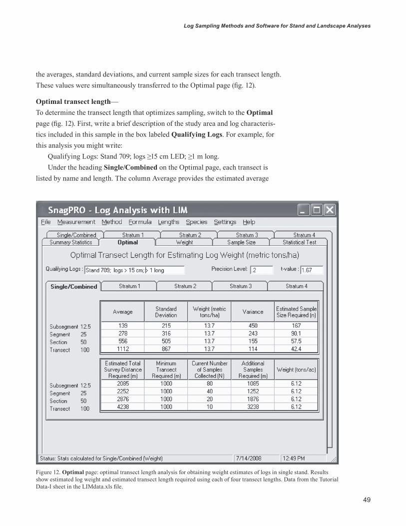
Log Sampling Methods and Software for Stand and Landscape Analyses
49
the averages, standard deviations, and current sample sizes for each transect length.
These values were simultaneously transferred to the Optimal page (fig. 12).
Optimal transect length—
To determine the transect length that optimizes sampling, switch to the Optimal
page (fig. 12). First, write a brief description of the study area and log characteris-
tics included in this sample in the box labeled Qualifying Logs. For example, for
this analysis you might write:
Qualifying Logs: Stand 709; logs ≥15 cm LED; ≥1 m long.
Under the heading Single/Combined on the Optimal page, each transect is
listed by name and length. The column Average provides the estimated average
Figure 12. Optimal page: optimal transect length analysis for obtaining weight estimates of logs in single stand. Results show estimated log weight and estimated transect length required using each of four transect lengths. Data from the Tutorial Data-I sheet in the LIMdata.xls file.

To select the optimal
transect length, look
at the Estimated
Total Survey
Distance Required
column. Which
transect section
requires the shortest
transect length?
GENERAL TECHNICAL REPORT PNW-GTR-746
50
values (squared intersects multiplied by specific gravity) from the Qualify column
for the four transect lengths. Standard deviations for these same values are shown
in the next column.
Under Weight (metric tons per hectare), the averages from the Qualify column
have been converted to actual weight measurements (fig. 12) using equation 5a.
Similarly, the standard deviations for each length are inserted into the equation to
obtain an estimate of the variance. For our example, SnagPRO estimates that the
stand supports about 15.2 metric tons/ha of logs in this size class. Notice that the
English equivalent is given in the last column of this section (about 6.8 tons/ac). The
column Estimated Sample Size Required calculates the total number of sampling
units (expressed in transect sections) required to obtain a weight estimate that is
within 20 percent of the true mean 90 percent of the time. In the Estimated Total
Survey Distance Required column, the sampling units required are expressed in
total length of transect.
To select the optimal transect length, look at the Estimated Total Survey
Distance Required column. Which transect section requires the shortest transect
length? In this example, the subsegments, which are 12.5-m long, require the least
amount (2012 m). By contrast, if 100-m transects are used, 4140 m of transect
length would be required.
We stated earlier that SnagPRO’s equations require a minimum of 60 samples.
The Minimum Transect Required column represents the minimum length in meters
of transect for a pilot sample. See the “Establishing Transects” section for more
detail. SnagPRO then evaluates the Current Number of Samples Collected and
calculates the Additional Samples Required. For this example, a little over 1000 m
of additional sampling (about 10 transects) would be required to obtain a weight
estimate within 20 percent of the true mean with a 90-percent confidence interval.
But are subsegments independent?
Test for independence—
To test for independence, switch to the Summary Statistics page and run the serial
correlation test. To do this:
1. Click on the Correlation button in the bottom-right corner of the screen.
2. Enter “Subsegment” when the first message box appears labeled
Correlation Length.
The message box displays the correlation coefficient (r = 0.083) and coefficient
of determination (r2 = 0.0069). The low r2 value (0.0069) implies that adjacent
subsegments along a transect are independent sampling units. Consequently, sub-
segments can be used for the remainder of the analysis along 100-m transects. One
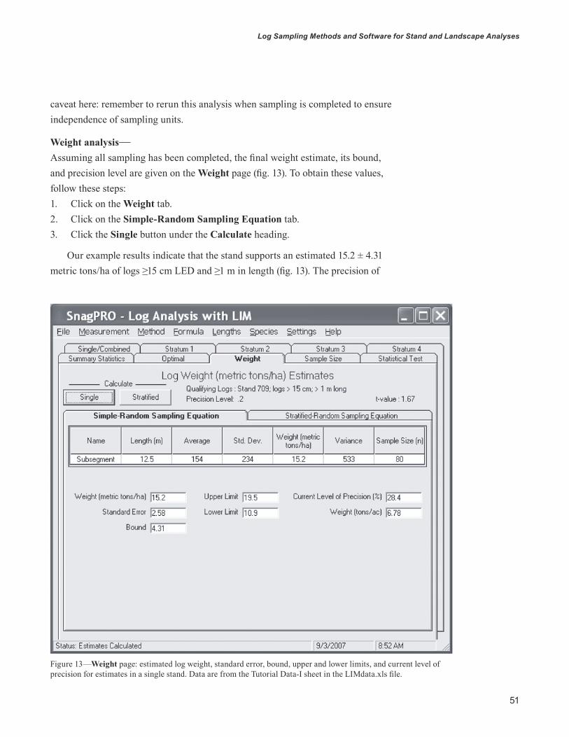
Figure 13—Weight page: estimated log weight, standard error, bound, upper and lower limits, and current level of precision for estimates in a single stand. Data are from the Tutorial Data-I sheet in the LIMdata.xls file.
Log Sampling Methods and Software for Stand and Landscape Analyses
51
caveat here: remember to rerun this analysis when sampling is completed to ensure
independence of sampling units.
Weight analysis
Assuming all sampling has been completed, the final weight estimate, its bound,
and precision level are given on the Weight page (fig. 13). To obtain these values,
follow these steps:
1. Click on the Weight tab.
2. Click on the Simple-RandomSamplingEquation tab.
3. Click the Single button under the Calculate heading.
Our example results indicate that the stand supports an estimated 15.2 ± 4.31
metric tons/ha of logs ≥15 cm LED and ≥1 m in length (fig. 13). The precision of

GENERAL TECHNICAL REPORT PNW-GTR-746
52
an estimate is calculated by dividing the bound by the mean. In this example, the
bound of 4.31 is divided by the mean of 15.2, and then multiplied by 100. The result
is 28.4 percent, which states that you are 90-percent confident that your density
estimate is within 28.4 percent of the true mean.
Density analysis by tally
The next step is to obtain density estimates using the tally data. To do this:
1. Click on Tally from the Formula menu. (Notice that the Formula list also
includes Density, but this calculation is performed only if log lengths have
been measured.)
2. Click Yes when asked “Do you want to clear this analysis and reload the
current database?”
3. Click the Set Criteria button.
4. Enter “Tally 1” when asked for the name of the column you would like
to tally.
5. Click on the tab at the top of the screen labeled Summary Statistics.
6. Click on the Single/Combined circle under the section labeled “Analyze
Data From.”
7. Complete the process by clicking on the Calculate Statistics button.
Switch to the Optimal page to determine which transect length is best for
density estimates. Example results estimate that the stands contain 248 logs/ha (100
logs/ac). Looking under the Estimated Total Survey Distance Required column,
we see that subsegments again appear to be the optimal transect length within this
stand. They require only 1242 m of transect. Therefore, only two or three more
transects are needed to reach the desired precision. But are subsegments indepen-
dent for density estimates? To test for independence:
1. Switch back to the Summary Statistics page.
2. Click on the Correlation button.
3. Enter “Subsegment” into Correlation Length box.
The message box displays the correlation coefficient (r = 0.115) and the coeffi-
cient of determination (r2 = 0.013) for log densities. Similar to the weight correlation
analysis, subsegments appear to be independent.
To obtain the current level of precision of your density estimate:
1. Click on the Tally page tab.
2. Highlight the Simple-RandomSamplingEquation tab.
3. Click the Single button.
4. Enter “24” into the Single Stratum box.

Log Sampling Methods and Software for Stand and Landscape Analyses
53
It is estimated that there are 248 ± 53.8 logs/ha in this stand. Precision is just
below 22 percent.
Conclusionsforsingle-standweightanddensityanalysis
From the pilot survey data alone, the desired precision for density has nearly been
reached. To obtain this precision for weight, however, about 10 additional tran-
sects would have to be sampled. If, however, the current precision of 28 percent is
deemed adequate, sampling can cease. If it is deemed important to improve preci-
sion to ≤20 percent, then the 10 additional transects should be surveyed.
Example II: English Parameter Estimates and Statistical Test for a Stratified Landscape Using SPM
Background information
A second example is forest compliance monitoring for wildlife, specifically to
evaluate whether log management goals have been met on a landscape scale.
The landscape comprises mixed-conifer forest communities. Many areas have
been clearcut or seed-tree harvested. The remaining stands are mature or old-
growth forests.
Current wildlife guidelines stipulate retention of an average of 20 logs/ac and
>2 percent log cover across the landscape (composed of logs with a LED >10 in and
>6 ft long). The monitoring goal is to estimate both density and percentage cover
within 20 percent of the true mean 90 percent of the time to evaluate guidelines.
Woodpecker and small mammal use of logs also is of interest within the different
forest structural conditions.
Stratification—
Aerial photographs show that the landscape is highly fragmented and geospatial
data verify that clearcut and seed-tree harvests have been the primary methods
of timber harvesting. Therefore, stands will be placed into one of two strata: (1)
harvested or (2) unharvested mature/old-growth stands. A map of the stand poly-
gons for each stratum is established with GIS. Each stand’s acreage and the total
acreage within each stratum is summed. There are 750 and 224 ac in strata 1 and
2, respectively. Field reconnaissance is then done to verify that each stand has been
placed in the proper stratum.
Pilot survey—
An initial reconnaissance indicates that it is uncommon to intersect >10 large
logs (>10 in LED and >6 ft long) per 330 ft of transect (see table 2 for details).
Furthermore, sampling must be as efficient as possible because of substantial travel

GENERAL TECHNICAL REPORT PNW-GTR-746
54
required to sample at random points across the landscape. Consequently, SPM is
selected as the sampling method. Also, LED data are collected as a continuous
variable so that analysis can be done on a variety of size classes.
Five stands in each stratum are randomly selected in which two 400-ft-long
transects are established (fig. 6). Starting points for each transect are selected by
randomly placing a grid over each stand and randomly choosing a grid intersection
for the starting point. The compass direction is also random.
Each transect is assigned a number, and then divided into eight 50-ft subseg-
ments, numbering them 1 through 8 so that during analysis, the shorter subseg-
ments can be joined into 100-ft (segments) and 200-ft (sections) transect lengths.
Then SnagPRO can help determine the best transect length for each stratum. The
bounce-back method is used for transects heading outside stand boundaries (fig. 7).
Continue to sample with standardized transect lengths and include stand edges.
The SPM Field Form sheet found in the file named SPMdata.xls (fig. 9) is used
as the field form. (See “Field Forms” under “General Surveying Procedures” for
complete details.) Appendix 3 is customized to describe the information required
under each field heading, as an aid to field sampling, and copies of figures 4 and 5
also are made to help guide fieldwork.
Only the portions of logs >10 in LED and >6 ft long within sampling boundar-
ies are measured. The LEDs of each log are measured as shown in fig. 5. For each
log, record:
1. Diameter (in) of large end regardless if it is in or out of the plot.
2. Whether the endpoint of the log (fig. 5) is in (enter 1) or out (enter 0) of
the plot.
3. Diameter (in) of largest portion of the log contained within the plot.
4. Diameter (in) of smallest portion of the log contained within the plot.
5. Length (ft) of portion of log contained within the plot.
6. Condition based on three-class decay system (Bull and others 1997).
7. Species.
8. Wildlife use: 0 = no use, 1 = woodpecker foraging, 2 = small mammal
middens.
For subsegments where no qualifying logs are encountered, enter “9999” in the
LED column.
Data entry—
To enter your own data, use Sheet 1 of the file SPMdata.xls. In our example, data
have been entered in Excel as part of the tutorial. Open the file SPMdata.xls and

Log Sampling Methods and Software for Stand and Landscape Analyses
55
click on the tab in the lower left corner that is labeled “Tutorial Data-II.” Here
you will find that the log data collected from 20 transects have been entered for
our example.
Consecutive subsegments—
Before analysis, sort transects and subsegments in ascending order to ensure that
there are eight subsegments for each transect. In Excel, click a single cell in the
first row and then click Data | Sort. Make sure that the entire data set has been
highlighted for sorting. Then select Sort By transect and Then By subsegment.
Scroll through the entire data set to ensure that eight subsegment lengths have
been entered for each transect and the beginning subsegment of each transect is
numbered “1.”
CreatingaCSVfile—
SnagPRO imports only CSV files. To create a CSV file, follow these steps:
1. Activate the Tutorial_Data_II sheet by clicking anywhere on the sheet.
2. Select File | Save As.
3. Click Save as Type at the bottom of the Save As message box.
4. Select “CSV (comma delimited)(*.csv)”.
5. Assign a new file name in the file name box.
6. Click Save. When saving as a CSV file, only the active sheet is retained.
By saving the file with a different name, the original file is kept intact.
7. Click OK and Yes for first and second warning boxes, respectively.
Importing to SnagPRO—
Import the CSV file of log data using these steps:
1. Launch SnagPRO by double-clicking on the desktop icon or the executable
file—SnagPRO.exe.
2. Click Logs.
3. Go to Measurement, and click English.
4. Go to Method and click SPM.
5. Go to File | Open. In the message box “Look In,” browse to the folder
containing the CSV data and select the file name.
This should successfully import the CSV file onto the Single/Combined page of
SnagPRO. Note that the Section and Segment columns have been added to your file.
SnagPRO combined consecutive subsegments (50-ft lengths) into segments (100-ft
lengths), and segments into sections (200-ft lengths) to allow for optimal transect
length analysis.

GENERAL TECHNICAL REPORT PNW-GTR-746
56
Formula entry—
The next step is to have SnagPRO insert the appropriate formula into the Qualify
column for each stratum. This formula determines which logs are included in the
analysis. To do this:
1. Click on the Stratum 1 tab to activate the sheet.
2. Click on Density under the Formula menu.
3. Click the Apply and Sort button.
To create the correct formula for all logs >10 in LED, enter
1. “10” for LED.
2. “0” for EstimLength because all logs will be included.
3. “3” for Condition (all decay classes are included).
4. “9999” for Species (all log species included).
SnagPRO evaluates each log for the criteria listed above. For logs meeting all
criteria, and with endpoints contained within the plot, SnagPRO places a “1” in the
Qualify column. Note that log lengths are based on the EstimLength column rather
than the Length column. The Length column only represents the length of the logs
within the strip plots and not their entire lengths. EstimLength is the total length of
log, both inside and outside the plot. See EstimLength in the “SnagPRO’s Equa-
tions” section for more information.
Analyzing by transect length—
SnagPRO now calculates averages and standard deviations for each transect length
within each stratum on the Summary Statistics page. To calculate the statistics for
stratum 1:
1. Click on the Summary Statistics tab.
2. Click on the Stratum 1 circle in the Analyze Data From section.
3. Click on the Calculate Statistics button.
To determine the transect length that optimizes sampling in stratum 1, switch
to the Stratum 1 sheet on the Optimal page. First, write a brief description of the
study area and log characteristics included in this sample in the box labeled “Quali-
fying Logs.” For example, for this analysis you might write:
Qualifying Logs: Stratum 1; >10 cm LED; >1 m long.
To the far left on this page, each transect is listed by name and length. The
Average column provides the estimated average values (summed endpoints) from
the Qualify column for the four transect lengths. Standard deviations for these
same values are shown in the next column. Under Density (logs/ac), the summed
endpoints from the Qualify column have been converted to density.

Log Sampling Methods and Software for Stand and Landscape Analyses
57
SnagPRO estimates that there are 14.5 logs/ac. Notice that the metric equiva-
lent is given in the last column (35.9 logs/ha). The column Estimated Sample Size
Required calculates the total number of sampling units (expressed in number of
strip plots) required to obtain a density estimate within 20 percent of the true mean
90 percent of the time. In the Estimated Total Survey Distance Required column,
the sampling units required are expressed in total length of transect.
To select the optimal transect length, look at the Estimated Total Survey
Distance Required column. Which transect section requires the shortest transect
length? In this stratum, the segments, which are 100 ft long, require the least
amount (21,905 ft). Notice that the 200-ft lengths (section) are the second-best
choice, with 22,226 ft of transect required.
Earlier, we stated that SnagPRO’s equations require a minimum of 60 samples.
The Minimum Transect Required column represents the minimum length in feet of
transect for a pilot sample. See the “Establishing Transects” section for more detail.
SnagPRO then evaluates the Current Number of Samples Collected and calculates
the Additional Samples Required.
For this stratum, about five times as many segments as have been sampled
are needed to obtain a density estimate with desired precision. Sampling effort is
high because of low log density and high variance within this stratum. In addition,
SnagPRO currently considers this a single landscape, which is necessary to deter-
mine the optimal transect length. Sampling effort will be less within this stratum,
however, once it is considered in conjunction with stratum 2.
Now check and see if segments can be considered independent sampling units.
To do this:
1. Switch back to the Summarize Statistics page.
2. Click on the Correlation button.
3. Enter “Segment” into the Correlation box.
The message box displays the correlation coefficient (r = 0.105) and the coef-
ficient of determination (r2 = 0.011) for log densities in stratum 1. Based on these
results, adjacent segments can be considered independent and used as the sampling
unit for stratum 1.
To determine the optimal transect length for stratum 2, repeat all steps de-
scribed for stratum 1. The stratum 2 sheet on the Optimal page shows that the
estimated log density for stratum 2 (mature/old-growth stands) is 39.9 logs/ac and
transect lengths (400-ft lengths) appear to optimize the sampling effort (7,754 total
ft of transect required).

Figure 14—Densities page: estimated log density, standard error, bound, upper and lower limits, and current level of precision for estimates in on a stratified landscape. Data are from the Tutorial Data-II sheet in the SPMdata.xls file.
GENERAL TECHNICAL REPORT PNW-GTR-746
58
Stratifieddensityanalysis—
To obtain an estimate of the required sample size for the entire landscape, we first
need an estimate of the stratified mean density to enter in the sample size equation.
To do this:
1. Go to the Densities page (fig. 14).
2. Click on the StratifiedRandomSamplingEquation tab.
3. Enter “750” into the Stratum 1 box in the Stratum Size (acres) section.
4. Enter “224” into the Stratum 2 box.
5. Click the Stratified button under Calculate.
Once the Stratum Sizes (acres) have been filled in, SnagPRO transfers all statis-
tics from the Optimal page to the Density page. The results on the Density page (fig.
14), estimate an average density of 20.3 ± 5.81 logs/ac. Precision is 28.6 percent.

Figure 15—Sample size page. Optimal and proportional sample size calculations for obtaining estimates of log density on a landscape containing two strata. Data are from the Tutorial Data-II sheet in the SPMdata.xls file.
Log Sampling Methods and Software for Stand and Landscape Analyses
59
Sample size determination—
The next step is to determine the required sample size to obtain the desired
precision. Sample sizes for stratified subwatersheds are calculated on the Sample
Size page, so activate this page (fig. 15). Notice that SnagPRO transferred the
statistics to the Sample Size page once the stratified density estimate on the Density
page was calculated.
At the bottom of the Sample Size page (fig. 15), output from two sample
size equations are shown—Optimal Allocation and Proportional Allocation.
The optimal allocation method, which incorporates the stratum variance in its

GENERAL TECHNICAL REPORT PNW-GTR-746
60
calculations, estimates that 93 samples are required to obtain a stratified mean
within 20 percent of the true mean, 90 percent of the time. These 93 samples are
then divided between the two strata: 75 samples in stratum 1 (harvested stands) and
19 samples in stratum 2 (mature/old-growth stands). Segments are the sampling unit
for stratum 1 and transects are the sampling unit for stratum 2. These estimates are
equal to about 7,500 ft of transect in stratum 1 and 7,600 ft in stratum 2. Recall,
however, that 4,000 ft of transect have already been sampled in both strata.
On the bottom right of the page is the heading “Proportional Allocation.” This
method uses the overall variance of the subwatershed and then allocates the samples
based on the size of each stratum. Results show that 103 samples are needed to
obtain the desired precision, which in turn requires 8,000 ft of transect in stratum
1 and 9,600 ft in stratum 2.
Both sample size equations agree that additional samples are needed. It is
important to remember that sample size requirements may change with additional
sampling, owing to changes in the variance of estimates. This possibility increases
if the pilot sample is ultimately shown to be a poor representation of the varia-
tion within a stratum. Consequently, the best way to avoid oversampling (where
large sample sizes are required) is to periodically enter your data, and re-run the
SnagPRO analysis. In addition, sometimes it is helpful to “override” the default for
transect length. For example, what would happen if you changed the transect length
to something shorter in stratum 2, such as segments? To do this, follow these steps:
1. From the Settings menu, highlight Optimal Selection.
2. Click on Stratum 2.
3. Check Segment instead of Auto.
By overriding the default transect length for stratum 2, precision changes
slightly, from 28.6 to 29.2 percent. Sample size requirements, however, drop from
7,600 ft to only 4,800 ft under the optimal allocation method. However, sample
requirements in stratum 1 increase to 8,700 ft. These changes demonstrate the
sensitivity of the equations and the chosen sample size. Given the uncertainty, it
may be best to sample about five additional stands within each stratum, and then
reanalyze the data to see how the additional information affects the chosen transect
length and precision.
Compare to target density—
Once 60 samples have been collected, the test of whether the estimated density
of qualifying logs meets the targeted density of 20 logs/ac can be done. The
null hypothesis is that no difference exists between the estimated and targeted
log densities.
Both sample size
equations agree
that additional
samples are needed.
It is important
to remember
that sample size
requirements
may change with
additional sampling,
owing to changes
in the variance
of estimates.

Figure 16—Statistical test page. Graph depicting test for significant differences between estimated and targeted densities of qualifying logs on stratified landscape. Estimated value and its bound are from the Densities page (fig. 14). Data are from the Tutorial Data-II sheet in the SPMdata.xls file.
Log Sampling Methods and Software for Stand and Landscape Analyses
61
Go to Statistical Test page to conduct the test (fig. 16).
Follow these steps:
1. Enter the targeted density of “20” into the box labeled Target Value.
2. Enter the estimated log density of “20.3 logs/ac” into the box labeled
Estimated Value.
3. Enter “5.81” into the estimated Bound box.
Results are automatically plotted as a graph (fig. 16), which shows that the line
representing the target density is within the upper and lower limits of the estimated
density, just below the targeted density. Consequently, the null hypothesis is not
rejected. That is, results indicate, with 90 percent confidence, that the log density
on this landscape is adequate to meet agency guidelines.

GENERAL TECHNICAL REPORT PNW-GTR-746
62
Percentage cover analysis—
To analyze percentage cover estimates, change the variable selection:
1. Click on Percent Cover under the Formula menu.
2. Click Yes when asked “Do you want to clear this analysis and reload the
current data set?”
At this point, the steps to conduct the analysis for percentage cover are identical
to the steps taken for the density analysis:
1. Activate the Stratum 1 page.
2. Click the Set Criteria button.
3. Enter the correct log characteristics for LED, EstimLength, Condition
and Species.
4. Switch to the Summary Statistics page.
5. Click on the Stratum 1 circle.
6. Click the Calculate Statistics button.
7. Click on the Stratum 2 circle.
8. Click the Calculate Statistics button.
9. Switch to the Optimal page to view results for stratum 1.
Percentage cover for stratum 1 is estimated to be 0.54 percent. Based on these
results, it appears that segment lengths are the optimal transect length requiring
11,872 ft of transect. The serial correlation test conducted on the Summary Statis-
tics page (see instructions above from density analysis) indicates that segments are
independent sampling units (r2 = 0.0008).
Clicking on the Stratum 2 sheet of the Optimal page shows an estimated cover
value of 2.6 percent for stratum 2. In this stratum, the subsegments, or shortest
transects, are the optimal length. Only 3,666 ft of total transect is required (which
has already been collected) to obtain an estimate that is within 20 percent of the
true mean, 90 percent of the time. Serial correlation test conducted on the Sum-
mary Statistic page also shows subsegments to be independent (r2 = 0.0008).
To conduct the statistical test to compare cover estimates, first obtain a strati-
fied estimate for cover:
1. Activate the Percent Cover page.
2. Click on the Stratified-RandomSamplingEquation sheet.
3. Enter “750” into the Stratum 1 area box.
4. Enter “224” into the Stratum 2 box.
5. Click the Stratified button.

Figure 17—Statistical test page. Graph depicting test for significant differences between estimated and targeted percent cover values of qualifying logs on stratified landscape. Estimated value and its bound are from the Percent Cover page. Data are from the Tutorial Data-II sheet in the SPMdata.xls file.
Log Sampling Methods and Software for Stand and Landscape Analyses
63
Results indicate a stratified estimate of percentage cover of 1.02 ± 0.184. The
current precision (18 percent) exceeds the goal of being within 20 percent of the
true mean. To test for a difference between targeted and estimated percentage
cover, switch to the Statistical Test page.
Of interest is whether the estimated cover of logs across this landscape equals
or exceeds the targeted value of 2 percent. In this case, the null hypothesis is that
no difference exists between estimated cover of logs across this landscape and the
target of 2 percent. To test, enter the percentage cover estimate, its bound, and the
target value into the appropriate boxes on the Statistical Test page (fig. 17).

GENERAL TECHNICAL REPORT PNW-GTR-746
64
The resulting graph shows that the red line (top line), representing the target
cover, is not within the upper and lower limits of cover estimated for the entire
landscape (fig. 17). This is in contrast to the results observed from the density
analysis. Therefore, the null hypothesis of “no difference between the harvested
and unharvested density estimates,” is rejected. Results suggest that you can be
90-percent confident that log cover across the landscape does not equal or exceed
the target of 2 percent.
Wildlife use—
The final objective is to evaluate wildlife use of logs in harvested stands versus
unharvested stands. To calculate use of logs with signs of woodpecker foraging:
1. Activate the Summary Statistics page.
2. Click on the Stratum 1 circle from the Analyze Data From section.
3. Click on the Wildlife Use button.
4. Enter “10” into the message box labeled LED.
5. Enter “0” into the EstimLength box.
6. Enter “3” into the Condition box.
7. Enter “9999” into the Species box.
8. Enter “1” into the Wildlife use box.
Results in the Wildlife section of this page show that within Stratum 1, there
were 38 logs available for woodpecker foraging use and 6 showed signs of use for a
use of 15.8 percent in harvested stands. For stratum 2, results show that out of 126
logs available, 21 showed woodpecker foraging signs for a use of 16.7 percent in
unharvested stands.
For small mammal use (wildlife code = 2) in stratum 1, 38 logs were available
and 3 had evidence of middens, resulting in use of 7.9 percent in harvested stands.
This compares to 40 out of 126 available logs having small mammal middens, for a
use of 31.7 percent in unharvested stands.
Conclusions for multiple strata using SPM—
Statistical tests comparing log estimates with management goals revealed different
results. Although log densities met agency guidelines, the percentage of cover did
not. These results suggest that an adequate number of logs were retained in harvest-
ed stands, but were short in length or small in diameter. Consequently, the small
size or short length of logs contributed little toward cover. Results of the wildlife
use analysis suggest that woodpecker foraging use was about equal in harvested
and unharvested stands. By contrast, squirrel use of logs in unharvested stands was
about four times that in harvested stands.
These results
suggest that an
adequate number of
logs were retained
in harvested
stands, but were
short in length or
small in diameter.
Consequently, the
small size or short
length of logs
contributed little
toward cover.

Log Sampling Methods and Software for Stand and Landscape Analyses
65
Example III: Metric Parameter Estimates for a Stratified Landscape Using a Combination of LIM and SPM
Background information—
In this example, two resource disciplines are interested in information on log condi-
tions in a subwatershed. Fire managers are interested in volume of logs ≥15 cm
LED and ≥1 m long for separate areas within the subwatershed. Wildlife managers
need a stratified estimate of log volume for the entire subwatershed, but only for
larger logs (≥25 cm LED and ≥1 m long). Both fire and wildlife managers want
estimates to be as precise as possible because of pending management actions, but
budget constraints may limit the number of stands that can be sampled.
Aerial photographs and geospatial data indicate that less than half the subwa-
tershed has been harvested in the past 40 years. Log volumes are anticipated to be
low in these stands. About one-third of the subwatershed is composed of mature
forests with pockets of old-growth interspersed. Of special concern, however, are
a number of stands that have undergone high mortality owing to an outbreak of
spruce budworm (Choristoneura occidentalis Free.) (Sheehan 1996) during the past
10 years. Travel is difficult within these stands because of the high log abundance.
Stratification—
Based on a ground reconnaissance, the harvested stands appear to be accurately
represented in the GIS database and support a low number of logs. Log density is
initially checked by estimating how many logs are intersected by several randomly
established transect lines within the typical harvested stand on this subwatershed
(see table 2 for details). On average, it appears that three to four logs are intersected
with every 100 m of transect in the harvested stands.
The remaining unharvested stands have greater log abundance, and individual
stands require visual examination to determine whether abundance is moderate
or high. Reconnaissance indicates high log abundance in stands that are undergo-
ing the budworm outbreak; in these stands, over 30 logs per 100-m transect were
intersected. The remaining stands appear to support moderate abundance, with
an average of 10 to 15 logs per 100 m of transect. Based on this information, three
strata are established: (1) recent clearcut and seed-tree harvest units with low log
abundance, (2) mature stands with moderate log abundance, and (3) mature stands
with high log abundance. For this example there are 812, 654, and 490 ha in strata
1, 2, and 3, respectively.
In strata 2 and 3 where log abundance is moderate and high, respectively, LIM
(table 2) is used to sample logs. Because of the low abundance of logs in harvested
stands, however, SPM is used for estimates of log volume in stratum 1 to minimize
the number of transects required.
GENERAL TECHNICAL REPORT PNW-GTR-746
66
Pilot survey—
Five stands from each stratum are randomly selected for sampling. Starting points
for each transect are selected by placing a grid over each stand and randomly
choosing a grid intersection for the starting point. The compass direction also is
randomly determined.
Each 100-m transect is divided into eight 12.5-m-long subsegments. Each
transect is assigned a unique numeric identifier while numbering the subsegments 1
through 8. This is done so that the shorter subsegments can be evaluated as 25- and
50-m transect sections to determine the optimal transect length during analysis.
The bounce-back method is used to keep the transect within the sampling area that
otherwise would extend beyond stand boundaries, while continuing to sample with
standardized transect lengths to include stand edges (fig. 7).
The SPM Field Form sheet, found in the file named SPMdata.xls (fig. 9), is
used as the field form in stratum 1. (See “Field Forms” under “General Surveying
Procedures” for complete details.) Appendix 3 is customized to describe the infor-
mation required under each field heading as an aid to field sampling, and copies of
figures 4 and 5 also are made to help guide fieldcrews to determine the appropriate
place to measure LED.
Only the portions of logs ≥15 cm LED and ≥1 m length within the boundaries
are measured. The LEDs of each log are measured as shown in figure 5. For each
qualifying log, record:
1. Size class (record either 15 for≥15 or 25 for≥25) of LED.
2. Diameter (cm) of largest portion of the log contained within the plot.
3. Diameter (cm) of smallest portion of the log contained within the plot.
4. Length (m) of portion of log contained within the plot.
For subsegments where no qualifying logs are encountered, “9999” is entered
in the LED column. For data collection in strata 2 and 3, make copies of the data
entry sheet found in the file named LIMdata.xls (fig. 8) for use as a field form. (See
“Field Forms” under “General Surveying Procedures” for complete details.) Cus-
tomize appendix 2 to describe the information required under each field heading of
the field form, as an aid to fieldwork.
In the field, for each qualifying log intersected, the following volume measure-
ments are recorded:
1. Diameter (cm) at intersection.
2. Size class (either 15 or 25 cm) of LED.
For subsegments where no qualifying logs are intersected, “9999” is entered in
the LED column.

Log Sampling Methods and Software for Stand and Landscape Analyses
67
Data entry—
When using a combination of LIM and SPM, data from each stratum must be stored
separately because of differences in data collection techniques and equations. First,
obtain an estimate of the variable of interest (in this case, volume) for each stratum.
Then estimates from each stratum can be entered in a special page in SnagPRO
named Combination found under the Method menu. Estimates of the stratified
mean, precision level, and sample sizes within each stratum and across the land-
scape are then calculated on this page.
To enter LIM data analysis, use Sheet 1 of the file LIMdata.xls. For SPM
analysis, use Sheet 1 of the SPMdata.xls file. For this example, however, the data
have already been entered. For LIM analysis, open the file LIMdata.xls and click
on the tab in the lower left corner that is labeled “Tutorial Data-III-Stratum 2.”
Here you will find log data collected from 10 transects for this stratum.
Consecutive subsegments—
Before analyses, sort transects and subsegments in ascending order to ensure that
there are eight subsegments for each transect. In Excel, click a single cell in the
first row and then click Data | Sort. Make sure that the entire data set has been
highlighted for sorting. Then select Sort By transect and Then By subsegment.
Scroll through the entire data set to ensure that eight subsegment lengths have
been entered for each transect, and the beginning subsegment of each transect is
numbered “1.”
CreatingaCSVfile—
SnagPRO imports only CSV files. To create a CSV file for stratum 2, follow
these steps:
1. Activate the “Tutorial_Data_III-Stratum 2” sheet by clicking anywhere on
the sheet.
2. Select File | Save As.
3. Click Save as Type at the bottom of the Save As message box.
4. Select “CSV (comma delimited)(*.csv).”
5. Assign a new file name in the file name box.
6. Click Save. When saving as a CSV file, only the active sheet is retained.
By saving the file with a different name, the original file is kept intact.
7. Click OK and Yes for first and second warning boxes, respectively.
To create the CSV file for stratum 3, repeat the procedure above with the
worksheet labeled “Tutorial_Data_III-Stratum 3” found in the LIMdata.xls file. To
create the CSV file for stratum 1, repeat the procedure above using the worksheet
labeled “Tutorial Data-III” found in the SPMdata.xls file.
GENERAL TECHNICAL REPORT PNW-GTR-746
68
Importing to SnagPRO—
Import the CSV file of stratum 2 log data using these steps:
1. Launch SnagPRO by double-clicking on the desktop icon or the executable
file—SnagPRO.exe.
2. Click Logs.
3. Go to Measurement and click Metric.
4. Go to Method and click LIM.
5. Go to File | Open. In the message box “Look In,” browse to the folder
containing the CSV data, and select the file name.
This should successfully import the CSV file onto the Single/Combined page
of SnagPRO. Although there are three strata for this analysis, each is treated as if
it is part of a nonstratified landscape to obtain the information necessary for input
onto the Combination page. Therefore, all analyses will be based on the Single/
Combined page.
Note that additional columns have been added to your file. The Section and
Segment columns were inserted between Transect and Subsegment. SnagPRO com-
bined consecutive subsegments (12.5-m lengths) into segments (25-m lengths), and
segments into sections (50-m lengths) to allow for optimal transect length analysis.
Formula entry—
The next step is to have SnagPRO insert the appropriate formula in the Qualify
column. This formula determines which logs are included in the current analysis.
Begin with all logs >15 cm LED. To do this, click on Volume under the Formula
menu on the Single/Combined page. Then click on Set Criteria button located in
the bottom-left of the screen.
To create the correct formula, based on your survey objectives, enter:
1. “15” for LED.
2. “0” for Length (the default when log lengths are not measured).
3. “0” for Condition (the default when log condition is not measured).
4. “9999” for Species (all log species are considered).
SnagPRO evaluates each log by the criteria listed above. For logs meeting all
criteria, SnagPRO takes the intersect diameter of each log, squares it, and places
this value in the Qualify column. Then SnagPRO inserts these values in the LIM
estimator (equation 4a) to obtain volume estimates.
Analyzing by Transect Length—
SnagPRO calculates averages and standard deviations for each transect length
within each stratum on the Summary Statistics page. To calculate the statistics for
the current forest conditions:

Log Sampling Methods and Software for Stand and Landscape Analyses
69
1. Click on the Summary Statistics tab.
2. Click on the Single/Combined circle in the Analyze Data From section.
3. Click on the Calculate Statistics button.
SnagPRO subtotals the values for each transect length (Subsegment_12.5,
Segment_25, Section_50, and Transect_100). The number on the end of each label
gives the length of the transect in meters. To the right of the subtotaled values are
the averages, standard deviations, and current sample sizes for each transect length.
These values were simultaneously transferred to the Optimal page.
Optimal transect length—
To determine the transect length that optimizes sampling in current forest condi-
tions, switch to the Optimal page. First, write a brief description of the study area
and log characteristics in the box labeled Qualifying Logs. For example, for this
analysis you might write:
Qualifying Logs: Stratum 2; logs ≥15 cm LED; ≥1 m long.
Under the heading Single/Combined on the Optimal page, notice each tran-
sect listed by name and length. The Average column provides the estimated average
values (squared intersects multiplied by specific gravity) from the Qualify column
for the four transect lengths. Standard deviations for these same values are shown
in the next column.
Results under the heading Volume (m3/ha) show that this stand supports about
72.8 m3/ha of logs in this size class of interest (≥15 cm LED; ≥1 m long). Note that
the English equivalent is given in the last column (1,041 ft3/ac). The two columns
labeled Estimated Sample Size Required and Estimated Total Survey Distance Re-
quired, calculate the total number of transect sections and total length of transect,
respectively, required to obtain a weight estimate within 20 percent of the true
mean 90 percent of the time.
To select the optimal transect length, look at the column Estimated Total Sur-
vey Distance Required. In this example, the subsegments, which are 12.5 m long,
require the shortest length for sampling (2304 m). By contrast, if 100-m transects
are used, 6942 m of transect length would be required. But are subsegments inde-
pendent? To test for independence:
1. Switch back to the Summary Statistics page.
2. Click on the Correlation button.
3. Enter “Subsegment” into Correlation Length box.
The message box displays the correlation coefficient (r = 0.255) and the coef-
ficient of determination (r2 = 0.067). Based on these results, subsegments appear
independent and may be used in this analysis.

GENERAL TECHNICAL REPORT PNW-GTR-746
70
The last column in section two of the Optimal page is Additional Samples Re-
quired. This states how many meters of transect are still required to obtain a precise
estimate after taking into account the sampling completed during the pilot survey.
For this example, a little over 1300 m additional sampling would be required in
stratum 2 to obtain a volume estimate within desired precision.
Volume analysis—
Volume estimates with a bound and precision level are given on the Volume page in
SnagPRO. To obtain these values:
1. Click on the Volume tab.
2. Click on the Simple-RandomSamplingEquation tab.
3. Click the Single button under the Calculate heading.
Results indicate that this stand supports an estimated 72.8 ± 22.1 m3/ha of logs
in this size class. (Recall that the precision of an estimate is calculated by dividing
the bound by the mean.) In this example, the estimated precision is 30.4 percent,
which can be interpreted as being 90 percent confident that the volume estimate in
stratum 2 is within 30.4 percent of the true volume. At this point, a decision must be
made as to whether the estimate is precise enough to meet management objectives,
or whether to sample along 13 more 100-m transects (as indicated on the Optimal
page) to improve the precision within this stratum.
To ensure that accurate numbers are entered onto the Combination page, print
the results from the Volume page. To do this:
1. From the File menu select Print Preview.
2. Then choose either Print Portrait or Print Landscape.
3. Click Print.
The next step is to obtain volume estimates of logs ≥25 cm LED. To do this,
repeat all steps listed above, starting with the “Formula Entry” section, but when
prompted to enter the qualifying LED, enter 25 instead of 15.
On the Optimal page, results indicate that subsegments are the optimal transect
length, requiring about 3354 m of transect. Check if these lengths are independent
by clicking on the Correlation button on the Summary Statistics page. Results
show that adjacent subsegments for this log size class are independent (r = 0.17; r2 =
0.029). Therefore, we will proceed with this length.
On the Volume page, click on the Single button to have the results from the
Optimal page transferred. It is estimated that there are 54.1 ± 19.8 m3/ha of logs
in this size class (773 ft3/ac). Precision is 36.6 percent. Print this page to save the
statistics for input onto the Combination page.

Log Sampling Methods and Software for Stand and Landscape Analyses
71
Stratum 3 analysis—
To obtain volume estimates for stratum 3, import the data by clicking on File and
directing SnagPRO to the CSV file containing data for stratum 3. Then repeat
all instructions for stratum 3, as listed above for stratum 2. Print results from the
Volume page for both log size classes when completed.
Based on the results shown on the Optimal page, stratum 3 supports an estimat-
ed 145 m3/ha of logs ≥ 15 cm LED, or 2,076 ft3/ac. It appears that the best transect
length in stratum 3 is the segment. Using this length requires an estimated 443 m of
transect, assuming the segments are independent.
The serial correlation test, however, shows that segments may not be indepen-
dent (r = 0.45). Values above this level are not considered independent (r = 0.403;
r2 = 0.163). Although we will continue to use this transect length for our analysis,
assume for a moment that we want to choose a different length. The next best
choice would be subsegments based on the results on the Optimal page. The cor-
relation test on subsegments shows that this length can be considered independent
(r = 0.063; r2 = 0.004). Subsegments, rather than segments, are better sampling units
in this case because of the systematic distribution of logs. Segments were likely
regularly hitting, or missing, clumps of logs, whereas using subsegments minimized
this phenomenon. Note that the optimal transect length identified by SnagPro can
be overriden by selecting a different Optimal Selection from the Settings menu
and using the resulting statistics in the analysis.
The Volume page shows that stratum 3 supports an estimated 145 ± 19.3 m3/ha.
In addition, because log volume was consistently high throughout the stands, with
low variability, the precision for this size class, 13.3 percent, has exceeded the
desired level. Print the results on the Volume page for use on the Combination page.
Repeating this process for large (≥ 25 cm LED) logs in stratum 3 shows a vol-
ume of 89.1 ± 20.6 m3/ha. The precision of 23.1 percent is approaching the desired
level of 20 percent. Subsegments provide the most precise measurement and can
be considered independent (r = 0.187; r2 = 0.035). Sample size required equals 1334
m of transect length. Print results on the Volume page for use on the Combination
page. This completes the analysis with LIM data.
Strip-plotmethodofanalysis—
To obtain SPM volume estimates for stratum 1, import the data into the SPM
portion of SnagPRO by using the following steps:
1. Click Logs under Habitat Component.
2. From the Method menu click SPM.
3. Click Yes to reaffirm a new analysis.
Subsegments, rather
than segments, are
better sampling units
in this case because
of the systematic
distribution of logs.
Segments were likely
regularly hitting,
or missing, clumps
of logs, whereas
using subsegments
minimized this
phenomenon.

GENERAL TECHNICAL REPORT PNW-GTR-746
72
4. Click Open in the File menu.
5. Direct SnagPRO to the folder where the CSV file containing the SPM data
can be found.
This should successfully import the CSV file onto the Single/Combined page
of SnagPRO. Note that the Section and Segment columns have been added to the
file, inserted between Transect and Subsegment. Also note that although informa-
tion about endpoints (for density estimates) were not collected, a column labeled
Endpoint appears on the data sheet. This formatting is necessary for SnagPRO to
work properly.
Formula entry—
The next step is to have SnagPRO insert the appropriate formula in the Qualify
column for stratum 1. This formula determines which logs are included in the cur-
rent analysis. To do this:
1. From the Formula menu, select Volume.
2. “10” for LED.
3. “0” for EstimLength because you want all logs to be included and only
logs ≥1 m long were measured.
4. “3” for Condition (all decay classes considered).
5. “9999” for Species (all log species considered).
For logs meeting the above criteria, SnagPRO calculates the volume of
each portion of the log contained within the plot. This value is placed in the
Qualify column.
Analyzing by transect length—
SnagPRO calculates averages and standard deviations for each transect length
within each stratum on the Summary Statistics page. To calculate the statistics for
stratum 1:
1. Click on the Summary Statistics page.
2. Click on the Single/Combined circle in the Analyze Data From section.
3. Click on the Calculate Statistics button.
Optimal transect length—
Switch to the Optimal page and write a brief description of the stratum and size
class of log being analyzed. For example:
Qualifying Logs: Stratum 1; SPM; logs ≥ 15 cm LED; ≥ 1 m long.
The results in the Volume (m3/ha) column show that this stand supports about
39.3 m3/ha (562 ft3/ac) of logs (> 15 cm LED and > 1 m long). Segments appear to be
the best choice for transect length, requiring an estimated 3254 m. Results of the

Log Sampling Methods and Software for Stand and Landscape Analyses
73
serial correlation test, shown on the Summary Statistics page, indicate that adjacent
segments are independent (r = 0.126; r2 = 0.016).
Volume analysis—
Once the Volume page is activated, enter the area of stratum 1 (812) in the box
labeled “Landscape Area.” Results show that stratum 1 contains an estimated 39.3
± 14.2 m3/ha. Precision is 36.1 percent. Print the results on the Volume page for use
on the Combination page at the end.
Results for large (≥25 cm LED) logs in stratum 1, using the same analytical
process, yields a volume of 33.8 ± 14 m3/ha. Precision is 41.4 percent. Segments
provide the most precise measurement and are independent (r = 0.134; r2 = 0.018).
Estimated sample size required equals 4270 m. Print the results on the Volume page
for use on the Combination page.
Stratifiedvolumeanalysis—
To obtain a stratified volume estimate using both the LIM and SPM sampling
methods, the statistics expressed in a per-unit basis from each Volume page gener-
ated above, must be entered onto the Combination page. To do this:
1. Click on Combination from the Method menu.
2. Click Yes to change the method.
3. Click Volume from the Formula menu.
There are two sheets available on the Combination page. Shaded boxes require
input from users. The Parameter Estimate page (fig. 18) uses a stratified-random
sampling equation to calculate a mean, bound, and precision for measurements
expressed in a per-unit basis (hectares or acres). The Sample Sizes page provides
the Estimated Sample Size Required for estimates expressed in hectares or acres.
Follow these steps to obtain an estimate of log volume (≥15 cm LED) for the
entire subwatershed using the results printed out for each stratum:
1. Enter the numbers “1,” “2,” and “3” under the heading Stratum.
2. Under the heading Transect Section Names select Segment, Subsegment,
and Segment from the drop-down menu for strata 1, 2, and 3, respectively.
3. Enter the numbers “812,” “654,” and “490” for number of hectares in strata
1, 2, and 3, respectively.
4. Enter the estimated volume of logs per hectare for each strata under the
heading Parameter Estimates. For strata 1, 2, and 3 there were 39.3, 72.8,
and 145 m3/ha, respectively.
5. Enter the estimated variance for strata 1, 2, and 3. These values were 2884,
14,027, and 5,370, respectively.
6. Enter the number of samples for each stratum. This should be 40, 80, and
40 for strata 1, 2, and 3, respectively.

Figure 18—Parameter Estimates spreadsheet in Combo file: stratified mean volume estimate with a 90-percent confidence interval for qualifying logs. Data are from Tutorial III using line-intersect method (LIM) for one stratum and strip-plot method (SPM) for another.
GENERAL TECHNICAL REPORT PNW-GTR-746
74
The stratified volume estimate for this subwatershed is 77 ± 10.6 m3/ha with
a precision of 13.8 percent (fig. 18). Repeating this process for large logs yields a
stratified volume estimate of 54.4 ± 10.2 m3/ha with a precision of 19 percent.
Conclusions for multiple strata using a combination of LIM and SPM—
Although the estimates of log volume within strata 1 and 2 were not as precise as
desired (were not <20 percent), the stratified estimates of log volume for the entire
subwatershed exceeded the desired precision for logs in both size classes. This sug-
gests that both the sampling design and stratification process for this subwatershed
worked well to meet objectives.

Log Sampling Methods and Software for Stand and Landscape Analyses
75
As shown by these Tutorials, SnagPro offers a variety of analysis procedures
geared to meet different management objectives. Key analytical steps included in
these examples were importing data from an Excel spreadsheet, obtaining a variety
of basic metrics on unstratified and stratified data, and use of a pilot sample to
estimate the appropriate sample size needed to meet overall survey objectives.
The importance of logs in research and management to meet a variety of
resource objectives suggests that methods outlined here are needed as an efficient
and accurate way to evaluate log conditions. Supporting SnagPro software pro-
vides a process of data entry, management, and analysis that is easy to follow and
minimizes analysis mistakes. We urge researchers and managers of logs to consider
using these tools to aid in the work on this important resource.
Acknowledgments
We thank Ray Davis, Deb Hennessy, Jennifer Weikel, and Christina Vojta for
detailed comments on SnagPRO operations and this manuscript. Kim Mellen and
Amy Jacobs reviewed earlier versions of our manuscript. Daniel Jones, Jennifer
Carpenedo, Gene Paul, Kent Coe, Alexa Michel, Darren Hopkins, Damon Page,
Cynthia Sandoval, Eric Sandoz, Lee Stultz, and Peter Barry assisted in data col-
lection. Andrew Youngblood and Kerry Mettlen assisted in obtaining land area
measurements. The USDA Forest Service—specifically the Pacific Northwest Re-
search Station and Washington office of National Forest System—provided funding
for this project. The Flathead National Forest in Montana provided equipment and
consultation. We also thank James Brown and Tim Max for their assistance with
sampling methods pertaining to the line-intersect method. Kirk Steinhorst provided
advice and reviews of statistical methods presented here.
English Equivalents
When you know: Multiply by: Tofind:
Centimeters (cm) 0.394 Inches (in)
Meters (m) 3.281 Feet (ft)
Square meters (m2) 10.76 Square feet (ft2)
Hectares (ha) 2.471 Acres (ac)
Logs per ha (logs/ha) .405 Logs per acre (logs/ac)
Meters per ha (m/ha) 1.328 Feet per acre (ft/ac)
Cubic meters per ha (m3/ha) 14.29 Cubic feet per acre (ft3/ac)
Metric tons per ha .446 English tons per acre
Kilograms per cubic meter (kg/m3) .0624 Pounds per cubic foot (lb/ft3)
The importance of
logs in research and
management to meet
a variety of resource
objectives suggests
that methods outlined
here are needed as an
efficient and accurate
way to evaluate log
conditions.

GENERAL TECHNICAL REPORT PNW-GTR-746
76
References
Bartels, R.; Dell, J.D.; Knight, R.L.; Schaefer, G. 1985. Dead and down woody
material. In: Brown, E.R., tech. ed. Management of wildlife and fish habitats
in forests of western Oregon and Washington. Part 1: Chapter narratives.
R-6F&WL-191-1985. Portland, OR: U.S. Department of Agriculture, Forest
Service, Pacific Northwest Region: 171–186.
Bate, L.J.; Garton, E.O.; Wisdom, M.J. 1999a. Estimating snag and large tree
densities and distributions on a landscape for wildlife management. Gen. Tech.
Rep. PNW-GTR-425. Portland, OR: U.S. Department of Agriculture, Forest
Service, Pacific Northwest Research Station. 76 p.
Bate, L.J.; Torgersen, T.R.; Garton, E.O.; Wisdom, M.J. 1999b. Estimating
the density, total length, and percent cover of logs on a landscape for wildlife
management. Unpublished report. On file with: USDA Forest Service, Forestry
and Range Sciences Laboratory, 1401 Gekeler Lane, La Grande, OR 97850.
Bate, L.J.; Torgersen, T.R.; Garton, E.O.; Wisdom, M.J. 2004. Performance of
two sampling methods to estimate log characteristics for wildlife. Forest Ecology
and Management. 199(2004): 83–102.
Bate, L.J.; Wisdom, M.J.; Garton, E.O.; Clabough, S.C. [In press]. SnagPRO:
snag and large tree sampling methods and analyses for wildlife. Gen. Tech. Rep.
Portland, OR: U.S. Department of Agriculture, Forest Service, Pacific Northwest
Research Station.
Bell, G.; Kerr, A.; McNickle, D.; Woollons, R. 1996. Accuracy of the line
intersect method of post-logging sampling under orientation bias. Forest Ecology
and Management. 84(1996): 23–28.
Brown, J.K. 1974. Handbook for inventorying downed woody material. Gen. Tech.
Rep. INT-GTR-16. Ogden, UT: U.S. Department of Agriculture, Forest Service,
Intermountain Forest and Range Experiment Station. 24 p.
Brown, J.K.; See, T.E. 1981. Downed dead wood fuel and biomass in the Northern
Rocky Mountains. Gen. Tech. Rep. INT-GTR-117. Ogden, UT: U.S. Department
of Agriculture, Forest Service, Intermountain Forest and Range Experiment
Station. 48 p.

Log Sampling Methods and Software for Stand and Landscape Analyses
77
Bull, E.L.; Carter, B.; Henjum, M. [and others]. 1991. Monitoring protocol-
October 1991. Protocol for monitoring woodpeckers and snags in the Pacific
Northwest region of U.S. Forest Service. Unpublished report. 8 p. On file with:
USDA Forest Service, Forestry and Range Sciences Laboratory, 1401 Gekeler
Lane, La Grande, OR 97850.
Bull, E.L.; Henjum, M.G. 1990. Ecology of the great gray owl. Gen. Tech. Rep.
PNW-GTR-265. Portland, OR: U.S. Department of Agriculture, Forest Service,
Pacific Northwest Research Station. 39 p.
Bull, E.L.; Holthausen, R.S. 1993. Habitat use and management of pileated
woodpeckers in northeastern Oregon. Journal of Wildlife Management.
57: 335–345.
Bull, E.L.; Parks, C.G.; Torgersen, T.R. 1997. Trees and logs important to
wildlife in the interior Columbia River basin. Gen. Tech. Rep. PNW-GTR-391.
Portland, OR: U.S. Department of Agriculture, Forest Service, Pacific Northwest
Research Station. 55 p.
Bull, E.L.; Torgersen, T.R.; Wertz, T.L. 2001. The importance of vegetation,
insects, and neonate ungulates in black bear diet in northeastern Oregon.
Northwest Science. 75: 244–253.
Carey, A.B.; Johnson, M.L. 1995. Small mammals in managed, unharvested
young, and old-growth forests. Ecological Applications. 5: 336–352.
Cochran, W.G. 1977. Sampling techniques. 3rd ed. New York: John Wiley and
Sons. 428 p.
De Vries, P.G. 1973. A general theory on line intersect sampling with application
to logging residue inventory. Wageningen, The Netherlands: Mededelingen
Landbouwhogeschool 73–11. 23 p.
Franklin, J.F.; Cromack, K., Jr.; Denison, W. [and others]. 1981. Ecological
characteristics of old-growth Douglas-fir forests. Gen. Tech. Rep. PNW-118.
Portland, OR: U.S. Department of Agriculture, Forest Service, Pacific Northwest
Forest and Range Experiment Station. 48 p.
Fischer, W.C. 1981. Photo guide for appraising downed woody fuels in Montana
forests: grand fir-larch-Douglas-fir, western hemlock, western hemlock-western
redcedar, and western redcedar cover types. Gen. Tech. Rep. INT-96. Ogden,
UT: U.S. Department of Agriculture, Forest Service, Intermountain Forest and
Range Experiment Station. 53 p.

GENERAL TECHNICAL REPORT PNW-GTR-746
78
Harmon, M.E.; Franklin, J.F.; Swanson, F.J. [and others]. 1986. Ecology of
coarse woody debris in temperate ecosystems. Advances in Ecological Research.
15: 133–302.
Harvey, A.E.; Jurgensen, M.F.; Larsen, M.J.; Graham, R.T. 1987. Decaying
organic materials and soil quality in the inland Northwest: a management
opportunity. Gen. Tech. Rep. INT-GTR-225. Ogden, UT: U.S. Department
of Agriculture, Forest Service, Intermountain Forest and Range Experiment
Station. 15 p.
Hayes, J.P.; Cross, S.P. 1987. Characteristics of logs used by western red-backed
voles and deer mice. Canadian Field Naturalist. 101: 543–546.
Hazard, J.W.; Pickford, S.G. 1978. Simulation studies on line intercept sampling
of forest residue. Forest Science. 24: 469–483.
Hazard, J.W.; Pickford, S.G. 1986. Simulation studies on line intersect sampling
of forest residue, Part II. Forest Science. 32: 447–470.
Hurlbert, S.H. 1984. Pseudoreplication and the design of ecological field
experiments. Ecological Monographs. 54(2): 187–211.
Husch, B.; Miller, C.I.; Beers, T.W. 1972. Forest mensuration. 2nd ed. New York:
Ronald Press Company. 410 p.
Jurgensen, M.F.; Harvey, A.E.; Graham, R.T. [and others]. 1997. Impacts of
timber harvesting on soil organic matter, nitrogen, productivity, and health of
inland Northwest forests. Forest Science. 43: 234–251.
Koehler, G.M.; Aubry, K.B. 1994. Lynx. In: Ruggiero, L.F.; Aubry, K.B.;
Buskirk, S.W. [and others], tech. eds. The scientific basis for conserving forest
carnivores. Gen. Tech. Rep. RM-GTR-254. Fort Collins, CO: U.S. Department
of Agriculture, Forest Service, Rocky Mountain Forest and Range Experiment
Station: 74–98.
Krebs, C.J. 1989. Ecological methodology. New York: Harper Collins Publishers,
Inc. 654 p.
Lofroth, E. 1998. The dead wood cycle. In: Voller, J.; Harrison, S., eds.
Conservation biology principles for forested landscapes. Vancouver, BC: UBC
Press: 185–214.

Log Sampling Methods and Software for Stand and Landscape Analyses
79
Maser, C.; Anderson, R.G.; Ralph, G. [and others]. 1979. Dead and down woody
material. In: Thomas, J.W., tech. ed. Wildlife habitats in managed forests—the
Blue Mountains of Oregon and Washington. Agric. Handb. 533. Washington,
DC: U.S. Department of Agriculture, Forest Service: 78–95.
Mellen, K.; Marcot, B.G.; Ohmann, J.L. [and others]. 2006. DecAID, the
decayed wood advisor for managing snags, partially dead trees, and down wood
for biodiversity in forests of Washington and Oregon. Version 2.0. Portland,
OR: U.S. Department of Agriculture, Forest Service, Pacific Northwest Region
and Pacific Northwest Research Station; U.S. Department of the Interior, Fish
and Wildlife Service, Oregon State Office. http://wwwnotes.fs.fed.us:81/pnw/
DecAID/DecAID.nsf. (19 December 2007).
Norris, L.A. 1990. An overview and synthesis of knowledge concerning natural
and prescribed fire in the Pacific Northwest forest. In: Walstad, J.D.; Radosevich,
S.R.; Sandberg, D.V., eds. Natural and prescribed fire in Pacific Northwest
forests. Corvallis, OR: Oregon State University Press: 7–22. Chapter 2.
Powell, R.A.; Zielinski, W.J. 1994. Fisher. In: Ruggiero, L.F.; Aubry, K.B;
Buskirk, S.W. [and others], tech. eds. The scientific basis for conserving forest
carnivores. Gen. Tech. Rep. RM-GTR-254. Fort Collins, CO: U.S. Department
of Agriculture, Forest Service, Rocky Mountain Forest and Range Experiment
Station: 38–73.
Quigley, T.M.; Haynes, R.W.; Graham, R.T., tech. eds. 1996. Integrated
scientific assessment for ecosystem management in the interior Columbia basin
and portions of the Klamath and Great Basins. Gen. Tech. Rep. PNW-GTR-382.
Portland, OR: U.S. Department of Agriculture, Forest Service, Pacific Northwest
Research Station. 303 p.
Sandberg, D.V.; Ottmar, R.D. 1983. Slash burning and fuel consumption in the
Douglas-fir subregion. In: Proceedings of the 7th American Meteorological
Society and Society of American Foresters conference on fire and forest
meteorology. Boston, MA: American Meteorological Society: 90–93.
Sheehan, K.A. 1996. Effects of insecticide treatments on subsequent defoliation by
western spruce budworm in Oregon and Washington: 1982-92. Gen. Tech. Rep.
PNW-GTR-367. Portland, OR: U.S. Department of Agriculture, Forest Service,
Pacific Northwest Research Station. 55 p.
Sokal, R.R.; Rohlf, F.J. 1981. Biometry. New York: W.H. Freeman and Company.
859 p.

GENERAL TECHNICAL REPORT PNW-GTR-746
80
Swihart, R.K.; Slade, N.A. 1985. Testing for independence of observations in
animal movements. Ecology. 66(4): 1176–1184.
Tallmon, D.; Mills, S. 1994. Use of logs within home ranges of California red-
backed voles on a remnant of forest. Journal of Mammalogy. 75: 97–101.
Torgersen, T.R.; Bull, E.L. 1995. Down logs as habitat for forest-dwelling ants—
the primary prey of pileated woodpeckers in northeastern Oregon. Northwest
Science. 69: 294–303.
U.S. Department of Agriculture, Forest Service. 1991. Field procedures guide:
stand examination program. Portland, OR: Pacific Northwest Region. 62 p.
U.S. Department of Agriculture, Forest Service. 1995. Flathead National Forest
Plan. Kalispell, MT. 555 p.
Walstad, J.D.; Radosevich, S.R.; Sandberg, D.V. 1990. Natural and prescribed
fire in Pacific Northwest forests. Corvallis, OR: Oregon State University Press.
317 p.
Warren, W.G.; Olsen, P.F. 1964. A line intersect technique for assessing logging
waste. Forest Science. 10(3): 267-276.
Zar, J.H. 1984. Biostatistical analysis. Englewood Cliffs, NJ: Prentice-Hall, Inc.
718 p.

Log Sampling Methods and Software for Stand and Landscape Analyses
81
Appendix 1: Customized Log Measuring Sticks
We recommend buying calipers for log surveys, but realize that the investment
in calipers to measure log diameters may make log sampling cost prohibitive.
Although not as accurate as calipers, customized log measuring sticks provide an
economical and efficient alternative. The stick consists of three parts: (1) straight
rule on one side, (2) graduated rule on opposite side, and (3) square. The straight-
ruled side is for measuring log lengths within the strip plots. The graduated rule is
a Biltmore stick, which gives diameter measurements. Finally, the square is useful
to help determine the outer boundaries of the plots used in the strip-plot method
(SPM) (fig. 2a and 2b). The figure below illustrates the design and construction
using a hardwood with metric measurements. For English measurement users, the
measuring stick should be 3 ft long.
Biltmore sticks should be held 63.5 cm (25 in) from the eyes. This can be
customized, however, to meet the needs of the user. Closing one eye, line up the
zero end of the stick with one side of the tree. Both the straight and graduated rules
should begin at the far side of the stick. Then shift the same eye, while maintaining
the position of your head, to read where the opposite side of the tree intersects the
Biltmore graduations. The place where the two intersect, indicates the diameter of
the log.
The graduations for creating the Biltmore side of the stick can be found by the
following equation (Husch and others 1972):
BD
DE
=
+1
where
B = distance from zero point of the stick to the position for a given diameter,
D = log diameter, and
E = perpendicular distance from eye to stick.

Height = 2.9 cm
Width = 1.9 cm
1.0 m
30 cm
0 10 20 30 40 50 60 70 80 100 130 170 200
GENERAL TECHNICAL REPORT PNW-GTR-746
82
Straight rule on back side
Graduated rule on front side

Log Sampling Methods and Software for Stand and Landscape Analyses
83
Appendix 2: Line-Intersect Method (LIM) Field Form Explanations
Example of log definition:
For the purposes of this study, a “log” is defined as any down wood piece whose
large-end diameter (LED) is >7.6 cm (3 in). A log qualifies if its central axis (the
center of the bole or the pith) is intersected by the transect line (fig. 3). Its axis must
lie above the ground (above duff and mineral soil layer). Dead stems attached to
a live tree are not counted. Multiple branches attached to dead trees or shrubs are
each tallied separately. For leaning dead trees, if the angle between the dead tree
and the ground is <45 degrees it is a log; if greater, it is a snag. If the central axis of
a suspended log is <1.8 m above the ground where the transect passes, tally the log
on the transect; otherwise, disregard it.
1. Stratum: Enter the stratum number: 1, 2, 3, or 4.
2. Location: Enter the stand number in which the plot is contained.
3. Transect: Assign a unique numeric identifier to indicate which 100-m
or 400-ft transect is being surveyed (e.g., 1, 2, 3, or 4). No two transects
within a survey area should be the same regardless of the stratum.
4. Subsegment: Assign a unique numeric identifier (1 through 8) to indicate
which 12.5-m (or 50-ft) subsegment is being surveyed. Most importantly,
the first subsegment of each transect should start with “1.” This will allow
SnagPRO to correctly join consecutive subsegments.
5. Species: SnagPRO can accommodate either alpha (six characters) or nu-
meric data. Listed below are the standardized species codes taken from
the stand exam program in the Pacific Northwest Region [USDA Forest
Service 1991]. Customize for your own use.
Douglas-fir/redwoods:
Douglas-fir (Pseudotsuga menziesii (Mirb.) Franco) 202
Redwood (Sequoia sempervirens (D. Don) Endl.) 211
True firs:
Pacific silver fir (Abies amabilis Dougl. ex Forbes) 011
White fir (Abies concolor (Gord. & Glend.) Lindl. ex Hildebr.) 015
Grand fir (Abies grandis (Dougl. ex D. Don) Lindl.) 017
Subalpine fir (Abies lasiocarpa (Hook.) Nutt.) 019
California red fir (Abies magnifica A. Murray var. magnifica A. Murray) 020
Shasta red fir (Abies magnifica A. Murray var. shastensis Lemmon) 021
Noble fir (Abies procera Rehd.) 022

GENERAL TECHNICAL REPORT PNW-GTR-746
84
Cedars:
Port Orford cedar (Chamaecyparis lawsoniana (A. Murr.) Parl.) 041
Alaska cedar (Chamaecyparis nootkatensis (D. Don) Spach) 042
Incense-cedar (Calocedrus decurrens (Torr.) Florin) 081
Western redcedar (Thuja plicata Donn ex D. Don) 242
Larch:
Western larch (Larix occidentalis Nutt.) 073
Spruce:
Brewer spruce (Picea breweriana Wats.) 092
Englemann spruce (Picea engelmannii Parry ex Englm.) 093
Sitka spruce (Picea sitchensis (Bong.) Carr.) 098
Pines:
Lodgepole pine (Pinus contorta Dougl. ex Loud.) 108
Jeffrey pine (Pinus jeffreyi Grev. & Balf.) 116
Sugar pine (Pinus lambertiana Dougl.) 117
Western white pine (Pinus monticola Dougl. ex D. Don) 119
Ponderosa pine (Pinus ponderosa Dougl. ex Laws.) 122
Hemlock:
Western hemlock (Tsuga heterophylla (Raf.) Sarg.) 263
Mountain hemlock (Tsuga mertensiana (Bong.) Carr.) 264
Hardwoods:
Bigleaf maple (Acer macrophyllum Pursh) 312
Red alder (Alnus rubra Bong.) 351
Western paper birch (Betula papyrifera Marsh.) 376
Pacific madrone (Arbutus menziesii Pursh) 361
Golden chinkapin (Castanopsis chrysophylla (Dougl.) A. DC) 431
Oregon ash (Fraxinus latifolia Benth.) 542
Tanoak (Lithocarpus densiflorus (Hook. & Arn.) Rehd.) 631
Quaking aspen (Populus tremuloides Michx.) 746
Black cottonwood (Populus trichocarpa Torr. & Gray) 747
Oregon white oak (Quercus garryana Dougl. ex Hook.) 815
California black oak (Quercus kelloggii Newb.) 818
Oregon myrtle (Umbellularia californica (Hook. & Arn.) Nutt.) 981

Log Sampling Methods and Software for Stand and Landscape Analyses
85
Other conifers:
Subalpine larch (Larix lyallii Parl.) 072
Cypress (Cupressus) 050
All junipers (Juniperus) 060
Pacific yew (Taxus brevifolia Nutt.) 231
Knobcone pine (Pinus attenuate Lemm.) 103
Limber pine (Pinus flexilis James) 113
Whitebark pine (Pinus albicaulis Engelm.) 101
6. Intersect: Enter the diameter (cm or in) of the qualifying log at the point
where the transect intersects the log (fig. 3).
7. LED: Enter the LED in centimeters (in) of the qualifying log that is
intersected. If roots are still attached, measure the LED just above the
butt swell where the breast height would occur if the tree were still stand-
ing (fig. 5). This is important: If no logs are encountered along the entire
length of the subsegment, enter “9999” in the LED space.
8. Condition: Enter the numeric value (1 or 2) for the corresponding decay
class (hard or soft) of the log encountered. See Maser and others (1979)
and Bull and others (1997) for more detailed decay classes and definitions
that also can be used.
1= Sound (hard, would burn for awhile)
2= Rotten (decayed, not much fuel value)
9. Length: (Optional) Enter the total length of the log including the rootwad,
if present. Measure out to where the small-end diameter is 2.5 cm or 1 in
(fig. 1a).

GENERAL TECHNICAL REPORT PNW-GTR-746
86
Appendix 3: Split-Plot Method (SPM) Field Form Explanations
Example of log definition:
For the purposes of this study, a log is defined as any down woody piece with a
large-end diameter (LED) >23 cm (9 in) and >1 m (39 in) in length. To be counted,
>0.1 m (4 in) length of a log must be contained within the plot (fig. 1). For logs
broken into two pieces, treat them as one log if the pieces are touching. Otherwise,
treat them as separate logs. Its axis must lie above the ground (above duff and
mineral soil layer). Dead stems attached to a live tree are not counted. Multiple
branches attached to dead trees or shrubs are each tallied separately. For leaning
dead trees, if the angle between the dead tree and the ground is < 45 degrees, it is
a log; if greater, it is a snag. If the central axis of a suspended log is >1.8 m (6 ft)
above the ground within the strip plot, disregard it.
1. Stratum: Enter the stratum number: 1, 2, 3, or 4.
2. Location: Enter the stand number in which the plot is contained.
3. Transect: Assign a unique numeric identifier to indicate which 100-m
or 400-ft transect is being surveyed (e.g., 1, 2, 3, or 4). No two transects
should be the same regardless of the stratum.
4. Subsegment: Assign a unique numeric identifier (1 through 8) to indicate
which subsegment is being surveyed. Most importantly, the first subseg-
ment of each transect should start with “1.” This will allow SnagPRO to
correctly join consecutive subsegments.
5. LED: Enter the LED of the qualifying log, regardless if it falls in or out of
the boundaries of the strip plot, to the nearest centimeter or inch. If roots
are still attached, measure the LED just above the butt swell where breast
height would occur if the tree were still standing (fig. 5). Otherwise, mea-
sure diameter at largest point where log is still intact. This is important:
enter the number “9999” if no logs were contained within this plot.
6. Endpoint: For each qualifying log whose endpoint (LED) falls within the
boundaries of the plot, enter “1”; otherwise, enter “0.” If density is the only
parameter of interest, simply conduct a tally of logs whose endpoints are
contained within the strip plot boundaries. If no endpoints are contained
within a subsegment, record “9999” in the LED column and “0” in the
Endpoint column.
7. Large: For logs within the plot boundaries, enter the diameter (cm or in) of
the log at its large end (see fig. 1b).
8. Small: For logs within the plot boundaries, enter the diameter (cm or in) of
the log at its smallest end (fig. 1b).

Log Sampling Methods and Software for Stand and Landscape Analyses
87
9. Length: If the entire log lies within the bounds of the plot, enter the length
of the log between the small- and large-end diameters (fig. 1b). Otherwise,
measure the length of the log that lies within the plot (fig. 9). Length mea-
surements should not extend past 2 m (6 ft) from the centerline. The 2 m
(6 ft) distance is the perpendicular distance along the ground between the
centerline transect and the central axis (pith) of the log.
10. Condition: Enter the numeric value for the corresponding decay class
(hard or soft) of the log encountered. See Maser and others (1979) and
Bull and others (1997) for more detailed decay classes and definitions that
also can be used.
1 = Sound (hard, would burn for awhile)
2 = Rotten (decayed, not much fuel value)
11. Use: Enter the appropriate code to indicate whether or not the log displays
wildlife signs. This should be customized for the species of interest.
0 = None observed
1 = Wildlife signs (e.g., woodpecker foraging, bear foraging, squirrel mid-
dens, other).
12. Species: SnagPRO can accommodate either alpha (six characters) or nu-
meric data. Listed below are the standardized species codes taken from the
Pacific Northwest Region stand exam program in (USDA Forest Service
1991). Customize for your own use.
Douglas-fir/redwoods:
Douglas-fir (Pseudotsuga menziesii (Mirb.) Franco) 202
Redwood (Sequoia sempervirens (D. Don) Endl.) 211
True firs:
Pacific silver fir (Abies amabilis Dougl. ex Forbes) 011
White fir (Abies concolor (Gord. & Glend.) Lindl. ex Hildebr.) 015
Grand fir (Abies grandis (Dougl. ex D. Don) Lindl.) 017
Subalpine fir (Abies lasiocarpa (Hook.) Nutt.) 019
California red fir (Abies magnifica A. Murray var. magnifica A. Murray) 020
Shasta red fir (Abies magnifica A. Murray var. shastensis Lemmon) 021
Noble fir (Abies procera Rehd.) 022
Cedars:
Port Orford cedar (Chamaecyparis lawsoniana (A. Murr.) Parl.) 041
Alaska cedar (Chamaecyparis nootkatensis (D. Don) Spach) 042
Incense-cedar (Calocedrus decurrens (Torr.) Florin) 081
Western redcedar (Thuja plicata Donn ex D. Don) 242

GENERAL TECHNICAL REPORT PNW-GTR-746
88
Larch:
Western larch (Larix occidentalis Nutt.) 073
Spruce:
Brewer spruce (Picea breweriana Wats.) 092
Englemann spruce (Picea engelmannii Parry ex Englm.) 093
Sitka spruce (Picea sitchensis (Bong.) Carr.) 098
Pines:
Lodgepole pine (Pinus contorta Dougl. ex Loud.) 108
Jeffrey pine (Pinus jeffreyi Grev. & Balf.) 116
Sugar pine (Pinus lambertiana Dougl.) 117
Western white pine (Pinus monticola Dougl. ex D. Don) 119
Ponderosa pine (Pinus ponderosa Dougl. ex Laws.) 122
Hemlock:
Western hemlock (Tsuga heterophylla (Raf.) Sarg.) 263
Mountain hemlock (Tsuga mertensiana (Bong.) Carr.) 264
Hardwoods:
Bigleaf maple (Acer macrophyllum Pursh) 312
Red alder (Alnus rubra Bong.) 351
Western paper birch (Betula papyrifera Marsh.) 376
Pacific madrone (Arbutus menziesii Pursh) 361
Golden chinkapin (Castanopsis chrysophylla (Dougl.) A. DC) 431
Oregon ash (Fraxinus latifolia Benth.) 542
Tanoak (Lithocarpus densiflorus (Hook. & Arn.) Rehd.) 631
Quaking aspen (Populus tremuloides Michx.) 746
Black cottonwood (Populus trichocarpa Torr. & Gray) 747
Oregon white oak (Quercus garryana Dougl. ex Hook.) 815
California black oak (Quercus kelloggii Newb.) 818
Oregon myrtle (Umbellularia californica (Hook. & Arn.) Nutt.) 981
Other conifers:
Subalpine larch (Larix lyallii Parl.) 072
Cypress (Cupressus) 050
All junipers (Juniperus) 060
Pacific yew (Taxus brevifolia Nutt.) 231
Knobcone pine (Pinus attenuata Lemm.) 103
Limber pine (Pinus flexilis James) 113
Whitebark pine (Pinus albicaulis Engelm.) 101

Log Sampling Methods and Software for Stand and Landscape Analyses
89
13. % Length (optional)
Enter the number that best describes what percentage of the log length is
contained within the strip plot boundary:
< 10%
20%
30%
40%
50%
60%
70%
80%
90%
100%

GENERAL TECHNICAL REPORT PNW-GTR-746
90
Appendix 4: General Instructions for Analysis Within a Single Stratum
1. To get started
a. Double click on SnagPRO.exe.
b. Click on the Logs button under Habitat Component.
c. From the Measurement menu, select Metric or English.
d. From the Method menu select the sampling method: LIM or SPM.
e. From the Formula menu select the variable of interest: Density,
Length, Percent Cover, Tally, Volume, or Weight.
f. Open your data file by clicking on Open under the File menu.
g. Highlight the name of your CSV file and click Open.
2. To set criteria
a. Single click on tab labeled Single/Combined.
b. Notice segment and section field names have been added and computed
for each column.
c. Click on button in bottom left of screen labeled Set Criteria.
d. Enter minimum LED in message box labeled LED.
e. Enter minimum length of logs to be considered in message box labeled
Length. Enter “0” if all lengths will be considered or log lengths were
not measured.
f. Enter maximum value for condition class (or decay class) in message
box labeled Condition (this box does not appear when calculating
weight estimates).
g. Enter numeric code of log species you would like to exclude in box
labeled Species.
3. Calculate statistics
a. Click on tab for page labeled Summarize Statistics.
b. On Summarize Statistics page, under Analyze Data From, click on
Single/Combined.
c. Then click the Calculate Statistics button found directly below.
d. Click on Optimal tab.
e. Check desired level of precision and t-value; if different values are
desired, enter them and repeat steps 3a through 3d.
f. Enter brief description of stratum and log characteristics for
your records.
g. Examine Optimal page for statistics, estimated sample size required,
additional samples required, and optimal transect length.
h. Run serial correlation analysis for selected plot size.

Log Sampling Methods and Software for Stand and Landscape Analyses
91
i. Print copy of page if desired by selecting Print Preview from the File
menu, then clicking tab labeled Print.
4. Variable estimate
a. Click on tab with the name of the variable of interest: Density, Length,
Percent Cover, Tally, Volume, or Weight.
b. Check to ensure t-value is correct for the analysis.
c. Select tab labeled Simple-RandomSamplingEquation.
d. For SPM analyses, enter landscape area (hectares or acres).
e. Under Calculate heading click tab labeled Single.
f. Examine variable sheet for estimated parameters and current level of
precision to decide whether an adequate number of samples have been
taken. Refer back to the Optimal page for additional number of
samples to take to reach desired level of precision.
5. Statistical test
a. Enter the target value of the variable you are testing.
b. Enter the estimated value of the variable you are testing.
c. Enter the bound.
d. If target value (red line) falls within the bounds (green lines) of the
estimated value (blue line), accept the null hypothesis: There is no
difference between the estimated and target values for the given
variable; otherwise, reject the null hypothesis.
e. For borderline cases, consider additional sampling effort.

GENERAL TECHNICAL REPORT PNW-GTR-746
92
Appendix 5: General Instructions for Analysis Within a Stratified Landscape
1. To get started
a. Double click on SnagPRO.exe.
b. Click on the Logs button under Habitat Component.
c. From the Measurement menu, select Metric or English.
d. From the Method menu select the sampling method: LIM or SPM.
e. From the Formula menu select the variable of interest: Density,
Length, Percent Cover, Tally, Volume, or Weight.
f. Open your data file by clicking on Open under the File menu.
g. Highlight the name of your CSV file and click Open.
h. Notice that segment and section field names have been added and
computed for each column.
2. To set criteria to all strata
a. Click on tab labeled Stratum 1.
b. Click on the Apply and Sort button.
c. Enter minimum LED in message box labeled LED.
d. Enter minimum length of logs to be considered in message box labeled
Length. Enter “0” if all lengths will be considered or log lengths were
not measured.
e. Enter maximum value for condition class (or decay class) in message
box labeled Condition (this box does not appear when calculating
weight estimates).
f. Enter numeric code of log species you would like to exclude in box
labeled Species.
3. Calculate statistics
a. Click on Summarize Statistics page.
b. On Summarize Statistics page, under heading “Analyze Data From,”
click on Stratum 1.
c. Then click the Calculate Statistics button found directly below.
d. Repeat 3b and 3c for each stratum.
e. Click on page labeled Optimal.
f. Check desired level of precision and t-value; if different values are
desired, enter them and repeat steps 3a through 3d.
g. Enter brief description of stratum and log characteristics for
your records.
h. Examine Optimal page for statistics, estimated sample size required,
additional samples required, and optimal transect length for stratum 1.

Log Sampling Methods and Software for Stand and Landscape Analyses
93
i. Run serial correlation analysis for selected plot size.
j. Print copy of page if desired by selecting Print Preview from the File
menu, then clicking tab labeled Print.
k. Repeat 3g through 3i for all strata.
4. Variable estimate
a. Click on tab with the name of the variable of interest: Density, Length,
Percent Cover, Tally, Volume, or Weight.
b. Check to ensure t-value is correct for the analysis.
c. Select tab labeled Stratified-RandomSamplingEquation.
d. Enter the correct stratum size (in hectares or acres) in each of the input
boxes that corresponds to the number of strata in your analysis at the
bottom of the page; otherwise, leave blank.
e. Under Calculate heading click the Stratified tab.
f. Examine variable sheet for estimated parameters and current level
of precision.
5. Sample size required
a. Click on page labeled Sample Size.
b. Examine Optimal and Proportional sections for estimated sample sizes
required within each stratum. Refer to the “Parameter Estimates for a
Stratified Landscape” section on differences between the two
allocation methods.
6. Statistical test
a. Click on Statistical Test page.
b. Enter the target value of the variable you are testing.
c. Enter the estimated value of the variable you are testing.
d. Enter its bound.
e. If target value (red line) falls within the bounds (green lines) of the
estimated value (blue line), accept the null hypothesis: There is no
difference between the estimated and target values for the given
variable; otherwise, reject the null hypothesis.
f. For borderline cases, consider additional sampling effort.


Pacific Northwest Research Station
Web site http://www.fs.fed.us/pnw
Telephone (503) 808-2592
Publication requests (503) 808-2138
FAX (503) 808-2130
E-mail [email protected]
Mailing address Publications Distribution Pacific Northwest Research Station P.O. Box 3890 Portland, OR 97208-3890

U.S. Department of Agriculture Pacific Northwest Research Station 333 SW First Avenue P.O. Box 3890 Portland, OR 97208-3890
Official Business Penalty for Private Use, $300