Warwick Economics Research Paper Series

Loose Cannons – War Veterans and the Erosion of Democracy in Weimar Germany . Christoph Koenig

November, 2015 Series Number: 1079 ISSN 2059-4283 (online) ISSN 0083-7350 (print)

Loose Cannons – War Veterans and the

Erosion of Democracy in Weimar Germany∗

Christoph Koenig

The University of Warwick†

Job Market Paper

November 18, 2015

Latest version: christoph-koenig.org/veterans.pdf

Abstract

I study the effect of war participation on the rise of right-wing parties in Inter-war

Germany. After the democratisation and surrender of Germany in 1918, 8m German

soldiers of WWI were demobilised. I argue that defeat made veterans particularly

sceptical about the new democratic state. Their return undermined support for

democratic parties from the very beginning and facilitated the reversion to autocratic

rule 15 years later. In order to quantify this effect, I construct the first disaggregated

estimates of German WWI veterans since official army records were destroyed. I

combine this data with a new panel of voting results from 1881 to 1933. Diff-in-Diff

estimates show that war participation had a strong positive effect on support for the

right-wing at the expense of socialist parties. A one standard deviation increase in

veteran inflow shifted vote shares to the right by more than 2 percentage points. An

IV strategy based on draft exemption rules substantiates my findings. The effect of

veterans on voting is highly persistent and strongest in working class areas. Gains for

the right-wing, however, are only observed after a period of Communist insurgencies.

I provide suggestive evidence that veterans must have picked up especially anti-

Communist sentiments after defeat, injected these into the working class and in this

way eroded the future of the young democracy.

∗ I would like to thank Ran Abramitzky, Sascha O. Becker, Dan Bernhardt, Letizia Borgomeo,Maristella Botticini, Peter Buisseret, Mirko Draca, Allan Drazen, Christian Dustmann, Roccod’Este, Bishnupriya Gupta, Mark Harrison, Sharun Mukand, Luigi Pascali, Roland Rathelot, JacobN. Shapiro, Peter Sims, Giulio Trigilia, Jordi Vidal-Robert, Joachim Voth, Fabian Waldinger,David Yang and Benjamin Ziemann for important discussions and useful insights. The paperfurther benefited from seminars and participants at Bocconi, LSE, Warwick, LSE InterwarEconomic History Workshop, RES Manchester, Warwick PhD Conference, and EHA Nashville.Financial support by the ESRC DTC Warwick is gratefully acknowledged. All remaining errorsare mine.

†Department of Economics. Email: C.Koenig@warwick.ac.uk

1 Introduction

The economic analysis of war’s detrimental effects dates back at least a century.

Early works include Smith (1776) and Pigou (1919) who both study the long-run

monetary costs of war for a country’s society. Nowadays, the large inter-state wars

analysed by Smith and Pigou have become rare and most wars take place within

countries. However, the main questions asked by economists still center around war’s

impact on physical and human capital. The effect of war on institutions and their

well-established role for economic growth has so far received only little attention (see

the survey by Blattman and Miguel, 2010). One specific mechanism behind such

a relationship could be the interaction of soldiers from different social backgrounds

during army service.

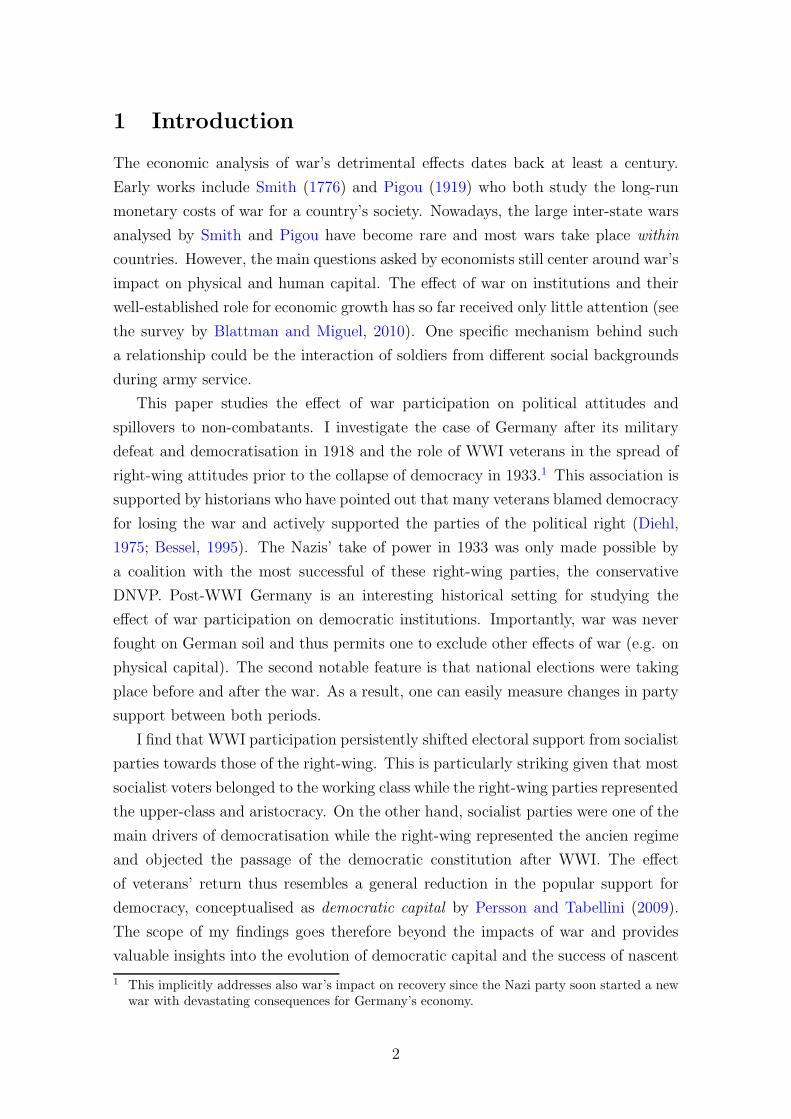
This paper studies the effect of war participation on political attitudes and

spillovers to non-combatants. I investigate the case of Germany after its military

defeat and democratisation in 1918 and the role of WWI veterans in the spread of

right-wing attitudes prior to the collapse of democracy in 1933.1 This association is

supported by historians who have pointed out that many veterans blamed democracy

for losing the war and actively supported the parties of the political right (Diehl,

1975; Bessel, 1995). The Nazis’ take of power in 1933 was only made possible by

a coalition with the most successful of these right-wing parties, the conservative

DNVP. Post-WWI Germany is an interesting historical setting for studying the

effect of war participation on democratic institutions. Importantly, war was never

fought on German soil and thus permits one to exclude other effects of war (e.g. on

physical capital). The second notable feature is that national elections were taking

place before and after the war. As a result, one can easily measure changes in party

support between both periods.

I find that WWI participation persistently shifted electoral support from socialist

parties towards those of the right-wing. This is particularly striking given that most

socialist voters belonged to the working class while the right-wing parties represented

the upper-class and aristocracy. On the other hand, socialist parties were one of the

main drivers of democratisation while the right-wing represented the ancien regime

and objected the passage of the democratic constitution after WWI. The effect

of veterans’ return thus resembles a general reduction in the popular support for

democracy, conceptualised as democratic capital by Persson and Tabellini (2009).

The scope of my findings goes therefore beyond the impacts of war and provides

valuable insights into the evolution of democratic capital and the success of nascent

1 This implicitly addresses also war’s impact on recovery since the Nazi party soon started a newwar with devastating consequences for Germany’s economy.

2

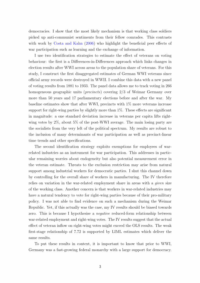
democracies. I show that the most likely mechanism is that working class soldiers

picked up anti-communist sentiments from their fellow comrades. This contrasts

with work by Costa and Kahn (2006) who highlight the beneficial peer effects of

war participation such as learning and the exchange of information.

I use two identification strategies to estimate the effect of veterans on voting

behaviour: the first is a Differences-in-Differences approach which links changes in

election results after WWI across areas to the population share of veterans. For this

study, I construct the first disaggregated estimates of German WWI veterans since

official army records were destroyed in WWII. I combine this data with a new panel

of voting results from 1881 to 1933. The panel data allows me to track voting in 266

homogeneous geographic units (precincts) covering 2/3 of Weimar Germany over

more than 50 years and 17 parliamentary elections before and after the war. My

baseline estimates show that after WWI, precincts with 1% more veterans increase

support for right-wing parties by slightly more than 1%. These effects are significant

in magnitude: a one standard deviation increase in veterans per capita lifts right-

wing votes by 2%, about 5% of the post-WWI average. The main losing party are

the socialists from the very left of the political spectrum. My results are robust to

the inclusion of many determinants of war participation as well as precinct-linear

time trends and other specifications.

The second identification strategy exploits exemptions for employees of war-

related industries as an instrument for war participation. This addresses in partic-

ular remaining worries about endogeneity but also potential measurement error in

the veteran estimate. Threats to the exclusion restriction may arise from natural

support among industrial workers for democratic parties. I shut this channel down

by controlling for the overall share of workers in manufacturing. The IV therefore

relies on variation in the war-related employment share in areas with a given size

of the working class. Another concern is that workers in war-related industries may

have a natural tendency to vote for right-wing parties because of their pro-military

policy. I was not able to find evidence on such a mechanism during the Weimar

Republic. Yet, if this actually was the case, my IV results should be biased towards

zero. This is because I hypothesise a negative reduced-form relationship between

war-related employment and right-wing votes. The IV results suggest that the actual

effect of veteran inflow on right-wing votes might exceed the OLS results. The weak

first-stage relationship of 7.72 is supported by LIML estimates which deliver the

same results.

To put these results in context, it is important to know that prior to WWI,

Germany was a fast-growing federal monarchy with a large support for democracy.

3

Even though national elections were not significant, votes for democratic parties

reached about 77% in 1912. Upon facing defeat in 1918, army mutinies ended the

war by turning Germany into a democracy. After the transition, coup attempts and

economic crises quickly led to a dramatic fall in support for democratic parties. This

trend continued when the Great Depression hit Germany in 1930. Three years later,

the anti-semitic Nazi party formed a coalition government with the conservative,

anti-democratic German National People’s Party (DNVP) which ended democracy

and the Weimar Republic. In fact, the positive impact of veterans on right-wing

parties is mainly favouring the DNVP rather than the Nazi party. There is, however,

an important difference in the timing of this effect. Losses of the socialists due to

war participation can already be observed in 1920. The beneficiaries at this point,

however, are scattered over the whole party spectrum. In May 1924 – more than 5

years after WWI – these effects disappear and war participation starts to exclusively

benefit the right-wing. Once materialised, both effects are highly persistent and last

until the final Weimar election in 1933. Without any prior assumption, this timing

suggests that the effect on socialists was related to war participation while the second

one originated from the post-war period.

The paper investigates several channels through which war participation may

affect political attitudes. Using data on veteran benefit recipients, I can rule out

that impoverishment or exposure to violence are driving the results. Rather, my

findings are in line with the spread of an anti-communist conspiracy theory, the

stab-in-the-back myth, which soldiers from the working class could have picked up

during their army service. This conspiracy theory was spread by reactionary, right-

wing circles and conveyed the message that democratic parties had betrayed the

German population and were planning to surrender Germany to Bolshevism. I find

that the effect was highest in precincts with a large share of the working class which

narrows down the attention to this part of the society. Pre-WWI militarism, religion,

and age composition of WWI eligible cohorts do not have any explanatory power.

Two events between 1920 and 1924 could explain the observed timing of the

swing to the right: politicisation of veteran associations and the radicalisation of the

German Communists. In order to assess the first channel, I hand-collected, digitised,

and geo-coded archival data on members of the three main political veteran associ-

ations in the Weimar Republic. Using this data, I can show that organised veterans

do not explain my findings. Anti-communism, on the other hand, is supported by

two different results. First, I demonstrate that veterans’ effect on voting is mainly

originating from areas with a comparatively high share of Communist votes. The

second test uses the establishment of anti-communist paramilitary volunteer units

4

(Freikorps) between 1918 and 1923. I digitised and geo-coded a comprehensive

list of Freikorps paramilitaries which allows calculating each precinct’s proximity to

the nearest unit. My findings suggest that areas located closer to anti-communist

volunteer units show a significant effect of veterans on voting.

Having narrowed down the attention to anti-communism among the working

class, I continue by exploring the transmission to veterans and from them to others.

In my analysis, I provide evidence that the effect was not only larger in working

class areas but also restricted to those where exposure to ideologies different from

socialism was particularly low. This is compatible with the idea that interaction of

soldiers from different social backgrounds during wartime were particularly helpful at

injecting new political ideas into a formerly secluded part of society – anti-communist

in this case. In order to restrict the focus further to interaction among soldiers rather

than soldiers and their superiors, I digitised a military census from 1906 which gives

me data on the recruiting patterns of the German officers corps. Using this data, I

do not find any proof for a specific role of sergeants and other high-rank militaries.

Finally, I explore settings under which veterans could have passed their thoughts on

to others. I provide evidence which makes a transmission through the family network

and to spouses appear unlikely. Rather, transmission seems to be conditional on high

political competition in May 1924.

This paper contributes to the economic literature on the effects of war partici-

pation. Seminal research in this area is Angrist (1990) who estimates the negative

impact of military service on earnings of U.S. veterans. Angrist’s study has been

followed by numerous related work on the effects of war participation in the field of

labour economics.2 Evidence on the social or political effects of war participation has

attracted less attention. One of these are Costa and Kahn (2006) who demonstrate

how ex-slaves serving in the Union Army systematically benefited from a diverse unit

by learning from their peers. In general, war experience seems to help overcoming

collective action problems (see the studies by Jha and Wilkinson, 2012; Campante

and Yanagizawa-Drott, 2015). Regarding the political outcomes, Blattman (2009)

finds higher political activity among child combatants in Uganda while Grossman,

Manekin, and Miodownik (2015) shows that Israeli recruits’ exposure to violence

lowered combatants’ willingness to seek reconciliation and increased support for

2 Recent work on Vietnam veterans includes Angrist, Chen, and Song (2011) and Angrist andChen (2011). There is also a literature on the consequences of participation in civil war (seefor example Humphreys and Weinstein, 2007; Annan and Blattman, 2010; Gilligan, Mvukiyehe,and Samii, 2013).

5

parties of the political right.3 Similar to Grossman, Manekin, and Miodownik, I

argue for a negative impact of war participation. The main mechanism, however, is

not exposure to violence but rather interaction with peers in the spirit of Costa and

Kahn.

My findings also speak to the study of war’s long-run impacts. Researchers

until now have mostly looked at physical and human capital destruction. Regarding

political outcomes, Bellows and Miguel (2009) show that war violence led to higher

political activity in affected households. Institutional aspects are only addressed by

Acemoglu, Hassan, and Robinson (2011) who find that the systematic murder of

middle-class Jews during the Holocaust in WWII had persistent negative effects on

economic and political progress in Russian cities. I add to this literature in two ways.

On the one hand, this is one of few investigations into the still open question of war’s

effects on institutions (Blattman and Miguel, 2010). Secondly, my results suggest

that, even if fought abroad, war can have negative consequences in the belligerent

country through the transmission of detrimental political ideas. The persistent

shift of votes from democratic to anti-democratic parties relates my work to the

study of democratic capital, people’s intrinsic valuation of democracy. Pioneered

by Persson and Tabellini (2009), the determinants of democratic capital have also

been evaluated empirically in a number of recent studies (Giuliano and Nunn, 2013;

Grosfeld and Zhuravskaya, 2015). While most of these are looking at long-run

institutional determinants, my study documents short-run changes in democratic

capital due to human interactions. I also find evidence for the transmission of

democratic values to others which has recently been conceptualised theoretically by

Ticchi, Verdier, and Vindigni (2013).

Finally, this paper also contributes to the growing quantitative literature on the

rise of the Nazi party in economic history and political economy. King et al. (2008)

and Bromhead, Eichengreen, and O’Rourke (2013) relate the Great Depression to

the rise of authoritarianism during the 1920s and 1930s in Germany and other

countries. My paper focusses on the role of the post-war period and societal factors

behind this development. Voigtlander and Voth (2012) demonstrate how anti-semitic

attitudes from past centuries sparked up again after WWI and supported the rise

of the Nazi party. Satyanath, Voigtlander, and Voth (forthcoming), on the other

hand, investigate the role of civic associations as tool for the Nazi party to infiltrate

society. Crucially for my study, the authors also compare the effects of military and

non-military associations but do not find evidence for a particular role of veterans’

3 Erikson and Stoker (2011) use the Vietnam draft lottery status to estimate the effect of becomingdraft-eligible – as opposed to being drafted – on political attitudes. They show that draftvulnerability persistently increased anti-war and liberal attitudes among young men.

6

associations in recruiting members for the Nazi party. I second these findings using

data on membership strengths of military associations. To the best of my knowledge,

my paper is the first to empirically investigate the role of WWI veterans as well

as the general success of anti-democratic, right-wing parties during the Weimar

Republic. Rather than the Nazi party itself, I find that veterans were benefiting

the like-minded but less prominent DNVP which played a crucial role in making

Adolf Hitler Germany’s Chancellor in 1933. I am also the first to empirically link

the activity of German Communists in the 1920s to the rise of right-wing support.

The rest of the paper proceeds as follows: Section 2 provides the reader with

important historical background on Weimar democracy, the role of the former WWI

soldiers therein, and the stab-in-the-back myth. In section 3 I give a detailed

description of how the veteran estimate as well as the election panel dataset are

constructed. Section 4 outlines the empirical strategies applied in this paper. Next,

section 5 presents the main empirical results and and a number of robustness

checks. Section 6 investigates the mechanisms underlying the baseline effect. Finally,

section 7 concludes.

2 Historical background

2.1 World War I, the stab-in-the-back myth and the demo-

cratisation of Germany

Germany’s path towards democracy reaches back as far as 1848 when a provisional

national assembly was gathered in order to design a constitution for a still to

be unified Germany. This democratic experiment was crushed soon afterwards

leading to a period of restoration until Prussia’s victory over France in 1871 resulted

in the proclamation of the German Empire. It was a constitutional monarchy

under Prussia’s leadership that for the first time introduced a publicly elected

parliament on German territory. Even though its competencies were limited at

first, the Reichstag ’s role increased as it had to approve the Empire’s budget which

became particularly important during WWI and the preceding arms build-up. Under

Emperor Wilhelm II, the German Empire had started a period of unpredictable and

provocative foreign policy which isolated it from most of its former European allies,

most notably Russia and the United Kingdom. As a result, it took only a spark in

form of the assassination of Archduke Franz Ferdinand of Austria to start the First

World War on 28th of July 1914.

7

Even though the German Empire was quite successful at the beginning of the

campaign, the progress at the western front came to a halt at the end of 1914 and

was followed by four-year war of attrition with the highest death toll experienced

until that point. By the end of September 1918, the situation of the German Army

had deteriorated to such an extent that the Supreme Army Command (Oberste

Heeresleitung) admitted defeat to the Emperor. A new grand government including

members of the social democratic party was formed subsequently and few days

later, US President Woodrow Wilson was officially asked for an armistice. When

the Supreme Army Command rejected the conditions set by the Allied Forces in late

October 1918, Chancellor von Baden sacked the leadership of the Supreme Army

Command and issued political reforms which turned Germany into a parliamentary

monarchy. The war, however, continued until the end of October when a mutiny

by the German Navy in Kiel sparked a rebellion and the formation of socialist

workers’ and soldiers’ councils. This rebellion quickly spread across the whole

German Empire and eventually led to the proclamation of the German Republic

and the abdication of Emperor Wilhelm II on the 9th of November (Buttner, 2008).

World War I officially ended two days later with the signing of an armistice.4

One of the key reasons for Weimar democracy’s failure 15 years later was that

the German Army was still fighting when the armistice was signed. This soon gave

rise to the stab-in-the-back myth, a conspiracy theory according to which Germany

had not lost World War I but was stabbed in the back by socialist and Jewish

politicians and their supporters. The fact that social-democrats inherited power as

the strongest parliamentary group and its ally, the left-liberal DDP, was traditionally

popular among the Jewish population provided the material to fabricate a lie which

many – especially militarists, monarchists as well as followers of the anti-semitic

Volkisch movement – “wanted to believe” (Bessel, 1988). The new state was therefore

discredited from its very beginning as a project of unpatriotic cowards which made

it very hard for large parts of the society to identify with the new democratic

republic. This was further facilitated by a number of socialist rebellions which spread

fear among the population of a violent October Revolution-style coup – allegedly

tolerated or encouraged by the parties of the centre and left (Merz, 1995).

4 One may question whether this transition can in fact be regarded as a democratisation. WhileImperial Germany was not a full-blown autocracy, its constitution did not put any constraintson the executive and is therefore placed in the grey zone between democracy and dictatorshipin 1914 on the POLITY scale (-10 to +10) with a value of 2 (Jaggers and Marshall, 2014).This ambivalence also been noted by other scholars (Jesse, 2013). After 1918, the power ofthe executive is bounded and the POLITY indicator jumps to a value of 6 where it remainsuntil 1933. One can thus safely say that the revolution of 1918 resulted in a higher degree ofdemocracy despite the unclear point of departure. Further arguments why 1918 can be regardedas a democratisation are reflected in the opinions voiced by its opponents in sectionA.1

8

The stab-in-the-back myth can be regarded as the key mechanism for transmit-

ting anti-democratic thought and eroding democratic capital during the Weimar

Republic (Barth, 2003). While being spread through various social groups such

as paramilitaries or universities, there were only two main parties of the Weimar

Republic who were more or less openly propagating its content and spreading right-

wing anti-democratic sentiments. These were the extremely anti-semitic Nazi party

NSDAP, including its predecessors, and the national-conservative German National

People’s Party DNVP (Mommsen, 1996).

2.2 WWI veterans’ role during Weimar democracy

As highlighted by several authors, not all veterans were anti-democratic or right-

wing. Those who became politically active and claimed to represent the front

generation, however, were in great majority on the extreme right of the political

spectrum (Diehl, 1975; Bessel, 1995). Paramilitary units founded in the war’s

aftermath were officially disbanded in 1923, but continued to exist in non-military

cover organisations or within right-wing veteran associations like the Stahlhelm

(Buttner, 2008). Membership in organisations could thus be an important mode

of veterans interacting with the society and through which voting behaviour could

be influenced. As highlighted by Anheier (2003) for the Munich chapter of the

Nazi party, anti-democratic activists tended to hold co-memberships in several

paramilitary units, racist clubs, and political parties. While it is not possible to

investigate each of them, my analysis of the channel focusses on ex-servicemen

clubs since they had a clear political distinction and are one the few types of such

organisations for which membership data has survived in archives.5

Joining one of many veteran associations was not only popular among anti-

democratic veterans as membership numbers of the rightist Stahlhelm (500,000), the

(social) democratic Reichsbanner (1,000,000) and the Communist Rotfront (150,000)

show (Ziemann, 1998). Officially, those associations were not very political but

rather meeting places for former soldiers of a specific social background to relive

and commemorate their front experiences. Some members of these associations were

also running as candidates in elections and veteran associations were very active in

supporting the campaign of their favourite parties (Ziemann, 2013). The Stahlhelm

was initially loosely aligned with the conservative liberal, yet democratic, DVP

and the authoritarian DNVP. However, the strong aversion against liberalism and

socialism made it embrace soon also members of the anti-democratic paramilitary as

5 Anheier (2003), for instance, provides an informative quick overview of the main types oforganisations joined by radicalised veterans.

9

well as anti-semitic extremists. In December 1924, the Stahlhelm started to openly

support the nationalist parties in helping to organise rallies and organise marches

(Klotzbucher, 1965). Shortly afterwards, the Stahlhelm had turned into a political

combat league and strongly involved in the increasing political violence between left

and right (Berghahn, 1966). The increasing political role of the veteran associations,

was also recognized by politicians:

“Since 1924 a change has been noticeable. (...) The organizations no

longer – or no longer exclusively – limit themselves to the field of soldierly

activity, but increasingly are becoming engaged in the political struggle

and are seeking to obtain political influence and political power (...).”

Albert Grzezinski (Prussian Minister of the Interior), quoted in Diehl

(1975, p.173)

As the preceding sections have shown, veterans started to get politicised during the

transition period especially where the new state was weak, threatened by uprisings

and the need to rely on right-wing paramilitary was high. Anecdotal evidence

has also highlighted the elevated role of soldiers within German society and the

increasing political power of ex-servicemen clubs as potential mechanisms through

which soldiers could have influenced right-wing attitudes. The following section

describes the construction and collection of the data used to analyse veterans’ effect

on political attitudes.

3 Data

3.1 Estimating Germany’s World War I veterans

The data section starts by describing how I estimated the amount of German WWI

veterans. Collecting data on German WWI soldiers is a challenging task since

almost all primary material from the German Army Archive has been destroyed in

an air raid during Second World War. This makes statistical data the only source

to recover reliable information on WWI participation in the German Empire. The

starting point is the exact number of soldiers having served in the German Imperial

Army during 1914 and 1918 and not dying, Veterans. This number is transformed

into a treatment intensity Veterans per cap.. The base population is taken from the

10

1910 census which gives the last reliable counts unaffected by WWI.6 In order to

save on notation, the term per cap. is omitted in the remainder of this section:

Veterans = Soldiers1913 +1918∑

t=1914

SoldiersJoint −

1918∑

t=1914

SoldiersDeadt (1)

Unfortunately, the components of this ideal measure are not readily available at a

disaggregated level and veterans as such were also never subject of any statistical

publication.7 However, I will show that they can be estimated quite accurately

with census data and are congruent with aggregate numbers from official sources.8

The main data used in this study are two mid-war censuses conducted by the

Office of War Nourishment’s Economic Department (Volkswirtschaftliche Abteilung

des Kriegsernahrungsamtes) in December 1916 and 1917 as well as the first post-

war census in October 1919.9 The December 1917 census contains county level

numbers on the amount of military persons present at the time of the census,

SoldiersHome1917. The main problem is that soldiers serving in December 1917

were omitted from the census.10 The way I resolve this issue is exploiting the

fact that only men served in the army. This shows up as a notable gender gap

in the mid-war censuses but crucially also in a considerably different population

growth between women and men from 1917 to 1919.11 Taking the gender-difference

in population growth gives an estimate of men absent between 1917 and 1919,

henceforth MissingMen1917−1919:12 This measure is, however, also driven by gender-

specific differences in births, civilian deaths and migration. The first two can be

estimated and are discussed in section D.1 in the appendix. Differences in migration

6 An alternative way of doing this, would be using the population from the first post-war censuscarried out in October 1919, about a year after the armistice of 11th November 1918. However,since the latter may be endogenous due to post-WWI migration, pre-war population seems asomewhat safer choice.

7 An exception is the statistic of recipients of war-related benefits on 1929 which however coversless than 60,000 of the 11 million surviving German WWI participants and to which also widowsand orphans were entitled. A per capita measure of benefit recipients is weakly negativelycorrelated with my measure of veterans at −0.08.

8 See section D.3 for details.9 According to Bessel (1993), a large amount of the 800,000 German prisoners of war had returned

by late 1919.10 The equivalent census at the front did not collect data on soldiers’ residence and could thus not

be matched with the county level data. This practice was severely criticised among Germany’sstatisticians (Bayerisches Statistisches Landesamt, 1919).

11 Prisoners of war were also counted as local population in mid-war censuses and have beenremoved from Male1917.

12 Further details on this calculation are provided in the appendix.

11

cannot be estimated and deducted and have to be accounted for by controlling for

gender-specific migration 1910–1919.

Apart from gender-differences the sum of SoldiersHome1917 andMissingMen1917−1919

does also not account for fluctuations in and out of the army before and after

December 1917. Dead soldiers are not problematic since neither those who die before

or after 1917 are counted. However, a considerable number of soldiers had left the

army before December 1917 for other reasons than death while others were still to

join until the end of the war. Since age and desertion can be deemed negligible,

those leaving the army alive should be roughly equivalent to the amount of severely

wounded soldiers.13 I thus also make use of a preliminary, unofficial version of the

December 1916 census. This provides me with county-level data on war-disabled

members of the German army. Disaggregated numbers on the 700,000 men who had

left the army due to injury between 1916 and 1917 or were still to join the army in

1918 could not be retrieved (Statistisches Reichsamt, 1926). These will be part of the

composite measurement error discussed in section 4.1. Adding WarDisabled1916 to

the sum of SoldiersHome1917 and a gender-corrected version of MissingMen1917−1919

completes the veteran estimate used in this study:

˜Veterans =SoldiersHome1917 +MissingMen1917−1919

− (Male Births1917−1919 − Female Births1917−1919)

+ (Male CivilDeaths1917−1919 − Female Deaths1917−1919)

+WarDisabled1916

(2)

The density of the normalised estimate ˜Veterans is depicted in figure 1. One can

see that it is almost bell-shaped and ranging between 4 and 19% with a mean

and median of 14% and 13.7%, respectively. Remaining issues about the veteran

estimate such as measurement error and endogeneity will be discussed in further

detail in section 4.1.

3.2 Panel data of Reichstag elections 1881−1933

In order to track changes in precincts’ voting behaviour over time, I compiled a panel

dataset covering 17 parliamentary elections held between 1881 and Hitler coming

to power in 1933. The panel is based on two existing datasets on elections in

13 The study by Jahr (1998) estimates that no more than 50,000 out of almost 13 million Germansoldiers deserted. The rule of dropping out for leaving the conscripted age group between 17and 45 was suspended in the German army during the First World War (Nash, 1977).

12

Figure 1: Density of veteran inflow per capita

0

10

20

0.05 0.10 0.15 0.20

Veterans per cap. 1910

Density

Imperial and Weimar Germany from ICPSR (1991) and Falter and Hanisch (1990),

respectively. All voting data were initially taken from original publications by the

German (Imperial) Statistical Office. A dataset comparing election results over

almost 60 years, however, raises important issues regarding the units of analysis as

well as the changes in Germany’s party system.

While the issue of area redistricting is discussed in section 3.3, the second major

concern is the comparability of parties across time. A brief look into the history

of the NSDAP illustrates this very well: during the German Empire there was no

anti-semitic party of mass support but only various like-minded splinter parties

such as the Deutsch Reformpartei (German Reform Party) or the Wirtschaftliche

Vereinigung (Economic Union). The Nazi party was eventually founded under the

name of the Deutsche Arbeiterpartei (DAP, German Workers’ Party) in 1918 and

changed its name into NSDAP (National-Socialist German Workers’ Party) in 1920.

After Hitler’s first coup attempt in 1923 the party was banned and leading members

of the NSDAP joined forces with the Deutsch-Volkische Freiheitspartei (German

Volkisch Freedom Party, DVFP). From 1924 onwards, when it became re-allowed,

the NSDAP became quickly the largest anti-semitic party.

This development is exemplary for almost any part of Germany’s political spec-

trum and highlights the need for a more stable categorisation which accounts for

13

Figure 2: Long-term evolution of election results 1881-1933 (WWI start/end, solid lines; pre/post-WWI elections, dashed lines)

Rightwing Centre

Liberal Socialist

0.0

0.2

0.4

0.6

0.0

0.2

0.4

0.6

1881

1884

1887

1890

1893

1898

1903

1907

1912

1920

1924

1928

1930

19

33

1881

1884

1887

1890

1893

1898

1903

1907

1912

1920

1924

1928

1930

19

33

1881

1884

1887

1890

1893

1898

1903

1907

1912

1920

1924

1928

1930

19

33

1881

1884

1887

1890

1893

1898

1903

1907

1912

1920

1924

1928

1930

19

33

1881

1884

1887

1890

1893

1898

1903

1907

1912

1920

1924

1928

1930

19

33

1881

1884

1887

1890

1893

1898

1903

1907

1912

1920

1924

1928

1930

19

33

1881

1884

1887

1890

1893

1898

1903

1907

1912

1920

1924

1928

1930

19

33

1881

1884

1887

1890

1893

1898

1903

1907

1912

1920

1924

1928

1930

19

33

1881

1884

1887

1890

1893

1898

1903

1907

1912

1920

1924

1928

1930

19

33

1881

1884

1887

1890

1893

1898

1903

1907

1912

1920

1924

1928

1930

19

33

1881

1884

1887

1890

1893

1898

1903

1907

1912

1920

1924

1928

1930

19

33

1881

1884

1887

1890

1893

1898

1903

1907

1912

1920

1924

1928

1930

19

33

1881

1884

1887

1890

1893

1898

1903

1907

1912

1920

1924

1928

1930

19

33

1881

1884

1887

1890

1893

1898

1903

1907

1912

1920

1924

1928

1930

19

33

1881

1884

1887

1890

1893

1898

1903

1907

1912

1920

1924

1928

1930

19

33

1881

1884

1887

1890

1893

1898

1903

1907

1912

1920

1924

1928

1930

19

33

1881

1884

1887

1890

1893

1898

1903

1907

1912

1920

1924

1928

1930

19

33

1881

1884

1887

1890

1893

1898

1903

1907

1912

1920

1924

1928

1930

19

33

1881

1884

1887

1890

1893

1898

1903

1907

1912

1920

1924

1928

1930

19

33

1881

1884

1887

1890

1893

1898

1903

1907

1912

1920

1924

1928

1930

19

33

1881

1884

1887

1890

1893

1898

1903

1907

1912

1920

1924

1928

1930

19

33

1881

1884

1887

1890

1893

1898

1903

1907

1912

1920

1924

1928

1930

19

33

1881

1884

1887

1890

1893

1898

1903

1907

1912

1920

1924

1928

1930

19

33

1881

1884

1887

1890

1893

1898

1903

1907

1912

1920

1924

1928

1930

19

33

1881

1884

1887

1890

1893

1898

1903

1907

1912

1920

1924

1928

1930

19

33

1881

1884

1887

1890

1893

1898

1903

1907

1912

1920

1924

1928

1930

19

33

1881

1884

1887

1890

1893

1898

1903

1907

1912

1920

1924

1928

1930

19

33

1881

1884

1887

1890

1893

1898

1903

1907

1912

1920

1924

1928

1930

19

33

1881

1884

1887

1890

1893

1898

1903

1907

1912

1920

1924

1928

1930

19

33

1881

1884

1887

1890

1893

1898

1903

1907

1912

1920

1924

1928

1930

19

33

1881

1884

1887

1890

1893

1898

1903

1907

1912

1920

1924

1928

1930

19

33

1881

1884

1887

1890

1893

1898

1903

1907

1912

1920

1924

1928

1930

19

33

14

the various name changes, mergers and splits in order to analyse long-term trends.

I am relying on an established classification used in the study of historical German

parties augmented by a separate category for anti-semitic groupings (Jesse, 2013): 1)

Anti-semitic; 2) (Protestant) Conservative; 3) Right-Liberals; 4) (Catholic) Centre;

5) Left-Liberals; 6) Socialist; 7) Agrarian/Particularist (Others).14 The individual

parties’ votes are aggregated to their closest fit in the political spectrum and treated

as quasi parties existing over the whole period of interest. The aggregates are

then divided by the amount of total ballots cast in order to obtain vote shares.

In the Weimar Republic, the main protagonists actively opposing democracy were

Antisemitic, Conservative, and Right-Liberals.15 My main outcome is the combined

vote share of these three parties which I call Right-wing. The socialist party split

during WWI into social democrats and Communists. I continue to use their sum as

socialist votes after WWI to ensure comparability. In one specification I also add

Communist votes to the Right-wing which gives Non-democratic votes.

Figure 2 shows the aggregate voting data by political party over the used sample.

What is remarkable is the stability of right-wing votes until the end of WWI and

the sudden steep rise shortly after. While the centre parties remained very stable

throughout this sixty years period, the results of liberals and social democrats show

where the right-wing shares were coming from. Liberal votes had stabilised at about

20% until the war and then started to fall gradually to significantly below 10% in

1933. Socialist votes did not experience such a downturn but saw their clear upward

trend during the German Empire come to a sudden halt during the 1920s and 1930s.

3.3 Construction of panel and control variables

This section describes the construction of the dataset and remaining control vari-

ables. The core of my dataset is a unique panel covering 17 parliamentary elections

held between 1881 and Hitler coming to power in 1933. A panel over more than

60 years, however, requires stable units of analysis not only for the electoral results

but also all other data to be merged to it. While most current work on Weimar

14 An alternative classification is the one by Sperber (1997) who treats Anti-semitic and Conserva-tive as a single conservative bloc and assigns the Centre party to the Agrarians/Particularists.

15 Counting the right-liberals as right-wing is not straightforward. The main reasons are twofold:first, they were involved in many pre-election agreements with the conservatives during theGerman Empire which makes their vote shares difficult to separate. Second, despite participatingin many governments the DVP opposed the draft of the post-war constitution and had manylinks to right-wing organisations such as the Stahlhelm. The DNVP also joined governmentduring 1925 and 1927/1928, but research shows that this did not alter the party’s general anti-democratic position. In fact, the party chairman Count Westarp was removed from office in 1928because he refused to exclude a member urging for the acceptance of the Republic (Buttner,2008; Gasteiger, 2014).

15

Germany uses data at the city or county level, voting results during the German

Empire were only published for each precinct. This unit was solely used for electoral

purposes and only few exceptions followed political boundaries, e.g. for very small

states and administrative districts. Each precinct typically consisted of a cluster of

2-4 counties with occasional but usually negligible overlaps. An attractive feature

of those precincts is also that for political reasons they were never adjusted for

the considerable population changes and remained stable from 1871 to 1912 (Jesse,

2013). After World War I, Germany was divided into 35 new electoral precincts of

larger but roughly equal size, but at the same time election data became published

at much finer levels of aggregation such as counties and sometimes even larger

municipalities. The smallest units of analysis with data available for pre- and post-

WWI are thus the 397 former Imperial precincts. 16

The counties they consisted of, however, were subject to frequent changes such

as mergers, partial incorporations and splits. Hence, in a first step I coded all county

reforms during the respective time period and constructed a set of stable counties.

These are counties that existed at one point in time but where district reforms

happened in such a way that numbers for the stable county can be reconstructed from

adding up data of past or future sets of counties. If I was also able to re-construct

the area of a whole precinct by adding up stable counties or if they coincided, this

precinct was included in my dataset. In doing so, I was able to recover 266 out of

the 397 Imperial precincts. About a quarter of the missing areas were from Alsace-

Lorraine and Posen/West Prussia ceded to France and Poland after World War I.

Another third is from densely populated – and often re-districted – agglomerations

such as the Ruhrgebiet and very large cities with several precincts such as Berlin or

Munich.

For this study I collected and digitised a number of additional data. One

exception is the digitised Prussian version of the 1910 census which was taken from

Galloway (2007). To start with I digitised the German census of 1910 which provides

me with data on religion and population size. I include population share of catholics

and protestants and log(population) as controls variables. The 1910 census also

provides me with the last pre-WWI data on cohort size by gender. Unfortunately,

the latter are only reported in very large groups and does not allow to infer male

cohorts born between 1869 to 1901 and thus eligible for WWI. I therefore use the far

more detailed publication of the census results for Prussian population provided in

(Galloway, 2007). Together with data from the 1916 census this gives me the size of

the male cohorts born 1869–1901 for about half my sample. In a two-step procedure

16 For the remainder of this paper, precincts is referring to those of Imperial Germany.

16

I use this data to predict the cohort size 1869–1901 for the whole sample.17 I also

collected vital statistics for the German Empire for the time period 1910 to 1919

at the level of counties and administrative districts. I use this data to correct for

gender-differences in MissingMen1917−1919 and to calculate gender-specific migration

between 1910–1919 and infant mortality in 1912.18

I also digitised the occupational census of 1882 which provides me with detailed

county information on peoples’ profession. From this I can calculate the share of

the population working in manufacturing and in war-related industries. The latter

forms my instrumental variable for war participation and is described in more detail

in section 4.3. Finally, I control for turnout by dividing the amount of total votes

by the size of the electorate. All control variables are at the cross-sectional level

and included in the regression by interacting them with election fixed-effects. For

the sake of brevity, I do not introduce them at this point but in the respective

subsections of 6. I use a number of other variables in my mechanism analysis in

section 6. Summary statistics for all variables relevant to the baseline specifications

are reported in table 1.

17 First, I run a simple regression of the actual cohort size 1869/1901 on the limited set of variablesavailable from the all-German results. I then use these estimated coefficients to predict cohortsize 1869/1901 for the rest of the sample

18 I add perinatal births in 1912 to deaths within first-year of 1913 and divide by births in 1912.

17

Table 1: Descriptive statistics

Obs Mean Std.Dev. Min Max

Veteran-relatedVeterans per cap. 266 0.14 0.02 0.05 0.19Population 1910 in 1,000 266 152.50 106.90 24.16 937.38

Socio-economic% Protestants 1910 266 0.64 0.36 0.00 1.00% Catholics 1910 266 0.34 0.36 0.00 1.00% Infant mortality 1912 266 0.17 0.04 0.09 0.31% Working in manufacturing 1882 266 0.13 0.05 0.04 0.31% Working in war industries 1882 266 0.02 0.02 0.01 0.17% WWI eligible men (born 1969-1901) 266 0.29 0.01 0.24 0.35% ∆Male migration 1910-1919 266 −0.03 0.01 −0.09 0.02

Voting% Turnout 4, 522 0.75 0.12 0.20 0.95% Vote Anti-semitic 4, 522 0.10 0.17 0.00 0.79% Vote Conservative 4, 522 0.19 0.21 0.00 0.99% Vote Right-Liberal 4, 522 0.11 0.16 0.00 0.97% Vote Centre 4, 522 0.23 0.29 0.00 1.00% Vote Left-Liberal 4, 522 0.10 0.15 0.00 0.91% Vote Socialist 4, 522 0.23 0.17 0.00 0.71% Vote Communist (post-WWI) 2, 128 0.08 0.06 0.00 0.33% Vote Others 4, 522 0.04 0.09 0.00 0.75

Notes: The unit of observation is one of the 266 precincts in the sample at election t. Variablesprovided at the cross-sectional level only are reported accordingly and used in the analysis byinteracting them with either a post-WWI dummy or election fixed effects.

4 Identification strategy

4.1 Determinants of veteran inflow

In this subsection, I investigate the main drivers of war participation in Germany

and I ensure that the treatment assignment is plausibly random conditional on

observables. The main drivers of war participation across the German Empire were

originating from the WWI conscription system. According to the law, all men aged

17 to 45 were liable to serve in the army and the share of male cohorts 1869 to

1901 is thus expected to be one of the main factors (Nash, 1977). I include an

estimate of this cohort relative to the 1910 population interacted with a post-WWI

dummy into my set of control variables. Not all men in the relevant age groups,

however, actually had to serve and a considerable amount was exempted. Being

judged permanently unfit to fight was one main reason for exemption and at least

at the beginning of the 20th century this decision was not entirely impartial but

18

Table 2: Determinants of veteran inflow

Veterans p.c.

(1) (2) (3) (4) (5)∆Male migration1910−1919 −0.035 0.080 0.091 0.144∗

(0.073) (0.084) (0.077) (0.074)1910 share of male cohorts 1869-1901 0.283∗∗ 0.318∗∗ 0.192 0.358∗∗∗

(0.113) (0.134) (0.135) (0.120)1882 share manufacturing −0.034 −0.032 −0.085∗∗∗ −0.001

(0.023) (0.023) (0.024) (0.028)1882 share war-industries −0.332∗∗∗

(0.117)Infant mortality rate 1912 −0.002 −0.001

(0.032) (0.029)

Controls N N N Y Y

Observations 266 266 266 266 266

R2 0.001 0.046 0.050 0.185 0.271

Notes: Robust standard errors in parantheses, ∗p<0.1; ∗∗p<0.05; ∗∗∗p<0.01; Controls:Log(population) 1910; % Protestants 1910; % Catholics 1910; % New male voters post-WWI

allegedly also by factors such as parents’ occupation and living location.19 Data

on conscription in the German Empire is only available before the war but does

not corroborate such claims. The percentage of permanently unfit within the 1913

class, for example, ranged only between 4.3 and 5.9% across Germany’s 25 military

districts. During the war, these numbers were presumably even lower and more equal

since a law from September 1915 allowed re-examining everyone judged unfit before.

The intense battle for manpower (Feldman, 1966) during WWI in Germany makes

it unlikely that political concerns of the commissions could have been a systematic

driver of war participation.

The second part of exemptions was related to workers needed in war or war-

related production. By the year 1918, about 1.3 million men – a sixth of the actual

army size – was absorbed in such a way from the front to work in the factories

and mines. War participation is thus expected to be significantly lower in areas

employing a large share of men in the following industries: mining; iron and metal

processing; production of iron, metal, and steel; construction of machines, tools, and

vehicles; electrical, precision, and optical engineering.20 This share is a confounder

since it is highly correlated with the size of the working class which was at the

19 The reason behind this was the army’s general suspicion against the working class of supportingsocial democracy and being politically illoyal. See Brentano and Kuczynski (1900) and May(1917) for further discussions of this topic.

20 This classification is taken from Kocka (1978).

19

same time also the main stronghold of the social democrats. Male employment in

war industries is therefore expected to negatively affect both war participation and

right-wing votes. The IV strategy presented in section 4.3 exploits the fact that

war industries should have a direct effect on political attitudes only through the

size of the working class. My main specifications rules this channel out by including

interactions of time dummies with the employment share in manufacturing 1882.

The final determinant of the veteran estimate is mismeasurement as discussed in

section 3.1. I control for parts of this by controlling for ∆Male migration1910−1919.

Table 2 shows how the main drivers of war participation are related with my

veteran estimate. In order to casually investigate what the remaining variation may

be driven by, I construct the residuals from the specification in column (4) and plot

their spatial distribution by quartile in figure 3. Unexplained variation seems to be

slightly higher in north and south-west Germany. Reassuringly, figure 4 shows that

the correlation of the residual with pre-WWI right-wing vote shares as of 1912 is

only very weak and negative.

4.2 Differences-in-Differences

The panel structure of the data allows using unit and time fixed effects which

identifies off the within-precinct variation after accounting for time-specific trends.

In doing so, I can account for election-specific voting patterns due to candidates’

abilities, for instance, and any time-constant omitted variable. Also confounders

related to historical heritage are taken care of, given that their effect is constant over

time. My first identification strategy exploits these features and uses a difference-

in-differences methodology to investigate the level effect of veteran inflow across

German precincts on right-wing voting. The estimated equation reads as follows:

yit = α + γi + λt + βt(veteransi × postWWIt) + µX it + ǫit (3)

In the baseline model, I regress vote shares yit one the election and precinct fixed

effects γi and λt as well as a set of control variables X it which is identical to the

full set of variables in column 4 of table 2. The main variable of interest is the

interaction of the one-time treatment intensity veteransi with a dummy variable

taking on value 1 for each election after WWI (starting with the one in June 1920)

and 0 otherwise. The estimated effect should thus be interpreted as an average shift

in voting patterns across all elections after the end of the war proportionate to the

estimated population share of veterans. Whether this effect is causal depends on

20

Figure 3: Residuals from table 2, column 4 across Imperial Germany’s precincts,post-WWI borders in green

Veteran inflow(residual)

1st quartile

2nd

3rd

4th

No data

Figure 4: Correlation of unexplained veteran variation and right-wing votes in1912

-0.075

-0.025

0.025

0.075

0.00 0.25 0.50 0.75 1.00

Right-wing vote share 1912

Unexpla

ined v

ariation in v

ete

ran e

stim

ate

21

Figure 5: Average rightwing vote share before/after WWI depending on veteraninflow residual (median)

0.0

0.2

0.4

0.6

1881

1881

1884

1884

1887

1887

1890

1890

1893

1893

1898

1898

1903

1903

1907

1907

1912

1912

1920

1920

1924

1924

1928

1928

1930

1930

1933

1933

1881

1881

1884

1884

1887

1887

1890

1890

1893

1893

1898

1898

1903

1903

1907

1907

1912

1912

1920

1920

1924

1924

1928

1928

1930

1930

1933

1933

1881

1881

1884

1884

1887

1887

1890

1890

1893

1893

1898

1898

1903

1903

1907

1907

1912

1912

1920

1920

1924

1924

1928

1928

1930

1930

1933

1933

1881

1881

1884

1884

1887

1887

1890

1890

1893

1893

1898

1898

1903

1903

1907

1907

1912

1912

1920

1920

1924

1924

1928

1928

1930

1930

1933

1933

1881

1881

1884

1884

1887

1887

1890

1890

1893

1893

1898

1898

1903

1903

1907

1907

1912

1912

1920

1920

1924

1924

1928

1928

1930

1930

1933

1933

Below median veteran inflow (residual)

Above (normalised to 1881)

two assumptions: the first is that areas of high and low treatment intensity follow

similar voting patterns before WWI and that the observed change is not part of a

trend starting before WWI.

I tackle this concern in several ways: the most simple one is presented in figure 5

which plots the average right-wing vote share over time for precincts with above

and below median values of the residual plotted in figure 3. As can be seen, the two

lines are diverging before the war with less-treated districts exceeding the other ones

by about 4%. After WWI, this trend reverses and by May 1924 the average votes

in both groups are almost equal. The second test uses a non-linear version of the

effect by interacting the treatment veteransi with 20 election fixed effects leaving out

1912 as the reference election. While being more demanding on the data, this allows

exploring anticipating behaviour and explicitly test the common trends assumption.

This would not be satisfied if precincts with higher treatment intensity started to

show increasingly higher voting results for anti-democratic parties already before

the war. A third alternative is the inclusion of area-specific election fixed effects

and precinct-specific time trends. Both tests are presented as a robustness check in

section 5.2.

The second necessary assumption is the absence of confounding events correlated

with both the arrival of veterans and support for the extreme right. The vector of

22

control variables Xit features several factors deemed to fulfil these criteria. Apart

from the determinants of (estimated) veteran inflow, I also include further data.

The first of these is the natural log of the population and serves as a proxy for the

precinct’s size. Unlike the percentage of new female voters, the amount of new male

voters is correlated with the treatment and thus included in the regression. New

male voters are those born between 1896 and 1900 who would have not been allowed

to vote in 1920 under the old law. I proxy this with the cohorts from 1895 to 1900

taken from the censuses 1910 and 1916 and create a new variable NewMaleV otersit

which is zero before WWI and afterwards equal to the size of the newly enfranchised

cohorts divided by the 1910 total population.

Furthermore, I include socio-economic characteristics of each precinct. In ad-

dition to the size of the working class and infant mortality, I also control for the

religious composition of precincts using the shares of Protestants and Catholics in

1910. Including religion into the specification is necessary since Protestants were

more supportive of the German Empire especially after the extremely polarising

Kulturkampf secularisation period and it is possible that war volunteering was also

higher among them. If the (predominantly Protestant) conservative parties had

started to actively fight democratisation only after the war, this would be a source

of bias. In order to include the time-invariant control variables into the fixed effect

regression, each of them is interacted with a set of election dummies. Finally, the

standard errors of the regression are clustered at the precinct level to account for

correlation of unobservable characteristics over time.

4.3 Instrumenting veteran inflow

Even though the diff-in-diff specification already controls for a range of unobserve-

ables, one should refrain from interpreting these estimates in a causal way. Many

important factors are likely to have been omitted from the specification which could

bias the estimated effect of veteran inflow. For example, economic activity and

the treatment may be mis-measured in a systematic way and historical treats may

change their effect over time and thus would not be captured by the precinct fixed

effects. In order to tackle these concerns, I use a driver of war participation which is

uncorrelated with unobserved determinants of right-wing voting: draft exemptions

for male workers in war industries conditional on the size of the working class.21 The

21 Similarly, Acemoglu, Autor, and Lyle (2004) are using discrimination in the conscription processas an instrument for war participation to estimate the effect of female labour supply duringWWII on wages in the United States.

23

first and second stage regressions of the corresponding 2SLS estimation are stated

below:

veteransi×postWWIt= κ+θi+ψt+δt(WarIndustry

i×postWWI

t)+ηX it+υit (4)

yit = α + γi + λt + βt (veteransi × postWWIt) + µX it + ǫit (5)

The identification strategy rests on the conditional exogeneity assumption that

employment in war-industries 1882 affects right-wing votes in a precinct with a

given size of working class only through its (negative) effect on veteran inflow.

Another way of stating the exclusion restriction is that there is nothing else that

makes areas with a high share of workers in war industries, given those of total

manufacturing, more pro-democratic than its effect on war participation. One

concern with the instrumental variable may be that workers producing goods needed

by the army have an economic interest in continuing warfare which then translates

into support for specific parties. In this case, however, areas producing weapons

would be especially inclined towards belligerent parties which is the opposite of

the reduced form relationship hypothesised above. Throughout Germany’s history

from 1881 to 1933 right-wing parties were – at least comparatively – the more fervent

supporters of military action. While the self-interest of weapon-producers in military

action cannot be entirely ruled out, it would make it only harder to find a significant

effect of war-related employment on votes for the extreme right. The next section

discusses the empirical results of these two identification strategies.

5 The effect of veterans on right-wing voting

5.1 Difference-in-Differences results

The results from the differences-in-differences in equation 3 for right-wing votes

and its components are reported in table 3. The plain linear regression in column

1 yields already a strongly significant coefficient indicating that a one percentage

higher veteran inflow after WWI is associated with an increase in right-wing votes

of 0.17 percent. While the inclusion of precinct effects does not alter the results,

specification (3) and (4) show that the effect was strongly distorted by the exclusion

of election fixed effects and the control variables. According to the baseline spec-

24

ification in column (4), a unit percent increase of veteran inflow yields an almost

double increase in votes for the extreme right of about 1.1%. Two out of the three

constituting quasi parties are gaining from veteran inflow after WWI but estimates

are clearly driven by the conservatives rather than the anti-semitic parties. The

veteran effect is thus independent of the success of the Nazi party and rather directed

towards general authoritarianism and conservatism than anti-semitism. Taking into

account the treatment variable’s distribution, a 2% increase in veterans per capita

– the equivalent a one standard deviation increase – translates into an increase of

2%. This is about 5% of the mean vote share of right-wing parties after WWI.

The positive link between the share of veterans and success of right-wing parties

raises the question where those votes came from and which part of the politcal

spectrum lost due to veteran inflow. Another crucial question is whether the effect

of veteran inflow is benefiting anti-democratic parties of any political direction

or whether it is restricted to the right-wing only. Table 4 sheds light on these

questions and reports the estimates of the baseline specification for the combined

votes of right-wing and Communists (Anti-democratic) and all other quasi parties.

Column (2) shows that adding Communist to right-wing votes leaves the coefficient

significant but decreases its size by about a quarter. The effect of veterans must

therefore be negative on Communist votes and benefits only the anti-democratic

parties of the political right. Specifications (3) to (7) show that the right-wing was

gaining from war participation at the expense of the socialists and other parties.

The only exceptions were the Catholic Centre party is gaining insignificantly and

the progressive left liberals have an effect near zero.22 Reasons for this could be

that there was far higher cohesion within those parties since they were particularly

popular among adherents of particular faiths (Catholics for the Centre, Jews for

the left-liberal DDP). The socialists experienced the most severe losses but also

particularistic parties saw their votes decrease depending on the amount of veterans

per capita. Even though table 3 showed that only one quasi-party gained, the fact

that the losing counterparts are only two parties points in the direction that the

turn towards the right as a response to war participation was restricted to specific

parts of Weimar Germany’s society.

5.2 Robustness of the baseline estimates

In the following section I investigate the reliability of the baseline results. Even

though figure 5 does not show any divergence in voting patterns which would benefit

22 It may seem at first that veterans are even significantly benefiting the Centre party. In table 8 Ishow that this effect originates from the 1907 election and does not seem to be related to WWI.

25

Table 3: Differences-in-Differences estimates (Baseline results)

Rightwing Anti-semitic

Conser-vative

Right-Liberal

(1) (2) (3) (4) (5) (6) (7)Veterans p.c. 0.174∗∗∗ 0.117∗ 0.256 1.080∗∗ 0.109 1.685∗∗∗ −0.714

(0.065) (0.065) (0.511) (0.467) (0.212) (0.483) (0.500)

Precinct FE N Y Y Y Y Y YElection FE N N Y Y Y Y YControls N N N Y Y Y Y

Precincts 266 266 266 266 266 266 266Observations 4,522 4,522 4,522 4,522 4,522 4,522 4,522

R2 0.003 0.640 0.740 0.784 0.872 0.735 0.524

Notes: Standard errors clustered at the precinct level in parantheses, ∗p<0.1; ∗∗p<0.05;∗∗∗p<0.01; Controls: % Working in manufacturing 1882; Log(population) 1910; % Protestants1910; % Catholics 1910; Infant mortality 1912 (all interacted with Election FE); ∆MaleMigration1910−1919; % Male cohort 1869/1901 (1910); % New male voters post-WWI (all interactedwith post-WWI dummy)

my findings, it does not provide a rigorous check for the validity of the common

trends assumption. I use two ways of testing the robustness of the results: inclusion

of region-specific time effects as well as precinct-specific linear-trends and allowing

for a non-linear treatment effect. Table 5 reports the results of column (4) in table 3

for different combinations of province and district-specific election fixed effects as

well as precinct-specific linear time trends. The first two absorb the effect of any

unobservable varying at the province or district level independent of its functional

form. Precinct-specific trends, on the other hand, prevent the treatment variable

from picking up any linear change in voting behaviour over time in a given precinct.

Reassuringly, the coefficient on the treatment variable does not change strongly and

remains significant many specifications. Allowing for flexible area fixed-effects in

column (2) and (3) slightly increases the treatment effect. The inclusion of precinct-

linear trends in column (4) saturates the model and inflates the standard error but

has not impact on the point estimate. Adding area-specific election fixed-effects

only slightly decrease the treatment effect in the final specification (6). The fact

that the inclusion of various linear- and non-linear trends does not wipe out the

veteran effect lends further support to the common trends assumption.

The weakness of the precinct-specific trends is that they can only account for a

linear pre-treatment patterns in each precinct. Testing for non-linear trends can be

done by interacting veteran inflow with time FE instead of a post-WWI dummy and

allowing for a time-varying treatment effect. The reference category in this case is

26

Table 4: The effect of veteran inflow on other parties

Rightwing RW+Com-munist

Centre Left-Lib. Socialist Others

(1) (2) (3) (4) (5) (6)Veterans p.c. 1.080∗∗ 0.752 0.433 0.065 −0.962∗∗∗ −0.604∗

(0.467) (0.487) (0.265) (0.421) (0.275) (0.326)

Precinct FE Y Y Y Y Y YElection FE Y Y Y Y Y YControls Y Y Y Y Y Y

Precincts 266 266 266 266 266 266Observations 4,522 4,522 4,522 4,522 4,522 4,522

R2 0.784 0.798 0.947 0.658 0.910 0.468

Notes: Standard errors clustered at the precinct level in parantheses, ∗p<0.1; ∗∗p<0.05;∗∗∗p<0.01; Controls: % Working in manufacturing 1882; Log(population) 1910; % Protestants1910; % Catholics 1910; Infant mortality 1912 (all interacted with Election FE); ∆MaleMigration1910−1919; % Male cohort 1869/1901 (1910); % New male voters post-WWI (all interactedwith post-WWI dummy)

the last pre-WWI election in 1912 and is therefore not interacted with the treatment.

Figure 6 plots the 20 coefficients and the respective 10% confidence intervals over

time. The observed coefficients are reassuring and confirm that veteran inflow only

had a positive effect on right-wing voting after WWI. This graph also highlights

the persistence of the treatment effect until the end of the sample period in 1933.

Crucially, the effect only really strikes in May 1924 rather than immediately after

WWI.

Disaggregating the treatment effect on right-wing voting additionally also by

parties, reveals an interesting pattern. A comparison between the coefficients in

columns (3) and (4) before the war shows negative pre-trends of the conserva-

tive party mirrored by positive estimates of the right-liberals. At this point, it

is important to know that pre-election agreements among Conservatives and Right-

Liberals as their closest political ally were very frequent during the German Empire

(Kuhne, 2005). In those agreements, parties would agree in advance that only one of

their candidates would run in a specific districts, while the other party’s candidate

in a different precinct would face no competition from the second party. Such

arrangements were common but also rational given the coexistence of majoritarian

voting in a multi-party system. While official cooperation between Conservatives

and Right-Liberals only occurred in the so-called Kartellparteien (cartel parties) in

1887 and 1890 and the Bulow-Block in 1907, the coefficients in specification (3) and

(4) insinuate that pre-election agreements were probably starting from about 1878

27

Table 5: Baseline results and different FE specifications

Rightwing vote share

(1) (2) (3) (4) (5) (6)Veterans p.c. 1.080∗∗ 1.180∗∗∗ 1.526∗∗∗ 1.021 1.077 0.746

(0.467) (0.430) (0.419) (0.747) (0.784) (0.821)

Precinct FE Y Y Y Y Y YElection FE Y Y Y Y Y YControls Y Y Y Y Y Y

Election×Province FE N Y N N Y NElection×District FE N N Y N N YPrecinct FE×t N N N Y Y Y

Precincts 266 266 266 266 266 266Observations 4,522 4,522 4,522 4,522 4,522 4,522

R2 0.784 0.855 0.877 0.852 0.896 0.911

Notes: Standard errors clustered at the precinct level in parantheses, ∗p<0.1; ∗∗p<0.05;∗∗∗p<0.01; Controls: % Working in manufacturing 1882; Log(population) 1910; % Protestants1910; % Catholics 1910; Infant mortality 1912 (all interacted with Election FE); ∆MaleMigration1910−1919; % Male cohort 1869/1901 (1910); % New male voters post-WWI (all interactedwith post-WWI dummy)

onwards. The conclusion to be drawn from this is that conservative abstentions were

far more frequent in areas of high veteran inflow than others.

5.3 Instrumental variable results

As the previous section has shown, there is strong support for the validity of the

common trends assumption. The premise that could not be tested formally in the

preceding section, however, is the absence of confounding events related to veteran

inflow in magnitude and timing. Even though many potential confounders have

already been included into the set on control variables, one cannot rule out all

factors that might have driven the process of conscription or survival at the front.

I tackle this problem by instrumenting veteran inflow with the employment share

of war-related industries as of 1882 as described in section 4.3. A fundamental

worry already arises the first-stage relationship between the potentially endogenous

veteransi × postWWIt and the instrument WarIndustryi × postWWIt in column (1)

of table 7. While the relation is significant and goes in the hypothesised direction,

the rather low F statistic of 7.72 is not strong enough to rule out concerns about

a weak instrument. This is also reflected in the insignificant reduced form and IV

estimates. However, even though the instrumented effect on conservative vote share

is insignificant as a result of the high standard errors, its magnitude remains similar

28

Table 6: Differences-in-Differences estimates with time-varying treatment effect

Rightwing Antisemitic Conservative Right-Liberal

(1) (2) (3) (4)Veterans p.c.×1881 −0.316 0.255 −1.462∗∗∗ 0.891

(0.716) (0.256) (0.563) (0.768)1884 0.304 0.255 −1.361∗∗ 1.411∗∗

(0.652) (0.256) (0.647) (0.689)1887 0.079 0.255 −1.932∗∗ 1.757∗∗

(0.603) (0.256) (0.950) (0.893)1890 0.669 0.298 −0.502 0.873

(0.709) (0.242) (0.616) (0.682)1893 0.430 0.582∗∗ −0.918 0.767

(0.597) (0.254) (0.685) (0.639)1898 −0.209 0.313 −1.480∗∗ 0.958

(0.503) (0.355) (0.617) (0.583)1903 0.475 0.126 −1.021∗∗ 1.370∗∗∗

(0.446) (0.261) (0.488) (0.501)1907 0.168 0.047 −0.745 0.866∗

(0.499) (0.317) (0.507) (0.465)

1920 0.667 0.138 0.173 0.356(0.636) (0.267) (0.524) (0.572)

May 1924 1.564∗∗ 0.899∗∗ 0.476 0.189(0.645) (0.387) (0.514) (0.568)

Dec 1924 1.134∗ 0.367 0.661 0.107(0.652) (0.312) (0.544) (0.557)

1928 1.341∗∗ 0.467 0.523 0.351(0.673) (0.331) (0.496) (0.569)

1930 1.442∗∗ 0.420 0.745 0.277(0.650) (0.343) (0.465) (0.556)

July 1932 1.313∗∗ 0.244 0.775 0.294(0.594) (0.347) (0.490) (0.532)

Nov 1932 1.303∗∗ 0.096 0.879∗ 0.328(0.593) (0.344) (0.484) (0.537)

1933 1.297∗∗ 0.133 0.870∗ 0.293(0.596) (0.323) (0.495) (0.535)

Precinct FE Y Y Y YElection FE Y Y Y Y

Controls Y Y Y Y

Precincts 266 266 266 266Observations 4,522 4,522 4,522 4,522

R2 0.785 0.872 0.736 0.525

Notes: Standard errors clustered at the precinct level in parantheses, ∗p<0.1; ∗∗p<0.05;∗∗∗p<0.01; Controls: % Working in manufacturing 1882; Log(population) 1910; % Protestants1910; % Catholics 1910; Infant mortality 1912 (all interacted with Election FE); ∆MaleMigration1910−1919; % Male cohort 1869/1901 (1910); % New male voters post-WWI (all interactedwith post-WWI dummy)

29

Figure 6: Time-varying treatment effect estimates and 90% CI: Rightwing votes

-5

-3

-1

1

3

5

1881

1884

1887

1890

1893

1898

1903

1907

1920

1924

1928

1930

1933

1912

Marg.Eff. for +1% of Veteran Inflow

to that of the Diff-in-Diff estimate. In order to back this up, I also re-estimated the

model using a LIML which yielded near-identical point estimates for columns (4),

(7), (10) and (13).23

The IV results are confirming the Diff-in-Diff estimates by returning treatment

effects of similar or higher size. The effect on right-wing votes in specification (4)

increases to 1.96 but loses statistical significance. Column (10) shows that most of

this increase is due to a notably higher treatment effect of 2.80 on the conservative

party which is also significant at the 10% level. The IV estimate for anti-semitic

parties is still insignificant but now negative at -0.18. The effect on right-liberal

parties remains negative and insignificant. Overall, the IV estimates underline the

findings in table 3 that veteran inflow is exclusively benefiting the conservative

DNVP. This should be born in mind when moving on to analysing the mechanisms

behind the baseline findings. Given the weak first-stage, I will proceed with the

differences-in-differences results as my preferred specification.

23 Results are reported in table 22.

30

Table 7: Instrumental Variable estimates

Dep. var. Vet. p.c. Rightwing Antisemitic Conservative Right-Liberal

OLS Red.Form OLS IV Red.Form OLS IV Red.Form OLS IV Red.Form OLS IV(1) (2) (3) (4) (5) (6) (7) (8) (9) (10) (11) (12) (13)

1882 % war-ind. −0.332∗∗∗ −0.652 0.059 −0.932 0.221(0.120) (0.461) (0.238) (0.642) (0.588)

Veterans p.c. 1.080∗∗ 1.963 0.109 −0.178 1.685∗∗∗ 2.805∗ −0.714 −0.665(0.467) (1.458) (0.212) (0.723) (0.483) (1.615) (0.500) (1.659)

Precinct FE Y Y Y Y Y Y Y Y Y Y Y Y YElection FE Y Y Y Y Y Y Y Y Y Y Y Y YControls Y Y Y Y Y Y Y Y Y Y Y Y Y

Precincts 266 266 266 266 266 266 266 266 266 266 266 266 266Observations 4,522 4,522 4,522 4,522 4,522 4,522 4,522 4,522 4,522 4,522 4,522 4,522 4,522

R2 0.989 0.783 0.784 0.783 0.872 0.872 0.872 0.732 0.735 0.733 0.522 0.524 0.524

IV F-stat. 7.72

Notes: Standard errors clustered at the precinct level in parantheses, ∗p<0.1; ∗∗p<0.05; ∗∗∗p<0.01; Controls: % Working in manufacturing 1882;Log(population) 1910; % Protestants 1910; % Catholics 1910; Infant mortality 1912 (all interacted with Election FE); ∆Male Migration1910−1919; % Malecohort 1869/1901 (1910); % New male voters post-WWI (all interacted with post-WWI dummy)

31

6 Mechanisms

6.1 A two-stage mechanism: Evidence from timing and par-

ties

As figure 6 showed, veterans’ effect on right-wing votes did not fully materialise

right after the war but only in 1924. This raises doubts about whether it was

actually WWI that turned veterans towards the right. In order to provide a better

understanding about the timing of the effect, I investigate the yearly effects of

veteran inflow also for the losing parties. The results in table 8 also revise some

of the findings about other parties’ reaction to veteran inflow in table 4. To start

with, the perceived gain of the centre party in areas with higher war participation

after WWI actually took place between 1903 and 1907. Virtually all post-WWI

coefficients are identical to that of 1907. This insinuates that 1912 and 1920 may be

regarded as outliers for the relation between veterans per capita and vote share of the

centre party. A similar scenario can also explain the losses of Other parties. Again,

the 1907 coefficient is very similar to all post-WWI coefficients. The identified drop

of particularists’ votes is therefore higher in areas with high war participation in the

future but unrelated to war itself.

The most important result of table 8, however, is that losses of the socialist par-

ties from veteran inflow already took place already in the first post-WWI Reichstag

election 1920. A one unit increase in the population share of veterans leads to a

drop of 0.8 in the socialist vote share in 1920 compared to 1912. The winners of

this drop, however, were not only the rightwing parties but also the left-liberals and

the centre. The main effect on right-wing votes observed in the baseline results, in

fact, does not take place before May 1924. In this election the veteran effect drops

or turns negative for all parties apart from the far-right. The negative effect on

socialist votes, however, remains unchanged. The main findings in tables 3 and 4

therefore seem to be part of a two-stage mechanism: 1) a drop of socialist votes

immediately after WWI in 1920 and 2) an increase in right-wing votes in May 1924

– both depending on war participation.

The timing of these mechanisms suggests that 1) is actually related to the war

while 2) is a result of the post-war period. This also guides the remainder of this

section. I start by extrapolating the war-related and social factors which determined

veterans’ negative effect on socialist votes. Then I explore the impact of political

socialisation between 1920 and 1924 on the distinct swing to the right in areas

32

Table 8: DID estimates with time-varying treatment effect for other parties

Vote share Rightwing Centre Left-Liberal Socialist Others

(1) (2) (3) (4) (5)Veterans p.c.×1881 −0.316 −1.161∗∗∗ 1.260∗ −0.277 0.510

(0.716) (0.338) (0.724) (0.370) (0.409)1884 0.304 −0.825∗ 0.006 0.039 0.486

(0.652) (0.453) (0.554) (0.365) (0.388)1887 0.079 −0.674∗ 0.022 0.202 0.414

(0.603) (0.365) (0.571) (0.334) (0.343)1890 0.669 −0.810∗∗ −0.597 0.532 0.216

(0.709) (0.386) (0.576) (0.332) (0.488)1893 0.430 −1.023∗∗ −0.302 0.690∗∗ 0.221

(0.597) (0.417) (0.456) (0.274) (0.361)1898 −0.209 −1.079∗∗∗ −0.143 0.732∗∗ 0.805∗

(0.503) (0.351) (0.442) (0.345) (0.469)1903 0.475 −0.727∗∗ −0.280 0.023 0.522

(0.446) (0.339) (0.379) (0.166) (0.333)1907 0.168 −0.298 0.427 0.040 −0.328

(0.499) (0.254) (0.320) (0.113) (0.290)

1920 0.667 0.019 0.411 −0.829∗∗∗ −0.226(0.636) (0.342) (0.480) (0.271) (0.329)

May 1924 1.564∗∗ −0.351 0.088 −0.886∗∗∗ −0.316(0.645) (0.385) (0.473) (0.254) (0.339)

Dec 1924 1.134∗ −0.212 0.119 −0.729∗∗∗ −0.268(0.652) (0.378) (0.473) (0.249) (0.330)

1928 1.341∗∗ −0.351 0.130 −0.715∗∗∗ −0.357(0.673) (0.343) (0.480) (0.264) (0.433)

1930 1.442∗∗ −0.340 0.168 −0.663∗∗∗ −0.594(0.650) (0.326) (0.488) (0.255) (0.409)

July 1932 1.313∗∗ −0.358 −0.014 −0.754∗∗∗ −0.182(0.594) (0.315) (0.484) (0.271) (0.360)

Nov 1932 1.303∗∗ −0.371 −0.010 −0.766∗∗∗ −0.152(0.593) (0.314) (0.483) (0.270) (0.365)

1933 1.297∗∗ −0.437 −0.023 −0.598∗∗ −0.211(0.596) (0.337) (0.484) (0.250) (0.368)

Precinct FE Y Y Y Y YElection FE Y Y Y Y Y

Controls Y Y Y Y Y

Precincts 266 266 266 266 266Observations 4,522 4,522 4,522 4,522 4,522

R2 0.785 0.947 0.660 0.911 0.470

Notes: Standard errors clustered at the precinct level in parantheses, ∗p<0.1; ∗∗p<0.05;∗∗∗p<0.01; Controls: % Working in manufacturing 1882; Log(population) 1910; % Protestants1910; % Catholics 1910; Infant mortality 1912 (all interacted with Election FE); ∆MaleMigration1910−1919; % Male cohort 1869/1901 (1910); % New male voters post-WWI (all interactedwith post-WWI dummy)

33

with high war participation. Finally, I look at the channels through which political

attitudes were transmitted to veterans and from them to others.

6.2 Direct effects of war participation

According to official statistics, the Imperial Army recorded about 4.2 million cases of

non-fatal injuries Statistisches Reichsamt (1926).24 However, due to the successful

re-integration of veterans into the labour market only a small fraction became

dependent on state benefits. Bessel (1988), for instance, notes that many companies

were trying very hard to find employment for their former workers even if they

were actually not in need of additional labour. The amount of soldiers whose

injury entitled them to state benefits was about 660,000 according to a survey

of veteran benefit recipients in 1924. More than 25% of these had an earnings

reduction above 50% (Statistisches Reichsamt, 1925). Even though the German

veteran benefit law was generous compared to other countries, the state did not

manage to win veterans’ support. Especially the bureaucratic pension system and

the lack of special recognition of war-injuries bred discontent among former soldiers

(Diehl, 1993). As a consequence, ex-soldiers depending on state benefits may have

developed a particular hatred against the state which would give an explanation for

my findings above. I expect this effect to be even higher for those with substantial

disabilities and little chances on the labour market. An alternative link between

combat experience and extremist voting is provided in Grossman, Manekin, and

Miodownik (2015) who show that war exposure increases prejudices and support for

military conflict among Israeli recruits.

As a result, benefit receiving veterans and particularly those with more severe in-

juries could be driving the baseline effect. I exploit two sources of data to investigate

the effect of war’s direct consequences for veterans on right-wing support. The first

one are numbers on recipients of veteran benefits in 1929 provided in Statistisches

Reichsamt (1933). This data is provided at the county level and has already been

used by Adena et al. (2015) and Satyanath, Voigtlander, and Voth (forthcoming) as

a measure of war participation. Two downsides of this source of information are that

it does not differentiate between veterans and their dependants and was collected 10

years after the end of the war when many veterans might have already passed away.

In my heterogeneity analysis I investigate whether the veteran effect was significantly

different in precincts above the median of veteran benefit recipients per capita. The

second source comes from the aforementioned survey by the Statistisches Reichsamt

24 Unfortunately, this statistic did not differentiate between cases of injuries and ever injured

soldiers in WWI.

34

(1925) of all benefit receiving individuals in 1924. Crucially, this publication lists the

average reductions in earnings potential of benefit recipients for given larger areas

(provinces). This data furthermore allows to explicitly focus on 1) former soldiers

rather than dependants and 2) those who fought in WWI as opposed to other wars.

From this I calculate the average earnings reduction among all benefit-receiving

WWI veterans as a proxy for combat exposure. I interact veterans per capita with

a linear measure of combat exposure rather than a median split dummy since the

high level of aggregation may result in picking up other differences across provinces.

Table 9 presents results of the baseline specification after adding the proxies

discussed above (interacted with a post-WWI dummy) as well as their interaction

with veteran inflow. The median split by recipients of veteran benefits in column 2

does not lead to a significant change in the baseline coefficient for the conservatives.

The right-liberals seem to be losing more from veteran inflow in precincts with many

benefit recipients but this difference is not significant. Also the effect of veterans

on socialists is not affected. Combat exposure, on the other hand, seems play an

important role in determining veterans’ effect on socialist votes. However, since

this effect is linear, one can only draw conclusions about veterans’ actual impact by

looking at the marginal effects which I have plotted in figure 7. The figures show the

marginal effect of veteran inflow in dependence of the interacted variable, combat

exposure in this case. The background shows a histogram of the interacted variable

and thus gives information at which points the marginal effect actually matters.

This analysis reveals that the marginal effect on socialist votes increases with combat

exposure but does not depend on it. Only at the far left of the distribution, the

treatment effect becomes insignificant.

Taken together, I find only mixed support for the widespread image of the war-

disabled, impoverished veteran who becomes embittered by the Weimar society and

radicalises. Using the precise numbers on veteran benefit recipients in 1929, the main

results are left virtually unchanged. A channel working through impoverishment

from war participation can therefore be ruled out. Combat exposure, on the other

hand, seems to have some power in explaining the size of the effect on socialist but

not its existence. These results are in line with those of Grossman, Manekin, and

Miodownik (2015) cited above but should be interpreted with caution given the high

level of aggregation and the presumably non-random selection into combat exposure

in this empirical setup.

35

Table 9: Veteran inflow and the social consequences of WWI

Rightwing Socialist

(1) (2) (3) (4) (5) (6)Veterans p.c. 1.080∗∗ 1.406∗ 21.937 −0.962∗∗∗ −1.065∗∗ 37.469∗∗

(0.467) (0.718) (37.136) (0.275) (0.435) (18.735)Poor veterans>Median 0.035 −0.020

(0.134) (0.078)Vet.×Poor vet. −0.460 0.162

(0.975) (0.555)Combat exposure (linear) 0.010 0.120∗∗

(0.109) (0.057)Vet.×Combat expos. (lin.) −0.451 −0.827∗∗

(0.801) (0.403)

Precinct FE Y Y Y Y Y YElection FE Y Y Y Y Y YControls Y Y Y Y Y Y

Precincts 266 266 266 266 266 266Observations 4,522 4,522 4,522 4,522 4,522 4,522

R2 0.784 0.785 0.788 0.910 0.910 0.911

Notes: Standard errors clustered at the precinct level in parantheses, ∗p<0.1; ∗∗p<0.05;∗∗∗p<0.01; Controls: % Working in manufacturing 1882; Log(population) 1910; % Protestants1910; % Catholics 1910; Infant mortality 1912 (all interacted with Election FE); ∆MaleMigration1910−1919; % Male cohort 1869/1901 (1910); % New male voters post-WWI (all interactedwith post-WWI dummy)

0

2

45.5 46.0 46.5 47.0 47.5Combat exposure

Ma

rgin

al e

ffe

ct

of

ve

tera

n in

flo

w

0.0

0.1

0.2

Pe

rce

nta

ge

of O

bse

rva

tion

s

-2

0

45.5 46.0 46.5 47.0 47.5Combat exposure

Ma

rgin

al e

ffe

ct

of

ve

tera

n in

flo

w

0.0

0.1

0.2

Pe

rce

nta

ge

of O

bse

rva

tion

s

Figure 7: Marginal effect of veterans depending on share of highly disabled WWIsoldiers

36

6.3 Effect heterogeneity across social groups

During a war, men from very different parts of the social strata are often serving

in the same unit. The German army during WWI was no different in that respect.

Even though Ziemann’s analysis (2007) of German war letters suggests that soldiers

tended to bond with others from nearby places and similar social background, one

cannot entirely rule out such a mechanism. I continue by exploring in which parts

of the society a transition of socialist to right-wing support in relation to war

participation was most likely. In order to do this, I look at the religion and social

class as the two most important lines of social division in modern Germany.

For my analysis, I investigate treatment effects in precincts with above median

share of protestants in 1910 or share of population in manufacturing in 1882. Results

for the corresponding regressions are displayed in table 10. The findings in columns

(2) and (5) are important because they rule out that socialists were losing votes

in non-working class areas. In precincts with a low share of the working class, the

coefficients are close to zero. The veteran effect is therefore a distinct working-

class phenomenon. Concerning the role of religion, columns (3) and (6) show that

the gains of the right-wing from veteran inflow are only significant in precincts

with an above median share of protestants. However, these appear to have been

mostly at the expense of parties other than socialist ones. The interaction with

Protestants 1910 > Median is negative for socialists but not significant. The plain

treatment effect, on the other hand, remains highly significant and only marginally

changes magnitude.

One explanation for the large effects in working class areas is that veterans could

have picked up political attitudes during their service. If this was the case, the effect

should also be higher in areas where socialists had an ideological monopoly before

the war and new political ideas were presumably most efficient. In order to measure

left ideological monopoly, I use a Herfindahl index for the elections immediately

preceding WWI in 1912. Since high values could capture lack of diversity of the left

and the right, I weight the index by the socialist vote share. The new variable is

therefore highest in areas with low competition and high support for socialist parties

and lowest in those with elevated competition and support for non-socialist parties.

In order to make the analysis robust, table 11 uses median splits and reports also

corresponding estimates using the 1907 elections for constructing the index. The

estimates in column (2) show that the positive effect of veterans on right-wing votes

is entirely driven by areas with a left monopoly before WWI. The same is also true

for the loss in socialist votes in column (5). Specification (3) and (6) rule out that

37

Table 10: Veteran inflow and social composition

Rightwing Socialist

(1) (2) (3) (4) (5) (6)Veterans per cap. 1.080∗∗ −0.123 0.439 −0.962∗∗∗ −0.008 −0.826∗∗∗

(0.467) (0.820) (0.521) (0.275) (0.357) (0.316)Working class 1882>Median −0.245∗ 0.226∗∗∗

(0.134) (0.069)Vet.×% Working class 1882 1.799∗ −1.452∗∗∗

(0.972) (0.497)Protestants 1910>Median −0.178 0.054

(0.146) (0.089)Vet.×% Protestants 1910 1.692 −0.376

(1.044) (0.610)

Precinct FE Y Y Y Y Y YElection FE Y Y Y Y Y YControls Y Y Y Y Y Y

Precincts 266 266 266 266 266 266Observations 4,522 4,522 4,522 4,522 4,522 4,522

R2 0.784 0.785 0.786 0.910 0.912 0.910

Notes: Standard errors clustered at the precinct level in parantheses, ∗p<0.1; ∗∗p<0.05;∗∗∗p<0.01; Controls: % Working in manufacturing 1882; Log(population) 1910; % Protestants1910; % Catholics 1910; Infant mortality 1912 (all interacted with Election FE); ∆MaleMigration1910−1919; % Male cohort 1869/1901 (1910); % New male voters post-WWI (all interactedwith post-WWI dummy)

this finding might be driven by the peculiarly strong results of the socialist parties

in the 1912 election.

Putting the above findings together, I find that social class is a powerful socio-

economic predictor of the veteran effect. The treatment effect on right-wing votes is

restricted to precincts with an above median share of protestants and men between

25 and 49 years. This factor, however, cannot explain the losses of the socialists and

is therefore mainly informative about where the right gained but not where those

votes were coming from. The share of the working class, on the other hand, highlights

a direct link between war participation and the diversion of socialist votes to the

right-wing in areas with a higher population share of veterans. This is particularly

striking given the low treatment effect on the anti-semitic parties and the fact the

predecessors of the DNVP and the DVP were representing the upper middle class

and aristocracy. War participation was therefore crucial for the right to overcome

class divisions and attract votes from the left during the Weimar Republic. Religious

division, on the other hand, could not be overcome and treatment effects were highest

in protestant areas which were already supporting the conservatives before the war.

38

Table 11: Veteran inflow and political diversity

Rightwing Socialist

(1) (2) (3) (4) (5) (6)Veterans per cap. 1.080∗∗ −0.309 −0.296 −0.962∗∗∗−0.211 −0.208

(0.467) (0.753) (0.731) (0.275) (0.345) (0.361)Socialist monopoly 1912>Median −0.260∗∗ 0.154∗∗

(0.128) (0.067)Vet.×Soc. monopoly 1912>Median 2.296∗∗ −1.252∗∗∗

(0.942) (0.475)Socialist monopoly 1907>Median −0.241∗ 0.150∗∗

(0.128) (0.072)Vet.×Soc. monopoly 1907>Median 2.179∗∗ −1.206∗∗

(0.924) (0.504)

Precinct FE Y Y Y Y Y YElection FE Y Y Y Y Y YControls Y Y Y Y Y Y

Precincts 266 266 266 266 266 266Observations 4,522 4,522 4,522 4,522 4,522 4,522

R2 0.784 0.788 0.788 0.910 0.911 0.911

Notes: Standard errors clustered at the precinct level in parantheses, ∗p<0.1; ∗∗p<0.05;∗∗∗p<0.01; Controls: % Working in manufacturing 1882; Log(population) 1910; % Protestants1910; % Catholics 1910; Infant mortality 1912 (all interacted with Election FE); ∆MaleMigration1910−1919; % Male cohort 1869/1901 (1910); % New male voters post-WWI (all interactedwith post-WWI dummy)

The results are consistent with a transmission of political thoughts and ideas. The

strength of the effect in areas where the socialist party had a political monopoly

suggests that veterans are associated with the inflow of new political ideas into an

environment where such thoughts could not take place before. Section B.2 in the

appendix shows that informal social ties with former officers cannot explain this

pattern. Rather, transmission seems to have taken place during the war among

lower-ranked soldiers. One possible channel of spreading anti-communist thoughts

in the working class milieu could be the conspiracy theory of the stab-in-the-back

mentioned in section 2.

6.4 Socialisation: Veteran associations

One way in which the rightwing could have gained support from war participation

between 1920 and 1924 is through socialisation in the ex-servicemen’s clubs and

combat leagues mentioned in section 2. Diehl (1975) highlights that the conservative

Stahlhelm association started to get politically active around 1921/1922 which would

coincide with the timing in table 8. Its two main competitors, the social-democratic

39

Figure 8: Stahlhelm dominance based on veteran associations’ membership data

Stahlhelm dominance

1st quartile

2nd

3rd

4th

No data

Reichsbanner and the Communist Rotfront, were each founded in the first half

of 1924. In the following analysis I investigate whether higher popularity of the

Stahlhelm can explain the veteran effect. A straightforward way to quantify the

strength of associations is membership numbers relative to the local population.

Apart from the NSDAP, where an impressive research project on party members

has been carried out by Brustein and Falter (see Schneider-Haase, 1991, for details),

obtaining data on followers of political organisations during the Weimar Republic is

usually very difficult. Many organisations were too small to systematically collect

information or their records were destroyed due to political or war-related reasons.

Luckily, the Stahlhelm was not only a rather big association but also heavily influ-

enced by the proverbial Prussian passion for data collection. It therefore regularly

demanded from its regional chapters not only reports on membership numbers but

also on competing organisations such as the social-democratic Reichsbanner (RB)

and the Communist Rotfront (RF). Not all of these found their way into archives

but I managed to collect and digitise almost completely the original sheets of the 6th

Stahlhelm census (6. Starkemeldung) in late 1929/early 1930 and reports on enemy

organisation of early 1928.25

25 I collected this data entirely from the stocks of the German Federal Archive (see appendix forfurther details).

40

While being unique and extremely valuable for the study of veteran life, this data

also has important drawbacks. Many areas only provided aggregates at a higher level

and some areas are not covered at all. More generally, misreporting in any direction

could be the case even though it does not appear too likely given the strong belief

of the Stahlhelm in obedience. If no data was available for a given area, zero was

assigned. Since this is particularly problematic for larger areas, time-varying district

fixed effects are introduced into each regression. A more fundamental issue is that

this information only provides a one-time snapshot of organisations’ strengths and

may not completely reflect its that of the past and near future. Both points are

not negligible and should be born in mind when analysing the results. From the

membership data, I calculated two different measures: Stahlhelm/RB/RF per cap.

divides an area’s members by the corresponding population from the 1919 census.26

StahlhelmDominancei is the share of Stahlhelm members over the sum of RB, RF

and Stahlhelm members.27 Finally, the distribution of veteran associations is not

predetermined and potentially endogenous.

The spatial distribution of Stahlhelm dominance is shown in figure 8 and suggests

that veterans were far more right-wing in the south and north-east of Germany.

As mentioned above, in order to account for this strong spatial clustering, all

regressions using the combat league membership data are using election-specific

district fixed effects. The far bigger issue when including veteran membership

data is its endogeneity. In order to alleviate this problem, I first regress each

bad control on my baseline set of predetermined control variables. My analysis

then uses the predicted value from these regressions as an exogenised version of the

original variable. The analysis proceeds as follows. Regression (2) and (5) interact

veteran inflow with dummies for having an above median members of Stahlhelm,

Reichsbanner, and Rotfront. I use the median splits for of all three associations

since competition among them might induce correlation in membership strengths.

Second, specification (3) and (6) interact with a linear measure of StahlhelmRule. I

use a linear term since the assignment of the value of 0.5 to any side is crucial and

because the map in figure 8 revealed strong spatial clustering which might be picked

up by a median dummy. The corresponding results are shown in table 12.

26 Since Stahlhelm area borders do not precisely follow 1910 district or precinct borders, thematching is initially carried out at the district level with reported areas being treated asaggregates of several political districts. Precinct data is then formed as a population weightedaverage of each district’s Stahlhelm/RB/RF per cap. measure. The 1919 census is used insteadof 1910 because it allows a more accurate match with the Stahlhelm data of the late 1920s.

27 In the base of zero membership numbers, the following procedure was applied: if only Stahlhelmor summed RB and RF members had value zero, StahlhelmDominancei was replaced with thehighest/lowest value possible, i.e. 0 or 1. If both values were zero, a tie was imputed and value0.5 assigned.

41

Table 12: Veteran inflow and measures of veterans’ politicisation

Rightwing Socialist

(1) (2) (3) (4) (5) (6)Veterans per cap. 1.526∗∗∗ 0.761 2.455 −0.735∗∗ −0.542 −2.215

(0.419) (0.599) (1.923) (0.353) (0.449) (1.396)Stahlhelm p.c.>Median −0.083 −0.192∗

(0.163) (0.105)Vet.×Stahlhelm >Med. 0.121 0.068

(0.162) (0.110)Reichsbanner p.c.>Median −0.221∗ 0.116

(0.130) (0.098)Vet.×Reichsbanner >Med. 0.566 1.252∗

(1.087) (0.716)Rotfront p.c.>Median −0.260 −0.530

(1.164) (0.819)Vet.×Rotfront >Med. 1.393 −0.745

(0.916) (0.713)Stahlhelm rule −0.750 −0.341

(0.688) (0.384)Vet.×Stahlhelm rule −1.776 2.829

(3.379) (2.505)

Precinct FE Y Y Y Y Y YElection FE Y Y Y Y Y YControls Y Y Y Y Y Y

Precincts 266 266 266 266 266 266Observations 4,522 4,522 4,522 4,522 4,522 4,522

R2 0.877 0.880 0.877 0.943 0.944 0.943

Notes: Standard errors clustered at the precinct level in parantheses, ∗p<0.1; ∗∗p<0.05;∗∗∗p<0.01; Controls: Migration1910−1919; % Men aged 9-41 1910; % Working in manufacturing1882; Log(population) 1910; % Protestants 1910; % Catholics 1910; Infant mortality 1912 (allinteracted with Election FE)

Looking at the coefficient of Veterans×(Stahlhelm>Median) in columns (2) and

(5) shows that Stahlhelm strength does not explain the baseline effect. In fact, the

coefficient is negative and for right-wing votes even significant at the 10% level. For

socialist votes, the coefficient is also negative but tiny compared to the interactions

with memberships of the left-wing combat leagues. The significant positive effect of

Veterans×(Reichsbanner>Median) could be reflecting the findings in section 6.3 that

the right-wing was particularly gaining from veteran inflow in working class areas.

This is corroborated by the negative coefficient of the same variable in specification

(5). The inclusion and interaction of StahlhelmDominance does not have strong

explanatory power either. The plain treatment effect in regression (3) is almost

unchanged compared to (1) which is also reflected in the marginal effect plot in

figure 12. The marginal effect plot, however, also shows that the Stahlhelm had

42

a significant negative effect on socialist votes only in areas where the Stahlhelm

outnumbered its counterparts on the left. Keeping all caveats of the data in mind,

this seems to suggest that combat leagues might have played a role in spreading

anti-socialist propaganda to veterans. However, my results show no evidence to

believe that the Stahlhelm turned veterans towards the political right.

6.5 Socialisation: Anti-communism

In this section I investigate the role of anti-communism in explaining the veteran

effect on right-wing and socialist votes. Probably the most severe experience for

many veterans was the return to a country ruled by soldiers’ and workers’ councils.

The Communist coup attempts in 1919 spread fears of a violent Bolshevik revo-

lution and led to a radicalisation among the middle class (Fritzsche, 1990). The

uprisings also corroborated beliefs in the stab-in-the back myth, namely that the

state was secretly working against the middle and upper class in order to establish a

Communist dictatorship. These fears were unjustified given that in the elections for

the National Assembly 1919, only 7.6% went to Communist parties. This changed

dramatically in 1920 after a failed coup attempt by the far-right. Even though the

vote share for socialist parties remained almost the same, Communists now received

17.9% which was mainly at the cost of the more moderate social democrats. Over

the following years, the German Communists started to get heavily influenced by the

Communist International and engaged in coup attempts in Central Germany (1921)

and Hamburg (1923). This coincides with the strong increase of veterans’ effect

for right-wing votes who were also the most fervent and credible anti-communist

parties.

I investigate the importance of anti-communism in two ways: my first test looks

at whether the treatment effect is stronger in areas where a fear of communism was

justified and Communist parties received a vote share above the median. To avoid

endogeneity issues, I use again predicted values from a regression on predetermined

covariates rather than the actual values. Since the radical phase of the Communist

party started after 1920, I interact veterans with a median dummy of Communist

votes in 1920 and 1924 as a cross-check. Table 13 reveals that this distinction does

not make any difference. Specifications (2) and (3) show that the veteran effect on

right-wing votes was higher in areas with above median Communist support in both

the 1920 and May 1924 elections. The effect on socialist parties in columns (5) and

(6) mirrors this effect. The support for Communists in May 1924, however, has a

slightly more negative effect. This could be because many moderate Communists

43

0

1

2

3

0.4 0.6 0.8Stahlhelm dominance

Ma

rgin

al e

ffe

ct

of

ve

tera

n in

flo

w

0.00

0.05

0.10

0.15

0.20

Pe

rce

nta

ge

of O

bse

rva

tion

s

-2

-1

0

1

0.4 0.6 0.8Stahlhelm dominance

Ma

rgin

al e

ffe

ct

of

ve

tera

n in

flo

w

0.00

0.05

0.10

0.15

0.20

Pe

rce

nta

ge

of O

bse

rva

tion

s

Figure 9: Marginal effect of veterans depending on Stahlhelm dominance

Table 13: Veteran inflow and support for Communists 1920/1924

Rightwing Socialist

(1) (2) (3) (4) (5) (6)Veterans per cap. 1.080∗∗ 0.134 −0.222 −0.962∗∗∗−0.443 −0.224

(0.467) (0.711) (0.947) (0.275) (0.296) (0.360)Communist vote 1920>Median −0.230∗ 0.130∗

(0.129) (0.069)Vet.×Comm. 1920>Med. 1.963∗∗ −1.054∗∗

(0.948) (0.486)Communist vote May 1924>Median −0.257∗ 0.198∗∗∗

(0.149) (0.074)Vet.×Comm. May 1924>Med. 1.977∗ −1.293∗∗

(1.073) (0.512)

Precinct FE Y Y Y Y Y YElection FE Y Y Y Y Y YControls Y Y Y Y Y Y

Precincts 266 266 266 266 266 266Observations 4,522 4,522 4,522 4,522 4,522 4,522

R2 0.784 0.786 0.786 0.910 0.911 0.911

Notes: Standard errors clustered at the precinct level in parantheses, ∗p<0.1; ∗∗p<0.05;∗∗∗p<0.01; Controls: Migration1910−1919; % Men aged 9-41 1910; % Working in manufacturing1882; Log(population) 1910; % Protestants 1910; % Catholics 1910; Infant mortality 1912 (allinteracted with Election FE)

44

Figure 10: Freikorps locations and unexplained veteran variation across precincts(units outside the borders of Imperial Germany not shown)

Veteran inflow(residual)

1st quartile

2nd

3rd

4th

No data

had returned to the social democrats by that time, so that the vote in May 1924 is

a more accurate measure of radical Communist support.

My second test is related to paramilitary Freikorps units set up after 1919 in

order to fight Communist insurgencies in Germany and the Baltic states (Buttner,

2008). Led by former officers, they consisted to a large part of former soldiers

but also included many volunteers who were too young to fight in WWI. The

peak membership of the Freikorps was between 100,000 and 400,000 and therefore

represented at most 4% of all former WWI soldiers. Nevertheless, the existence of

such volunteer units can be linked to deep anti-communism in a specific area. In

order to construct a measure of Freikorps exposure, I digitised a comprehensive lists

of Freikorps units by Tessin (1974) and geocoded these according to their origin

town. I proxy precincts’ exposure to anti-communism by calculating the inverse

distance to the nearest Freikorps unit. Figure 10 depicts the spatial distribution

of Freikorps over areas with different extents of unexplained variation in veteran

inflow. Units’ locations are scattered over the whole country which but show also

slight concentrations. Some of these concentrations are around large cities which

experienced Communist uprisings such as Berlin, Magdeburg and the Ruhr area.

Silesia in the South-East has more Freikorps units since they were also used to

fight Polish separatist movements. The rural areas of Bavarian in the South and

45

Table 14: Veteran inflow and exposure to anti-communist paramilitary

Rightwing Socialist

(1) (2) (3) (4) (5) (6)Veterans per cap. 1.080∗∗ 0.349 2.533 −0.962∗∗∗ −0.175 −3.137∗∗∗

(0.467) (0.759) (1.777) (0.275) (0.326) (0.888)Prox. Freikorps>Median −0.224∗ 0.206∗∗∗

(0.131) (0.071)Vet.×Prox. Freikorps>Med. 1.306 −1.344∗∗∗

(0.938) (0.499)Prox. Freikorps (linear) 3.003 1.568

(4.821) (2.046)Vet.×Prox. Freikorps (lin.) 8.795 −13.160∗∗∗

(10.542) (4.915)

Precinct FE Y Y Y Y Y YElection FE Y Y Y Y Y YControls Y Y Y Y Y Y

Precincts 266 266 266 266 266 266Observations 4,522 4,522 4,522 4,522 4,522 4,522

R2 0.784 0.786 0.784 0.910 0.911 0.911

Notes: Standard errors clustered at the precinct level in parantheses, ∗p<0.1; ∗∗p<0.05;∗∗∗p<0.01; Controls: % Working in manufacturing 1882; Log(population) 1910; % Protestants1910; % Catholics 1910; Infant mortality 1912 (all interacted with Election FE); ∆MaleMigration1910−1919; % Male cohort 1869/1901 (1910); % New male voters post-WWI (all interactedwith post-WWI dummy)

0

2

-0.25 -0.20 -0.15 -0.10Prox. Freikorps

Ma

rgin

al e

ffe

ct

of

ve

tera

n in

flo

w

0.00

0.04

0.08

0.12

0.16

0.20

0.24

Pe

rce

nta

ge

of O

bse

rva

tion

s -2

0

-0.25 -0.20 -0.15 -0.10Prox. Freikorps

Ma

rgin

al e

ffe

ct

of

ve

tera

n in

flo

w

0.00

0.04

0.08

0.12

0.16

0.20

0.24

Pe

rce

nta

ge

of O

bse

rva

tion

s

Figure 11: Marginal effect of veterans on on right-wing vote share

46

Pomerania in Central North have also a lower concentration. The correlation with

veteran inflow, however, is only 0.15 (0.11 for the median split dummy). This is also

reflected in figure which shows Freikorps units in areas of high and low unexplainable

variation in veterans. In order to entirely rule out endogeneity issues, I use again

an exogenised version as was done for the Communist votes above.

The regressions in table 14 interact the treatment veteran inflow with a linear

measure of ProxFreikorpsiand a dummy closer to the nearest unit than the median.

I report both measures because of the moderate spatial concentration which could

result in picking up other factors. The results for the median split in columns (2)

show that areas close to the nearest Freikorps are also those who are driving the

veteran effect on right-wing votes. Yet, the difference between both groups is not

statistically significant. For Communist votes, being this effect is highly significant.

Precincts above the median of ProxFreikorpsiare also those who are driving the

negative veteran effect on socialist votes. The results in columns (3) and (6), on the

other hand, show that the treatment effect is strong and significant only in precincts

who are very close to the nearest Freikorps. Figure 11 illustrates that the veteran

effect on each party is not significantly different from zero in areas in the lower half of

the proximity distribution. Taken together, there is considerable support for a role

of anti-communism in explaining veterans’ effect on voting in the Weimar Republic.

6.6 Transmission mechanisms

The preceding sections have shown that the effect seems to be driven by anti-

communist sentiments within the working class. One of the main questions which is

still open concerns the mechanism how veterans spread anti-communist thoughts to

others. The treatment effect of 1.08 cannot be solely attributed to former soldiers

even if all of them had turned towards the right-wing. The higher membership

numbers of Reichsbanner and Rotfront compared to the Stahlhelm point in the

direction even such an extreme scenario was very unlikely. The following section

looks at two transmission channels: first, I look at personal contacts within the

family network through parents and spouses and second, I investigate impersonal

contacts through election campaigning.

The first transmission channel explores the role of family networks and spouses.

Galloway’s data on Prussia provides me with the percentage of families among

all households and the population share of women above the age of 20 in 1910.

The first variable proxies how important families were with respect to single-person

households while the second one measures the amount of new female voters, i.e.

women above the age of 20 in 1920. Both variables proxy for different opportu-

47

Table 15: Veteran inflow and transmission (Prussia only)

Rightwing Socialist

(1) (2) (3) (4) (5) (6)Veterans per cap. 1.985∗∗∗ 2.219∗∗∗ 2.089∗∗∗ −1.842∗∗∗ −1.901∗∗∗ −1.641∗∗∗

(0.542) (0.509) (0.645) (0.352) (0.344) (0.373)% Family HHs>Median 0.488∗∗∗ 0.015

(0.040) (0.019)Vet.×% Family HHs>Med. −0.418∗∗ 0.106

(0.199) (0.103)% New female voters>Median −0.449∗∗∗ −0.017

(0.043) (0.020)Vet.×% New fem. voters>Med. −0.066 −0.128

(0.186) (0.096)

Precinct FE Y Y Y Y Y YElection FE Y Y Y Y Y YControls Y Y Y Y Y Y

Precincts 144 144 144 144 144 144Observations 2,448 2,448 2,448 2,448 2,448 2,448

R2 0.833 0.835 0.833 0.922 0.922 0.922

Notes: Standard errors clustered at the precinct level in parantheses, ∗p<0.1; ∗∗p<0.05;∗∗∗p<0.01; Controls: % Working in manufacturing 1882; Log(population) 1910; % Protestants1910; % Catholics 1910; Infant mortality 1912 (all interacted with Election FE); ∆MaleMigration1910−1919; % Male cohort 1869/1901 (1910); % New male voters post-WWI (all interactedwith post-WWI dummy)

nities for veterans to influence the political thoughts of those in their immediate

surroundings. Table 15 allows the treatment effect to vary in areas with an above

median value of the above mentioned interaction terms. I do not find support that

transmission within the family or couple is responsible for the baseline effect. Apart

from specification (2), all interaction terms are insignificant and small in magnitude.

Rather than being a stepping stone, column (2) suggests that areas with a higher

share of family households had a significantly lower effect of veterans on right-wing

votes. If anything, families therefore seem to have dampened political radicalisation

among veterans. The amount of new female voters, on the other hand, does not

change veterans’ impact on voting behaviour.

The second set of tests looks at the specific role of campaigning. This factor

is important because it measures how much parties were interacting with potential

voters and how strong the need was to polarise and stand out among the competitors.

In order to infer campaigning effort, I use the victory margin in a specific election.28

This variable is constructed as the difference between the strongest party bloc and

28 See Ziblatt (2009) for a similar application to election in Imperial Germany.

48

Table 16: Veteran inflow and victory margin 1920/1924

Rightwing Socialist

(1) (2) (3) (4) (5) (6)Veterans per cap. 1.080∗∗ 0.500 0.204 −0.962∗∗∗ −0.904∗∗∗ −0.324

(0.467) (0.526) (0.677) (0.275) (0.351) (0.317)Victory margin 1920>Median −0.229 0.030

(0.150) (0.078)Vet.×Vic. margin 1920>Med. 1.563 −0.164

(1.052) (0.541)Victory margin 1924>Median −0.091 0.139∗∗

(0.125) (0.069)Vet.×Vic. margin 1924>Med. 1.595∗ −1.162∗∗

(0.917) (0.476)

Precinct FE Y Y Y Y Y YElection FE Y Y Y Y Y YControls Y Y Y Y Y Y

Precincts 266 266 266 266 266 266Observations 4,522 4,522 4,522 4,522 4,522 4,522

R2 0.784 0.785 0.791 0.910 0.910 0.911

Notes: Standard errors clustered at the precinct level in parantheses, ∗p<0.1; ∗∗p<0.05;∗∗∗p<0.01; Controls: % Working in manufacturing 1882; Log(population) 1910; % Protestants1910; % Catholics 1910; Infant mortality 1912 (all interacted with Election FE); ∆MaleMigration1910−1919; % Male cohort 1869/1901 (1910); % New male voters post-WWI (all interactedwith post-WWI dummy)

the runner-up and multiplied by −1. VictoryMargin therefore increases with the

extent of (inferred) political contest and campaigning. I use again a median split

of this new variable during the 1920 and May 1924 elections to investigate if and

when campaigning mattered for the veteran effect. Concerns about the exogeneity

of political contest with respect to veteran inflow are addressed by the use of two

different election for the median split and by using predicted values rather than the

original numbers. For both right-wing and socialist, the veteran effect is statistically

different from zero only in areas with above median competition in May 1924 as

shown in columns (3) and (6). Specification (2) and (5) highlight that the victory

margin of 1920 did not have a similar predictive power for the socialist party votes.

Overall, my results point in the direction that political attitudes were passed

on through campaigning rather than the family network. The timing of the effects

suggests that characteristics of the May 1924 election were more important than

those of 1920. This is in line with the hypothesis that anti-communism became

particularly salient in May 1924 after the Communist party had radicalised. My

results are congruent with such a mechanism but cannot provide a complete proof

49

of the stab-in-the-back myth and its transfer to and from veterans. Knowing that the

effect on socialists materialised already in 1920, the result could also be interpreted

such that areas where socialists lost from veteran inflow were also those which would

more fierce electoral competition in May 1924.

7 Conclusion

How does war participation affect political attitudes? In this paper I provide

empirical evidence on the role WWI veterans in shifting voting patterns in Weimar

Germany from socialist parties to those of the right-wing after 1918. I show that the

effect initially only harms socialists and only benefits the far-right few years later.

This coincides with a radicalisation within the Communist part of the socialist par-

ties. I provide evidence that the effect primarily hits working class areas. The main

beneficiary was the conservative DNVP, a party deeply rooted in the aristocracy and

the wealthy upper class and thus ex-ante unlikely to receive votes from this part of

society. This evidence points in the direction that veterans picked up a popular

conspiracy theory – the stab-in-the-back myth. According to this theory, Germany

had not lost the war but was betrayed by socialists and democrats who were trying

to turn Germany into a Bolshevik country. The myth was especially used by the

right-wing parties such as the Nazis and the DNVP. A possible channel is that the

myth compromised socialist parties immediately but only benefited the right once

the Bolshevik threat described in it turned real.

In line with this hypothesis is that the effect is strongest where support for radical

Communists was comparatively high. In other words, areas with a larger inflow of

veterans reacted stronger to Communist threat but did so in turning towards the

extreme right of the political spectrum. I also find that areas with low exposure to

alternative ideologies prior to WWI are reacting much stronger which corresponds to

the relative power of this new political idea. Additional evidence suggests that high

levels of political mobilisation in 1920 and political competition in May 1924 were

also conducive for shifting votes to the right in areas with higher war participation.

The main lessons to be drawn from my results is that war can have substantial

long-run effects through factors unrelated to physical damage. The fate of Weimar

Germany who had not even fought WWI on its own soil is an illustrative example

of war’s indirect effect through political institutions. My case study focusses on the

interaction between soldiers from various backgrounds as one potential mechanism

through which such an indirect effect of war could materialise. I find persistent

spill-over effects from war participation on political attitudes and democratic capital

50

in veterans’ environment. From a policy perspective, my findings suggest that not

only exposure to violence but also war participation itself can have important effects

on soldiers’ attitudes. A diligent policy-maker should thus be very alert about the

spread of extremist thoughts within the army since this might easily spread to wider

parts of the population and perpetuate the damaging effects of war.

51

References

Acemoglu, Daron, David H. Autor, and David Lyle. 2004. “Women, War, and

Wages: The Effect of Female Labor Supply on the Wage Structure at Midcentury.”

Journal of Political Economy 112 (3):497–551.

Acemoglu, Daron, Tarek A. Hassan, and James A. Robinson. 2011. “Social Structure

and Development: A Legacy of the Holocaust in Russia.” The Quarterly Journal

of Economics 126 (2):1–52.

Adena, Maja, Ruben Enikolopov, Maria Petrova, Veronica Santarosa, and Ekaterina

Zhuravskaya. 2015. “Radio and the Rise of the Nazis in Prewar Germany.” The

Quarterly Journal of Economics 130 (4).

Angrist, Joshua D. 1990. “Lifetime Earnings and the Vietnam Era Draft Lottery:

Evidence from Social Security Administrative Records.” American Economic

Review 80 (3):313–336.

Angrist, Joshua D. and Stacey H. Chen. 2011. “Schooling and the Vietnam-Era GI

Bill: Evidence from the Draft Lottery.” American Economic Journal: Applied

Economics 3 (2):96–118.

Angrist, Joshua D., Stacey H. Chen, and Jae Song. 2011. “Long-term Consequences

of Vietnam-Era Conscription: New Estimates Using Social Security Data.”

American Economic Review 101 (3):334–338.

Anheier, Helmut. 2003. “Movement Development and Organizational Networks:

The Role of ‘Single Members’ in the German Nazi Party, 1925–30.” In

Social movements and networks, edited by Mario Diani and Doug McAdam,

Comparative politics. Oxford and New York: Oxford University Press, 49–76.

Annan, Jeannie and Christopher Blattman. 2010. “The Consequences of Child

Soldiering.” Review of Economics and Statistics 92 (4):882–898.

Barth, Boris. 2003. Dolchstosslegenden und politische Desintegration: Das Trauma

der deutschen Niederlage im Ersten Weltkrieg 1914-1933, Schriften des Bunde-

sarchivs, vol. 61. Dusseldorf: Droste.

Bayerisches Statistisches Landesamt. 1919. Die Kriegs-Volkszahlungen vom Jahre

1916 und 1917 in Bayern, Beitrage zur Statistik Bayerns, vol. 89. Munchen.

Bellows, John and Edward Miguel. 2009. “War and Local Collective Action in Sierra

Leone.” Journal of Public Economics 93 (11-12):1144–1157.

52

Berghahn, Volker R. 1966. Der Stahlhelm. Bund der Frontsoldaten 1918-1935.

Dusseldorf: Droste Verlag.

Bessel, Richard. 1988. “The GreatWar in German Memory: The Soldiers of the First

World War, Demobilization, and Weimar Political Culture.” German History

6 (1):20–34.

———. 1993. Germany after the First World War. Oxford and New York:

Clarendon Press and Oxford University Press.

———. 1995. “The ’front generation’ and the politics of Weimar Germany.”

In Generations in conflict, edited by Mark Roseman. Cambridge: Cambridge

University Press, 121–136.

Blattman, Christopher. 2009. “From Violence to Voting: War and Political

Participation in Uganda.” American Political Science Review 103 (02):231.

Blattman, Christopher and Edward Miguel. 2010. “Civil War.” Journal of Economic

Literature 48 (1):3–57.

Brentano, Lujo and Robert Kuczynski. 1900. Die heutige Grundlage der Deutschen

Wehrkraft. Stuttgart: J. G. Cotta’sche Buchhandlung Nachfolger.

Bromhead, Alan de, Barry Eichengreen, and Kevin H. O’Rourke. 2013. “Political

Extremism in the 1920s and 1930s: Do German Lessons Generalize?” The Journal

of Economic History 73 (02):371–406.

Buttner, Ursula. 2008. Weimar: Die uberforderte Republik. Stuttgart: Klett-Cotta.

Campante, Filipe and David Yanagizawa-Drott. 2015. “The Intergenerational

Transmission of War.” mimeo.

Costa, Dora L. and Matthew E. Kahn. 2006. “Forging a New Identity: The Costs and

Benefits of Diversity in Civil War Combat Units for Black Slaves and Freemen.”

The Journal of Economic History 66 (4):936–962.

Demeter, Karl. 1965. The German Officer-corps in Society and State, 1650-1945.

London: Weidenfeld & Nicolson.

Deutschnationale Volkspartei, editor. 1920. Grundsatze der Deutschnationalen

Volkspartei. Berlin: Deutschnationale Schriftenvertriebsstelle G.m.b.H.

53

Diehl, James M. 1975. “Germany: Veterans’ Politics under Three Flags.” In The

War Generation, edited by Stephen R. Ward, Kennikat Press national university

publications. series in American studies. Port Washington and N.Y: Kennikat

Press, 135–186.

———. 1993. The Thanks of the Fatherland: German Veterans after the Second

World War. Chapel Hill: University of North Carolina Press.

Erikson, Robert S. and Laura Stoker. 2011. “Caught in the Draft: The Effects of

Vietnam Draft Lottery Status on Political Attitudes.” American Political Science

Review 105 (02):221–237.

Falter, Jurgen W. and Dirk Hanisch. 1990. “Election and Social Data of the Districts

and Municipalities of the German Empire from 1920 to 1933, Data file Version

1.0.0.” Study No. ZA8013, GESIS Data Archive, Cologne.

Feldman, Gerald D. 1966. Army, Industry and Labour in Germany, 1914-18.

Princeton University Press, 1 ed.

Fritzsche, Peter. 1990. Rehearsals for fascism: Populism and political mobilization

in Weimar Germany. New York: Oxford University Press.

Galloway, Patrick R. 2007. “Galloway Prussia Database 1861 to 1914.” Available

at: http://www.patrickgalloway.com.

Gasteiger, Daniela. 2014. “From Friends to Foes: Count Kuno von Westarp and

the Transformation of the German Right.” In The German Right in the Weimar

Republic, edited by Larry Eugene Jones. New York: Berghahn Books, 48–78.

Gilligan, Michael J., Eric N. Mvukiyehe, and Cyrus Samii. 2013. “Reintegrating

Rebels into Civilian Life: Quasi-Experimental Evidence from Burundi.” Journal

of Conflict Resolution 57 (4):598–626.

Giuliano, P. and A. Spilimbergo. 2014. “Growing up in a Recession.” The Review

of Economic Studies 81 (2):787–817.

Giuliano, Paola and Nathan Nunn. 2013. “The Transmission of Democracy: From

the Village to the Nation-State.” American Economic Review 103 (3):86–92.

Grosfeld, Irena and Ekaterina Zhuravskaya. 2015. “Cultural vs. economic legacies

of empires: Evidence from the partition of Poland.” Journal of Comparative

Economics 43 (1):55–75.

54

Grossman, Guy, Devorah Manekin, and Dan Miodownik. 2015. “The Political

Legacies of Combat: Attitudes Toward War and Peace Among Israeli Ex-

Combatants.” International Organization :1–29.

Humphreys, M. and J. M. Weinstein. 2007. “Demobilization and Reintegration.”

Journal of Conflict Resolution 51 (4):531–567.

ICPSR. 1991. “German Reichstag Election Data, 1871-1912.” ICPSR Study 43,

Inter-university Consortium for Political and Social Research, Ann Arbor, MI.

Jaggers, Keith and Monty G. Marshall. 2014. “Polity IV Project: Political

Regime Characteristics and Transitions, 1800-2014.” Available at: http://www.

systemicpeace.org/inscrdata.html.

Jahr, Christoph. 1998. Gewohnliche Soldaten: Desertion und Deserteure im

deutschen und britischen Heer 1914-1918, Kritische Studien zur Geschichtswis-

senschaft, vol. 123. Gottingen: Vandenhoeck & Ruprecht.

Jesse, Eckhard. 2013. “Das Parteiensystem des Kaiserreichs und der Weimarer

Republik.” In Handbuch Parteienforschung, edited by Oskar Niedermayer.

Wiesbaden: Springer VS, 685–710.

Jha, Saumitra and Steven Wilkinson. 2012. “Does Combat Experience Foster

Organizational Skill? Evidence from Ethnic Cleansing during the Partition of

South Asia.” American Political Science Review 106 (4):883–907.

King, Gary, Ori Rosen, Martin Tanner, and Alexander F. Wagner. 2008. “Ordinary

Economic Voting Behavior in the Extraordinary Election of Adolf Hitler.” The

Journal of Economic History 68 (4).

Klotzbucher, Alois. 1965. Der politische Weg des Stahlhelm, Bund der Frontsoldaten,

in der Weimarer Republik: Ein Beitrag zur Geschichte der “Nationalen Oppo-

sition” 1918-1933. Ph.D. thesis, Friedrich-Alexander-Universitat zu Erlangen-

Nurnberg.

Kocka, Jurgen. 1978. Klassengesellschaft im Krieg: Deutsche Sozialgeschichte

1914-1918, Kritische Studien zur Geschichtswissenschaft, vol. 8. Gottingen:

Vandenhoeck und Ruprecht, 2 ed.

Krosnick, Jon A. and Duane F. Alwin. 1989. “Aging and Susceptibility to Attitude

Change.” Journal of Personality and Social Psychology 57 (3):416–425.

55

Kuhne, Thomas. 2005. “Demokratisierung und Parlamentarisierung: Neue

Forschungen zur politischen Entwicklungsfahigkeit Deutschlands vor dem Ersten

Weltkrieg.” Geschichte und Gesellschaft 31 (2):293–316.

Lau, Dirk. 2008. Wahlkampfe der Weimarer Republik: Propaganda und Programme

der politischen Parteien bei den Wahlen zum Deutschen Reichstag von 1924 bis

1930. Marburg: Tectum-Verl.

Liebe, Werner. 1956. Die Deutschnationale Volkspartei: 1918 - 1924, Beitrage zur

Geschichte des Parlamentarismus und der politischen Parteien, vol. 8. Dusseldorf:

Droste.

Mahlke, Artur. 1972. Die Stellung der Deutschnationalen Volkspartei zur Weimarer

Republik: Der Kampf der DNVP gegen das Parlamentarische und Republikanische

System in der Zeit von 1918 bis 1930. Ph.D. thesis, Humboldt-Universitat, Berlin.

May, R. E. 1917. Konfessionelle Militarstatistik. Archiv fur Sozialwissenschaft und

Sozialpolitik. Tubingen: J. C. B. Mohr (Paul Siebeck), erganzungsheft xiii ed.

Mergel, Thomas. 2003. “Das Scheitern des deutschen Tory-Konservatismus. Die

Umformung der DNVP zu einer rechtsradikalen Partei 1928-1932.” Historische

Zeitschrift 276 (2):323–368.

Merz, Kai-Uwe. 1995. Das Schreckbild: Deutschland und der Bolschewismus : 1917

bis 1921. Berlin: Propylaen.

Mommsen, Hans. 1996. The Rise and Fall of Weimar Democracy. Chapel Hill and

NC: University of North Carolina Press.

Nash, David. 1977. German Army handbook April 1918. London and New York:

Arms and Armour Press and Hippocrene Books.

Ohnezeit, Maik. 2011. Zwischen “scharfster Opposition” und dem “Willen zur

Macht”: Die Deutschnationale Volkspartei (DNVP) in der Weimarer Republik

1918 - 1928, Beitrage zur Geschichte des Parlamentarismus und der politischen

Parteien, vol. 158. Dusseldorf: Droste.

Persson, Torsten and Guido Tabellini. 2009. “Democratic Capital: The Nexus of

Political and Economic Change.” American Economic Journal: Macroeconomics

1 (2):88–126.

Pigou, A. C. 1919. “The Burden of War and Future Generations.” The Quarterly

Journal of Economics 33 (2):242–255.

56

Satyanath, Shanker, Nico Voigtlander, and Hans-Joachim Voth. forthcoming.

“Bowling for Fascism.” Journal of Political Economy .

Schneider-Haase, Torsten. 1991. “Beschreibung der Stichprobenziehung zu den

Mitgliedern der NSDAP vom 27. Marz - 7. September 1989 im Berlin Document

Center.” Historical Social Research 16 (113-151).

Smith, Adam. 1776. An Inquiry into the Nature and Causes of the Wealth of Nations.

Sperber, Jonathan. 1997. The Kaiser’s Voters: Electors and Elections in Imperial

Germany. Cambridge and New York: Cambridge University Press.

Statistisches Reichsamt. 1925. “Zahl der versorgungsberechtigten Kriegs-

beschadigten und Kriegshinterbliebenen im Deutschen Reich nach der Erhebung

vom 5. Oktober 1924.” Vierteljahreshefte zur Statistik des Deutschen Reichs

34 (4):104–116.

———. 1926. “Die Kriegsheere und ihre Verluste im Weltkriege 1914 bis 1918.”

Statistisches Jahrbuch fur das Deutsche Reich 1924/25 44:24–27.

———. 1933. Die offentliche Fursorge im Deutschen Reich in den Rechnungsjahren

1927 bis 1931 mit vorlaufigen Angaben fur das Rechnungsjahr 1932, Statistik des

Deutschen Reichs, vol. 421. Berlin: Verlag von Reimar Hobbing in Berlin SW 61.

Tessin, Georg. 1974. Deutsche Verbande und Truppen: 1918-1939. Osnabruck:

Biblio-Verlag.

Ticchi, Davide, Thierry Verdier, and Andrea Vindigni. 2013. “Democracy,

Dictatorship and the Cultural Transmission of Political Values.” IZA Discussion

Papers 7441, Institute for the Study of Labor (IZA).

Ulrich, Bernd and Benjamin Ziemann, editors. 1997. Krieg im Frieden: Die

umkampfe Erinnerung and den Ertsen Weltkrieg : Quellen und Dokumente,

Geschichte Fischer, vol. 13277. Frankfurt am Main: Fischer Taschenbuch Verlag.

Voigtlander, Nico and Hans-Joachim Voth. 2012. “Persecution Perpetuated: The

Medieval Origins of Anti-Semitic Violence in Nazi Germany.” The Quarterly

Journal of Economics 127 (3):1339–1392.

———. 2014. “Highway to Hitler.” NBER Working Paper 20150.

von Altrock, Constantin. 1922. Vom Sterben des Deutschen Offizierkorps. Berlin:

E. S. Mittler.

57

Waite, Robert G. L. 1952. Vanguard of Nazism: The Free Corps Movement in

Postwar Germany, 1918-1923. Cambridge and Massachusetts: Harvard University

Press.

Ziblatt, Daniel. 2009. “Shaping Democratic Practice and the Causes of Electoral

Fraud: The Case of Nineteenth-Century Germany.” American Political Science

Review 103 (01):1.

Ziemann, Benjamin. 1998. “Republikanische Kriegserinnerung in einer polarisierten

Offentlichkeit: Das Reichsbanner Schwarz-Rot-Gold als Veteranenverband der

sozialistischen Arbeiterschaft.” Historische Zeitschrift 267 (2):357–398.

———. 2007. War Experiences in Rural Germany, 1914-1923. Oxford and UK and

New York: Berg.

———. 2013. Contested Commemorations: Republican War Veterans and Weimar

Political Culture. Cambridge and New York: Cambridge University Press.

58

A Background information

A.1 The German National People’s Party (DNVP) and

Weimar democracy

In light of my main results, this historical description will only focus on the DNVP. A

more detailed description of the NSDAP’s political views can be found in Voigtlander

and Voth (2012). The DNVP represented the monarchist, strongly nationalist spirit

common in late Imperial Germany’s middle and upper class. It was formed as a

merger of the conservative parties of Imperial Germany as well as of liberal and

anti-semitic elements. Unlike its predecessors who represented mainly the large

agrarian estate holders and the urban upper class, the DNVP had a much wider

audience and received support across all social strata and parts of the Weimar

Republic. Also labelled as the “reservoir of the discontent”, the unifying element

of its heterogenous following was the rejection of democracy and extreme nation-

alism (Ohnezeit, 2011).29 The party manifesto of 1920, which was never changed

throughout, expresses little sympathy for the democratisation and parliamentary

government:

“[R]evolution became the big criminal who shattered morality, state sys-

tem and economy (...). [T]he monarchic form of government conforms

to Germany’s character and historical development”

Deutschnationale Volkspartei (1920, p.2-5)

Also the use of the stab-in-the-back myth was a prominent tool in the DNVP’s

propaganda. A campaign poster for the December 1924 election, for instance,

displays the murder of a fighting soldier by a masked thug and exploits this image

to prevent people from voting for any democratic parties:

“Who supported social democracy in this [the stab-in-the-back]? Democrats

and Erzberger’s people [the centre party]. Now on the 7th of Decem-

ber, Germany is supposed to receive the second stab-in-the-back. Social

democrats together with the democrats want to turn us into slaves of the

Entente [the Allied Forces] and ruin us forever.”

Deutschnationale Volkspartei, reprinted in Barth (2003, p.299)

29 Anti-semitism was also an important element of the DNVP. It was, however, not as definingas for the NSDAP. This is also exemplified by the secession of the racist Volkisch wing of theDNVP in 1922 to form its own party (DVFP) which was later absorbed by the Nazi party.

59

Even though the DNVP joined the first Hitler government and therefore played

a crucial role in the Nazi party’s rise to power, its stance on democracy appears

somewhat ambivalent given its participation in five other Weimar governments.30

While this insinuates an acceptance of democratic governance, historians regard

this as a result of the more pragmatic and moderate forces within the party arguing

for a legal ascend to power (Liebe, 1956; Ohnezeit, 2011). When the party entered

government for the first time, in January 1925, party leader von Westarp commented

this as follows:

“[The DNVP’s] opposition was above all of a fundamental character since

it was directed (...) against the republican-parliamentary system as such

(...).”

Kuno von Westarp, quoted in (Mahlke, 1972, p.219)

This period of superficial cooperation only lasted until Oktober 1928 when Al-

fred Hugenberg of the party’s radical wing took the leadership from von Westarp.

While the DNVP was initially trying to cooperate and change the system from

within, it now followed an entirely destructive and aggressively anti-democratic

course (Mergel, 2003). This is also exemplified in a comment by the member of

parliament Reinhold Quaatz on the government crisis of 1930:

“General feeling: a thrust into the heart of parliamentarianism”

Reinhold Quaatz quoted in Lau (2008, p.394)

In sum, there is strong evidence for the anti-democratic character of the DNVP and

the rejection of the Weimar constitution. Together with the NSDAP, it was the

only right-wing party which consistently opposed parliamentary rule after democra-

tisation. While it was very clear what the DNVP did not want, it remained vague

about what system it wanted instead. Even a restoration of the monarchy was not

undisputed within the party and later on abandoned in favour of leader cult around

the new party leader Hugenberg (Lau, 2008; Ohnezeit, 2011).

A.2 WWI veterans’ role during democratisation

Historic research has shown that by the end of WWI, the majority of German com-

batants had lost its morale and that the army was experiencing voluntary surrender

and desertion and was in the process of disintegrating (Ulrich and Ziemann, 1997).

30 These were taking place in 1925 (Chancellor Luther), 1927/1928 (Chancellor Marx), 1930(Chancellor Bruning), 1932 (Chancellor Papen) and 1932/1933 (Chancellor Schleicher).

60

Being already regarded as an important pressure group, both social democratic and

conservative veteran associations started to court soldiers and veterans in order

to increase their own post-WWI base of support. After democratisation and the

introduction of generous pension laws for war-disabled, veterans stopped being at

the focus of pro-democratic parties. At this time, the attitude towards the revolution

was not clear at all as shown by excerpts from field post around the end of the war:

“We have lost the war so badly, since we will have to relinquish so

much, that it is a shame. Hopefully those responsible for luring the poor

population into destruction will not evade their deserved punishment.”

“How are we going to do under this mob of bandits and criminals? Now

people are expecting salvation from Erzberger [signer of the armistice]

and Scheidemann [leader of the provisional government]. It was them

who were undermining the inner resistance of the fatherland for years

(...).”

German army field post, quoted in Ulrich and Ziemann (1997, p.31-32)

Upon their return, most soldiers were heartily welcomed at home. Towns were

decorated and cleaned before their arrival, banners with welcoming messages were

prepared and sometimes even small gifts for all combatants were handed out. Yet,

many soldiers did not come to appreciate this gratitude – either because they did

not return home with their army or because they had become estranged from society

(Bessel, 1988, 1993). In addition, a return to civilian life also seemed unappealing

because of its lower prestige:

“The man in uniform was a representative of the great national cause on

which his self-esteem and recognition within society was based. As soon

as he has to put back on civilian clothes, he becomes an unknown soldier

of the industrial army”

Ernst Simmel, quoted in Ulrich and Ziemann (1997, p.13)

For a number of veterans, the alienation from post-war society resulted in a desire

to somehow continue the war. At the very beginning of the Republic, this desire

could be accommodated since separatist movements in Germany’s eastern provinces

and especially the Communist uprisings led to the foundation of numerous home-

guards and Freikorps paramilitary. These were a popular opportunity for nationalist

soldiers and militarist youths to organise themselves (Diehl, 1993). The excitement

about continuing the war among volunteers is exemplified by the quote below:

61

“[I] never want to return home. For my whole life, I would like to walk

these country roads, search the sky, measure the world in grid squares

and divisional sections and guess the time of the day from the strength

of the artillery fire.”

Friedrich Sieburg, quoted in Ulrich and Ziemann (1997, p.54)

The founding of these volunteer units and their fight against Communists and

separatists marked the beginning of veterans’ politicisation. Despite being strongly

reactionary and anti-democratic, they were useful for the democratic state in order

to maintain its power and territorial integrity. For instance, in January 1919,

when radical left Spartacists tried to stage a coup, the government had to call

for paramilitary Freikorps units in order to ward off the rebellion. This unholy

alliance, however, came to an abrupt end with the signing of the Versailles Treaty

in June 1919. Not only was the extreme right infuriated by the reparations and

territorial losses, but the reduction of the German army to 100,000 men and the

forced dissolution of all paramilitary units also ended the military career of numerous

young officers and dreams of volunteers for continuing life as a soldier after WWI.

The resulting economic shock was particularly hard for those of the middle-class

without alternative career options (Diehl, 1993). A former Free Corps member

depicts the disappointment within the units very well:

“Everything was thus ready to take up the Great War anew. The morale

of the troops was glowing. (...) Then one day from Konigsberg came the

report that the [politicians] considered the entire undertaking unfeasible.

(...) Cold fury mixed with despair gripped officers and men of all the

Free Corps. Once again, as at the end of the previous year [the signing

of the armistice], they had been confronted with betrayal.”

Friedrich Wilhelm von Oertzen, quoted in Waite (1952, p.143)

The Versailles Treaty thus led to a further radicalisation and some volunteer units

now openly turned against the state. It was therefore no surprise that in 1920

Freikorps units tried to stage an – unsuccessful – coup themselves and were involved

in the murder of several democratic politicians.

62

B Further results

B.1 Further heterogeneity across social groups

High esteem for the military could not greatly affect veteran inflow because of

universal conscription but might have a played a crucial role after WWI. Accepting

the severe cuts in army size demanded in the Versailles Treaty could have, however,

turned the social democrats into an enemy especially in the pro-military parts of

society. I proxy pre-WWI militarism using two variables provided in the Prussian

version of the 1910 census digitised by Galloway (2007): members of the military

per cap. and members of the military below 17 per cap.. While the first one

measures general participation in the military, the second one focusses particularly

on militarism among the young. In the regressions displayed in table 17 I investigate

whether the treatment effect was different in areas with an above median value of

the interaction term. Given the data source, this analysis can only be carried out for

the state of Prussia which accounts for more than 50% of my sample. The results

do not lend support to an important role of pre-WWI militarism. None of the

interaction terms are significant and the coefficients in (1) and (4) do not strongly

change in the other specifications. The interaction terms in (2) and (5) have the

opposite predicted signs, those of (3) and (6) both have a positive coefficient.

Another dimension I can explore is the age structure of the WWI eligible pop-

ulation. This analysis addresses the fact that the major share of men exposed to

WWI were in the impressionable years of 18 and 25. Psychological research has

shown that experiences during these years are crucial for a human’s development of

beliefs and attitudes (Krosnick and Alwin, 1989; Giuliano and Spilimbergo, 2014).

This could be a possible explanation for the persistent change in voting behaviour

after WWI. I therefore interact veteran inflow with the population share of WWI

eligible men in their formative years and those older than 25. As mentioned in

section 4.1, data on precise cohort sizes is only available for the state of Prussia.

Given this drawback, the findings are very informative and reveal that the share of

eligible men during their impressionable years played no role in the veteran effect.

Following specification (3), precincts below the median share of men between 25

and 49 show virtually no treatment effect on rightwing votes. If anything, having

an above median share of draftable youths decreases the treatment effect marginally

and not significantly by 0.242. The veteran effect on socialist votes is left completely

unaffected by the age structure of the war eligible population.

63

Table 17: Veteran inflow and pre-WWI militarism (Prussia only)

Rightwing Socialist

(1) (2) (3) (4) (5) (6)Veterans per cap. 1.985∗∗∗ 1.691∗∗ 1.528∗∗ −1.842∗∗∗−2.155∗∗∗ −2.055∗∗∗

(0.542) (0.831) (0.771) (0.352) (0.498) (0.436)% in military 1910>Median 0.037 −0.078

(0.153) (0.093)Vet.×% in mil. 1910>Med. 0.012 0.564

(1.107) (0.686)% under 17 in mil. 1910>Median −0.094 −0.045

(0.136) (0.085)Vet.×% u.17 mil. 1910>Med. 0.767 0.365

(0.982) (0.620)

Precinct FE Y Y Y Y Y YElection FE Y Y Y Y Y YControls Y Y Y Y Y Y

Precincts 144 144 144 144 144 144Observations 2,448 2,448 2,448 2,448 2,448 2,448

R2 0.833 0.834 0.833 0.922 0.922 0.922

Notes: Standard errors clustered at the precinct level in parantheses, ∗p<0.1; ∗∗p<0.05;∗∗∗p<0.01; Controls: % Working in manufacturing 1882; Log(population) 1910; % Protestants1910; % Catholics 1910; Infant mortality 1912 (all interacted with Election FE); ∆MaleMigration1910−1919; % Male cohort 1869/1901 (1910); % New male voters post-WWI (all interactedwith post-WWI dummy)

Table 18: Veteran inflow and age of WWI-eligible (Prussia only)

Rightwing Socialist

(1) (2) (3) (4) (5) (6)Veterans per cap. 1.985∗∗∗ 2.152∗∗∗ 0.397 −1.842∗∗∗ −1.722∗∗∗ −1.707∗

(0.542) (0.718) (1.322) (0.352) (0.514) (0.882)% eligible (young) 1910>Median 0.138 0.086 −0.003 −0.006

(0.119) (0.107) (0.086) (0.084)Vet.×% eligible (young)>Med. −1.547∗ −0.188 0.276 −0.011

(0.862) (0.156) (0.614) (0.106)% eligible (old) 1910>Median −1.192 0.293

(0.767) (0.603)Vet.×% eligible (old)>Med. 1.662 0.033

(1.167) (0.769)

Precinct FE Y Y Y Y Y YElection FE Y Y Y Y Y YControls Y Y Y Y Y Y

Precincts 144 144 144 144 144 144Observations 2,448 2,448 2,448 2,448 2,448 2,448

R2 0.833 0.836 0.837 0.922 0.923 0.923

Notes: identical to table 17

64

B.2 Transmission to veterans through military authority

Apart from comrades, also single individuals in elevated positions such as officers

could play an important role in socialisation and the spread of political attitudes.

The German officer corps was predominantly recruited from the upper middle-class

and aristocracy and therefore naturally hostile towards communism. Social ties

developed during wartime are important because they might last much longer than

the actual army service and would not be captured by the analysis of veteran associ-

ations in section 6.4. My investigation of the transmission mechanism continues by

looking at heterogeneous effects in areas with a comparatively larger share of high-

rank military people and where it was more likely to remain under the influence of

former superiors.

For testing the influence of high-rank military, I digitized data from the German

military census of 1906. This gives me province-level information on the amount of

sergeants (Unteroffiziere) and one-year volunteers (Einjahrig-Freiwillige). While the

elevated rank of the first group is straightforward, the second group is important

because the German army used them as a backup-group during WWI to replace

killed sergeants and officers (Diehl, 1975; Nash, 1977).31 To obtain my interaction

variables I divide each of the two groups by the amount of total military people

in the respective provinces. This gives me a probability that veterans were still

exposed to their former superiors. The reliability of this proxy is corroborated by

the closeness of the military census to the outbreak of WWI and the high persistence

in Germany’s recruitment patterns for the higher ranks (Brentano and Kuczynski,

1900; Demeter, 1965). A major drawback is that the data is at the province level

and both variables have only 32 different values each. I therefore evaluate their

impact on the baseline effects through a linear measure rather than a median split.

The results in table 19 highlight that the presence of former officers and sergeants

only increase veterans’ effect on the right. Looking at the marginal effect plot for

specifications (2) and (3), for instance, shows that the treatment effect on socialist

votes was significantly negative over almost the entire support of sergeants per

soldiers in 1906. The same pattern also holds for one-year volunteers per soldiers

in 1906. For the right-wing, however, the veteran effect is only significant in the

upper half of the distribution. The amount of higher rank military people therefore

cannot explain the transition of votes from left to right depending on the share of

31 One-year volunteers were only doing two years of service rather than the usual minimumrequirement of two but had to provide their own equipment and was thus a popular choiceamong young men of the wealthy middle class. In peacetime, one-year volunteers often becamereserve sergeants and officers associated with a slightly lower social status than their professionalmilitary counterparts.

65

Table 19: Veteran inflow and military rank

Rightwing Socialist

(1) (2) (3) (4) (5) (6)Veterans per cap. 1.080∗∗ −2.115∗ −2.237 −0.962∗∗∗ −0.482 −1.578∗∗

(0.467) (1.201) (1.657) (0.275) (0.721) (0.702)% Sergeants 1906 −0.023∗∗ 0.006

(0.010) (0.006)Vet.×% Sergeants 1906 0.215∗∗∗ −0.033

(0.074) (0.045)% 1-year volunteers 1906 −0.265∗∗ −0.067

(0.113) (0.050)Vet.×% 1-year vol. 1906 1.643∗∗ 0.318

(0.767) (0.313)

Precinct FE Y Y Y Y Y YElection FE Y Y Y Y Y YControls Y Y Y Y Y Y

Precincts 266 266 266 266 266 266Observations 4,522 4,522 4,522 4,522 4,522 4,522

R2 0.784 0.790 0.786 0.910 0.911 0.911

Notes: Standard errors clustered at the precinct level in parantheses, ∗p<0.1; ∗∗p<0.05;∗∗∗p<0.01; Controls: % Working in manufacturing 1882; Log(population) 1910; % Protestants1910; % Catholics 1910; Infant mortality 1912 (all interacted with Election FE); ∆MaleMigration1910−1919; % Male cohort 1869/1901 (1910); % New male voters post-WWI (all interactedwith post-WWI dummy)

-2

0

2

4

8 12 16 20 24 28% Sergeants among soldiers 1906

Ma

rgin

al e

ffe

ct

of

ve

tera

n in

flo

w

0.00

0.05

0.10

Pe

rce

nta

ge

of O

bse

rva

tion

s

-2

0

8 12 16 20 24 28% Sergeants among soldiers 1906

Ma

rgin

al e

ffe

ct

of

ve

tera

n in

flo

w

0.00

0.05

0.10

Pe

rce

nta

ge

of O

bse

rva

tion

s

Figure 12: Marginal effect of veterans depending on main recruiting areas ofsergeants

66

Table 20: Veteran inflow and turnout 1920/1924

Rightwing Socialist

(1) (2) (3) (4) (5) (6)Veterans per cap. 1.086∗∗ 0.057 −0.452 −0.967∗∗∗ −0.503 −0.571

(0.467) (0.803) (0.796) (0.277) (0.371) (0.369)Turnout 1920>Median −0.165 0.126∗

(0.142) (0.072)Vet.×Turnout 1920>Med. 1.673 −0.765

(1.023) (0.511)Turnout 1924>Median −0.345∗∗ 0.103

(0.140) (0.074)Vet.×Turnout 1924>Med. 2.675∗∗∗ −0.663

(0.994) (0.526)

Precinct FE Y Y Y Y Y YElection FE Y Y Y Y Y YControls Y Y Y Y Y Y

Precincts 266 266 266 266 266 266Observations 4,522 4,522 4,522 4,522 4,522 4,522

R2 0.785 0.788 0.787 0.910 0.911 0.911

Notes: Standard errors clustered at the precinct level in parantheses, ∗p<0.1; ∗∗p<0.05;∗∗∗p<0.01; Controls: % Working in manufacturing 1882; Log(population) 1910; % Protestants1910; % Catholics 1910; Infant mortality 1912 (all interacted with Election FE); ∆MaleMigration1910−1919; % Male cohort 1869/1901 (1910); % New male voters post-WWI (all interactedwith post-WWI dummy)

veterans. One way to rationalise the findings for the right-wing would be that the

conservative DNVP was hiring predominantly former officers as leaders of their local

party chapters (Liebe, 1956).

B.3 Transmission in high-turnout elections

This section investigates whether a specific electoral setup was most helpful for

veterans to shift votes from the socialists to the extreme right. In order to do this,

I look at turnout in the 1920 and May 1924 elections during which the switch of

votes seems to have occurred. High turnout proxies for politicisation of a specific

election and in particular the activation of the a-political part of the population. If

information was passed on during elections, one would expect the treatment effect

to be strongest in areas which had a higher-than-usual turnout. A transmission

to uninformed voters would yield the same results. To explore the role of turnout

and political mobilisation, I look at areas with an above median turnout in the

1920 and May 1924 elections. To avoid picking up other variables associated with

high turnout such as civic capital, I also control for above median turnout in the

67

last pre-WWI in 1912 interacted with election fixed effects. The effect is therefore

identified off precincts who became comparatively more or less politically active

after the war. In addition, I also use values predicted from predetermined covariates

rather than the actual one. The results in table 20 columns (2) and (5) show that

the veteran effect was stronger in precincts with high turnout in 1920. These effects

are, however, not statistically significant at the 10% level are larger in magnitude

for the right-wing than for the socialist party. Turnout in May 1924, on the other

hand, has strong predictive power for the positive effect on right-wing parties but

not socialist ones. Taken together, there is weak evidence that mobilisation or the

share of uninformed voters plays a role in shifting votes from left to right in areas

with higher war participation.

68

C Tables

Table 21: Differences-in-Differences estimates with dummy treatment

Rightwing Anti-semitic

Conser-vative

Right-Liberal

(1) (2) (3) (4) (5) (6) (7)Veterans p.c.>Median 0.021 0.023∗ 0.015 0.022 −0.002 0.030∗ −0.005

(0.013) (0.013) (0.018) (0.016) (0.008) (0.016) (0.016)

Precinct FE N Y Y Y Y Y YElection FE N N Y Y Y Y YControls N N N Y Y Y Y

Precincts 266 266 266 266 266 266 266Observations 4,522 4,522 4,522 4,522 4,522 4,522 4,522

R2 0.002 0.640 0.740 0.783 0.872 0.732 0.522

Notes: Standard errors clustered at the precinct level in parantheses, ∗p<0.1; ∗∗p<0.05;∗∗∗p<0.01; Controls: % Working in manufacturing 1882; Log(population) 1910; % Protestants1910; % Catholics 1910; Infant mortality 1912 (all interacted with Election FE); ∆MaleMigration1910−1919; % Male cohort 1869/1901 (1910); % New male voters post-WWI (all interactedwith post-WWI dummy)

Table 22: LIML estimates

Rightwing Antisemitic Conservative Right-Liberal

(1) (2) (3) (4)Veterans p.c. 1.963∗∗∗ −0.178 2.805∗∗∗ −0.665

(0.589) (0.35) (0.721) (0.691)

Precinct FE Y Y Y YElection FE Y Y Y YControls Y Y Y Y

Precincts 266 266 266 266Observations 4522 4522 4522 4522

Notes: Heteroscedastic-robust standard errors in parantheses, ∗p<0.1; ∗∗p<0.05; ∗∗∗p<0.01;Controls: % Working in manufacturing 1882; Log(population) 1910; % Protestants 1910; %Catholics 1910; Infant mortality 1912 (all interacted with Election FE); ∆Male Migration1910−1919;% Male cohort 1869/1901 (1910); % New male voters post-WWI (all interacted with post-WWIdummy)

69

D Data

D.1 Further details on the estimation of German WWI vet-

erans

Additional formulae used for calculating the estimate of German WWI veterans:

SoldiersHome1917 = Soldiers1913 +

1917∑

t=1914

SoldiersJoint −

1917∑

t=1914

SoldiersDeadt

−

1917∑

t=1914

SoldiersQuitt − SoldiersFront1917

(6)

Male PopGrowth1917−1919 =Male Pop1919 −Male Pop1917

=Male Births1917−1919 −Male CivilDeaths1917−1919

+Male Migration1917−1919 + SoldiersFront1917

− SoldiersDead1917−1919

Female PopGrowth1917−1919 =Female Pop1919 − Female Pop1917

=Female Births1917−1919 − Female Deaths1917−1919

+ Female Migration1917−1919

(7)

MissingMen1917−1919 =Male PopGrowth1917−1919 − Female PopGrowth1917−1919

=SoldiersFront1917 − SoldiersDead1917−1919

+ (Male Births1917−1919 − Female Births1917−1919)

− (Male CivilDeaths1917−1919 − Female Deaths1917−1919)

+(

Male Migration1917−1919 − Female Migration1917−1919

)

(8)

In the style of equation 9, one can then construct gender-specific numbers for births

and deaths. For the latter, however, one needs to recall that one needs to account

for the difference in deaths between women and male non-combatants and split the

district aggregates on male deaths into soldiers and non-soldiers. I infer dead soldiers

70

by comparing the sudden increase in the ratio of dead men to women from 1913 to

each of the war years:

Female Birthsi ≈ Birthsi ∗Female Birthsd

Birthsd(9)

DeadSoldiersdt ≈

(

Male DeathsdtDeathsdt

−

Male Deathsd1913Deathsd1913

)

∗Male Deathsdt

DeadSoldiersit ≈ Deathsit ∗DeadSoldiersdt

Deathsdt

Male CivilDeathsit ≈ Male Deathsit −DeadSoldiersit

(10)

Even though each of the components is not readily available from the statistical pub-

lications, it can also be approximated. Data on births and deaths can be constructed

for each precinct but not differentiated by gender. This information can, however,

be retrieved for Germany’s districts, which are the next higher administrative level.

Numbers of female births, for instance, can therefore be constructed as follows: The

approximation’s validity rests on the assumption that absent deaths from battle,

men and women would have experienced the same changes in mortality between

1914 and 1918.

SoldiersHome1917 +Missing men1917−1919

=Soldiers1913 +

1917∑

t=1914

SoldiersJoint −

1918∑

t=1914

SoldiersDeadt −

1917∑

t=1914

SoldiersQuitt + u

(11)

D.2 Measurement error in the veteran estimate

The veteran estimate is not perfectly measured. While this could result in simple

attenuation bias, it could also systematically distort the estimates if it is also cor-

related with the outcome, political attitudes in this case. For our veteran estimate,

71

the remaining measurement error can be obtained by taking the difference between

˜Veterans and equation 1:

˜Veterans−Veterans

=− (SoldiersJoin1918 + SoldiersQuit1917)

+(

Male Migration1917−1919 − Female Migration1917−1919

)

(12)

While SoldiersJoin1918 and SoldiersQuit1917 cannot be estimated, they must be

disproportional to ˜Veterans and correlated with an omitted variable in order to

pose a threat to the estimates’ validity. Gender-specific migration between 1917

and 1919 can also not be estimated since the 1917 male totals are incomplete as

highlighted above. However, I can construct a measure of gender-specific migration

between 1910 and 1919 which should be a reasonable proxy for that between 1917

and 1919. Even though this does not allow directly subtracting gender-specific

migration from the treatment variable, it can still be included as a control in order

to purge the respective endogenous part from ˜Veterans and reduce the chances of

biased estimates.

D.3 Robustness and distribution of veteran measure

In order to give at least a rough idea how far the proposed variable is away from

what it is supposed to measure, I compare my measure to potential alternatives

and official aggregate figures on war participants (see table 23). von Altrock (1922)

provides aggregates of war participants for the four German armies as well as the

corresponding estimates of dead soldiers. As can be seen from the first panel in

table 23, the difference between von Altrock’s numbers (vA) gives an estimate of

almost 11 million war participants. As panel two shows, using official numbers of

dead soldiers published by the Imperial Department of Health (Reichsgesundheit-

samt, RGA) does not change these totals as well as their distribution across armies

considerably.

Panel three reports figures on recipients of veteran benefits in 1929 published by

the German Statistical Office in 1933 which have been used in few recent studies as

a measure of WWI participation or war veteran density (see e.g. Adena et al., 2015;

Voigtlander and Voth, 2014, respectively). This measure of veterans appears already

somewhat problematic since it explicitly includes surviving dependants which did

not have any war experience. A comparison of the aggregates with the official figures

from panel one and two additionally calls into question the numerical accuracy of

72

Table 23: Comparison of veteran estimates with official aggregates

Prussia Bavaria Saxony Wurtemb. Total

(1) Participating soldiers (vA) 9,957,000 1,360,000 913,400 479,000 12,709,400(2) Dead soldiers (vA) 1,417,449 190,015 126,180 74,911 1,808,555

(1)-(2) Veterans (vA) 8,539,551 1,169,985 787,220 404,089 10,900,845

as % of total 78.34% 10.73% 7.22% 3.71% 100.00%

(1) Participating soldiers (vA) 9,957,000 1,360,000 913,400 479,000 12,709,400(3) Dead soldiers (RGA) 1,306,484 167,840 121,524 73,339 1,669,187

(1)-(3) Veterans (vA/RGA) 8,650,516 1,192,160 791,876 405,661 11,040,213

as % of total 78.35% 10.80% 7.17% 3.67% 100.00%

(4) Recipients of veteran benefits 1929 42,726 4,287 5,545 5,211 57,769

as % of total 73.96% 7.42% 9.60% 9.02% 100.00%

(5) Soldiers 1917 2,156,282 365,423 219,574 129,239 2,870,518(6) Missing men 1917 4,307,110 546,482 446,300 191,882 5,491,774(7) War disabled 1916 1,216,894 87,498 34,517 35,765 1,374,674

(5)+(6)+(7) Veterans (this study) 7,680,286 999,403 700,391 356,886 9,736,966

as % of total 78.88% 10.26% 7.19% 3.67% 100.00%

this proxy for veterans: not only are the aggregates about 0.5% of the official figures

in panel one and two but also the distribution across armies differs strongly from

that of all other estimates. The veteran estimate presented here could thus provide

a good alternative to existing measures of WWI participation.32

31 Numbers on Prussia include all remaining German states.32 In fact, the correlation between recipients of veterans benefits in 1929 and the veteran estimates

– normalised by the 1910 population and aggregated to the precinct level – is −0.08.

73