Embed Size (px)
Citation preview
Finite Element Method
Chapter 7
Practical considerations in
FEM modeling
Finite Element Modeling
General Consideration The following are some of the difficult tasks (or decisions) that face the engineer
when modeling:
1-Understanding the physical behavior of both the problem and the various
elements available for use.
2- Choosing the proper type of element (or elements) to match as closely as
possible the physical behavior of the problem.
3- Understanding the boundary conditions imposed on the problem.
Determining the kinds, magnitudes, and locations of the loads that must be
applied to the body.
Good modeling techniques are acquired through experience, working with
experienced people, searching the literature, and using general-purpose programs
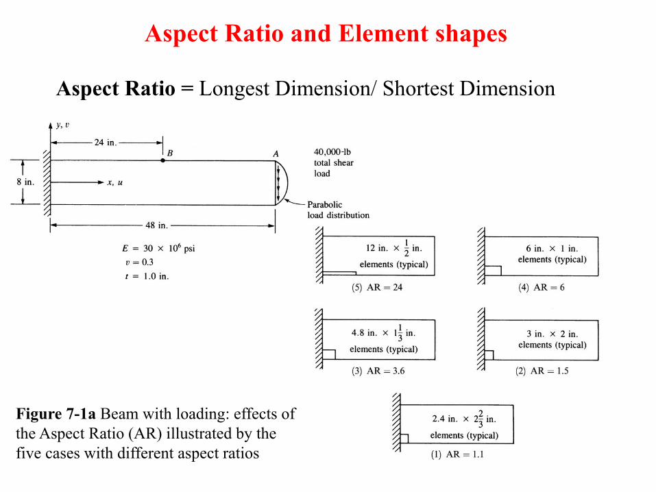
Figure 7-1a Beam with loading: effects of
the Aspect Ratio (AR) illustrated by the
five cases with different aspect ratios
Aspect Ratio = Longest Dimension/ Shortest Dimension
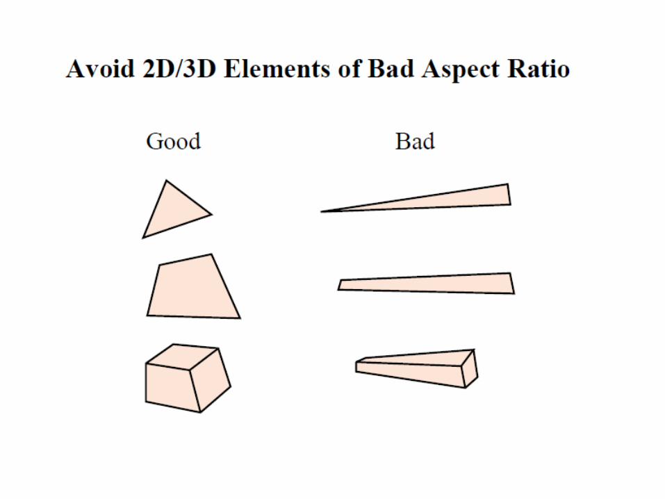
Aspect Ratio and Element shapes
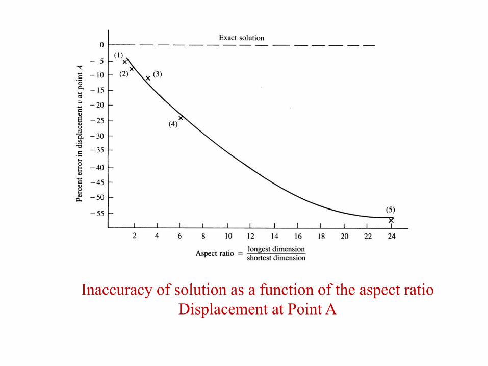
Inaccuracy of solution as a function of the aspect ratio
Displacement at Point A
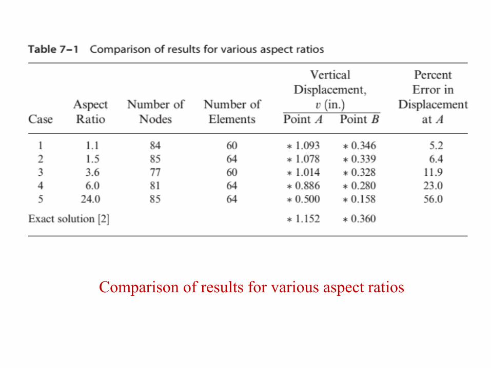
Comparison of results for various aspect ratios
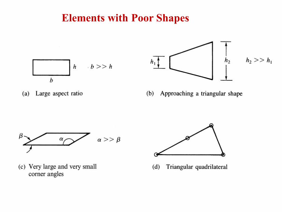
Elements with Poor Shapes
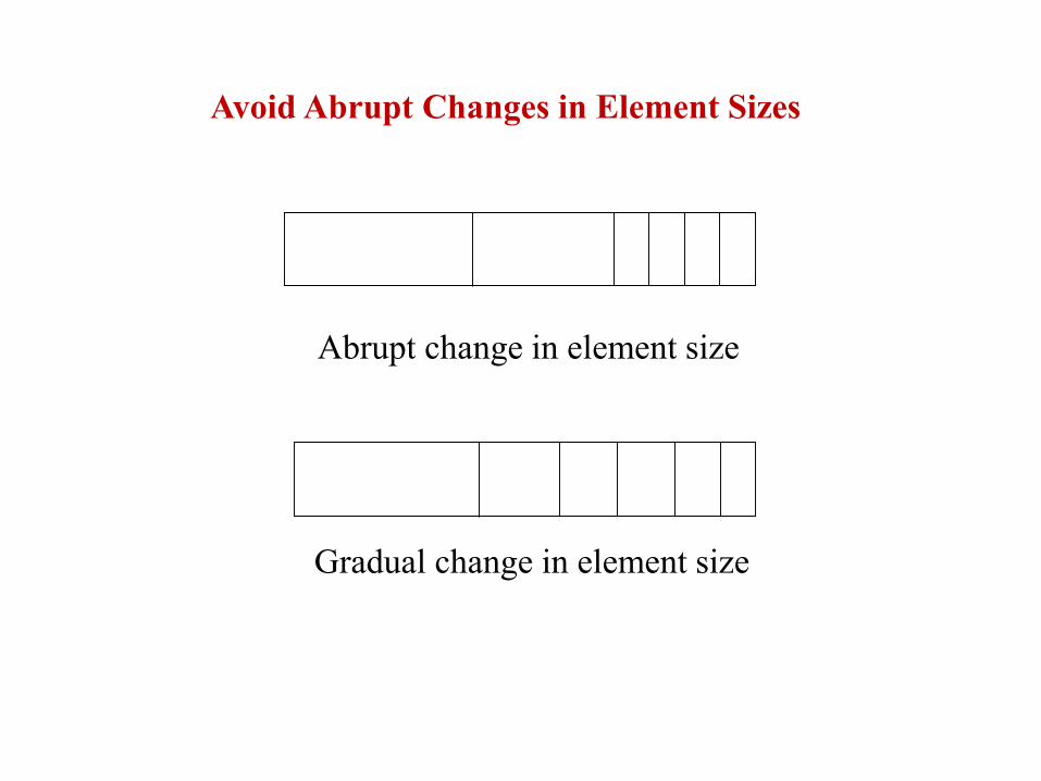
Avoid Abrupt Changes in Element Sizes
Abrupt change in element size
Gradual change in element size
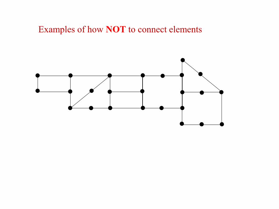
Examples of how NOT to connect elements
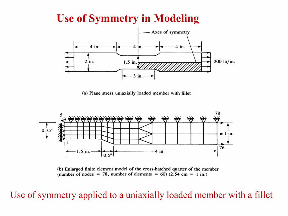
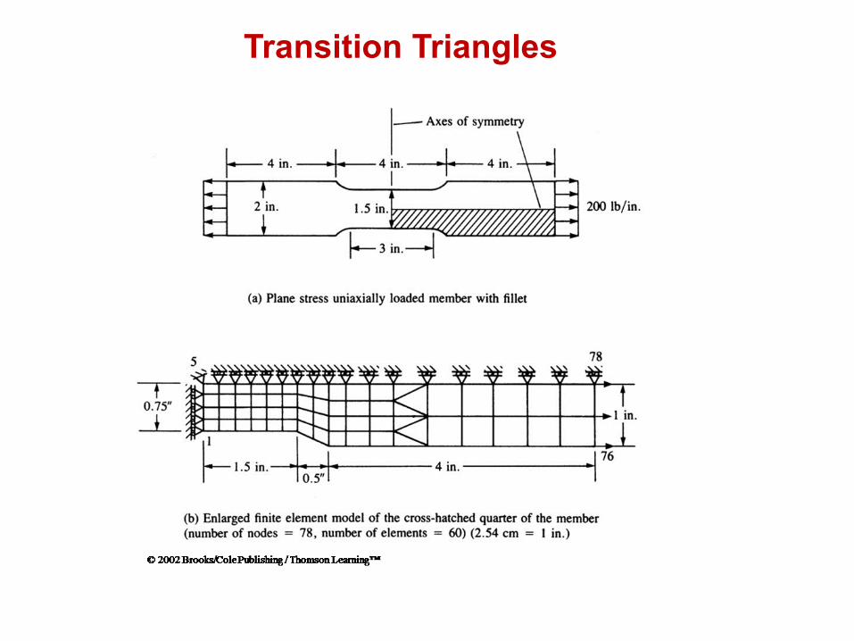
Use of symmetry applied to a uniaxially loaded member with a fillet
Use of Symmetry in Modeling
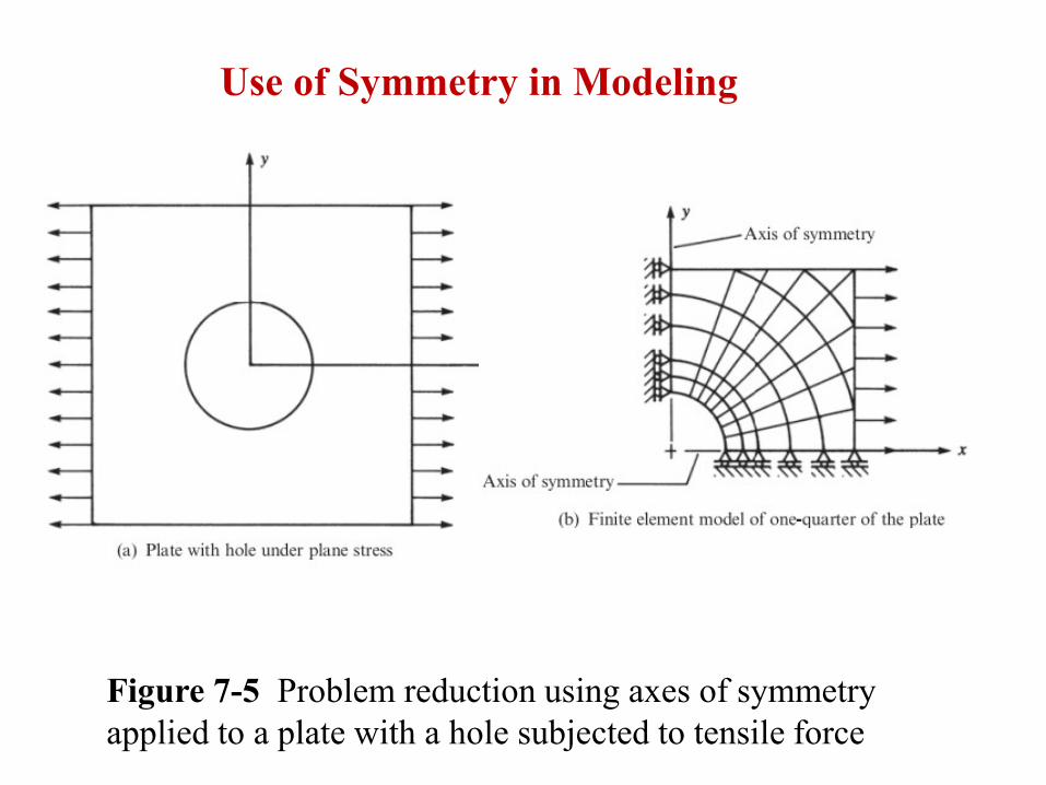
Figure 7-5 Problem reduction using axes of symmetry
applied to a plate with a hole subjected to tensile force
Use of Symmetry in Modeling
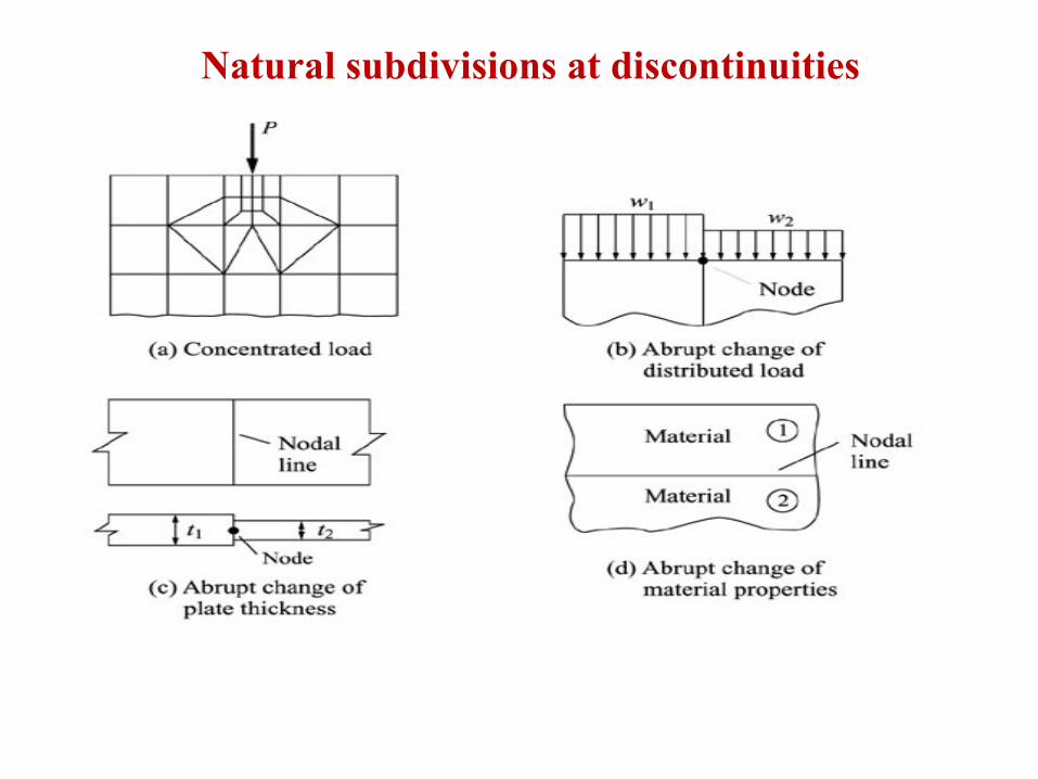
Natural subdivisions at discontinuities
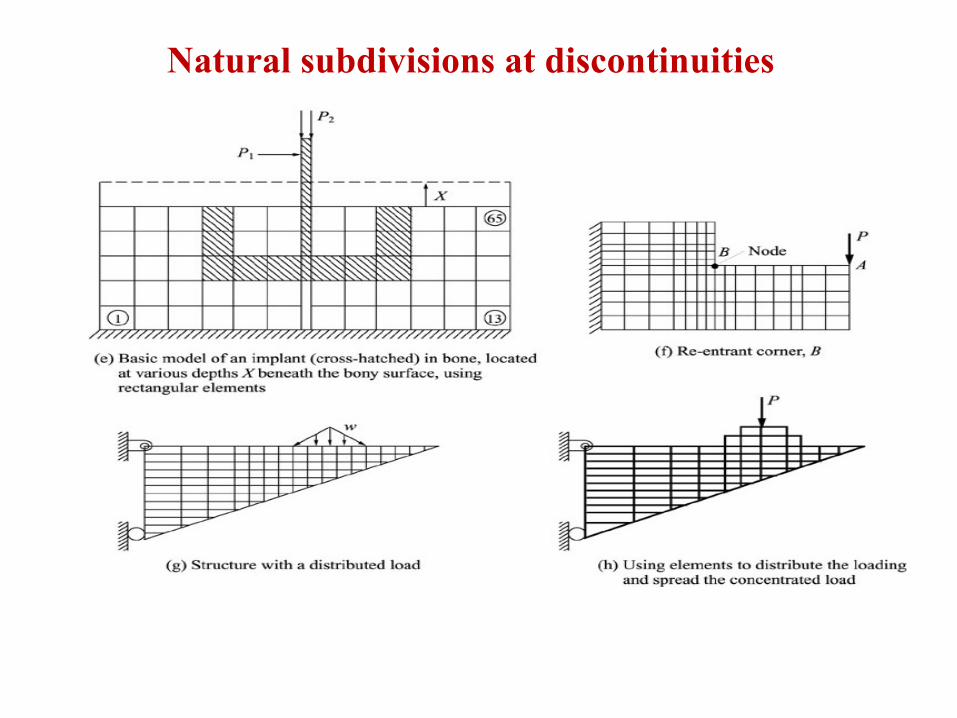
Natural subdivisions at discontinuities
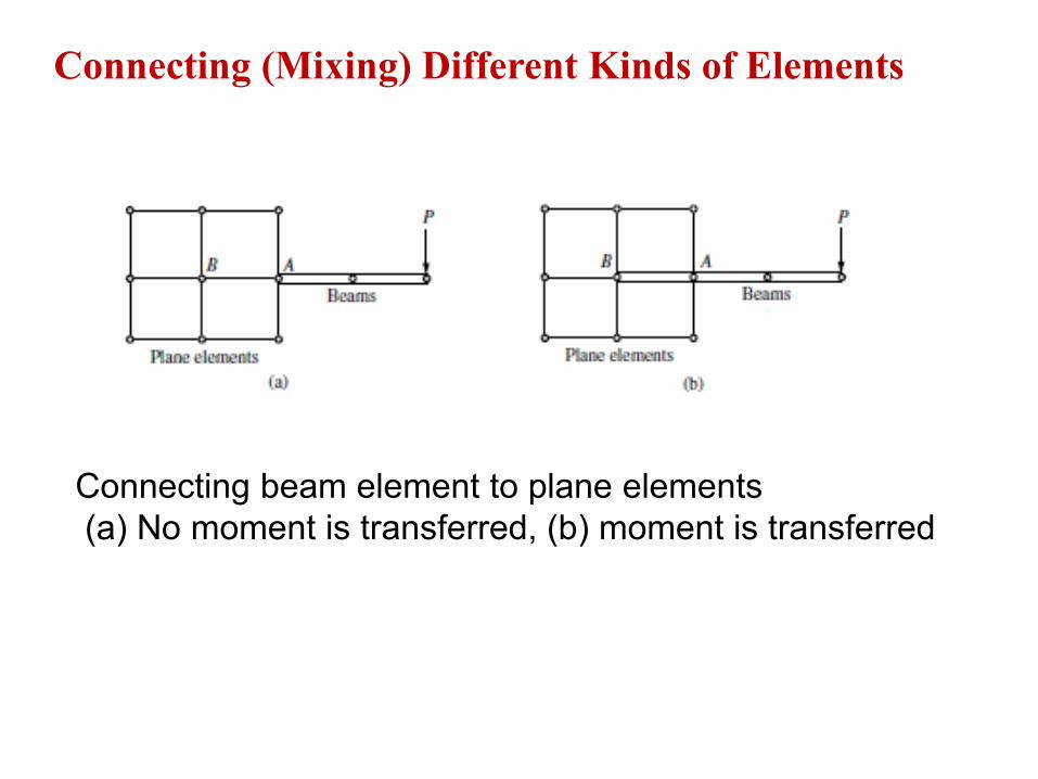
Connecting (Mixing) Different Kinds of Elements
Connecting beam element to plane elements
(a) No moment is transferred, (b) moment is transferred
Infinite Medium
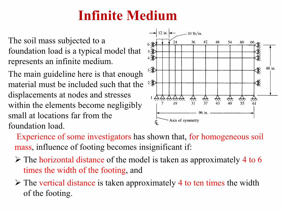
The soil mass subjected to a
foundation load is a typical model that
represents an infinite medium.
The main guideline here is that enough
material must be included such that the
displacements at nodes and stresses
within the elements become negligibly
small at locations far from the
foundation load.
Experience of some investigators has shown that, for homogeneous soil
mass, influence of footing becomes insignificant if:
The horizontal distance of the model is taken as approximately 4 to 6
times the width of the footing, and
The vertical distance is taken approximately 4 to ten times the width
of the footing.
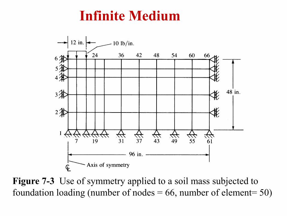
Figure 7-3 Use of symmetry applied to a soil mass subjected to
foundation loading (number of nodes = 66, number of element= 50)
Infinite Medium
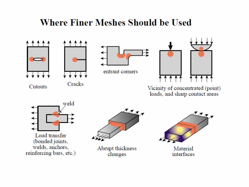
Mesh Refinement
h-refinement
p-refinement
h=element size
p=polynomial order
The discretization depends on the geometry of the structure, the loading
pattern, and the boundary conditions.
For instance, regions of stress concentration or high stress gradient due to
fillets, holes, or re-entrant corners require a finer mesh near those regions
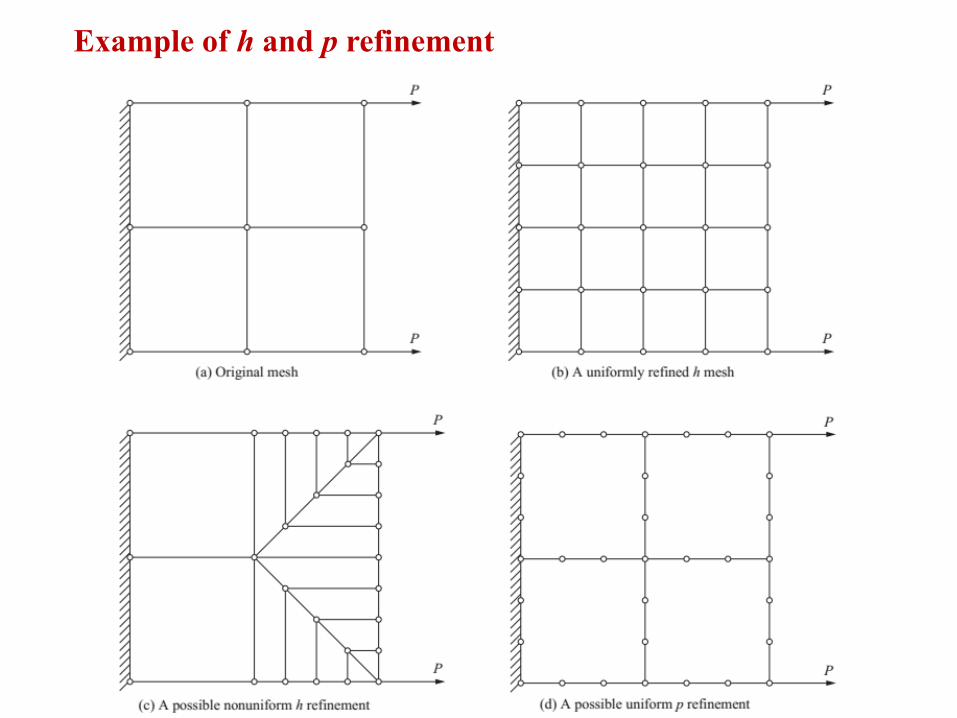
Example of h and p refinement
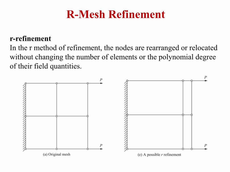
R-Mesh Refinement
r-refinement
In the r method of refinement, the nodes are rearranged or relocated
without changing the number of elements or the polynomial degree
of their field quantities.
Transition Triangles
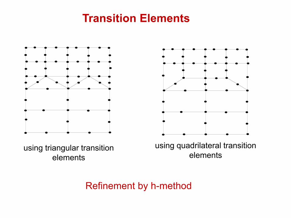
using triangular transition
elements
Transition Elements
Refinement by h-method
using quadrilateral transition
elements
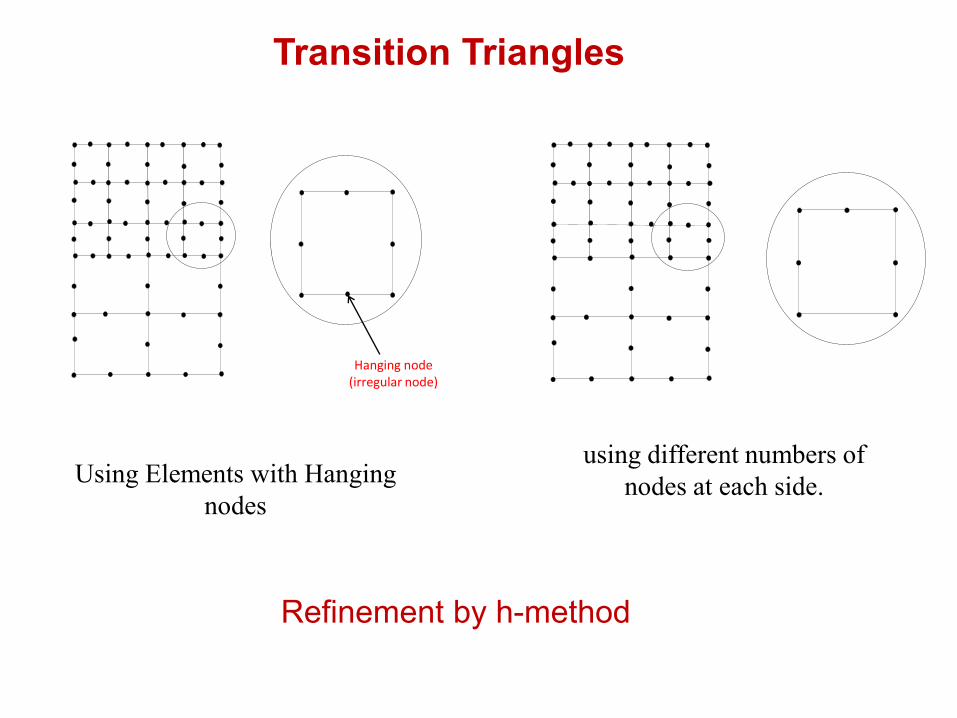
Hanging node (irregular node)
Using Elements with Hanging
nodes
using different numbers of
nodes at each side.
Transition Triangles
Refinement by h-method
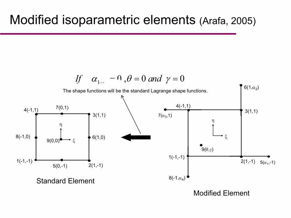
Modified isoparametric elements (Arafa, 2005)
1 4 0 , 0 0If and
The shape functions will be the standard Lagrange shape functions.
1(-1,-1)
3(1,1)4(-1,1)
2(1,-1) 5(1,-1)
8(-1,4)
6(1,2)
7(3,1)
9(,)
1(-1,-1)
3(1,1)4(-1,1)
2(1,-1)5(0,-1)
8(-1,0) 6(1,0)
7(0,1)
9(0,0)
Standard Element
Modified Element
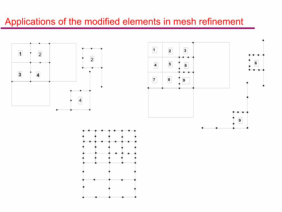
Applications of the modified elements in mesh refinement
1 2
43
2
4
1
4 5
7
2 3
8
6
9
9
6
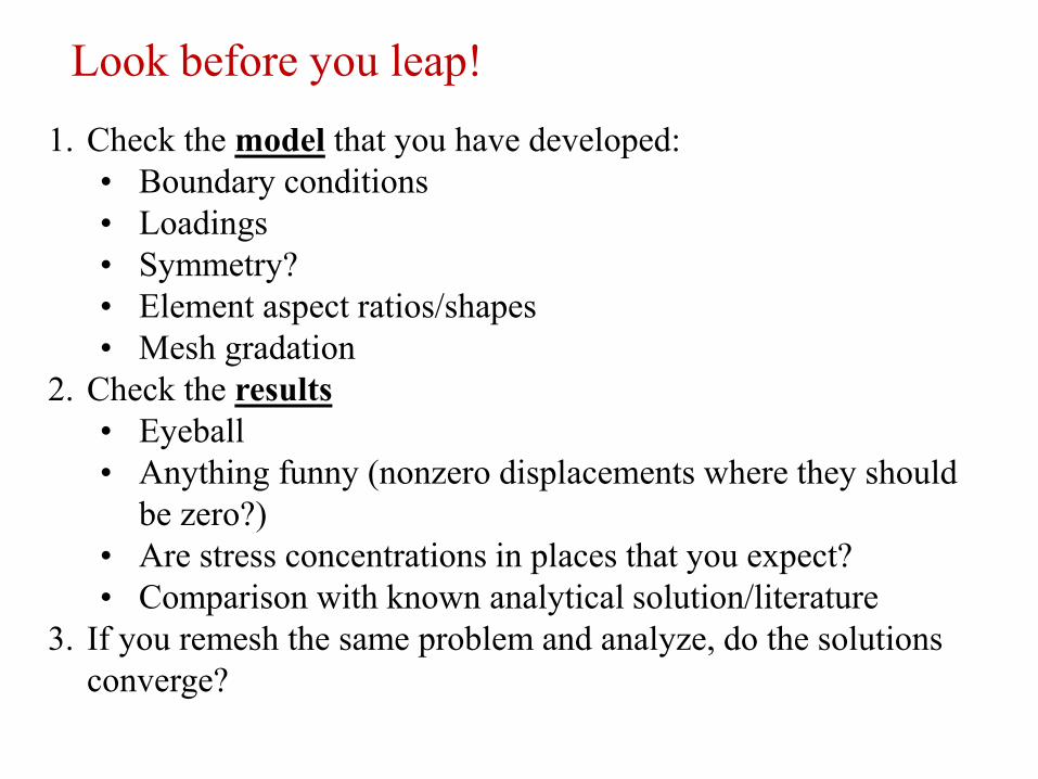
Look before you leap!
1. Check the model that you have developed:
• Boundary conditions
• Loadings
• Symmetry?
• Element aspect ratios/shapes
• Mesh gradation
2. Check the results
• Eyeball
• Anything funny (nonzero displacements where they should
be zero?)
• Are stress concentrations in places that you expect?
• Comparison with known analytical solution/literature
3. If you remesh the same problem and analyze, do the solutions
converge?
An approximate FE solution for a stress analysis problem, based
on assumed displacement fields, does not generally satisfy all the
requirements for equilibrium and compatibility that an exact
theory-of-elasticity solution satisfies.
However, remember that relatively few exact solutions exist.
Hence, the finite element method is a very practical one obtaining
reasonable, but approximate, numerical solutions.
We now describe some of the approximations generally inherent in
finite element solutions
Equilibrium and Compatibility of Finite Element
Results
1- Equilibrium of nodal forces and moments is satisfied:
This is true because the global equation F = K d is a nodal
equilibrium equation whose solution for d is such that the sums of
all forces and moments applied to each node are zero. Equilibrium
of the whole structure also satisfied because the structure reactions
are included in the global forces, and hence, in the nodal
equilibrium equations.
Equilibrium and Compatibility of Finite Element Results
2- Equilibrium within an element is not always satisfied:
For the constant-strain bar of Chapter 3 and the constant-strain
triangle of Chapter 6, element equilibrium is satisfied. The cubic
displacement function is shown to satisfy the basic beam
equilibrium differential equation in Chapter 5, and hence, to satisfy
element force and moment equilibrium. However, elements such
as the linear-strain triangle of Chapter 8 the axisymmetric element
of Chapter 9, and the rectangular element of Chapter 10 usually
only approximately satisfy the element equilibrium equations.
Equilibrium and Compatibility of Finite Element Results
3- Equilibrium is not usually satisfied between elements:
A differential element including parts of two adjacent finite
elements is usually not in equilibrium.
• For line elements, such as used for truss and frame analysis,
interelement equilibrium is satisfied as shown in examples in
Chapters 3 through 6.
• However, for two- and three-dimensional elements, interelement
equilibrium is not usually satisfied.
Equilibrium and Compatibility of Finite Element Results
4- Compatibility is satisfied within an element
Hence, individual elements do not tear apart.
5-Compatibility is satisfied at the nodes
Hence, elements remain connected at their common nodes.
Similarly, the structure remains connected to its support nodes
because boundary conditions are invoked at these nodes.
Equilibrium and Compatibility of Finite Element Results
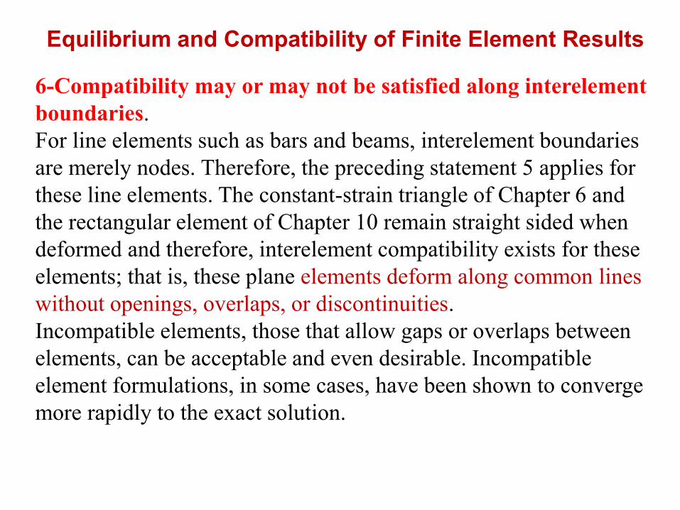
6-Compatibility may or may not be satisfied along interelement
boundaries.
For line elements such as bars and beams, interelement boundaries
are merely nodes. Therefore, the preceding statement 5 applies for
these line elements. The constant-strain triangle of Chapter 6 and
the rectangular element of Chapter 10 remain straight sided when
deformed and therefore, interelement compatibility exists for these
elements; that is, these plane elements deform along common lines
without openings, overlaps, or discontinuities.
Incompatible elements, those that allow gaps or overlaps between
elements, can be acceptable and even desirable. Incompatible
element formulations, in some cases, have been shown to converge
more rapidly to the exact solution.
Equilibrium and Compatibility of Finite Element Results
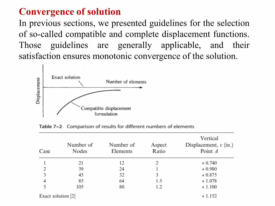
Convergence of solution
In previous sections, we presented guidelines for the selection
of so-called compatible and complete displacement functions.
Those guidelines are generally applicable, and their
satisfaction ensures monotonic convergence of the solution.
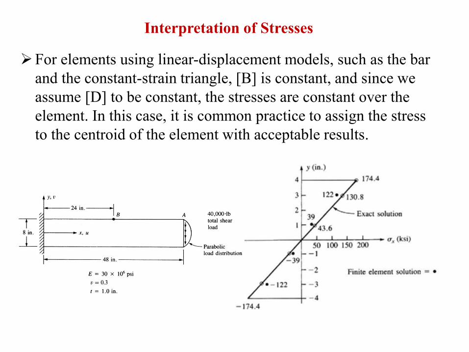
Interpretation of Stresses
For elements using linear-displacement models, such as the bar
and the constant-strain triangle, [B] is constant, and since we
assume [D] to be constant, the stresses are constant over the
element. In this case, it is common practice to assign the stress
to the centroid of the element with acceptable results.
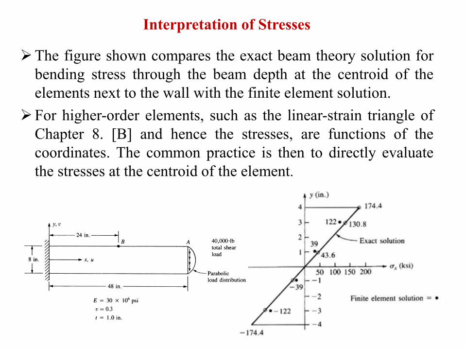
Interpretation of Stresses
The figure shown compares the exact beam theory solution for
bending stress through the beam depth at the centroid of the
elements next to the wall with the finite element solution.
For higher-order elements, such as the linear-strain triangle of
Chapter 8. [B] and hence the stresses, are functions of the
coordinates. The common practice is then to directly evaluate
the stresses at the centroid of the element.
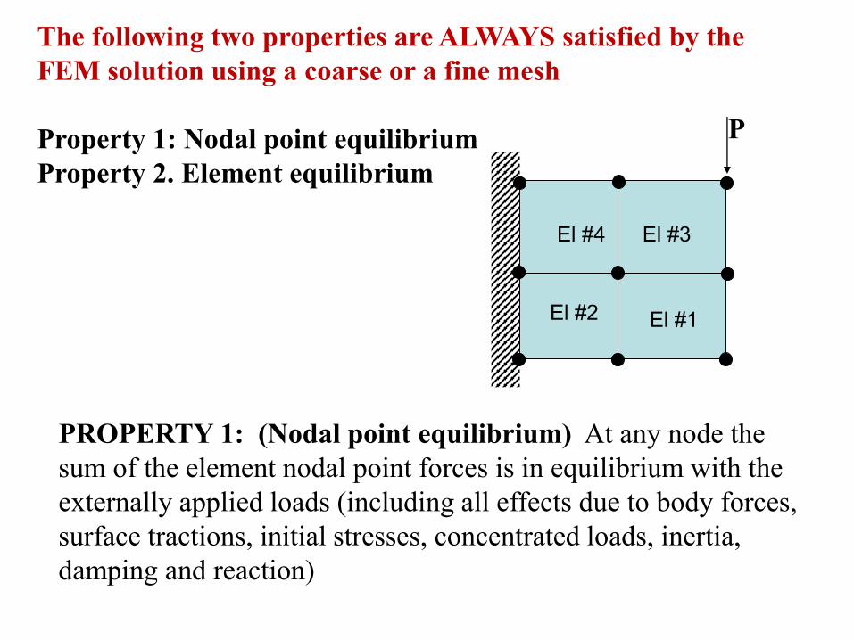
The following two properties are ALWAYS satisfied by the
FEM solution using a coarse or a fine mesh
Property 1: Nodal point equilibrium
Property 2. Element equilibrium
El #4 El #3
El #1El #2
P
PROPERTY 1: (Nodal point equilibrium) At any node the
sum of the element nodal point forces is in equilibrium with the
externally applied loads (including all effects due to body forces,
surface tractions, initial stresses, concentrated loads, inertia,
damping and reaction)
El #4 El #3
El #1El #2
P
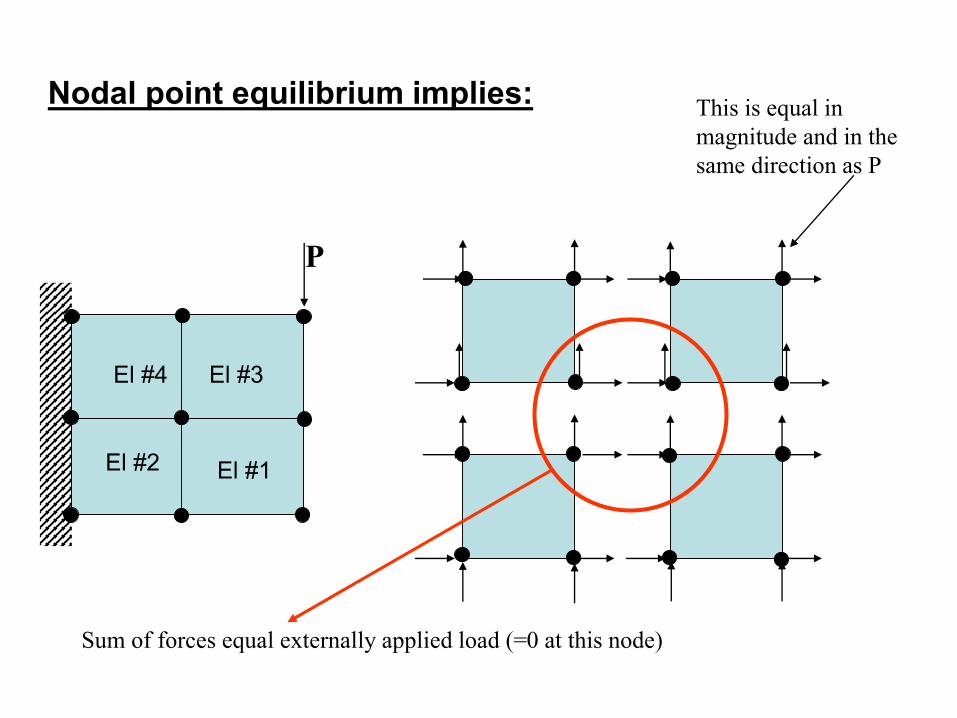
This is equal in
magnitude and in the
same direction as P
Sum of forces equal externally applied load (=0 at this node)
Nodal point equilibrium implies:
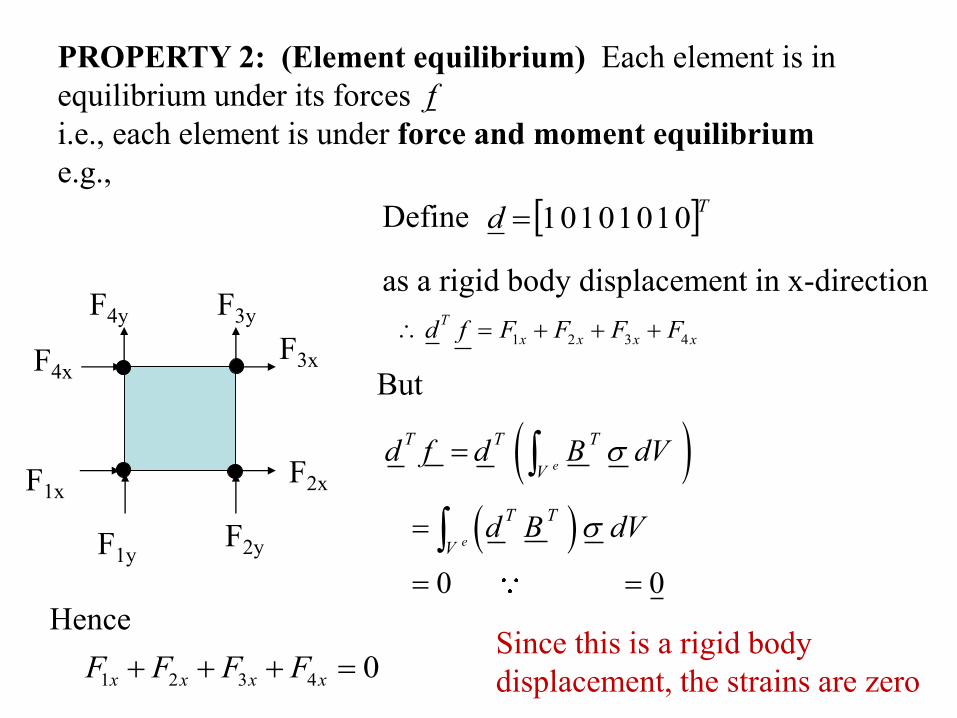
PROPERTY 2: (Element equilibrium) Each element is in
equilibrium under its forces f
i.e., each element is under force and moment equilibrium
e.g.,
F3x
F2xF1x
F4x
F1yF2y
F3yF4y
Define Td 01010101
0 0
e
e
T T T
V
T T
V
d f d B dV
d B dV
B d
1 2 3 4
T
x x x xd f F F F F
But
Since this is a rigid body
displacement, the strains are zero
Hence
1 2 3 4 0x x x xF F F F
as a rigid body displacement in x-direction
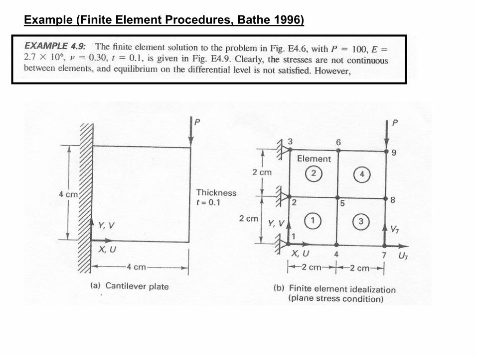
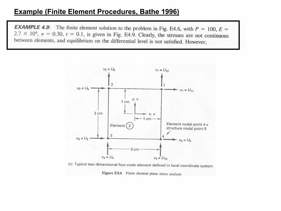
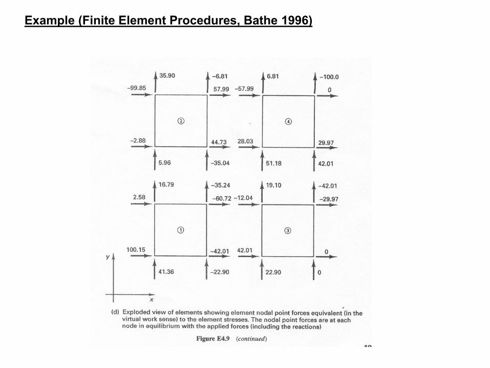
Example (Finite Element Procedures, Bathe 1996)
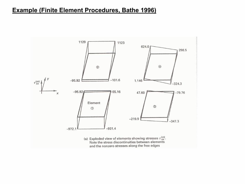
Example (Finite Element Procedures, Bathe 1996)
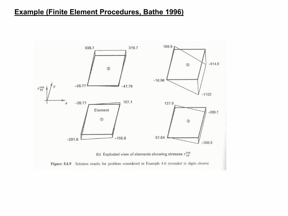
Example (Finite Element Procedures, Bathe 1996)
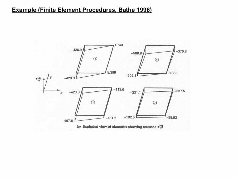
Example (Finite Element Procedures, Bathe 1996)
Example (Finite Element Procedures, Bathe 1996)
Example (Finite Element Procedures, Bathe 1996)
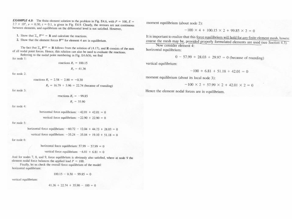
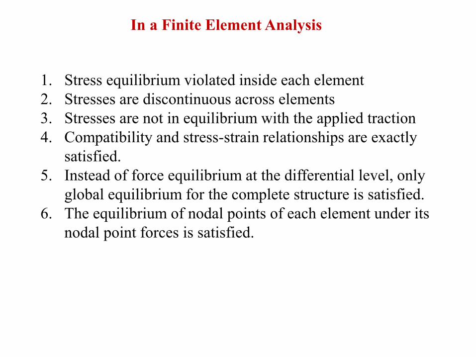
1. Stress equilibrium violated inside each element
2. Stresses are discontinuous across elements
3. Stresses are not in equilibrium with the applied traction
4. Compatibility and stress-strain relationships are exactly
satisfied.
5. Instead of force equilibrium at the differential level, only
global equilibrium for the complete structure is satisfied.
6. The equilibrium of nodal points of each element under its
nodal point forces is satisfied.
In a Finite Element Analysis
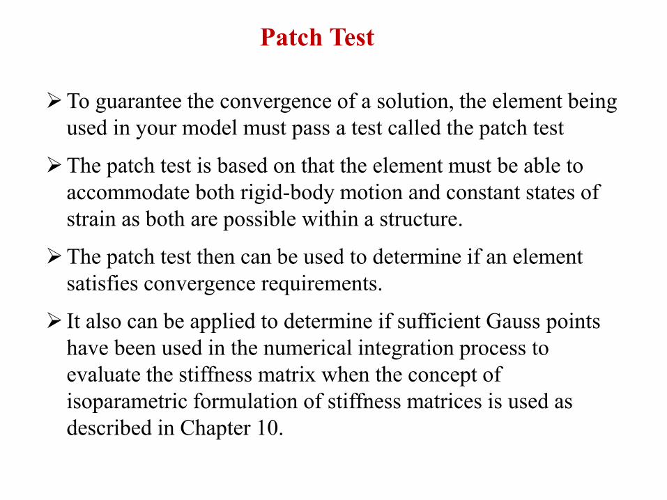
To guarantee the convergence of a solution, the element being
used in your model must pass a test called the patch test
The patch test is based on that the element must be able to
accommodate both rigid-body motion and constant states of
strain as both are possible within a structure.
The patch test then can be used to determine if an element
satisfies convergence requirements.
It also can be applied to determine if sufficient Gauss points
have been used in the numerical integration process to
evaluate the stiffness matrix when the concept of
isoparametric formulation of stiffness matrices is used as
described in Chapter 10.
Patch Test
The patch test is performed by considering a simple finite
element model composed of four irregular shaped elements of
the same material with at least one node inside of the patch
(called the patch node),
The elements should be irregular, as some regular elements
(such as rectangular) may pass the test whereas irregular ones
will not.
The elements may be all triangles or quadrilaterals or a mix of
both. The boundary can be a rectangle though
Patch Test
Step 1 Assume a uniform stress state of x =1 or some
convenient constant value is applied along the right side of the
patch. Replace this stress with its work-equivalent nodal load.
Step 2 Internal node 5 is not loaded.
Step 3 The patch has just enough supports to prevent rigid-
body motion. Step 4 The finite element direct stiffness method
is again used to obtain the
displacements and element stresses. The uniform stress sx ¼ 1
should be
Patch Test
The ‘‘displacement’’ Patch Test
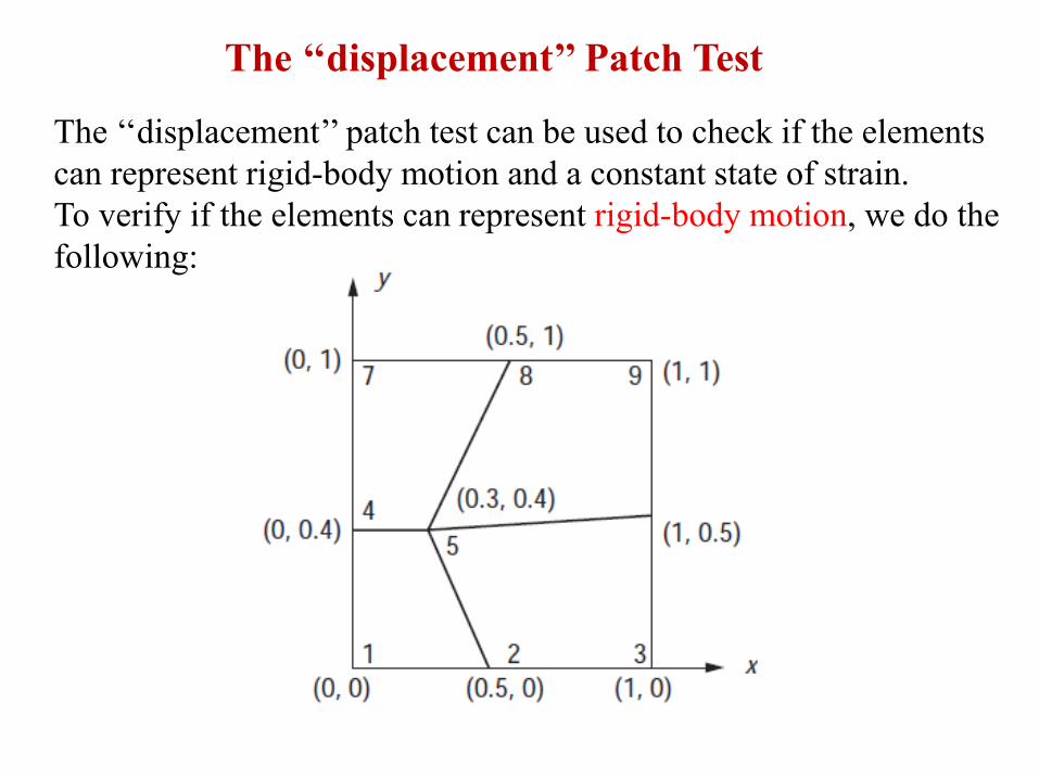
The ‘‘displacement’’ patch test can be used to check if the elements
can represent rigid-body motion and a constant state of strain.
To verify if the elements can represent rigid-body motion, we do the
following:
The ‘‘displacement’’ Patch Test
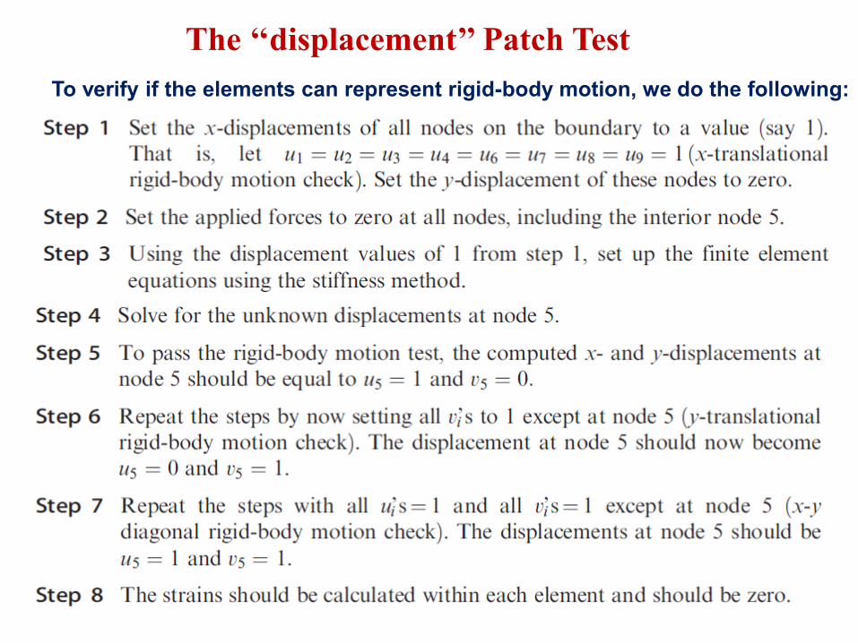
To verify if the elements can represent rigid-body motion, we do the following:
The ‘‘displacement’’ Patch Test
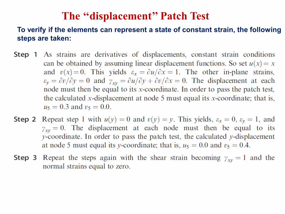
To verify if the elements can represent a state of constant strain, the following
steps are taken:
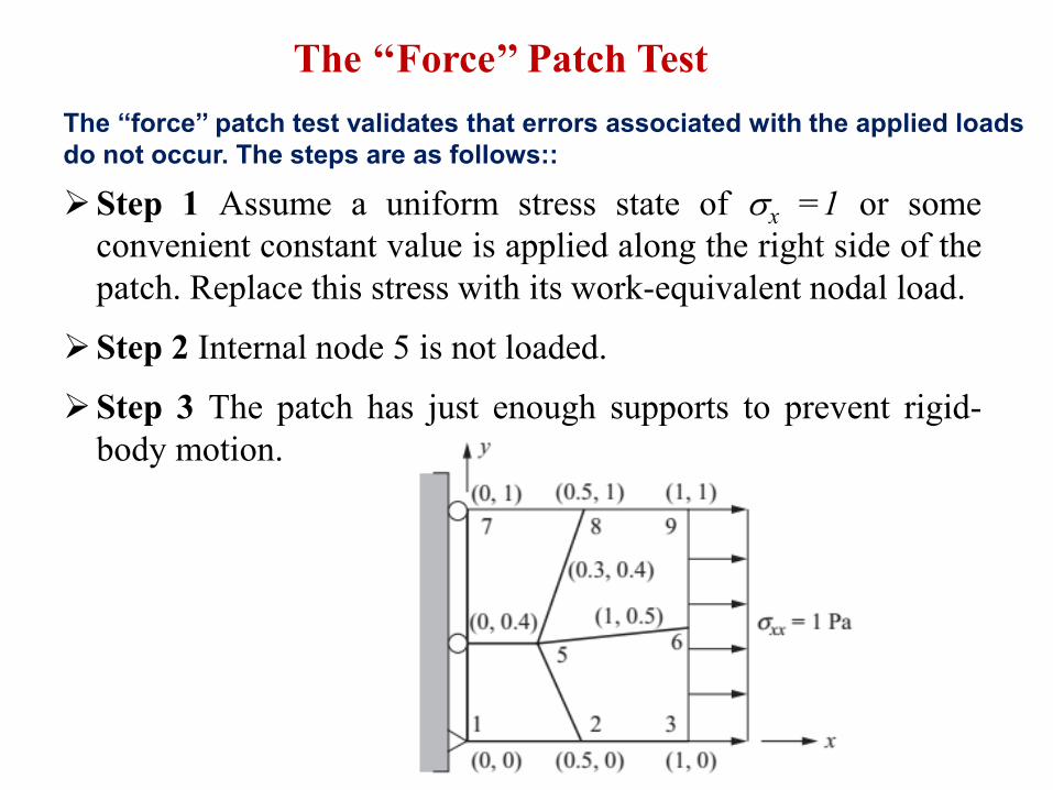
The ‘‘Force’’ Patch Test
The ‘‘force’’ patch test validates that errors associated with the applied loads
do not occur. The steps are as follows::
Step 1 Assume a uniform stress state of x =1 or some
convenient constant value is applied along the right side of the
patch. Replace this stress with its work-equivalent nodal load.
Step 2 Internal node 5 is not loaded.
Step 3 The patch has just enough supports to prevent rigid-
body motion.
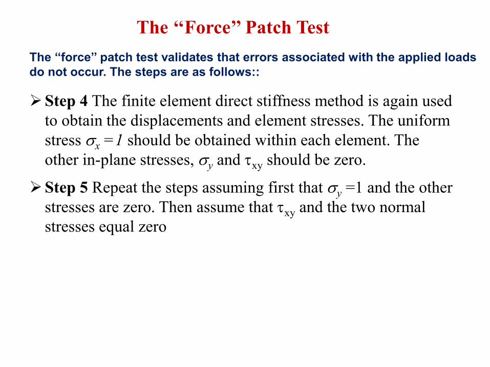
The ‘‘Force’’ Patch Test
The ‘‘force’’ patch test validates that errors associated with the applied loads
do not occur. The steps are as follows::
Step 4 The finite element direct stiffness method is again used
to obtain the displacements and element stresses. The uniform
stress x =1 should be obtained within each element. The
other in-plane stresses, y and xy should be zero.
Step 5 Repeat the steps assuming first that y =1 and the other
stresses are zero. Then assume that xy and the two normal
stresses equal zero
The Patch Test
An element that passes the patch test is capable of meeting the following
requirements:
a) Predicting rigid-body motion without strain when this state exists.
b) Predicting states of constant strain if they occur.
c) Compatibility with adjacent elements when a state of constant strain
exists in adjacent elements.
When these requirements are met, it is sufficient to guarantee that a mesh
of these elements will yield convergence to the solution as the mesh is
continually refined.
The patch test is a standard test for developers of new elements.
Whether the element has the necessary convergence properties. But the test
does not indicate how well an element works in other applications. An
element passing the patch test may still yield poor accuracy in a coarse
mesh or show slow convergence as the mesh is refined.