Mapping Sectoral Patterns of Technological

Accumulation into the Geography of Corporate

Locations. A Simple Model and Some Promising

Evidence.

Giulio Bottazzi∗ Giorgio Fagiolo† Giovanni Dosi‡

February 10, 2003

Abstract

Economies of agglomeration are central to the understanding of the emergence ofindustrial clustering. However, existing models that incorporate such agglomera-tion economies have been largely neglecting the vast amount of empirical evidenceon inter-sectoral differences in the patterns of industrial concentration. In this pa-per, we propose a baseline model of firm location in presence of dynamic increasingreturns. The model is able to deliver testable implications about the long-run dis-tribution of the size of spatial clusters which we test against data on geographicallocation of Italian firms belonging to different sectors. We show that accordance oftheoretical predictions with data is quite high. Moreover, we find statistically sig-nificant differences in the strength of economies of agglomeration, not only acrossgeographical locations but also across industrial sectors. We argue that geograph-ical clustering is highly affected by intersectoral differences in innovation patternsand learning regimes that map into different drivers of sector- and location-specificdynamic increasing returns to agglomeration.

Keywords: Industrial Clustering, Economies of Agglomeration, Firm LocationalChoice, Dynamics.

JEL Classification: F12, R10.∗Sant’Anna School of Advanced Studies, Pisa, Italy. Email: bottazzi@sssup.it†Corresponding Author. Sant’Anna School of Advanced Studies, Laboratory of Economics and Man-

agement (LEM), Piazza Martiri della Libertà, 33, I-56127 PISA (Italy). Email: fagiolo@sssup.it. Tel:+39-050-883341. Fax: +39-050-883344.

‡Sant’Anna School of Advanced Studies, Pisa, Italy. Email: gdosi@sssup.it

1

1 Introduction

Over the last two decades, there has been a widespread resurgence of studies sharing the

notion that “space matters in economic activity”. In particular, much effort has been

devoted to a theoretical exploration of the mechanisms underlying the process of industrial

clustering both within and across countries.

Patterns of spatial concentration of firms have often been interpreted in a comparative

advantage framework as the outcome of a static, well-defined, trade-off between agglomera-

tion and dispersion forces1. In this view, spatial locations display ex-ante, well identifiable,

differences in initial endowments, transport costs and market interactions which uniquely

determine the observed industrial concentration as a predictable equilibrium outcome.

However, the vast amount of empirical and appreciative studies about firm locational

patterns in the U.S., Asia and Europe, seems to suggest that industries are more highly

clustered than any standard theory of comparative advantage might predict (cf. Krugman

(1991) and Fujita, Krugman & Venables (1999)).

Many interpretations have consequently assumed that the primary engine of concentra-

tion lies instead in some form of economies of agglomeration (i.e. positive market external-

ities). Long-run concentration patterns would therefore arise because of a self-reinforcing

process in which the decision of a firm to locate in a given area induces a net increase in

profits enjoyed by firms deciding to follow her thereafter. As a result, clustering processes

might display multiple equilibria and path-dependence. Historical accidents could then

have long-run cumulative consequences, possibly leading to agglomeration patterns that

would not have been selected on the basis of initial conditions only.

Within a such an expanding literature, distinct families of models subscribe to quite

different assumptions, on both system-level drivers of agglomeration and microeconomic

behaviors. On the one hand, the ‘New Economic Geography’ (NEG) perspective (see Fu-

1This intuition, pioneered by Von Thünen (1826) and further developed by Christaller (1933) andLösch (1940), also informs studies in Isard (1956) and Henderson (1974) on urban systems. For morerecent studies, see Papageorgiou & Smith (1983), Fujita (1988) and Fujita (1989).

2

jita, Krugman & Venables (1999)) primarily focuses on locational choices undertaken by

fully informed ‘rational’ firms who live within static environments and interact in monopo-

listically competitive markets. On the other hand, a second class of formalizations is based

on quite distinct assumptions, including sequential, irreversible, decisions made by adap-

tive firms who interact in explicitly dynamic environments (cf. Arthur (1994) and Rauch

(1993)).

Notwithstanding their respective merits and weaknesses (cf. Martin (1999) for a criti-

cal overview), it is rather remarkable that both approaches largely share the neglect for a

parallel, massive, literature from innovation studies concerning sector-specific processes of

technological learning, bearing obvious effects upon the locational stickiness of productive

knowledge; the different nature and importance of technological externalities and spillovers;

the abilities of incumbents to internalize and ‘carry within themselves’ knowledge comple-

mentarities. In brief, one still witnesses a dramatic lack of dialogue between economic

geography and ‘spatial’ economics, on the one hand, and the economics of technological

change, on the other.

This work is meant as a preliminary contribution to fill this large gap. We explore the

basic drivers of spatial agglomeration processes of economic activities and their specificities,

both across industries and across spatial locations. More specifically, we ask the following

questions: How can one explain the huge, empirically observed, differences in agglomeration

patterns across industrial sectors? Are there systematic agglomeration drivers that are

entirely sector-specific and operate besides local agglomeration forces (possibly generated

by some widespread form of dynamic increasing returns or spatial externalities) inducing

concentration independent of technological and learning characteristics of each firm?

In order to address these issues, we propose a simple stochastic model of industrial clus-

tering in which myopic firms make locational choices in presence of dynamic agglomeration

economies. The latter stem from both standard comparative advantage arguments (making

some locations inherently more attractive than others) and dynamic increasing returns in

locating close to other firms. In turn, dynamic increasing returns may be characterized

3

by both location-specific and technology-specific drivers. Therefore, heterogeneous concen-

tration patterns among geographical sites and industrial sectors are likely to arise. The

model yields empirically testable predictions on the equilibrium distribution of the size

of spatial clusters and on the diverse relevance of agglomeration forces across industrial

sectors. We compare the predictions of the model with some evidence on the geographical

distribution of Italian firms across a set of industries which might be considered archetypes

of distinct regimes of technological learning (see Pavitt (1984), Dosi (1988), Malerba &

Orsenigo (1996) and Marsili (2001)). The evidence strongly supports the view that in-

tersectoral differences in economies of agglomeration might be (at least partly) explained

by differences in innovation patterns and learning regimes displayed by firms belonging to

diverse industrial sectors.

The rest of the paper is organized as follows. In Section 2 we briefly discuss the

state-of-the-art on both theoretical and empirical studies of spatial clustering of economic

activities. Section 3 describes the model. In Section 4 we present testing procedures and

econometric results with reference to some benchmark industries (i.e. leather products,

transport equipment, electronics, financial intermediation services). Finally, in Section 5,

we suggest some extensions of the basic model and directions for future work.

2 Economies of Agglomeration and Industrial Con-

centration: Theory vs. Empirical Evidence

In a nutshell, one might identify four main questions that scholars concerned about the

‘spatial dimension’ of economic interactions have been all trying to address, albeit from

different perspectives, for more than a century, namely: (i) Could one neatly identify

agglomeration (centripetal) and dispersion (centrifugal) forces lying at the heart of the

processes generating sustained spatial concentration (and possibly its destabilization)? (ii)

Why and when could one observe persistent spatial patterns that cannot be explained

4

by resorting to pre-existing heterogeneity in agents and locations (i.e. by some kind of

“comparative advantage theory” alone)? (iii) What is the role of mere “chance” in the

observed spatial concentration of economic activities? And: (iv) How and when emerging

spatial structures of production and innovation tend to become self-sustained over time?

(And, conversely, what make them wither away?)

As well known, Von Thünen (1826) and Marshall (1920) have been among the pioneers

in the investigation of economic forces driving geographical differentiation and agglomer-

ation. For instance, Von Thunen’s simple analysis of land use - by stressing the impor-

tance of space constraints in decentralized economies - began to uncover the relationships

between micro decisions and macro geographical outcomes. Even more importantly, Mar-

shall’s discussion of the ‘localization externalities triad’2 became a cornerstone in the theory

of economic agglomeration. From then on, however, diverse trajectories of theoretically-

grounded exploration emerged.

A first family of models has been hinging upon the basic idea that many different

spatial agglomeration patterns (from concentration of economic activities in few locations

to hierarchical structures) can be explained as the solution of a static, well-defined, trade-

off between identifiable agglomeration and dispersion forces. This intuition, rooted once

again in Von Thunen’s work, has become the core of the analyses provided by ‘central-

place’ theory developed by Christaller (1933) and Lösch (1940), of ‘regional science’ models

building on Isard (1956) and of the treatment of urban systems by Henderson (1974).

More recently, it has inspired models with non-market externalities such as Papageorgiou

& Smith (1983), Fujita (1988) and Fujita (1989).

A second class of models that has become prominent in the last few years, known

under the heading of ‘New Economic Geography’ (NEG)3, acknowledges instead some form

of increasing returns (or indivisibilities) as both the incentive triggering agglomeration

2That is: (i) backward/forward linkages associated to the trade-off between market-size and market-access; (ii) informational spillovers and (iii) advantages of thick markets for specialized local providers ofinputs.

3See Fujita, Krugman & Venables (1999) and references therein.

5

and the force able to sustain concentration (once the latter has emerged). One of the

achievements of this stream of research has been to provide a treatment of some form of

increasing returns cum monopolistic competition in a static equilibrium framework with

fully rational agents. By bridging monopolistic competition models (cf. Dixit & Stiglitz

(1977)) and Samuelson “iceberg-like” trade costs (cf. Samuelson (1952)), such models

have been able to account for agglomeration patterns and inter-locational specialization by

positing a self-reinforcement process - stemming from some form of market externality -

which finds its counterpart in dispersion forces caused either by agglomeration itself or by

the immobility of some factors (e.g. labor)4.

Third, building on inspiring works by Brian W. Arthur and Paul David, a few scholars

have been attempting to analyze the nature of economies/diseconomies of agglomeration

in explicitly dynamic frameworks where persistent spatio-temporal patterns emerge out of

the very sequence of interactions among heterogeneous economic agents. By acknowledging

the history- (or path-) dependent nature of the observed uneven spatial distribution of

economic activities, the basic argument stresses the importance of dynamic increasing

returns implied by some form of agglomeration economies/diseconomies (cf. Arthur (1994,

Chs. 4 and 6)) and/or local network externalities (cf. David, Foray & Dalle (1998) and

Cowan & Cowan (1998)). Notwithstanding their high level of abstraction, these models

are able to account for a rather wide array of spatial outcomes and to shed some light on

the ability of economies/diseconomies of agglomeration to shape long-run concentration

patterns. Together, they highlight how early, small, mainly non-predictable, events might

dynamically interact with more systematic forces in conveying persistent spatial structures.

Conversely, from a more inductive perspective, many scholars have been offering a

wealth of qualitative analyses, building on several pieces of evidence on urban/regional

development and industrial agglomeration phenomena5. Furthermore, a long stream of

4Extensions of the baseline NEG model range from urban systems and city formation (Fujita, Krugman& Mori (1999)), industrial specialization in an array of imperfectly competitive sectors (Venables (1998))and growth (Fujita, Krugman & Venables (1999, Ch.4)).

5We refer here to the ‘economic geography’ literature (see Lee & Willis (1997) for a survey and thereferences in Martin (1999)), which includes studies on industrial districts, cf. Antonelli (1990), Sforzi

6

literature on multinational investment - from the pioneering works by Vernon (1966), all

the way to the recent contributions by Cantwell and colleagues (cf. e.g. Cantwell (1989) and

Cantwell & Iammarino (1998)) - are rich of insights on the interaction between technologies,

corporate strategies and locational features.

A survey of the evidence discussed in this enormous literature is well beyond the scope

of this paper (cf. Bottazzi, Dosi & Fagiolo (2002) for a more detailed discussion and some

taxonomic attempts). Here, let us just mention two sets of empirical regularities which are

of particular interest in what follows.

First, agglomeration phenomena typically yield quite different ‘types’ of local structures.

Examples range from: (i) ‘horizontally diversified agglomerations’ (whereby activities pre-

viously vertically integrated within individual firms undergo a sort of ‘Smithian’ process of

division of labor cum branching out of different firms); to: (ii) ‘hierarchical spatially local-

ized clusters’ (which generally involve an “oligopolistic core” together with subcontracting

networks); and: (iii) ‘Silicon Valley’ districts (where agglomeration phenomena are driven

by knowledge complementarities - at least partly fueled by ‘exogenous science’).

A high sectoral variability in agglomeration structures and in the nature of agglomer-

ation drivers clearly hints at the existence of large underlying sectoral and geographical

specificities permeating agglomeration processes. In this perspective, a second, related, set

of robust empirical evidence concerns the huge intersectoral differences in the revealed spa-

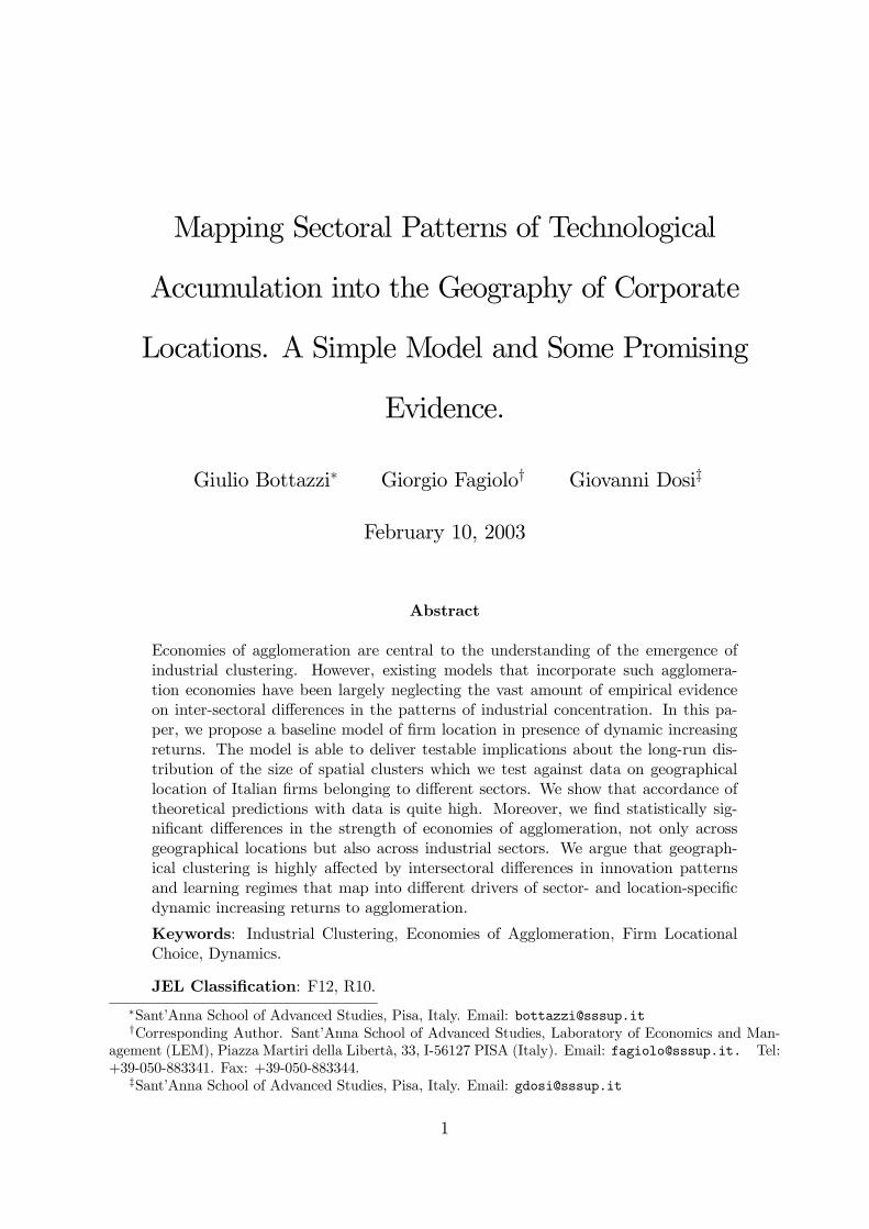
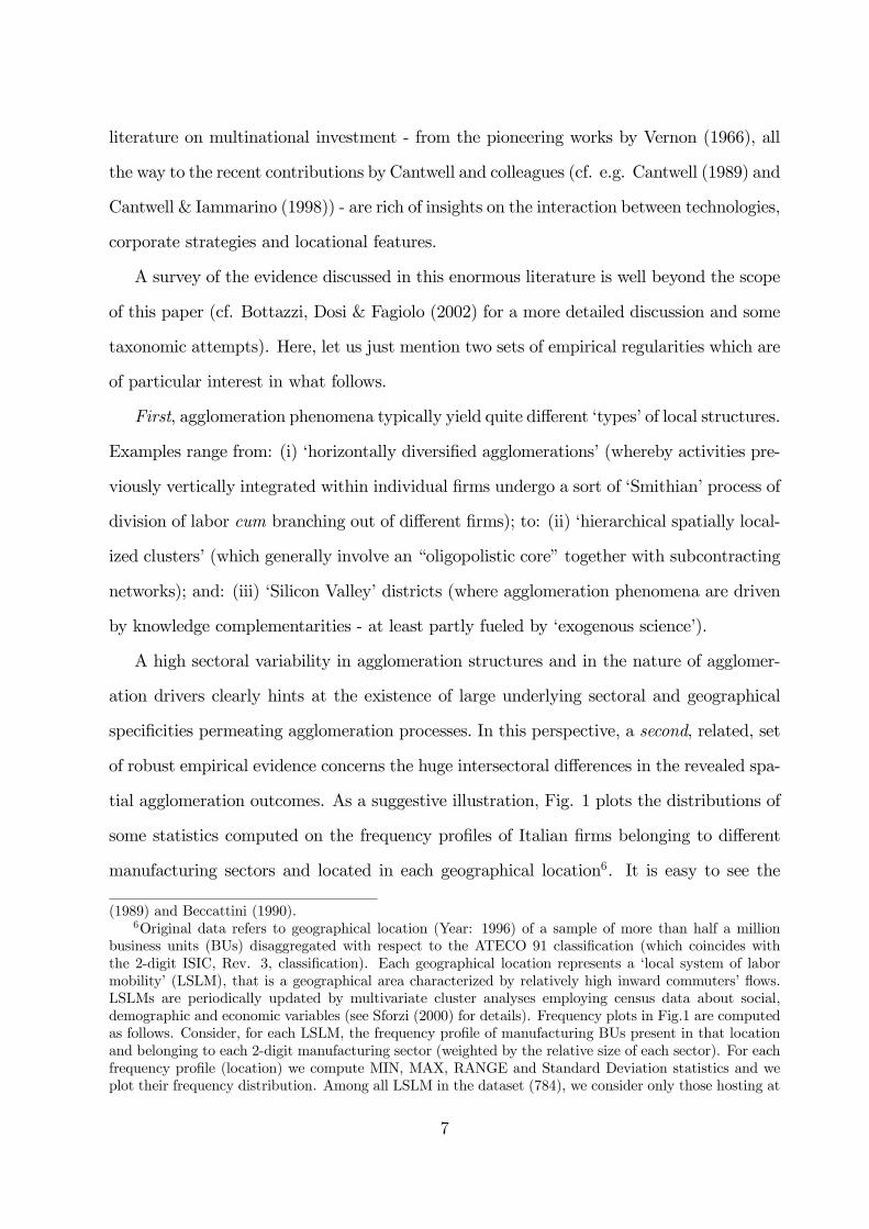
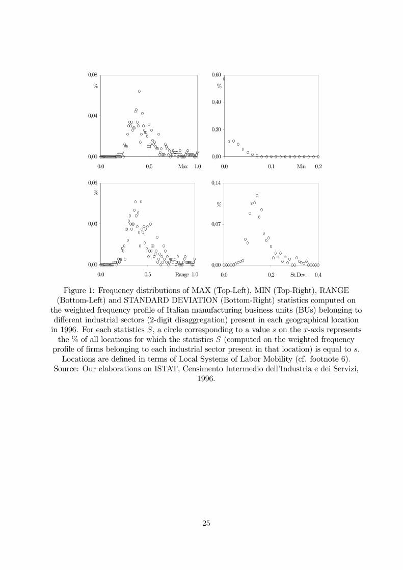
tial agglomeration outcomes. As a suggestive illustration, Fig. 1 plots the distributions of

some statistics computed on the frequency profiles of Italian firms belonging to different

manufacturing sectors and located in each geographical location6. It is easy to see the

(1989) and Beccattini (1990).6Original data refers to geographical location (Year: 1996) of a sample of more than half a million

business units (BUs) disaggregated with respect to the ATECO 91 classification (which coincides withthe 2-digit ISIC, Rev. 3, classification). Each geographical location represents a ‘local system of labormobility’ (LSLM), that is a geographical area characterized by relatively high inward commuters’ flows.LSLMs are periodically updated by multivariate cluster analyses employing census data about social,demographic and economic variables (see Sforzi (2000) for details). Frequency plots in Fig.1 are computedas follows. Consider, for each LSLM, the frequency profile of manufacturing BUs present in that locationand belonging to each 2-digit manufacturing sector (weighted by the relative size of each sector). For eachfrequency profile (location) we compute MIN, MAX, RANGE and Standard Deviation statistics and weplot their frequency distribution. Among all LSLM in the dataset (784), we consider only those hosting at

7

high variability in the distribution of manufacturing sectors across geographical sites. For

instance, there exists a high number of locations where firms belonging to almost all sectors

are equally represented. On the contrary, for a quite large frequency of sites, agglomeration

occurs only for firms belonging to a small number of sectors (in some cases 1 or 2). More

generally, in more than 50% of locations, a quite large fraction of sectors are not even

represented.

Taken together, these two pieces of evidence suggest a picture where different drivers

of agglomeration, which might be economy-wide, location-specific and/or sector-specific,

interact over time (at possibly different time- and space-scales) leading to patterns of

concentration exhibiting high variability both across locations and across industries. In

turn, different types of drivers of agglomeration seem to be often nested in the nature of

sector-specific patterns of knowledge accumulation.

Indeed, the main conjecture that we want to explore in this paper is that cross-sectoral

differences in agglomeration forces ought to be - at least partly - explained on the grounds

of underlying differences in the processes of technological and organizational learning. The

latter are in fact likely to affect the relative importance of phenomena such as localized

knowledge spillovers; inter- vs. intra-organizational learning; knowledge complementarities

fueled by localized labor-mobility; innovative explorations undertaken through spin-offs

and, more generally, the birth of new firms.

With this task in mind, let us start by presenting a baseline, empirically testable, model

of firm locational choice.

3 The Model

Consider an economy with one industry and a potentially infinite number of identical

firms. In the economy there are M ≥ 2 locations, labeled by j = 1, ...,M, which can be

thought as ‘production sites’ or ‘industrial districts’. Each location j is characterized by an

least 10 BUs (about 99% of the entire sample).

8

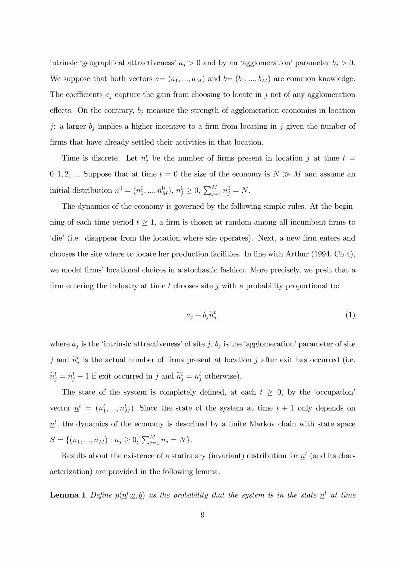
intrinsic ‘geographical attractiveness’ aj > 0 and by an ‘agglomeration’ parameter bj > 0.

We suppose that both vectors a= (a1, ..., aM) and b= (b1, ..., bM) are common knowledge.

The coefficients aj capture the gain from choosing to locate in j net of any agglomeration

effects. On the contrary, bj measure the strength of agglomeration economies in location

j: a larger bj implies a higher incentive to a firm from locating in j given the number of

firms that have already settled their activities in that location.

Time is discrete. Let ntj be the number of firms present in location j at time t =

0, 1, 2, .... Suppose that at time t = 0 the size of the economy is N À M and assume an

initial distribution n0 = (n01, ..., n0M), n

0j ≥ 0,

PMj=1 n

0j = N .

The dynamics of the economy is governed by the following simple rules. At the begin-

ning of each time period t ≥ 1, a firm is chosen at random among all incumbent firms to

‘die’ (i.e. disappear from the location where she operates). Next, a new firm enters and

chooses the site where to locate her production facilities. In line with Arthur (1994, Ch.4),

we model firms’ locational choices in a stochastic fashion. More precisely, we posit that a

firm entering the industry at time t chooses site j with a probability proportional to:

aj + bjentj, (1)

where aj is the ‘intrinsic attractiveness’ of site j, bj is the ‘agglomeration’ parameter of site

j and entj is the actual number of firms present at location j after exit has occurred (i.e.

entj = nt

j − 1 if exit occurred in j and entj = nt

j otherwise).

The state of the system is completely defined, at each t ≥ 0, by the ‘occupation’

vector nt = (nt1, ..., n

tM). Since the state of the system at time t + 1 only depends on

nt, the dynamics of the economy is described by a finite Markov chain with state space

S = {(n1, ..., nM) : nj ≥ 0,PM

j=1 nj = N}.Results about the existence of a stationary (invariant) distribution for nt (and its char-

acterization) are provided in the following lemma.

Lemma 1 Define p(nt;a, b) as the probability that the system is in the state nt at time

9

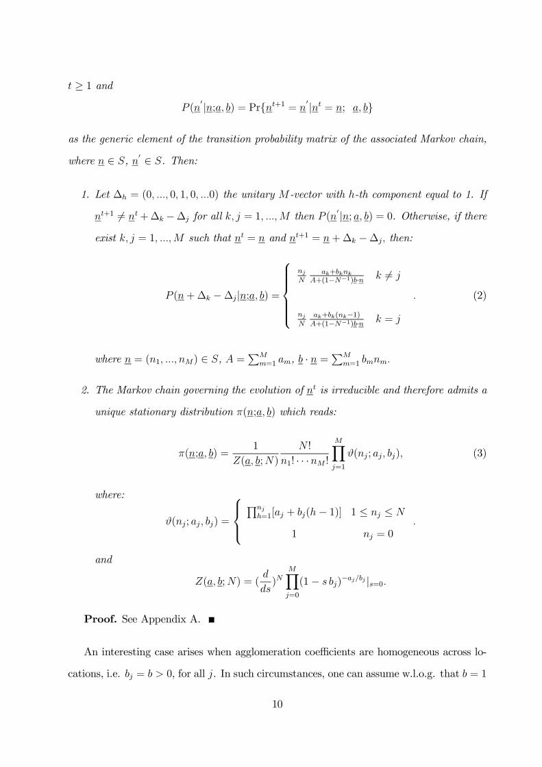
t ≥ 1 andP (n

0 |n;a, b) = Pr{nt+1 = n0|nt = n; a, b}

as the generic element of the transition probability matrix of the associated Markov chain,

where n ∈ S, n0 ∈ S. Then:

1. Let ∆h = (0, ..., 0, 1, 0, ...0) the unitary M-vector with h-th component equal to 1. If

nt+1 6= nt+∆k −∆j for all k, j = 1, ...,M then P (n0 |n; a, b) = 0. Otherwise, if there

exist k, j = 1, ...,M such that nt = n and nt+1 = n +∆k −∆j, then:

P (n+∆k −∆j|n;a, b) =

nj

Nak+bknk

A+(1−N−1)b·n k 6= j

nj

Nak+bk(nk−1)A+(1−N−1)b·n k = j

. (2)

where n = (n1, ..., nM) ∈ S, A =PM

m=1 am, b · n =PM

m=1 bmnm.

2. The Markov chain governing the evolution of nt is irreducible and therefore admits a

unique stationary distribution π(n;a, b) which reads:

π(n;a, b) =1

Z(a, b;N)

N !

n1! · · ·nM !

MYj=1

ϑ(nj; aj, bj), (3)

where:

ϑ(nj; aj, bj) =

Qnj

h=1[aj + bj(h− 1)]1

1 ≤ nj ≤ N

nj = 0.

and

Z(a, b;N) = (d

ds)N

MYj=0

(1− s bj)−aj/bj |s=0.

Proof. See Appendix A.

An interesting case arises when agglomeration coefficients are homogeneous across lo-

cations, i.e. bj = b > 0, for all j. In such circumstances, one can assume w.l.o.g. that b = 1

10

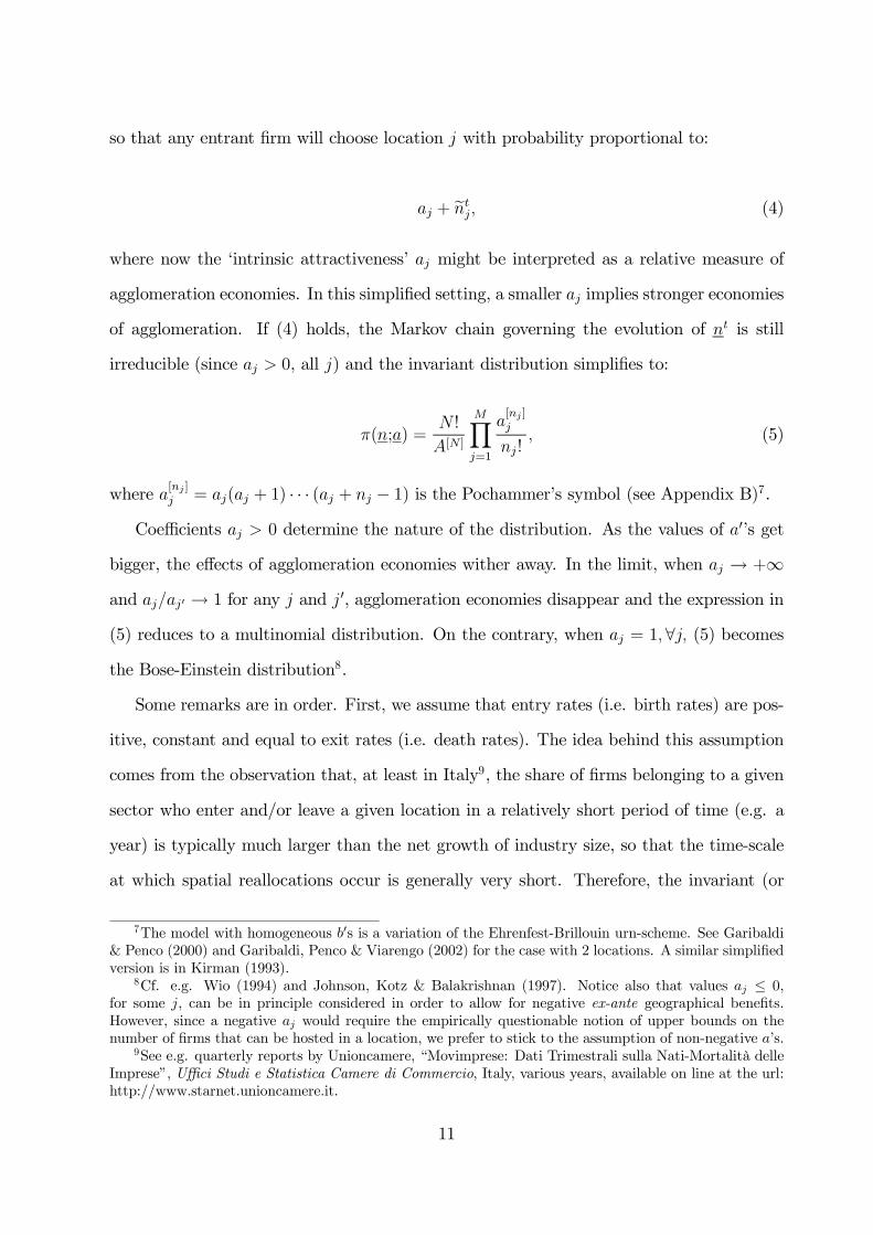
so that any entrant firm will choose location j with probability proportional to:

aj + entj, (4)

where now the ‘intrinsic attractiveness’ aj might be interpreted as a relative measure of

agglomeration economies. In this simplified setting, a smaller aj implies stronger economies

of agglomeration. If (4) holds, the Markov chain governing the evolution of nt is still

irreducible (since aj > 0, all j) and the invariant distribution simplifies to:

π(n;a) =N !

A[N ]

MYj=1

a[nj ]j

nj!, (5)

where a[nj ]j = aj(aj + 1) · · · (aj + nj − 1) is the Pochammer’s symbol (see Appendix B)7.

Coefficients aj > 0 determine the nature of the distribution. As the values of a0’s get

bigger, the effects of agglomeration economies wither away. In the limit, when aj → +∞and aj/aj0 → 1 for any j and j 0, agglomeration economies disappear and the expression in

(5) reduces to a multinomial distribution. On the contrary, when aj = 1,∀j, (5) becomesthe Bose-Einstein distribution8.

Some remarks are in order. First, we assume that entry rates (i.e. birth rates) are pos-

itive, constant and equal to exit rates (i.e. death rates). The idea behind this assumption

comes from the observation that, at least in Italy9, the share of firms belonging to a given

sector who enter and/or leave a given location in a relatively short period of time (e.g. a

year) is typically much larger than the net growth of industry size, so that the time-scale

at which spatial reallocations occur is generally very short. Therefore, the invariant (or

7The model with homogeneous b0s is a variation of the Ehrenfest-Brillouin urn-scheme. See Garibaldi& Penco (2000) and Garibaldi, Penco & Viarengo (2002) for the case with 2 locations. A similar simplifiedversion is in Kirman (1993).

8Cf. e.g. Wio (1994) and Johnson, Kotz & Balakrishnan (1997). Notice also that values aj ≤ 0,for some j, can be in principle considered in order to allow for negative ex-ante geographical benefits.However, since a negative aj would require the empirically questionable notion of upper bounds on thenumber of firms that can be hosted in a location, we prefer to stick to the assumption of non-negative a’s.

9See e.g. quarterly reports by Unioncamere, “Movimprese: Dati Trimestrali sulla Nati-Mortalità delleImprese”, Uffici Studi e Statistica Camere di Commercio, Italy, various years, available on line at the url:http://www.starnet.unioncamere.it.

11

equilibrium) distributions in (3) and (5) does not necessarily depict a long-run state as-

sociated to some ‘old’ or ‘mature’ industry. Since each entry/exit decision made by any

one firm constitutes one time-step in the model, our invariant distributions describe the

state of the system after a sufficient large number of spatial reallocation events have taken

place (which may well imply a relatively short real-time horizon). Invariant distributions

can then be directly compared with cross-section empirical data because they describe a

system which, for short real-time horizons, always appears in its equilibrium state10.

Second, and relatedly, we suppose that any firm remains in her location until she even-

tually exits from the industry. Individual locational choices might then be interpreted

as being irreversible. However, one-step transition probabilities computed in (2) are also

consistent with an alternative locational process involving reversible choices wherein: (i)

there is a constant population of N firms (no entry/exit); (ii) in each time period a ran-

domly drawn firm is allowed to switch location with probabilities proportional to (1), with

aj > 0 for all j. In both cases, the size of the industry is constant (equal to N) through-

out the whole process because the net growth rate is zero. Therefore, the impact of the

noise introduced in the system by any single additional decision (either due entry/exit or

between-location switches), albeit quite small, does not become negligible as t becomes

large. Thus, the equilibrium behavior of the system can be described, unlike models based

on Polya-urn schemes, by a non degenerate stationary distribution.

In the next Section, we will test the predictions of the model against data on geograph-

ical distribution of firms across Italian industrial districts. As a preliminary exercise, we

will focus on the case of homogeneous agglomeration coefficients (bj = b > 0), and em-

ploy (5) to test for the existence of persistence differences in the strength of agglomeration

economies among industrial sectors.

10Cf. also Appendix C for an interpretation of this property in terms of Polya-urn schemes. Long-termmodifications in the industrial structure might be instead captured by allowing a and b coefficients tochange across subsequent phases of industry evolution, albeit in a time-scale much longer than the onerelated to spatial reallocation decisions (i.e. indexed by t).

12

4 Agglomeration Economies and Industrial Sectors:

An Application to Italian Data

In this Section we shall attempt to address the following questions. First : Do theoretical

distributions (derived from the model presented above) adequately replicate, for each given

sector, the observed frequency distributions of firms across locations? Second : What is the

statistical impact of intesectoral differences on the dynamics of spatial concentration?

Note that in order to start answering the latter question, one ought to disentangle

two basic factors jointly contributing to the observed sector-specificities in agglomera-

tion patterns, namely: (i) agglomeration drivers which, for any given sector, are location-

specific and generate agglomeration benefits due to dynamic increasing returns to concen-

tration (e.g. ex-ante differences across geographical locations, economy-wide agglomeration

spillovers which cumulatively act upon the existing concentration patterns, etc.); (ii) ag-

glomeration drivers that are entirely sector-specific and promote concentration across all

geographical locations (e.g. thanks to economies of agglomeration forces that are intrinsi-

cally related to the way knowledge is accumulated, innovations are generated, etc.).

In this perspective, we present here a preliminary study focusing on four sectors: (a)

leather products; (b) transport equipment; (c) electronics; (d) financial intermediation.

The choice is motivated by the observation that these industries display a large inter-

sectoral variation as to their patterns of innovation and learning regimes, as well as the

average sizes of their BUs and their competition patterns. More precisely, according to

the descriptive taxonomy of industrial sectors firstly proposed by Pavitt (1984) and sub-

sequently developed in Malerba & Orsenigo (1996) and Marsili (2001), these industries

belong to four distinct groups (cf. also Table 1).

In Pavitt’s terminology, the leather industry - with the partial exception of ‘fashion

products’ - might be classified as a ‘supplier dominated’ (SD) sector, characterized by

relatively small firms whose innovative opportunities largely stem from external loci of

innovation (e.g. intermediate and capital inputs produced elsewhere). SD industries usu-

13

ally involve high product differentiation and include most of the so-called “made-in-Italy”

activities (e.g. textiles, clothing, furniture, toys, etc.).

Transport equipment is a standard ‘scale-intensive’ (SI ) sector, wherein large firms

generate (both internally and thanks to ‘specialized suppliers’) innovation in production

processes and, together, master the design and production of quite complex artifacts.

Electronics typically belongs to the class of ‘science-based’ (SB) sectors. Here inno-

vation in both products and processes is largely generated in R&D departments of firms

which often maintain strong links with universities and research centers.

Finally, financial intermediation activities are ‘information intensive’ (II ) sectors, which

share with science-based industry the locus of innovation (R&D departments) and the

sources of innovative opportunities (universities and research centers). However, II sectors

typically differ from SB ones as to the means of appropriating the economic rents from

their innovations. While science-based industries typically appropriate innovations through

patents and lead times of innovators vis-à-vis would-be imitators, information intensive

ones comparatively take more advantage of the tacitness of their knowledge bases (cf.

Malerba & Orsenigo (1996)).

The conjecture that we preliminary test in this work is that intersectoral differences

in the patterns of innovation creation, innovation flows and learning regimes, as proxied

by Pavitt’s categorization, map into different degrees of local agglomeration economies,

once differences due to location-specific agglomeration effects have been factored out. It is

indeed likely that firms locational choices are affected in quite different ways by different

appropriability means, distinct sources of innovation sources/types, as well as different

channels through which technological information locally spills over. We suggest that such

spatially local, sector-specific, drivers might be able to account for the observed differences

of agglomeration patterns across industries.

Data and Methodology

The exercise employs a database provided by the Italian Statistical Office (ISTAT) from

14

the Census of Manufacturers and Services. Data contain observations about more than half

a million business units (BUs), i.e. local plants. Each observation identifies the location

of the BUs at a given point of time (end of 1996), as well as the industrial sector where it

operates. Observations refer to L = 31 industrial sectors11 while locations correspond to

M = 784 “local systems of labor mobility” (LSLM) (see footnote 6).

Let ni,l be the number of BUs in LSLM i operating in sector l. Denote with n.,l the

number of BUs operating in sector l and with ni,. the total number of BUs belonging to i-th

LSLM. Since a standard maximum likelihood procedure is not viable12, we shall estimate

coefficients ail, for any given sector l, in two benchmark cases:

1. ail are homogeneous across locations, i.e. ail = αl, where αl > 0 is a sector-specific

parameter;

2. ail are heterogeneous across locations and ail = γl · θi|l, where γl is a sector-specific

parameter and θi|l, for any given sector, is a location-specific parameter.

Notice that in the case 1. one is assuming that location-specific agglomeration drivers

are homogeneous across LSLM. Under this hypothesis, BUs belonging to any given sector l

would choose any given geographical site with equal probability. On the other hand, in the

case 2. one assumes that the geographical attractiveness of any site i can be decomposed

into a factor that accounts for location- (and possibly sector-) specific (i.e. θi|l) local

attractiveness and a strictly sector-specific factor accounting for activity-specific increasing

returns to agglomeration (i.e. γl).

We estimate θi|l by using data about all sectors different from l, which are assumed to be

exogenous with respect to the data generation process postulated in the single-sector model.

Hence, sector distributions, in both case 1. and 2., will depend on a single parameter (αl

or γl) that can be in turn estimated by a standard best-fit procedure (e.g. minimization

of chi-square test between theoretical and empirical distributions).11Data about industrial sectors are disaggregated according to the Italian ATECO 91 classification

which corresponds to the 2-digit ISIC (Rev. 3) classification.12Unfortunately, data about sufficiently long time series of homogeneous observations is still not available

at the appropriate disaggregated level.

15

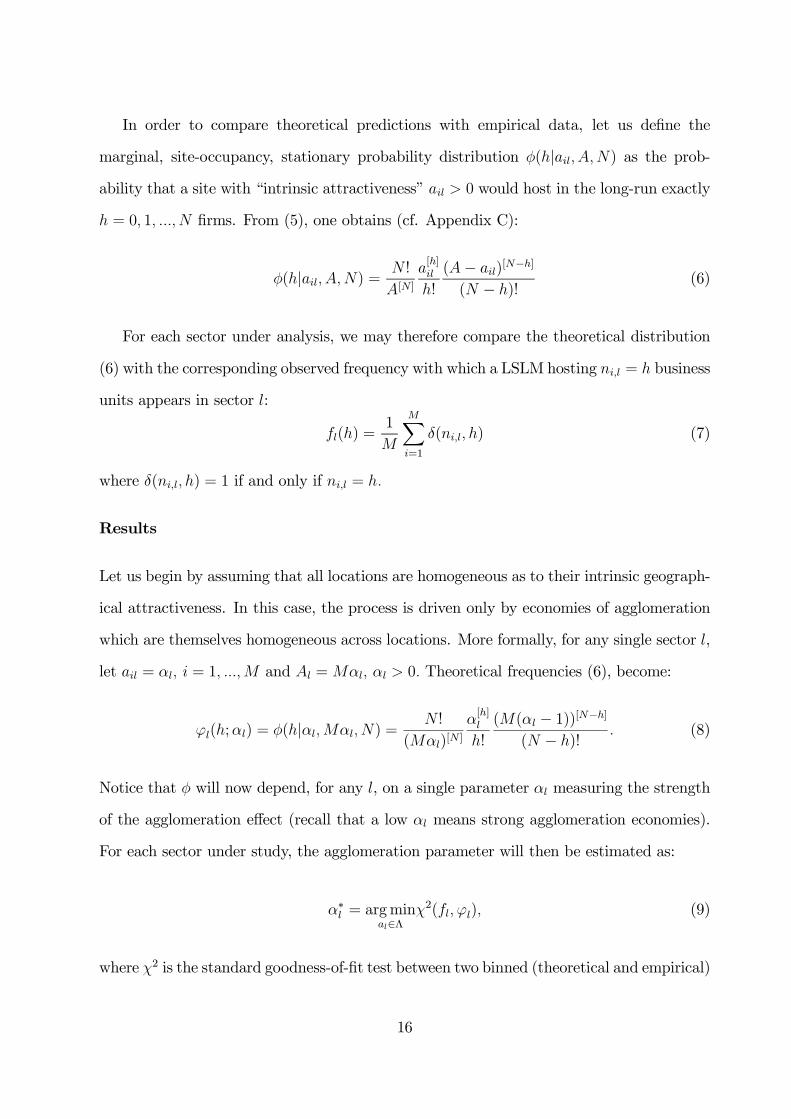
In order to compare theoretical predictions with empirical data, let us define the

marginal, site-occupancy, stationary probability distribution φ(h|ail, A,N) as the prob-ability that a site with “intrinsic attractiveness” ail > 0 would host in the long-run exactly

h = 0, 1, ..., N firms. From (5), one obtains (cf. Appendix C):

φ(h|ail, A,N) = N !

A[N ]a[h]il

h!

(A− ail)[N−h]

(N − h)!(6)

For each sector under analysis, we may therefore compare the theoretical distribution

(6) with the corresponding observed frequency with which a LSLM hosting ni,l = h business

units appears in sector l:

fl(h) =1

M

MXi=1

δ(ni,l, h) (7)

where δ(ni,l, h) = 1 if and only if ni,l = h.

Results

Let us begin by assuming that all locations are homogeneous as to their intrinsic geograph-

ical attractiveness. In this case, the process is driven only by economies of agglomeration

which are themselves homogeneous across locations. More formally, for any single sector l,

let ail = αl, i = 1, ...,M and Al =Mαl, αl > 0. Theoretical frequencies (6), become:

ϕl(h;αl) = φ(h|αl,Mαl, N) =N !

(Mαl)[N ]α[h]l

h!

(M(αl − 1))[N−h]

(N − h)!. (8)

Notice that φ will now depend, for any l, on a single parameter αl measuring the strength

of the agglomeration effect (recall that a low αl means strong agglomeration economies).

For each sector under study, the agglomeration parameter will then be estimated as:

α∗l = argminal∈Λ

χ2(fl, ϕl), (9)

where χ2 is the standard goodness-of-fit test between two binned (theoretical and empirical)

16

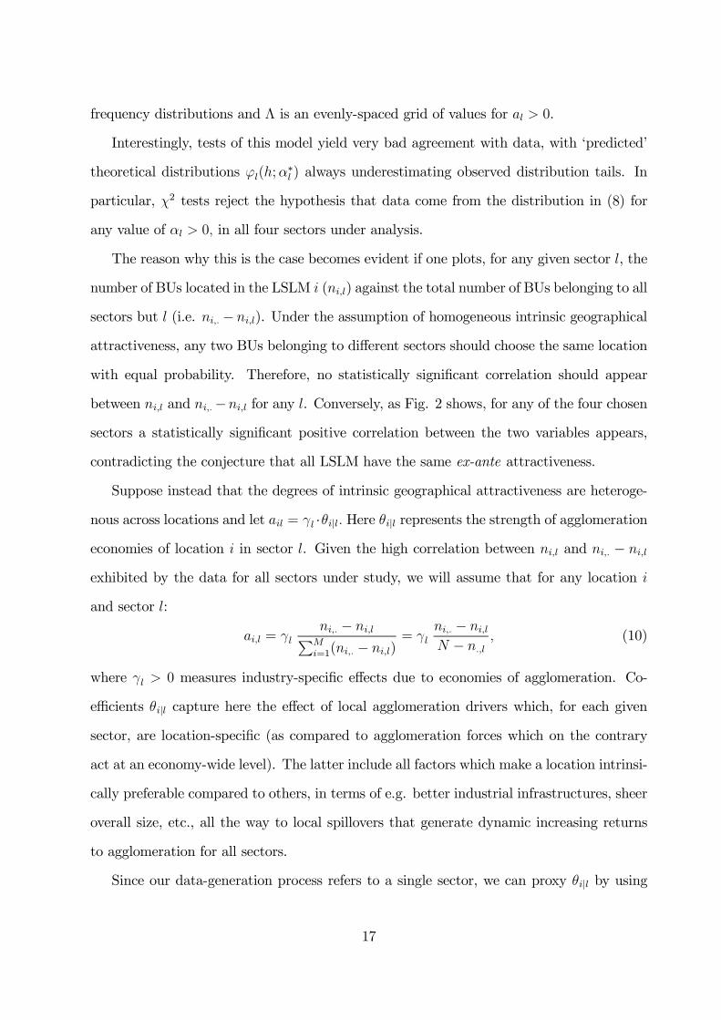
frequency distributions and Λ is an evenly-spaced grid of values for al > 0.

Interestingly, tests of this model yield very bad agreement with data, with ‘predicted’

theoretical distributions ϕl(h;α∗l ) always underestimating observed distribution tails. In

particular, χ2 tests reject the hypothesis that data come from the distribution in (8) for

any value of αl > 0, in all four sectors under analysis.

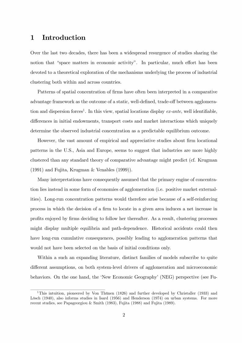
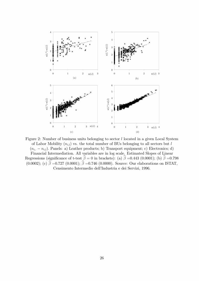
The reason why this is the case becomes evident if one plots, for any given sector l, the

number of BUs located in the LSLM i (ni,l) against the total number of BUs belonging to all

sectors but l (i.e. ni,.− ni,l). Under the assumption of homogeneous intrinsic geographical

attractiveness, any two BUs belonging to different sectors should choose the same location

with equal probability. Therefore, no statistically significant correlation should appear

between ni,l and ni,.−ni,l for any l. Conversely, as Fig. 2 shows, for any of the four chosen

sectors a statistically significant positive correlation between the two variables appears,

contradicting the conjecture that all LSLM have the same ex-ante attractiveness.

Suppose instead that the degrees of intrinsic geographical attractiveness are heteroge-

nous across locations and let ail = γl ·θi|l. Here θi|l represents the strength of agglomerationeconomies of location i in sector l. Given the high correlation between ni,l and ni,. − ni,l

exhibited by the data for all sectors under study, we will assume that for any location i

and sector l:

ai,l = γl

ni,. − ni,lPMi=1(ni,. − ni,l)

= γl

ni,. − ni,l

N − n.,l, (10)

where γl > 0 measures industry-specific effects due to economies of agglomeration. Co-

efficients θi|l capture here the effect of local agglomeration drivers which, for each given

sector, are location-specific (as compared to agglomeration forces which on the contrary

act at an economy-wide level). The latter include all factors which make a location intrinsi-

cally preferable compared to others, in terms of e.g. better industrial infrastructures, sheer

overall size, etc., all the way to local spillovers that generate dynamic increasing returns

to agglomeration for all sectors.

Since our data-generation process refers to a single sector, we can proxy θi|l by using

17

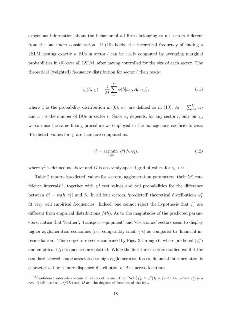
exogenous information about the behavior of all firms belonging to all sectors different

from the one under consideration. If (10) holds, the theoretical frequency of finding a

LSLM hosting exactly h BUs in sector l can be easily computed by averaging marginal

probabilities in (6) over all LSLM, after having controlled for the size of each sector. The

theoretical (weighted) frequency distribution for sector l then reads:

ψl(h; γl) =1

M

MXi=1

φ(h|ai,l, Al, n.,l), (11)

where φ is the probability distribution in (6), ai,l are defined as in (10), Al =PM

i=1 ai,l

and n.,l is the number of BUs in sector l. Since ψl depends, for any sector l, only on γl,

we can use the same fitting procedure we employed in the homogenous coefficients case.

‘Predicted’ values for γl are therefore computed as:

γ∗l = argminγl∈G

χ2(fl, ψl), (12)

where χ2 is defined as above and G is an evenly-spaced grid of values for γl > 0.

Table 2 reports ‘predicted’ values for sectoral agglomeration parameters, their 5% con-

fidence intervals13, together with χ2 test values and tail probabilities for the difference

between ψ∗l = ψl(h; γ∗l ) and fl. In all four sectors, ‘predicted’ theoretical distributions ψ

∗l

fit very well empirical frequencies. Indeed, one cannot reject the hypothesis that ψ∗l are

different from empirical distributions fl(h). As to the magnitudes of the predicted param-

eters, notice that ‘leather’, ‘transport equipment’ and ‘electronics’ sectors seem to display

higher agglomeration economies (i.e. comparably small γ’s) as compared to ‘financial in-

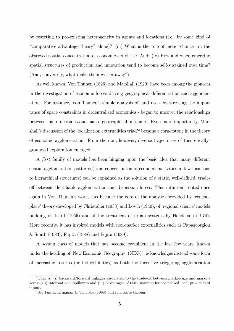
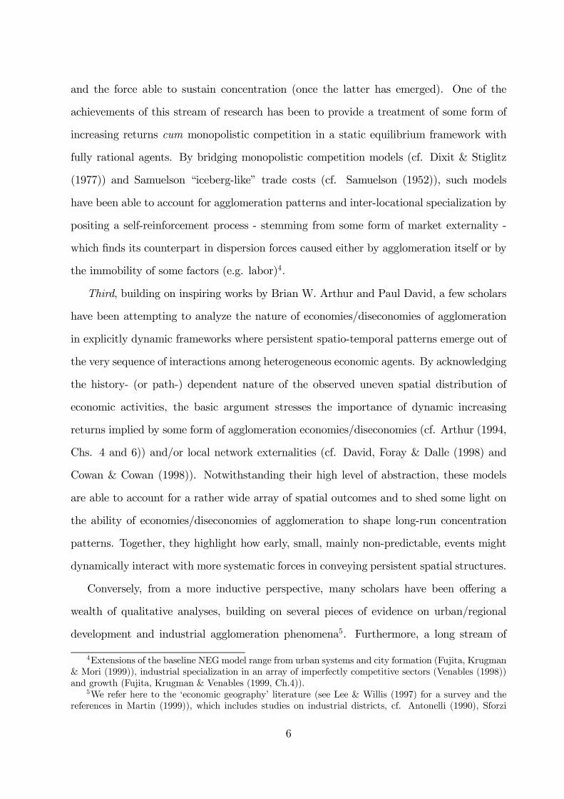
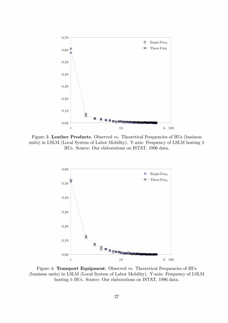
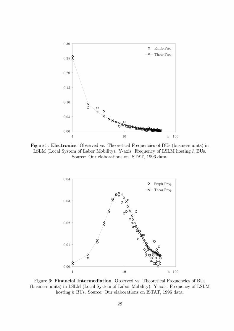
termediation’. This conjecture seems confirmed by Figs. 3 through 6, where predicted (ψ∗l )

and empirical (fl) frequencies are plotted. While the first three sectors studied exhibit the

standard skewed shape associated to high agglomeration forces, financial intermediation is

characterized by a more dispersed distribution of BUs across locations.

13Confidence intervals contain all values of γl such that Prob{χ2D > χ2(fl, ψl)} < 0.05, where χ2D is a

r.v. distributed as a χ2(D) and D are the degrees of freedom of the test.

18

In order to test whether estimated coefficients statistically differ across sectors, we

performed χ2 tests for the difference between any two distributions. We first test whether

any two ‘predicted’ distributions are different. Results reported in Table 3 show that

theoretical distributions ψ∗l are all statistically different from each other. Notice, however,

that confidence intervals for γ∗l partly overlap (see Table 2), especially as far as ‘leather’

and ‘transport equipment’ sectors are concerned. Therefore, to further explore if estimated

γ’s really differ between sectors, we compared any two distributions ψ∗l1 and ψl2(h; γ∗l1), i.e.

the distribution of sector l2 6= l1 computed employing the ‘predicted’ parameter value for

sector l1. If they statistically differ, then one might reasonably conclude that γ∗l1 6= γ∗l2 .

Results reported in Table 4 confirm that ‘financial intermediation’ exhibits agglomera-

tion economies statistically lower than the other three sectors. Furthermore, ‘electronics’

appears to display intermediate values of γ’s, while ‘leather’ and ‘transport equipment’ are

characterized by high (but not statistically different) agglomeration strength.

These results are in line with qualitative analyses on the relationships between the

intersectoral patterns of innovation/learning regimes and geographical concentration of

economic activities (cf. inter alia Antonelli (1994)). Agglomeration economies may be

expected to be relevant in SI and SD sectors (represented here indeed by ‘leather’ and

‘transport equipment’), albeit for different reasons. ‘Scale intensive’ sectors are likely to

involve hierarchical relations among firms, leading to geographical clustering characterized

by an “oligopolistic core” together with subcontracting networks. Conversely, different

drivers might lead to observationally similar statistical effects in those sectors which Pavitt

(1984) calls ‘supplier dominated’. The forces fueling many Italian industrial districts,

mostly featuring in this category, point at processes of inter-firm division of labor, at

knowledge complementarities, and at various district-specific institutional arrangements as

factors underlying agglomeration (cf. for instance Brusco (1982) and Piore & Sabel (1984)).

Agglomeration economies should also appear significant in SB sectors, due to ‘Silicon Val-

ley’ effects based on knowledge complementarities and on particular institutions fueling

“exogenous science”. However, as already noted in Bottazzi et al. (2002), science-based

19

sectors do not display in Italy striking agglomeration effects, probably due to the under-

lying weakness of ‘fueling’ research institutions, with nothing even vaguely comparable to

Stanford, UC Berkeley or MIT. Finally, firms belonging to II industries (e.g. banks and in-

surance companies) do not appear to enjoy important agglomeration economies. Therefore,

at least in our benchmark II sector, agglomeration economies implied by the existence of

large fixed costs associated to local provision of specialized intermediate goods (e.g. related

to extensive adoption of information and communication technology goods and services)

seem to be overcome by ‘monopolistically competitive’ strategies of branch location near

the customers (see Fujita & Hamaguchi (2001)).

5 Conclusions

Economies of agglomeration have been shown to play a key role in the emergence of rel-

atively stable patterns of industrial clustering. However, existing theoretical endeavours

attempting to explain industrial concentration on the basis of some form of dynamic in-

creasing returns to agglomeration have been largely neglecting the vast amount of empirical

evidence about inter-sectoral differences in the patterns of spatial activity.

In this paper, we argued that cross-sectional differences in agglomeration forces might

be (at least partly) explained by underlying differences in the processes of firms’ technolog-

ical and organizational learning. We presented a very simple model of industrial clustering

in which adaptive firms make locational choices in presence of agglomeration economies.

The latter stem from both standard comparative advantage arguments (making some lo-

cations inherently more attractive than others) and dynamic increasing returns to scale in

agglomeration which can be both sector- and industry-specific. We tested the predictions

of the model about the long-run distribution of the size of spatial clusters against data on

Italian ‘local system of labor mobility’ (i.e. a proxy for industrial districts).

In each sector under analysis, the accordance of theoretical predictions with data is quite

high, with statistically significant, sector- and location-specific, economies of agglomera-

20

tion. In turn, underlying differences in the modes of innovative exploration and knowledge

accumulation, we suggest, are likely to map into sectoral specificities in the strength of

geographical clustering.

Of course one may think of several ways forward with respect to the foregoing analysis.

First, our basic conjecture on the role of technological specificities as determinants of the

intensity of agglomeration, if any, is going to be fully corroborated only by studying many

more sectors, possibly in different countries. Second, one may incorporate explicit local

interactions among firms and non-linear formulations of the location probabilities. Third,

it would be interesting to consider inter-sectoral interactions in location patterns.

Existing evidence does suggest widespread phenomena of clustering of innovation activ-

ities (cf. Cowan & Cowan (1998) and Brusco (1982), among others). Moreover, technology-

specific interactions between location of innovative activities and location of production in

the case of multinational corporations has been identified by Cantwell and collaborators (see

e.g. Cantwell (1989) and Feldman (1994)). The foregoing study is, in many respects, com-

plementary to such investigations and, hopefully, moves some steps ahead toward bridging

the geography of location with the economics and geography of innovation.

21

ReferencesAntonelli, C. (1990), ‘Induced adoption and externalities in the regional diffusion of infor-

mation technology’, Regional Studies 24(1), 31—40.

Antonelli, C. (1994), ‘Technology districts, localized spillovers, and productivity growth:The italian evidence on technological externalities in core regions’, International Re-view of Applied Economics 12, 18—30.

Arthur, W. (1994), Increasing returns and path-dependency in economics, University ofMichigan Press, Ann Arbor.

Beccattini, G. (1990), The marshallian industrial district as a socio-economic notion, inF. Pyke, G. Beccattini & W. Sengenberger, eds, ‘Industrial Districts and Inter-FirmCooperation in Italy’, Geneva, International Inst. for Labour studies.

Bottazzi, G., Dosi, G. & Fagiolo, G. (2002), On the ubiquitous nature of the agglomera-tion economies and their diverse determinants: Some notes, in A. Quadrio Curzio &M. Fortis, eds, ‘Complexity and Industrial Clusters: Dynamics and Models in Theoryand Practice’, Heidelberg, Physica-Verlag.

Brusco, S. (1982), ‘The emilian model: productive decentralisation and social integration’,Cambridge Journal of Economics 6, 167—184.

Cantwell, J. (1989), Technological Innovations and Multinational Corporations, Oxford,Basic Books.

Cantwell, J. & Iammarino, S. (1998), ‘Mncs, technological innovation and regional systemsin the eu: Some evidence in the italian case’, International Journal of the Economicsof Business 5, 383—408.

Christaller, W. (1933), Central Places in Southern Germany, Jena, Fischer.

Cowan, R. & Cowan, W. (1998), ‘On clustering in the location of rd: Statics and dynamics’,Economics of Innovation and New Technology 6, 201—229.

David, P., Foray, D. & Dalle, J. (1998), ‘Marshallian externalities and the emergenceof spatial stability and technological enclaves’, Economics of Innovation and NewTechnology 6, 147—182.

Dixit, A. & Stiglitz, J. (1977), ‘Monopolistic competition and optimum product diversity’,American Economic Review 67, 297—308.

Dosi, G. (1988), ‘Sources, procedures and microeconomic effects of innovation’, Journal ofEconomic Literature 26, 126—171.

Feldman, M. (1994), The Geography of Innovation, Boston, Kluwer Academic Publishers.

Fujita, M. (1988), ‘A monopolistic competition model of spatial agglomeration’, RegionalScience and Urban Economics 18(1), 87—124.

22

Fujita, M. (1989), Urban Economic Theory. Land Use and City Size, Cambridge, MA,Cambridge University Press.

Fujita, M. & Hamaguchi, N. (2001), ‘Intermediate goods and the spatial structure of aneconomy’, Regional Science and Urban Economics 31, 79—109.

Fujita, M., Krugman, P. & Mori, T. (1999), ‘On the evolution of hierarchical urban sys-tems’, European Economic Review 10, 339—378.

Fujita, M., Krugman, P. & Venables, A. (1999), The Spatial Economy: Cities, Regions,and International Trade, Cambridge, Massachussets, The MIT Press.

Garibaldi, U. & Penco, M. (2000), ‘Ehrenfest urn model generalized: an exact approachfor market participation models’, Statistica Applicata 12, 249—272.

Garibaldi, U., Penco, M. & Viarengo, P. (2002), Ax exact physical approach for marketparticipation models, in R. Cowan & N. Jonard, eds, ‘Heterogeneous Agents, Inter-actions, and Economic Performance’, Lecture Notes in Economics and MathematicalSystems, Berlin-Heidelberg, Springer-Verlag, Forthcoming.

Gradshteyn, I. & Ryzhik, I. (2000), Table of Integrals, Series and Products, Edited by A.Jeffrey and D. Zwillinger, New York, Academic Press.

Henderson, J. (1974), ‘The sizes and types of cities’, American Economic Review 64, 640—656.

Isard, W. (1956), Location and Space-Economy, Cambridge, Massachussets, The MITPress.

Johnson, N., Kotz, S. & Balakrishnan, N. (1997), Discrete Multivariate Distributions, NewYork, Wiley.

Kirman, A. (1993), ‘Ants, rationality and recruitment’, Quarterly Journal of Economics108, 137—156.

Krugman, P. (1991), ‘Increasing returns and economic geography’, Journal of PoliticalEconomy 99, 483—499.

Lee, R. & Willis, J. (1997), Geographies of Economies, London, Arnold.

Lösch, A. (1940), The Economics of Location, Jena, Fischer.

Malerba, F. & Orsenigo, L. (1996), ‘Technological regimes and firm behaviour’, Industrialand Corporate Change 5, 51—88.

Marshall, A. (1920), Principles of Economics, London, MacMillan.

Marsili, O. (2001), The Anatomy and Evolution of Industries: Technological Change andIndustrial Dynamics, Chelthenam, Edward Elgar.

Martin, R. (1999), ‘The new ’geographical turn’ in economics: some critical reflections’,Cambridge Journal of Economics 23, 65—91.

23

Papageorgiou, Y. & Smith, T. (1983), ‘Agglomeration and local instability of spatiallyuniform steady-states’, Econometrica 51, 1109—1119.

Pavitt, K. (1984), ‘Sectoral patterns of technical change: Towards a taxonomy and atheory’, Research Policy 13, 343—373.

Piore, M. & Sabel, C. (1984), The Second Industrial Divide: Possibilities for Prosperity,New York, Basic Books.

Rauch, J. (1993), ‘Does history matters only when it matters little ? the case of city-industry location’, The Quarterly Journal of Economics 108, 843—867.

Samuelson, P. (1952), ‘The transfer problem and transport costs: The terms of trade whenimpediments are absent’, Economic Journal 62, 278—304.

Sforzi, F. (1989), The geography of industrial districts in italy, in E. Goodman & J. Bam-ford, eds, ‘Small Firms and Industrial Districts in Italy’, London, Routledge.

Sforzi, F. (2000), Local development in the experience of italian industrial districts, inI. C. of Research, ed., ‘Geographies of Diverse Ties. An Italian Perspective’, Rome,CNR-IGU.

Venables, A. (1998), Geography and specialization: Industrial belts on a circular plain,in R. Baldwin, D. Cohen, A. Sapir & A. Venables, eds, ‘Regional Integration’, Cam-bridge, Massachussets, Cambridge University Press.

Vernon, R. (1966), ‘International investment and international trade in the product cycle’,Quarterly Journal of Economics 80, 190—207.

Von Thünen, J. (1826), Det Isolierte Staat in Beziehung auf Landwirtschaft und Nation-alokonomie, Hamburg, Perthes.

Wio, H. (1994), An Introduction to Stochastic Processes and Nonequilibrium StatisticalPhysics, Singapore, World Scientific Publishing.

24

0,00

0,04

0,08

0,0 0,5 1,0Max

%

0,00

0,20

0,40

0,60

0,0 0,1 0,2Min

%

0,00

0,03

0,06

0,0 0,5 1,0Range

%

0,00

0,07

0,14

0,0 0,2 0,4St.Dev.

%

Figure 1: Frequency distributions of MAX (Top-Left), MIN (Top-Right), RANGE(Bottom-Left) and STANDARD DEVIATION (Bottom-Right) statistics computed on

the weighted frequency profile of Italian manufacturing business units (BUs) belonging todifferent industrial sectors (2-digit disaggregation) present in each geographical locationin 1996. For each statistics S, a circle corresponding to a value s on the x-axis representsthe % of all locations for which the statistics S (computed on the weighted frequencyprofile of firms belonging to each industrial sector present in that location) is equal to s.Locations are defined in terms of Local Systems of Labor Mobility (cf. footnote 6).

Source: Our elaborations on ISTAT, Censimento Intermedio dell’Industria e dei Servizi,1996.

25

(a)

0

1

2

3

4

0 1 2 3n(i,l)

n(i,*)-n(i,l)

(b)

0

1

2

3

4

5

0 1 2 3n(i,l)

n(i,*)-n(i,l)

(c)

0

1

2

3

4

5

0 1 2 3 4n(i,l)

n(i,*)-n(i,l)

(d)

0

1

2

3

4

5

6

0 1 2 3 4n(i,l)

n(i,*)-n(i,l)

Figure 2: Number of business units belonging to sector l located in a given Local Systemof Labor Mobility (ni,l) vs. the total number of BUs belonging to all sectors but l(ni,· − ni,l). Panels: a) Leather products; b) Transport equipment; c) Electronics; d)Financial Intermediation. All variables are in log scale. Estimated Slopes of Linear

Regressions (significance of t-test bβ = 0 in brackets): (a) bβ =0.443 (0.0001); (b) bβ =0.798(0.0002); (c) bβ =0.727 (0.0001); bβ =0.746 (0.0000). Source: Our elaborations on ISTAT,

Censimento Intermedio dell’Industria e dei Servizi, 1996.

26

0,00

0,10

0,20

0,30

0,40

0,50

0,60

0,70

1 10 100h

Empir.Freq.

Theor.Freq

Figure 3: Leather Products. Observed vs. Theoretical Frequencies of BUs (businessunits) in LSLM (Local System of Labor Mobility). Y-axis: Frequency of LSLM hosting h

BUs. Source: Our elaborations on ISTAT, 1996 data.

0,00

0,10

0,20

0,30

0,40

0,50

0,60

1 10 100h

Empir.Freq.

Theor.Freq.

Figure 4: Transport Equipment. Observed vs. Theoretical Frequencies of BUs(business units) in LSLM (Local System of Labor Mobility). Y-axis: Frequency of LSLM

hosting h BUs. Source: Our elaborations on ISTAT, 1996 data.

27

0,00

0,05

0,10

0,15

0,20

0,25

0,30

1 10 100h

Empir.Freq.

Theor.Freq.

Figure 5: Electronics. Observed vs. Theoretical Frequencies of BUs (business units) inLSLM (Local System of Labor Mobility). Y-axis: Frequency of LSLM hosting h BUs.

Source: Our elaborations on ISTAT, 1996 data.

0,00

0,01

0,02

0,03

0,04

1 10 100h

Empir.Freq.

Theor.Freq.

Figure 6: Financial Intermediation. Observed vs. Theoretical Frequencies of BUs(business units) in LSLM (Local System of Labor Mobility). Y-axis: Frequency of LSLM

hosting h BUs. Source: Our elaborations on ISTAT, 1996 data.

28

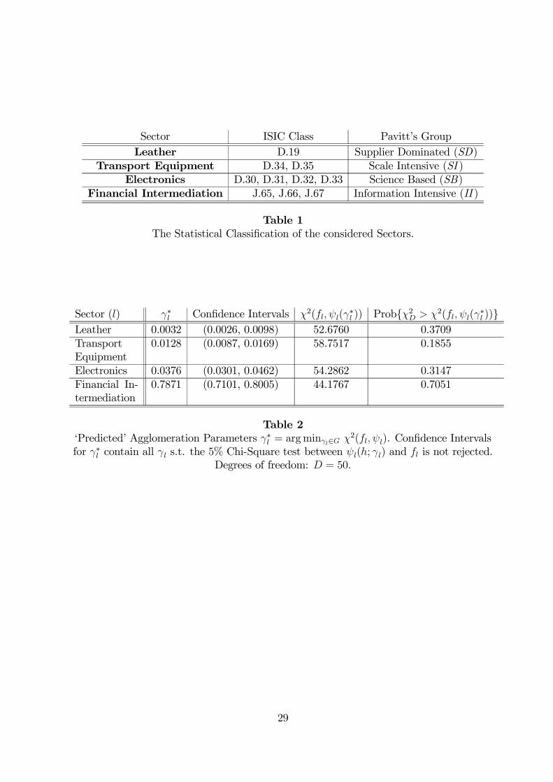
Sector ISIC Class Pavitt’s GroupLeather D.19 Supplier Dominated (SD)

Transport Equipment D.34, D.35 Scale Intensive (SI )Electronics D.30, D.31, D.32, D.33 Science Based (SB)

Financial Intermediation J.65, J.66, J.67 Information Intensive (II )

Table 1The Statistical Classification of the considered Sectors.

Sector (l) γ∗l Confidence Intervals χ2(fl, ψl(γ∗l )) Prob{χ2D > χ2(fl, ψl(γ

∗l ))}

Leather 0.0032 (0.0026, 0.0098) 52.6760 0.3709TransportEquipment

0.0128 (0.0087, 0.0169) 58.7517 0.1855

Electronics 0.0376 (0.0301, 0.0462) 54.2862 0.3147Financial In-termediation

0.7871 (0.7101, 0.8005) 44.1767 0.7051

Table 2‘Predicted’ Agglomeration Parameters γ∗l = argminγl∈G χ2(fl, ψl). Confidence Intervalsfor γ∗l contain all γl s.t. the 5% Chi-Square test between ψl(h; γl) and fl is not rejected.

Degrees of freedom: D = 50.

29

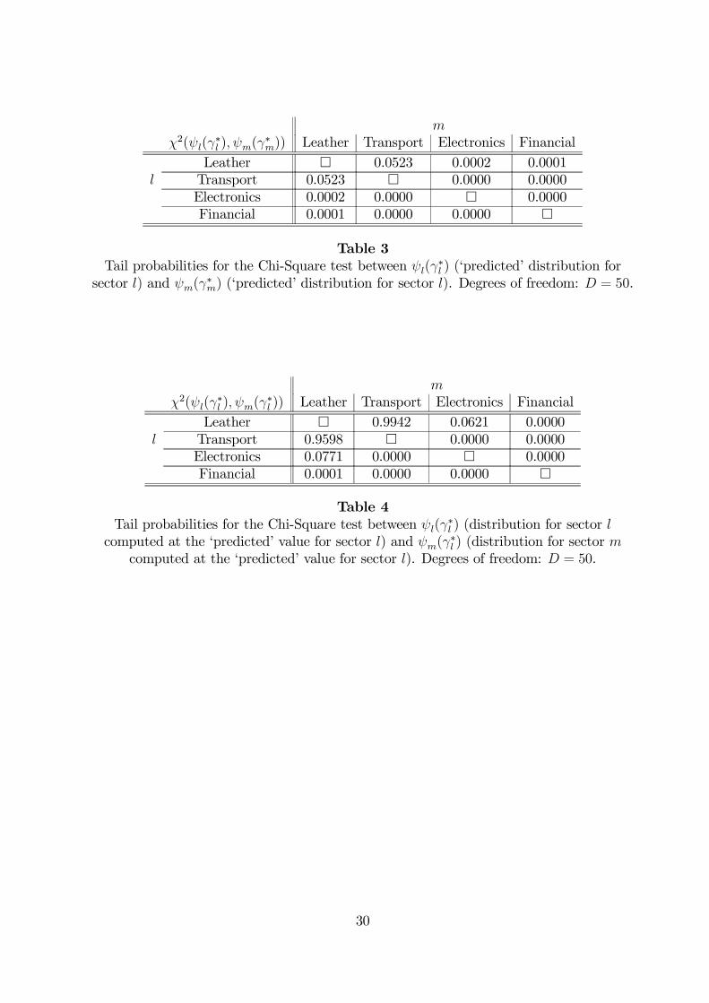
mχ2(ψl(γ

∗l ), ψm(γ

∗m)) Leather Transport Electronics Financial

Leather ¤ 0.0523 0.0002 0.0001l Transport 0.0523 ¤ 0.0000 0.0000

Electronics 0.0002 0.0000 ¤ 0.0000Financial 0.0001 0.0000 0.0000 ¤

Table 3Tail probabilities for the Chi-Square test between ψl(γ

∗l ) (‘predicted’ distribution for

sector l) and ψm(γ∗m) (‘predicted’ distribution for sector l). Degrees of freedom: D = 50.

mχ2(ψl(γ

∗l ), ψm(γ

∗l )) Leather Transport Electronics Financial

Leather ¤ 0.9942 0.0621 0.0000l Transport 0.9598 ¤ 0.0000 0.0000

Electronics 0.0771 0.0000 ¤ 0.0000Financial 0.0001 0.0000 0.0000 ¤

Table 4Tail probabilities for the Chi-Square test between ψl(γ

∗l ) (distribution for sector l

computed at the ‘predicted’ value for sector l) and ψm(γ∗l ) (distribution for sector m

computed at the ‘predicted’ value for sector l). Degrees of freedom: D = 50.

30

Appendices

A Proof of Lemma 1

Point 1. Let P (n0 |n;a, b) be the generic element of the transition matrix of the Markov

chain that describes the dynamics of the system. Moreover, let p(nt = n;a, b) the proba-

bility that the chain is in the state n at time t (in the following we will omit, for the sake

of simplicity, parameters a, b).

We have assumed that in any time period only one firm will exit her current location

and only one firm will enter one of the M locations (possibly including the one in which

exit has occurred). Therefore, given nt = n, the state at time t+1 must necessarily be such

that either (i) there exist two locations, say k0 and k00, k0 6= k00such that nk0t+1 = nk0t − 1and nk00t+1 = nk00t + 1; or (ii) nt+1 = nt, if the entrant has chosen the same location of

the exiting firm. Hence if nt+1 6= nt + ∆k − ∆j for all k, j = 1, ...,M then P (n0|n) = 0.

Otherwise, if there exist k, j = 1, ...,M such that nt = n and nt+1 = n+∆k−∆j, then for

any j, k = 1, ...,M :

Pr{n+∆k −∆j|n} = Pr{A Firm Exits from location j}·

·Pr{Entrant Chooses location k|A Firm Exits from location j}.

As the exiting firm is chosen at random from all incumbent firms then:

Pr{A Firm Exits from location j} = ntj

N.

From (1), we also have that the entrant firm will find ntk firms in any location k 6= j, while

31

(if a firm has left location j) she will find ntj − 1 firms in location j. Thus:

Pr{Entrant Chooses location k|A Firm Exits from location j} ∝

∝

ak + bkntk

ak + bk(ntk − 1)

k 6= j

k = j.

By imposing the normalizing condition:

H−1 · [MXj=1

MXk=1k 6=j

ntj

N(ak + bkn

tk) +

MXj=1

ntj

N(aj + bj(n

tj − 1))] = 1,

we easily get that

H =MXh=1

ah + (1− 1

N)

MXh=1

bhnh = A+ (1−N−1)MXh=1

bhnh. (13)

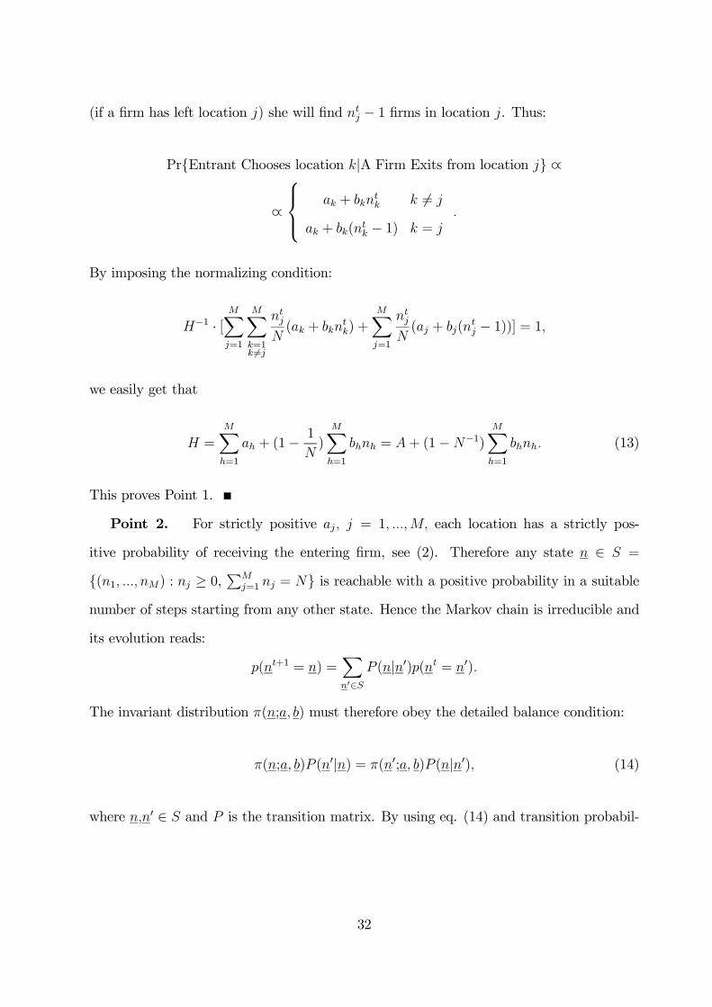
This proves Point 1.

Point 2. For strictly positive aj, j = 1, ...,M, each location has a strictly pos-

itive probability of receiving the entering firm, see (2). Therefore any state n ∈ S =

{(n1, ..., nM) : nj ≥ 0,PM

j=1 nj = N} is reachable with a positive probability in a suitablenumber of steps starting from any other state. Hence the Markov chain is irreducible and

its evolution reads:

p(nt+1 = n) =Xn0∈S

P (n|n0)p(nt = n0).

The invariant distribution π(n;a, b) must therefore obey the detailed balance condition:

π(n;a, b)P (n0|n) = π(n0;a, b)P (n|n0), (14)

where n,n0 ∈ S and P is the transition matrix. By using eq. (14) and transition probabil-

32

ities given in (2), one gets:

π(n +∆k −∆j;a, b) = π(n;a, b)nj

nk + 1

ak + bknk

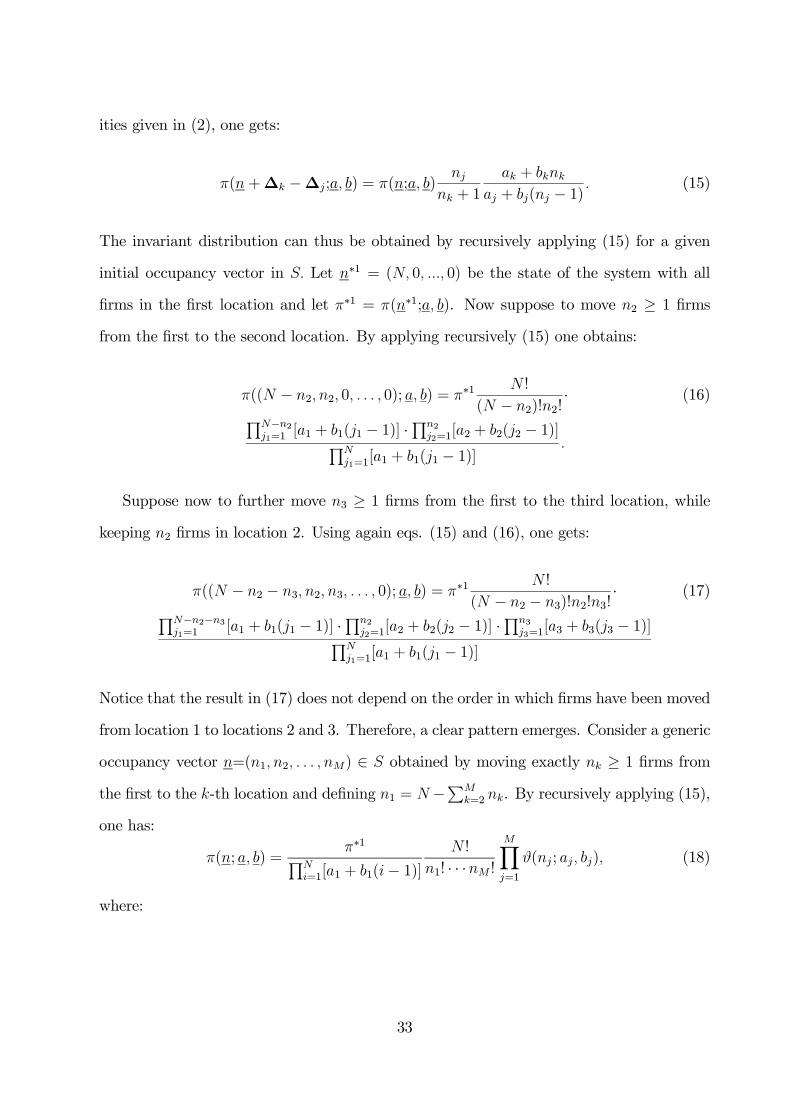
aj + bj(nj − 1) . (15)

The invariant distribution can thus be obtained by recursively applying (15) for a given

initial occupancy vector in S. Let n∗1 = (N, 0, ..., 0) be the state of the system with all

firms in the first location and let π∗1 = π(n∗1;a, b). Now suppose to move n2 ≥ 1 firms

from the first to the second location. By applying recursively (15) one obtains:

π((N − n2, n2, 0, . . . , 0); a, b) = π∗1N !

(N − n2)!n2!· (16)QN−n2

j1=1[a1 + b1(j1 − 1)] ·

Qn2j2=1

[a2 + b2(j2 − 1)]QNj1=1

[a1 + b1(j1 − 1)].

Suppose now to further move n3 ≥ 1 firms from the first to the third location, while

keeping n2 firms in location 2. Using again eqs. (15) and (16), one gets:

π((N − n2 − n3, n2, n3, . . . , 0); a, b) = π∗1N !

(N − n2 − n3)!n2!n3!· (17)QN−n2−n3

j1=1[a1 + b1(j1 − 1)] ·

Qn2j2=1

[a2 + b2(j2 − 1)] ·Qn3

j3=1[a3 + b3(j3 − 1)]QN

j1=1[a1 + b1(j1 − 1)]

Notice that the result in (17) does not depend on the order in which firms have been moved

from location 1 to locations 2 and 3. Therefore, a clear pattern emerges. Consider a generic

occupancy vector n=(n1, n2, . . . , nM) ∈ S obtained by moving exactly nk ≥ 1 firms fromthe first to the k-th location and defining n1 = N−PM

k=2 nk. By recursively applying (15),

one has:

π(n; a, b) =π∗1QN

i=1[a1 + b1(i− 1)]N !

n1! · · ·nM !

MYj=1

ϑ(nj; aj, bj), (18)

where:

33

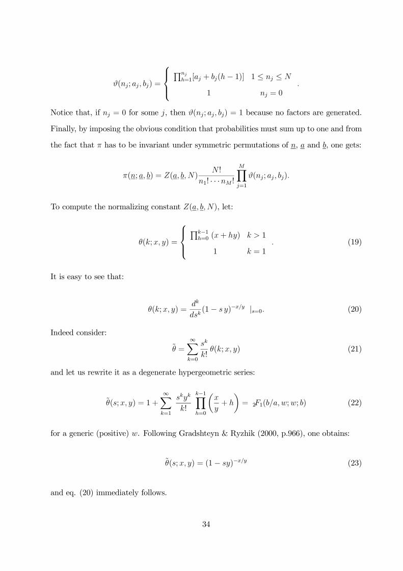
ϑ(nj; aj, bj) =

Qnj

h=1[aj + bj(h− 1)]1

1 ≤ nj ≤ N

nj = 0.

Notice that, if nj = 0 for some j, then ϑ(nj; aj, bj) = 1 because no factors are generated.

Finally, by imposing the obvious condition that probabilities must sum up to one and from

the fact that π has to be invariant under symmetric permutations of n, a and b, one gets:

π(n; a, b) = Z(a, b, N)N !

n1! · · ·nM !

MYj=1

ϑ(nj; aj, bj).

To compute the normalizing constant Z(a, b, N), let:

θ(k;x, y) =

Qk−1

h=0 (x+ hy) k > 1

1 k = 1. (19)

It is easy to see that:

θ(k;x, y) =dk

dsk(1− s y)−x/y |s=0. (20)

Indeed consider:

θ̃ =∞Xk=0

sk

k!θ(k;x, y) (21)

and let us rewrite it as a degenerate hypergeometric series:

θ̃(s;x, y) = 1 +∞Xk=1

skyk

k!

k−1Yh=0

µx

y+ h

¶= 2F1(b/a, w;w; b) (22)

for a generic (positive) w. Following Gradshteyn & Ryzhik (2000, p.966), one obtains:

θ̃(s;x, y) = (1− sy)−x/y (23)

and eq. (20) immediately follows.

34

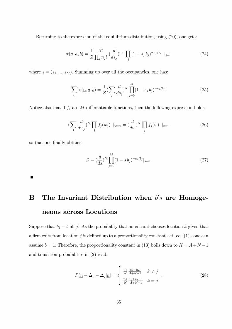
Returning to the expression of the equilibrium distribution, using (20), one gets:

π(n, a, b) =1

Z

N !Qj nj!

(d

dsj)nj

Yj

(1− sj bj)−aj/bj |s=0 (24)

where s = (s1, ..., sM). Summing up over all the occupancies, one has:

Xn

π(n, a, b) =1

Z(Xj

d

dsj)N

MYj=0

(1− sj bj)−aj/bj . (25)

Notice also that if fj are M differentiable functions, then the following expression holds:

(Xj

d

dwj)NYj

fj(wj) |w=0 = ( d

dw)NYj

fj(w) |x=0 (26)

so that one finally obtains:

Z = (d

ds)N

MYj=0

(1− s bj)−aj/bj |s=0. (27)

B The Invariant Distribution when b0s are Homoge-

neous across Locations

Suppose that bj = b all j. As the probability that an entrant chooses location k given that

a firm exits from location j is defined up to a proportionality constant - cf. eq. (1) - one can

assume b = 1. Therefore, the proportionality constant in (13) boils down to H = A+N−1and transition probabilities in (2) read:

P (n +∆k −∆j|n) =

nj

Nak+nk

A+N−1 k 6= j

nj

Nak+nk−1A+N−1 k = j

. (28)

35

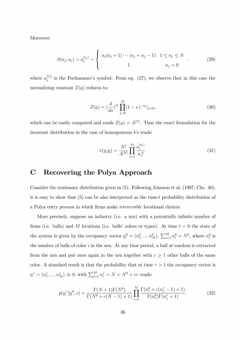
Moreover:

ϑ(nj; aj) = a[nj ]j =

aj(aj + 1) · · · (aj + nj − 1)1

1 ≤ nj ≤ N

nj = 0. (29)

where a[nj ]j is the Pochammer’s symbol. From eq. (27), we observe that in this case the

normalizing constant Z(a) reduces to:

Z(a) = (d

ds)N

MYj=0

(1− s )−aj |s=0, (30)

which can be easily computed and reads Z(a) = A[N ]. Thus the exact formulation for the

invariant distribution in the case of homogeneous b’s reads:

π(n;a) =N !

A[N ]

MYj=1

a[nj ]j

nj!. (31)

C Recovering the Polya Approach

Consider the stationary distribution given in (5). Following Johnson et al. (1997, Chs. 40),

it is easy to show that (5) can be also interpreted as the time-t probability distribution of

a Polya entry process in which firms make irreversible locational choices.

More precisely, suppose an industry (i.e. a urn) with a potentially infinite number of

firms (i.e. balls) and M locations (i.e. balls’ colors or types). At time t = 0 the state of

the system is given by the occupancy vector n0 = (n01, ..., n0M),

PMi=1 n

0i = N0, where n0i is

the number of balls of color i in the urn. At any time period, a ball at random is extracted

from the urn and put once again in the urn together with c ≥ 1 other balls of the same

color. A standard result is that the probability that at time τ > 1 the occupancy vector is

nτ = (nτ1, ..., n

τM)À 0, with

PMi=1 n

τi = N = N0 + cτ reads:

p(nτ |n0, c) = Γ(N + 1)Γ(N0)

Γ(N0 + c(N − 1) + 1)MYi=1

Γ(n0i + c(nτj − 1) + 1)

Γ(n0i )Γ(nτj + 1)

. (32)

36

If we are allowed to add only one ball at any time (i.e. c = 1), then N t = N t−1 + 1 and

(32) becomes:

p(nτ |n0) = N !

(N 0)[N ]

MYi=1

(n0j)[nτ

j ]

nτj !

, (33)

where a[x] = a(a+ 1) · · · (a+ x− 1) is the Pochammer’s symbol. Therefore, if aj = n0j , the

probability distribution (33) becomes the invariant distribution for the Ehrenfest-Brillouin

model (5). This results allows us to directly compute (using standard results for the Polya

process theory, cf. Johnson et al. (1997, Chs. 40)), the marginal probability that a site with

intrinsic benefit a will contain in the long-run exactly k firms. Indeed, the latter marginal

distribution is equal to the marginal probability that in an urn with 2 colors there will be

k balls with the first color, when in the urn there are N balls and the initial number of

balls of the first color were a, cf. eq. (6).

Notice finally that, in contrast with the process of firms locational choice presented in

Section 3, initial conditions (i.e. the number of firms initially present in each locations)

matter in the finite-time probability distribution of the Polya process. As net industry

growth rate is positive (entry rate is equal to c while exit rate is zero) locational decisions are

irreversible. Therefore, dynamic increasing returns strongly affect long-run agglomeration

patterns as early micro events may cumulatively reinforce the agglomeration benefit of

any given location, possibly overcoming ex-ante intrinsic comparative advantages. The

impact of additional perturbations caused by entry becomes progressively negligible in the

long-run, thus leading to lock-in of the system. On the other hand, the Ehrenfest-Brillouin

interpretation is consistent with always-reversible decisions: initial conditions never matter

for the invariant distribution. As the size of any individual perturbation does not die out

with time, the strength of dynamic increasing returns is much weaker than in the Polya

interpretation.

37