Maximum Likelihood estimation: Stata vs. Gauss

Index

 Motivation  Objective

 The Maximum Likelihood Method

 Capabilities: Stata vs Gauss

 Conclusions

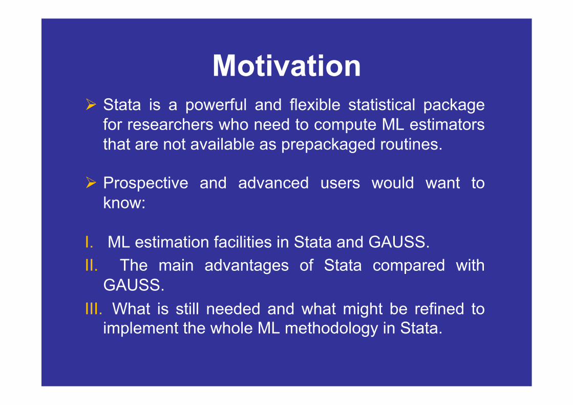
Motivation  Stata is a powerful and flexible statistical package

for researchers who need to compute ML estimators that are not available as prepackaged routines.

 Prospective and advanced users would want to know:

I.  ML estimation facilities in Stata and GAUSS. II.  The main advantages of Stata compared with

GAUSS. III.  What is still needed and what might be refined to

implement the whole ML methodology in Stata.

Objective

 The main purpose of this presentation is to

compare the ML routines and capabilities

offered by STATA and GAUSS.

The Maximum Likelihood Method

  The foundation for the theory and practice of maximum likelihood estimation is a probability model:

Where Z is the random variable distributed according to a cumulative probability distribution function F() with parameter vector from , which is the parameter space for F().

The Maximum Likelihood Method

 Typically, there is more that one variable of interest, so the model:

Describes the joint distribution of the random variables, with . Using F(), we can compute probabilities for values of the Zs given values of the parameters .

The Maximum Likelihood Method

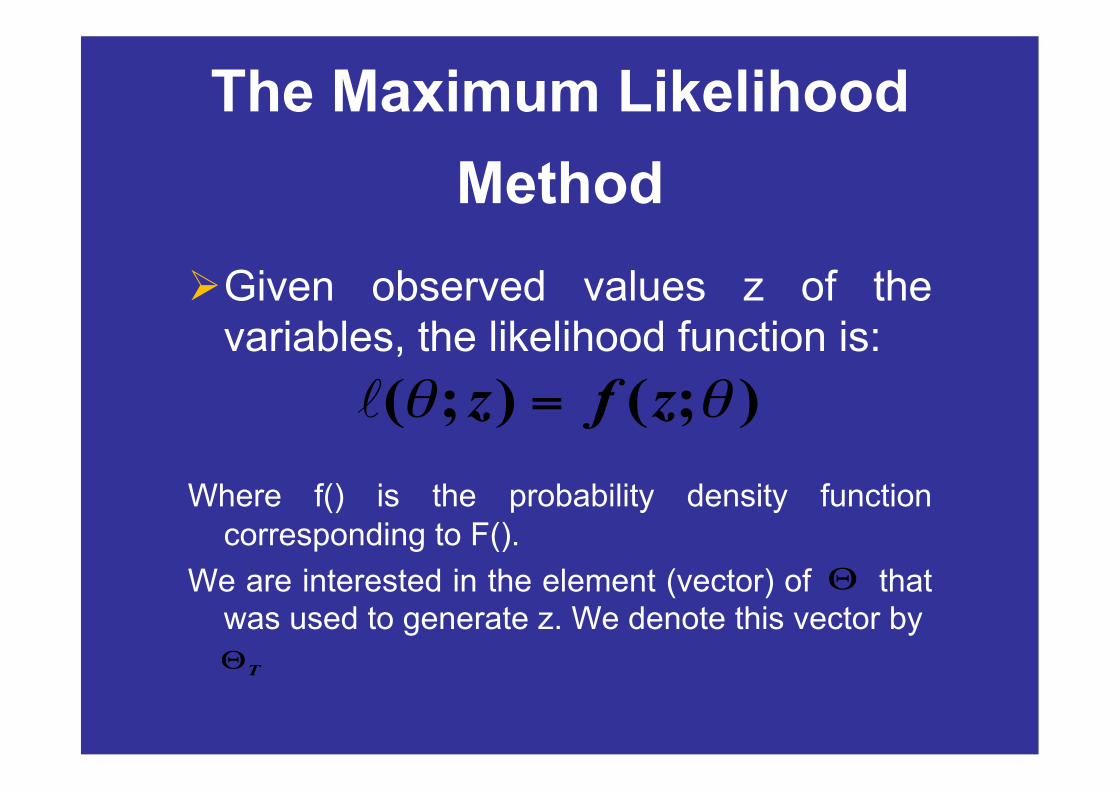
 Given observed values z of the variables, the likelihood function is:

Where f() is the probability density function corresponding to F().

We are interested in the element (vector) of that was used to generate z. We denote this vector by

The Maximum Likelihood Method

 Data typically consist of multiple observations on relevant variables, so we will denote a dataset with the matrix Z. Each of N rows, zj, of Z consists of jointly observed values of the relevant variables:

The Maximum Likelihood Method

 f() is now the joint-distribution function of the data-generating process. This means that the method by which the data were collected now plays a role in the functional from of f().

 We introduce the assumption that “observations” are independent and identically distributed (i.i.d.) and rewrite the likelihood as:

The Maximum Likelihood Method

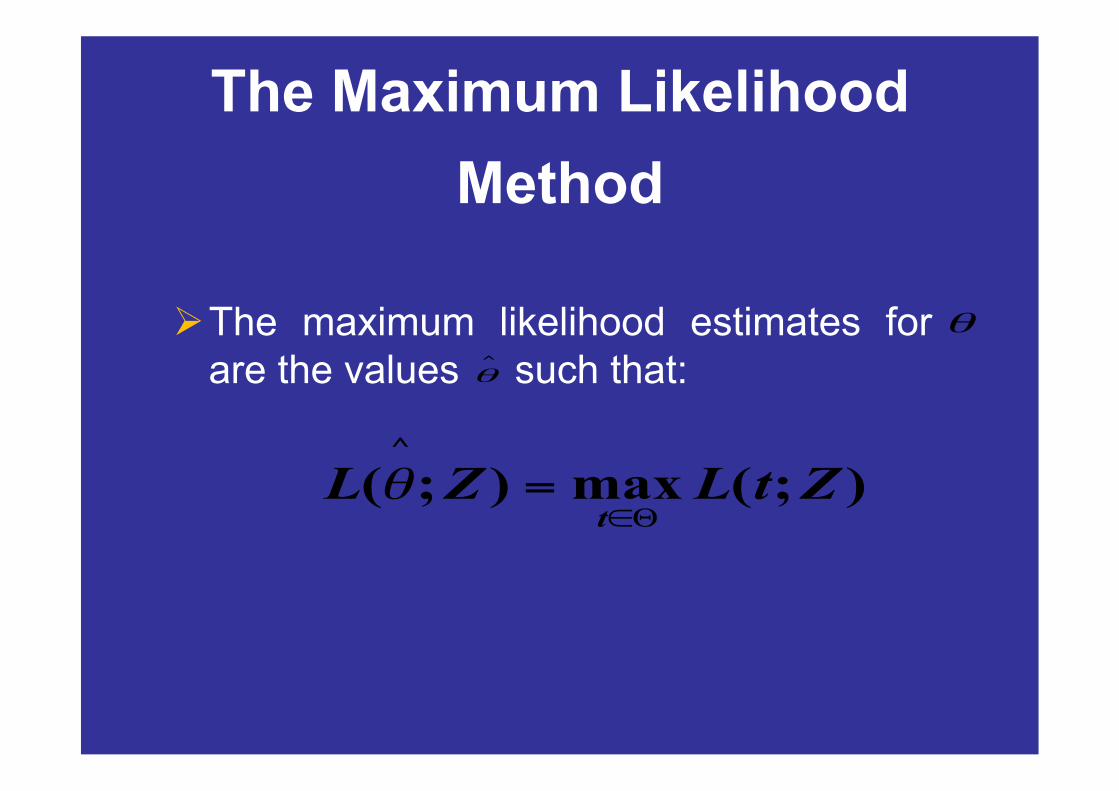
 The maximum likelihood estimates for are the values such that:

The Maximum Likelihood Method

 We are dealing with likelihood functions that are continuous in their parameters, let’s define some differential operators to simplify the notation. For any real valued function a(t), we define D and D2 by:

DERIVATIVE GRADIENT VECTOR

Maximum Likelihood: Commonly used Densities in Micro-

econometrics

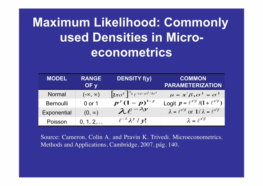
MODEL RANGE OF y

DENSITY f(y) COMMON PARAMETERIZATION

Normal (-∞, ∞) Bernoulli 0 or 1 Logit

Exponential (0, ∞) Poisson 0, 1, 2,…

Source: Cameron, Colin A. and Pravin K. Trivedi. Microeconometrics. Methods and Applications, Cambridge, 2007, pág. 140.

Comparison: Stata and Gauss

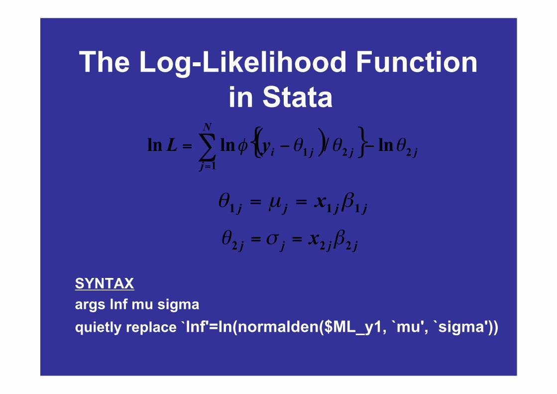
The Log-Likelihood Function in Stata

SYNTAX args lnf mu sigma quietly replace `lnf'=ln(normalden($ML_y1, `mu', `sigma'))

The Log-Likelihood Function in Gauss

Where N is the number of observations, P(Yi, 0) is the probability of Yi given 0, a vector of parameters, and wi is the weight of the i-th observation.

proc loglik(theta,z); local y,x,b,s; x=z[.,1:cols(z)-1]; y=z[.,cols(z)]; b=theta[1:cols(x)]; s=theta[cols(x)+1]; retp(-0.5*ln(s^2)-0.5*(y-x*b)^2/s^2); endp;

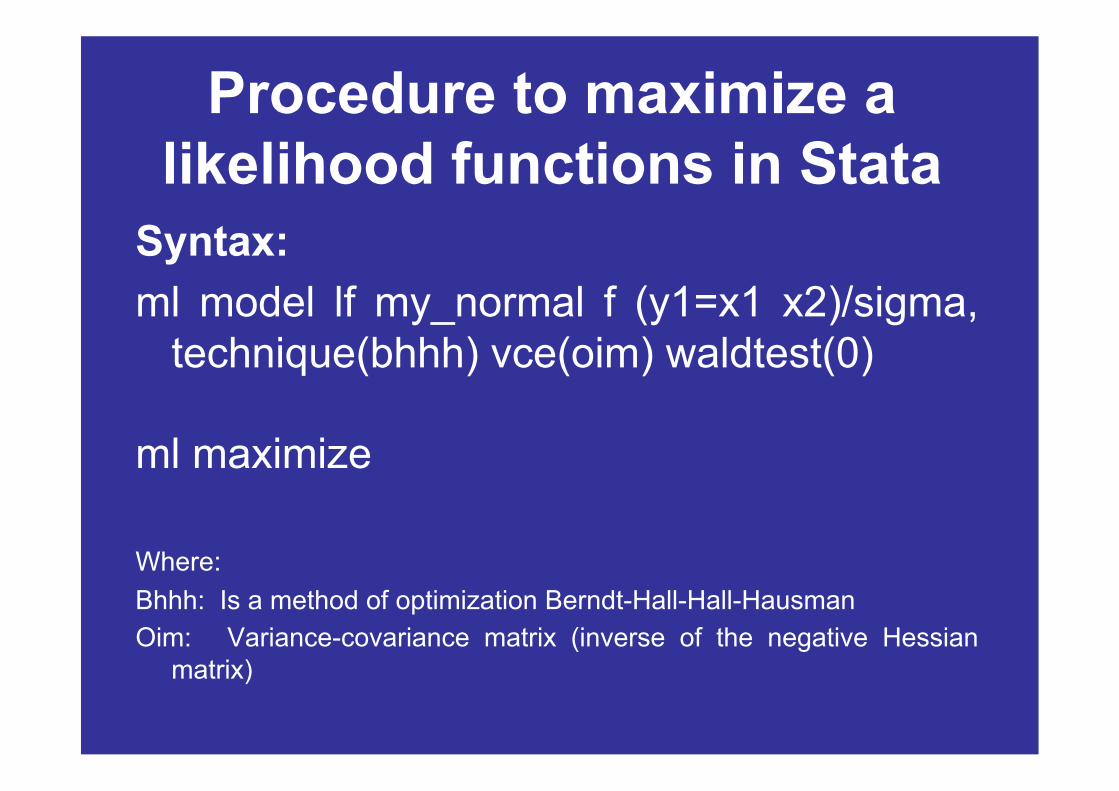
Procedure to maximize a likelihood functions in Stata

Syntax: ml model lf my_normal f (y1=x1 x2)/sigma,

technique(bhhh) vce(oim) waldtest(0)

ml maximize

Where: Bhhh: Is a method of optimization Berndt-Hall-Hall-Hausman Oim: Variance-covariance matrix (inverse of the negative Hessian

matrix)

Procedure to maximize a likelihood functions in Gauss

Capabilities: Stata vs Gauss

 Methods  Optimization Algorithms  Covariance Matrix  Inference Data and Inference  Initial Values  Report of the Coefficients  Other

Stata’s Capabilities: Methods

CAPABILITIES STATA GAUSS

Linear Form Restrictions YES (lnf) NO

No Analytical Derivatives YES (d0) YES

Analytical Gradients First Derivative YES (d1) YES

Analytical Hessian Second Derivative YES (d2) YES

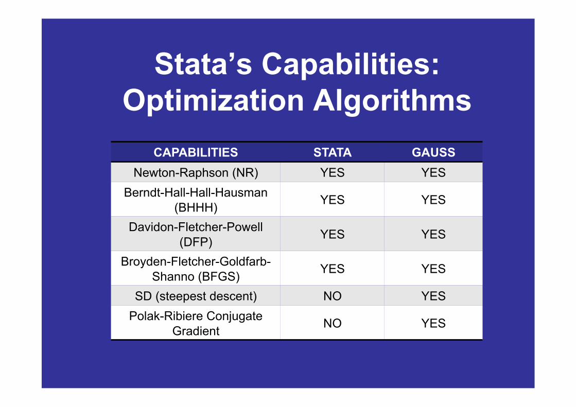
Stata’s Capabilities: Optimization Algorithms

CAPABILITIES STATA GAUSS Newton-Raphson (NR) YES YES

Berndt-Hall-Hall-Hausman (BHHH) YES YES

Davidon-Fletcher-Powell (DFP) YES YES

Broyden-Fletcher-Goldfarb-Shanno (BFGS) YES YES

SD (steepest descent) NO YES Polak-Ribiere Conjugate

Gradient NO YES

Stata’s Capabilities: Covariance Matrix

CAPABILITIES STATA GAUSS

The inverse of the final information matrix from the optimization YES YES

The inverse of the cross-product of the first derivatives YES YES

The hetereskedastic-consistent covariance matrix YES YES

Stata’s Capabilities: Data and Inference

CAPABILITIES STATA GAUSS Robust YES YES Cluster YES NO

Weights* YES YES Survey Data YES (SVY) NO

Modification of the Sub-sample YES NO

Constrains YES NO Wald Test YES YES

Switching** YES YES

* Stata contains frequency, probability, analytic and importance weights. Gauss have only frequency weight. **Switching between algorithms.

Stata’s Capabilities: Initial Values

CAPABILITIES STATA GAUSS

Initial Values YES* YES

Plot YES YES

*Stata searches for feasible initial values with ml search.

Stata’s Capabilities: Report of the Coefficients

CAPABILITIES STATA* GAUSS

Hazard ratios (hr) YES NO

Incidence-rate ratios (irr) YES NO

Odds ratios (or) YES NO

Relative risk ratios (rrr) YES NO

*It must be used the command ml display

Stata’s Capabilities: Other

CAPABILITIES STATA GAUSS

Convergence YES YES

Syntax Errors YES YES

Graph: the log-likelihood values YES YES

Example with the Poisson model ESTIMATION IN STATA ESTIMATION IN GAUSS

program define my_poisson version 9.0 args lnf mu quietly replace `lnf' = $ML y1*ln(`mu')- `mu' - lnfact($ML y1) end

ml model lf my_poisson f (y1=x1 x2)/sigma, technique(bhhh) vce(oim) ml maximize

library maxlik; maxset; proc lpsn(b,z); /* Function - Poisson Regression */

local m; m = z[.,2:4]*b; retp(z[.,1].*m-exp(m)); endp;

proc lgd(b,z); /* Gradient */

retp((z[.,1]-exp(z[.,2:4]*b)).*z[.,2:4]); endp;

x0 = { .5, .5, .5 }; _max_GradProc = &lgd; _max_GradCheckTol = 1e-3; { x,f0,g,h,retcode } = MAXLIK("psn",0,&lpsn,x0); call MAXPrt(x,f0,g,h,retcode);

Conclusions

 Stata’s features seems best suited for analyzing specific models of decision making processes and other micro-econometric applications.

 Gauss is ideal for analyzing a more ample range of statistical issues based on maximum likelihood estimation.