Embed Size (px)
Citation preview
* We thank anonymous referees, Garry Barrett, Ellis Connolly, Ian Halbisch, Geoff Kingston, Grant Turner,Research Group at the Reserve Bank of Australia and participants at the Workshop on the Interactions betweenMicroeconomics and Macroeconomics, National Centre for Econometrics Research, Queensland University ofTechnology and University of New South Wales, the 2009 Conference on Computational Economics, Universityof Technology, Sydney, the 17th Australian Colloquium of Superannuation Researchers, University of New SouthWales and the School of Economics Seminar, Australian National University for comments and assistance. TheChair of Finance and Superannuation (Thorp) is funded by the Sydney Financial Forum (through Colonial FirstState Global Asset Management), the NSW Government, the Association of Superannuation Funds of Australia(ASFA), the Industry Superannuation Network (ISN) and the Paul Woolley Centre for the Study of Capital MarketDysfunctionality within the UTS Business School. We also acknowledge support from ARC DP1093842. Parts ofthe project were completed while Thorp was a visitor at the School of Economics, University of New SouthWales and at the Research Group, Economic Department, Reserve Bank of Australia. This paper uses unit recorddata from the Household, Income and Labour Dynamics in Australia (HILDA) Survey. The HILDA project wasinitiated and is funded by the Australian Government Department of Families, Housing Community Services andIndigenous Affairs (FaHCSIA) and is managed by the Melbourne Institute of Applied Economic and SocialResearch (MIAESR). The findings and views reported in this paper, however, are those of the authors and shouldnot be attributed to either FaHCSIA, MIAESR or the Reserve Bank of Australia.
JEL classifications: D91, E21, G11Correspondence: Susan Thorp, Finance Group, University of Technology, Sydney, P.O. Box 123, Broadway,
THE ECONOMIC RECORD, VOL. 89, NO. 284, MARCH, 2013, 31–51
NSW 2007, Australia. Email: [email protected]
Means-Tested Public Pensions, Portfolio Choice andDecumulation in Retirement*
HARDY HULLEY, REBECCA MCKIBBIN, ANDREAS PEDERSEN and SUSAN THORP
Finance Group, University of Technology, Sydney, New South Wales, Australia
� 2013 The Economdoi: 10.1111/j.1475
Age Pension means-testing buffers retired households againstshocks to wealth and may influence decumulation patterns and port-folio allocations. Simulations from a simple model of optimal con-sumption and allocation strategies for a means-tested retiredhousehold indicate that, relative to benchmark, eligible and near-eligible households should optimally decumulate faster, and choosemore risky portfolios, especially early in retirement. Empiricalmodelling of a Household, Income and Labour Dynamics in Austra-lia panel of pensioner households confirms a riskier portfolio allo-cation by wealthier retired households. Poorer pensionerhouseholds decumulate at around 5 per cent p.a. on average; how-ever, better-off households continue to add around 3 per cent p.a. towealth, even when facing a steeper implicit tax rate on wealth.
31
ic Society of Australia-4932.2012.12002.x
32 ECONOMIC RECORD MARCH
I IntroductionPublic pension systems around the world face
significant pressures as populations age.1
Funded individual accumulations, older retire-ment ages and means-testing of public incometransfers have been proposed as ways to allevi-ate growing demands on government budgets.Here, we investigate the impact of means-testedpublic income transfers on the post-retirementdecumulation and investment behaviour of Aus-tralian retirees. Unlike most other developedeconomies, the Australian retirement incomessystem incorporates a means-testing regime thatextends to around 80 per cent of elderly house-holds, including the wealthiest deciles, and cangive insight into the incentive responsiveness ofrelatively well-off, as well as poorer, households(Harmer, 2008).
The life-cycle model predicts that agents willsave during their working lives and decumulateafter they retire, and that those agents who saveat a faster rate will decumulate more steeply.2
However, empirical evidence for dissaving bythe elderly is inconclusive, with many studies ofcross-sectional and panel data finding that posi-tive or zero saving is common (Borsch-Supan,1992; Alessie et al., 1999; Feinstein & Ho,2000). Among the many reasons offered for thisanomaly is that means-tested public income sup-port may reduce private saving for retirement byeligible and near-eligible households, hencerestricting decumulation after retirement.3 Whileexisting studies show that asset tests can dis-
1 See, for example, Chand and Jaeger (1996), Com-monwealth of Australia (2002), Gruber and Wise(2005), Borsch-Supan et al. (2006) and Novy-Marxand Rauh (2008).
2 See Hurd (1990), Browning and Crossley (2001)and Dynan et al. (2004) for discussion of the life-cycle model as a representation of retirement decumu-lation.
3 Other reasons include precautionary saving foruninsurable medical risks leading to continued accu-mulation later in life, especially among the richretired (Gruber & Yelowitz, 1999; de Nardi et al.,2006); longevity and time preference differences com-pounded by different risk aversion to mortality withthe rich tending to live longer (Hurd, 1990; Hurdet al., 1998); high annuity incomes combining withlater life frailty (Borsch-Supan, 1992; Alessie et al.,1999); unexpectedly high asset returns, which mayappear as persistent savings in short panels; and thedesire to leave a bequest (Hurd, 1990; de Nardi et al.,2006).
courage saving by low-wealth households, theimpact on wealthier households is unclear (Hub-bard et al., 1995; Neumark & Powers, 1998,2000; Ziliak, 2003; Hurst & Ziliak, 2006; deNardi et al., 2006; Sefton et al., 2008).
Recent studies also show that portfolio alloca-tion, as well as overall financial wealth, affectsretirement spending rates. Wachter and Yogo(2010) argue that in the US cross-section, riskyasset exposure increases in wealth but stays fairlystable over the life cycle, whereas Coile andMilligan (2009) show that retired households inthe US tend to reduce holdings of riskier assetclasses in favour of cash deposits in very old age.(Transfers into cash are linked to events whichdecrease wealth, such as the death of a spouse orill-health.) It follows that decumulation may beslower among wealthier households because theycan benefit from risk premia. Furthermore, ifpoorer retirees tend to be heavily invested in thefamily home, they have less access to liquid con-sumable wealth than is indicated by their relativenet worth (Sinai & Souleles, 2007). Finally, vol-untary annuitisation of retirement accumulationsmay be crowded out by means-tested pensions ashouseholds may cash out occupational accumula-tions while preserving their public payments(Butler et al., 2011). Means tests may alsoencourage risk exposure by dynamically hedgingincome against negative financial shocks, as wediscuss below.
Here, we study the decumulation pattern ofAustralian Age Pensioners over the period 2002–2006. The unique structure of the Australianretirement savings system (outlined in Section I),with its broadly targeted basic pension and lim-ited use of annuitisation, can give insight into theincentives of means-testing on retirees across thewealth distribution. Moreover, we can considerthe impact of portfolio composition on decumula-tion patterns. In Section II, using a standard con-stant relative risk aversion (CRRA) utilityframework and uncertain investment returns, wesolve the dynamic consumption and portfolioallocation problem of the means-tested retiredhousehold.4 Simulations predict that the prospect
4 We recognise that pre-retirement decisions arealmost surely influenced by the pension regulations,but our panel of wealth data is restricted to eligiblehouseholds over the age of 65, so we limit our studyto the behaviour of that group. Moreover, we restrictour sample to 2006 to avoid regulation changes afterthat date.
� 2013 The Economic Society of Australia
5 By income measures, most pensioners are lesswell-off, with the large majority in the lowest incomequartile, but more than 2 per cent (around 50,000) arein the highest quartile (Kelly, 2009).
6 Details of payments and eligibility are at http://www.humanservices.gov.au/customer/services/centre-link/age-pension.
2013 MEANS-TESTED PUBLIC PENSIONS 33
of receiving a low-risk, means-tested incomepayment is likely to encourage rapid drawdownearly in retirement by wealthier households.However, the wealth-hedging properties of themeans tests motivate a risky asset exposure thatis optimally higher and more variable than thebenchmark case and may generate higher retire-ment incomes.
We evaluate these predictions using anannual series for the approximate net wealthof Age Pensioner households from the House-hold Income and Labour Dynamics (HILDA)panel. (Section III profiles Age Pensionerwealth from HILDA 2006 to create a referencepoint for panel estimation.) The HILDA sur-vey does not collect wealth information ateach wave, but we can make use of pensionregulations and reported Age Pension receiptsto infer annual net worth over 2002–2006. Weestimate annual dissaving rates for groups ofhouseholds that are subject to different meanstests, and differentiated by bequest and pre-cautionary savings motives (Section IV).Section V concludes.
II Means-Tested Pension Payments in AustraliaUnlike the USA and the UK, which offer
earnings-linked social security payments, theAustralian public pension does not pay out onthe basis of wage history. It creates a safety netand supplements mandatory (SuperannuationGuarantee) and voluntary individual accumula-tions. While dependence on the public pensionis expected to ease as the Superannuation Guar-antee system matures, the Australian Govern-ment estimates that around 60 per cent ofelderly households will still receive a full orpart Age Pension payment by the middle of thiscentury. Consequently, pension means tests willinteract with population ageing causing the fis-cal burden to rise (Commonwealth of Australia,2002).
Currently, most retired Australians qualify forsome income support with around 77 per cent ofindividuals over the age of 65 (2 million people)receiving all or part of the Age Pension (Har-mer, 2008). Eligibility depends on age and resi-dency status, and payments are tested overcurrent income and assets. The family home isexcluded from the asset test, but all other realand financial assets are assessed, including per-sonal effects and home contents. Despite meanstesting, most wealthy retired households receivea part pension: almost 50 per cent of eligible
� 2013 The Economic Society of Australia
households are in the top half of the nationalwealth distribution, and close to 14 per cent arein the top wealth quartile.5 The effectiveness ofthe Age Pension as an income supplement andsafety net will depend on both the total amounttransferred and on how efficiently transfers aredistributed among eligible households.
A single pensioner who owns their own homeis paid around 28 per cent of Male Total Aver-age Weekly Earnings (MTAWE) and partneredpensioners receive 75.5 per cent of the singlepayment each.6 Compared with other OECDcountries, the Age Pension creates low replace-ment rates (Harmer, 2008), but eligibility ishighly valued: generating a similar stream ofincome from private savings via commercialincome stream products would require an accu-mulation of around seven times average annualincomes (Petrichev & Thorp, 2008). The basesingle pension is recalculated every 6 months(March and September) to keep up with changesin the Consumer Price Index (CPI) or the Pen-sioner and Beneficiaries Living Cost Index(PBLCI) and also to ensure that it does not fallbelow 25 per cent of MTAWE. Pensionerstherefore hold an option on the general level ofwages and prices in the economy, and over thepast decade, the real pension payment hasincreased by around 2 per cent per year, whichhas been sufficient to maintain or improve rela-tivity with low-income working households(Harmer, 2008).
Means tests begin to reduce the pension atfixed nominal levels of income and/or assets andboundaries are revised with changes in prices.As the means tests may interact with each other,the pensioner is entitled to the least paymentfrom either test or zero. The means test bound-aries and taper rates are adjusted frequently, soin the discussion below, we look at the means-test rules applying in 2006 (to approximate ourpanel sample).
Under the income test, individuals can receivearound 25 per cent of the base pension payment
34 ECONOMIC RECORD MARCH
in private income before payments begin todecrease at $0.40 for each additional dollarearned.7 Under the assets test, the pensionincreases by $78 p.a. per $1000 decrease inassessable wealth Vt, from the upper asset bound-ary A2 (see Table 1) until the lower boundary atA1.8 In addition, on becoming eligible for anypension payment, retirees received allowancestowards the cost of pharmaceuticals, utilities, etc,which have since been largely replaced by a fixedpension supplement. This step in payments wasworth around $300 p.a. for most pensioners overthe time we study and we denote it C0.
As many retirees rely entirely on financialassets for all extra income, regulators ‘deem’fixed rates of return for income from financialassets rather than relying on individuals to esti-mate investment returns for the year ahead, or tomake adjustments after returns are realised. In2006, for example, financial assets up to a valueof $38,400 were deemed to accrue income at a rateof 3 per cent p.a. and for all financial assets abovethat value, income was deemed to accrue at 5 percent p.a. The deeming rules allow us to translatethe income test boundaries into an equivalentwealth test (Y1 and Y2) by assuming that allincome comes from financial asset returns.Table 1 details the means-tests limits for a single,home-owner pensioner that applied in 2006.9
The income test binds earlier than the assetstest, at V ¼ Y1, but the assets test begins to bindat the point of intersection between the two
lines VI ¼ A2ðY1�Y2Þ�Y2ðA1�A2ÞðY1�Y2Þ�ðA1�A2Þ , and becomes the
binding constraint until P(t) ¼ 0, at V ¼ A2.
7 Changes since 2008 mean that payments nowdecrease at 50 cents for each additional dollar ofincome with an additional free allowance of $500 forlabour income.
8 In 2007, the asset taper was decreased to $39 perthousand dollars of wealth.
9 Most retirement accumulations in Australia aretaken as lump sums and invested outside the Superan-nuation system. However, approximately 40 per centare used to purchase income streams. Income receivedfrom retirement income streams such as annuities andallocated pensions is means-tested under formulasdesigned to separate capital drawdown from invest-ment earnings. Annuity income is difficult to identifyseparately in our data, and the assessment formulashave been changed several times over the course ofthe sample. We approximate the wealth value of annu-ities by the same method as for other income fromother financial assets.
Combining the two constraints gives us the cur-rent pension payment as a function of wealth atthe beginning of period t, P(Vt),
PðVtÞ ¼
P0 þC0�P0Y2Y1�Y2þ
P0Y1�Y2 Vt þC0
�P0A2A1�A2þ
P0A1�A2 Vt þC0
0
8>>><>>>:
if Vt � Y1
if Y1< Vt � VI
if VI < Vt � A2
if A2< Vt
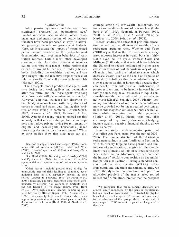
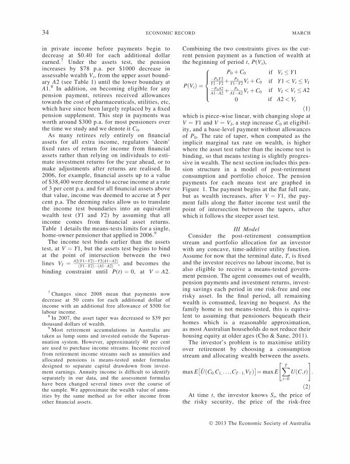
ð1Þwhich is piece-wise linear, with changing slope atV ¼ Y1 and V ¼ VI, a step increase C0 at eligibil-ity, and a base-level payment without allowancesof P0. The rate of taper, when computed as theimplicit marginal tax rate on wealth, is higherwhere the asset test rather than the income test isbinding, so that means testing is slightly progres-sive in wealth. The next section includes this pen-sion structure in a model of post-retirementconsumption and portfolio choice. The pensionpayments for each means test are graphed inFigure 1. The payment begins at the flat full rate,but as wealth increases, after V ¼ Y1, the pay-ment falls along the flatter income test until thepoint of intersection between the tapers, afterwhich it follows the steeper asset test.
III ModelConsider the post-retirement consumption
stream and portfolio allocation for an investorwith any concave, time-additive utility function.Assume for now that the terminal date, T, is fixedand the investor receives no labour income, but isalso eligible to receive a means-tested govern-ment pension. The agent consumes out of wealth,pension payments and investment returns, invest-ing savings each period in one risk-free and onerisky asset. In the final period, all remainingwealth is consumed, leaving no bequest. As thefamily home is not means-tested, this is equiva-lent to assuming that pensioners bequeath theirhomes which is a reasonable approximation,as most Australian households do not reduce theirhousing equity at older ages (Cho & Sane, 2011).
The investor’s problem is to maximise utilityover retirement by choosing a consumptionstream and allocating wealth between the assets.
max E UðC0;C1; . . .;CT�1;VTÞ� �
¼max EXT
t¼0
UðC;tÞ" #
:
ð2ÞAt time t, the investor knows St, the price of
the risky security, the price of the risk-free
� 2013 The Economic Society of Australia
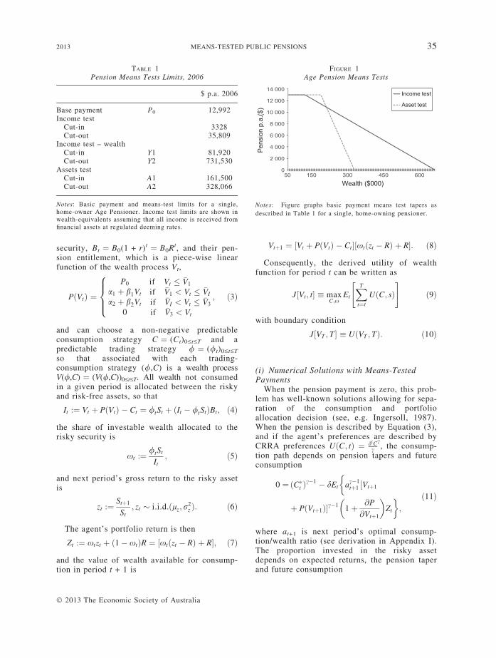
TABLE 1Pension Means Tests Limits, 2006
$ p.a. 2006
Base payment P0 12,992Income test
Cut-in 3328Cut-out 35,809
Income test – wealthCut-in Y1 81,920Cut-out Y2 731,530
Assets testCut-in A1 161,500Cut-out A2 328,066
Notes: Basic payment and means-test limits for a single,home-owner Age Pensioner. Income test limits are shown inwealth-equivalents assuming that all income is received fromfinancial assets at regulated deeming rates.
Wealth ($000)
Pen
sion
p.a
.($)
Income test
Asset test
FIGURE 1Age Pension Means Tests
Notes: Figure graphs basic payment means test tapers as
described in Table 1 for a single, home-owning pensioner.
2013 MEANS-TESTED PUBLIC PENSIONS 35
security, Bt ¼ B0(1 + r)t ¼ B0Rt, and their pen-sion entitlement, which is a piece-wise linearfunction of the wealth process Vt,
PðVtÞ ¼
P0
a1 þ b1Vt
a2 þ b2Vt
0
8>><>>:
if Vt � �V1
if �V1 < Vt � �VI
if �VI < Vt � �V3
if �V3 < Vt
; ð3Þ
and can choose a non-negative predictableconsumption strategy C ¼ (Ct)0£t£T and apredictable trading strategy / ¼ (/t)0£t£T
so that associated with each trading-consumption strategy (/,C) is a wealth processV(/,C) ¼ (V(/,C))0£t£T. All wealth not consumedin a given period is allocated between the riskyand risk-free assets, so that
It :¼ Vt þ PðVtÞ � Ct ¼ /tSt þ ðIt � /tStÞBt; ð4Þ
the share of investable wealth allocated to therisky security is
xt :¼ /tSt
It; ð5Þ
and next period’s gross return to the risky assetis
zt :¼ Stþ1
St; zt � i.i.d.ðlz; r
2z Þ: ð6Þ
The agent’s portfolio return is then
Zt :¼ xtzt þ ð1� xtÞR ¼ ½xtðzt � RÞ þ R�; ð7Þ
and the value of wealth available for consump-tion in period t + 1 is
� 2013 The Economic Society of Australia
Vtþ1 ¼ ½Vt þ PðVtÞ � Ct�½xtðzt � RÞ þ R�: ð8Þ
Consequently, the derived utility of wealthfunction for period t can be written as
J½Vt; t� � maxC;x
Et
XT
s¼t
UðC; sÞ" #
ð9Þ
with boundary condition
J½VT ; T� � UðVT ; TÞ: ð10Þ
(i) Numerical Solutions with Means-TestedPayments
When the pension payment is zero, this prob-lem has well-known solutions allowing for sepa-ration of the consumption and portfolioallocation decision (see, e.g. Ingersoll, 1987).When the pension is described by Equation (3),and if the agent’s preferences are described byCRRA preferences UðC; tÞ ¼ dtC
c
c, the consump-
tion path depends on pension tapers and futureconsumption
0 ¼ðC�t Þc�1 � dEt
�ac�1
tþ1 ½Vtþ1
þ PðVtþ1Þ�c�1 1þ @P
@Vtþ1
� �Zt
�;
ð11Þ
where at+1 is next period’s optimal consump-tion/wealth ratio (see derivation in Appendix I).The proportion invested in the risky assetdepends on expected returns, the pension taperand future consumption
36 ECONOMIC RECORD MARCH
Et ac�1tþ1 ½Vtþ1þPðVtþ1Þ�c�1 1þ @P
@Vtþ1
� �ðzt�RÞ
� �¼0:
ð12Þ
As the value function is unknown, analyticalsolutions are not available, and we use numeri-cal methods. We establish a grid of values forwealth, the state variable, in each period, andsearch for optimal consumption and risky assetinvestment proportions at each point in the gridin each period. Using Gaussian Quadrature tocompute the value function for a given con-sumption and investment strategy, we then usenumerical optimisation to maximise the valuefunction across all consumption and investmentstrategies at each point on the grid, and theninterpolate to construct an approximate repre-sentation of the value function.
(ii) ParameterisationWe simulate the model to give a flavour of
how the pension causes the time path of controlsto vary from the standard case, rather than toclosely match observed paths. Simulationsassume preferences are described by log utilityand that model parameters are fixed and knownwith certainty. Rates of relative risk aversionclose to one are supported by micro studies oflife-cycle consumption behaviour (Attanasioet al., 1999; Gourinchas & Parker, 2002).The real annual risk-free rate of return is set at
Ag
Con
sum
ptio
n p.
a ($
)
FIGURE
Simulated Consu
Notes: Figure graphs simulated consumption paths over 20 years
preferences, and assuming that the risky asset pays expected return
regulations are set out in Table 1.
R ¼ 1.03, the return to the risky asset atE(z) ¼ lz¼el ¼ 1.0408 with a standard devia-tion, SD[z]¼el(er2
)1)1/2¼ 0.21. This unusuallylow equity premium allows for interior solutionsto the portfolio allocation path. (In simulation,we constrain the risky asset exposure / to the[0,1] interval to reflect the borrowing constraintsof the elderly. As risk aversion is low, the opti-mal solution is at the boundary for higher equitypremia.) We set the subjective discount factor to0.97 for the purposes of illustration, althoughmuch higher and more variable rates are sup-ported by some studies (Attanasio et al., 1999;Alan & Browning, 2006). The means-tests con-straints used in the simulation are set out inTable 1. We compare the simulated results witha benchmark case where no public pension ispaid and the individual manages their retirementwealth according to the optimisation modeldescribed above.
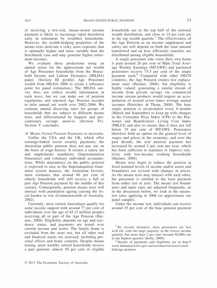
(iii) Simulation Results and DiscussionFigure 2 graphs the optimal consumption path
and consumption-to-wealth ratio over a 20-yearhorizon, assuming that the risky asset pays itsexpected return in each year and initial financialwealth is $500,000. The dotted line is optimalconsumption under the 2006 pension rules, whenthe overall value of the payment was close to$13,000. Consumption increases until wealthreaches the cut-out level for the asset test, A2,
e
Con
sum
ptio
n/w
ealth
2mption Paths
for single retiree with initial wealth of $500,000, log utility
in each year. The constant discount rate is 0.97 p.a. Pension
� 2013 The Economic Society of Australia
Income test
Assets test
Full pension
Age
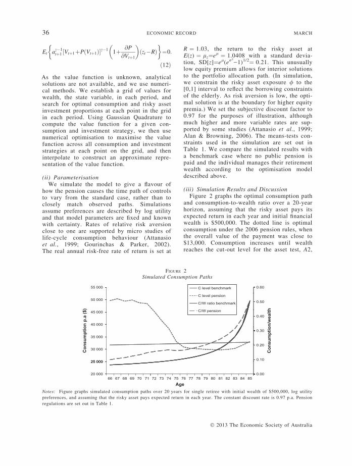
FIGURE 3Spending Rates Under Asset and Income Tapers
Notes: Figure graphs simulated optimal dissaving ratios over 20 years for single retiree at different initial wealth levels, log util-
ity preferences, and assuming that the risky asset pays its expected return in each year. The constant discount rate is 0.97 p.a.
Pension regulations are set out in Table 1.
10 Tax concessions continue to apply to accumula-tions kept in superannuation accounts after retirement,but regulations control spending rates to minimumannual levels which vary with age (see Bateman &Thorp, 2008).
2013 MEANS-TESTED PUBLIC PENSIONS 37
around age 71, then declines over the steepertaper to the point of intersection between theincome and asset tapers, VI, around age 75, thenflattens over the gentler taper. The means testscreate incentives to reduce early-retirementwealth at a faster rate than is optimal under theno-pension benchmark (solid line). The con-sumption-to-wealth ratio is higher over thewhole of retirement under the means-tested pay-ment, even at times when the actual amountbeing contributed by the pension is relativelysmall.
Figure 3 shows the impact of the tapers ondrawdown rates from another perspective. Con-sider how the means tests apply as wealthdecreases along the horizontal axis of Figure 1:the steeper assets test taper applies when wealthis around $330,000, the flatter income taperapplies from $188,000, and the maximumamount of pension is always paid when wealthfalls below $82,000. If we set initial wealthclose to each of these levels, optimal drawdownrates follow different paths. The wealthiesthousehold (V(0) ¼ $300,000) is subject to thefaster taper and draws down steeply (6 per cent)early in retirement, then gradually decreasesthat rate to around 2 per cent, finally increasingthe spending rate near the terminal date. Thehousehold on the flatter income taper (V(0) ¼$190,000) begins to draw down at 2 per centp.a., consuming faster than the householdreceiving the full pension and not subject to any
� 2013 The Economic Society of Australia
taper (V(0) ¼ $100,000), but much less quicklythan the richer household. In effect, implicit taxrates encourage different rates of wealth reduc-tion by all households depending on their accu-mulation at retirement, whereas the rate ofchange in wealth under the no-pension bench-mark is the same at all initial savings levels.
Few studies have looked into the impact ofpension streams on portfolio allocation. This isa particularly interesting question for Australianretirees, the majority of whom do not annuitiseat retirement but continue to hold individualinvestment accounts both inside and outside thesuperannuation system,10 and the issue hasinternational significance for pension regulatorswho are overseeing the transition to individualaccounts from public- or private-defined bene-fit pension schemes. The Age Pension is alow-volatility real annuity stream with a payoffthat is negatively correlated with the risky assetbecause of the means tests. Pension entitlementtherefore creates a substitute for the risk-freeasset, a hedge against other risks to wealth,encourages higher risk exposure by beneficia-ries, and transfers risk from individuals to the
Age
Port
folio
wei
ght
Benchmark
Pension
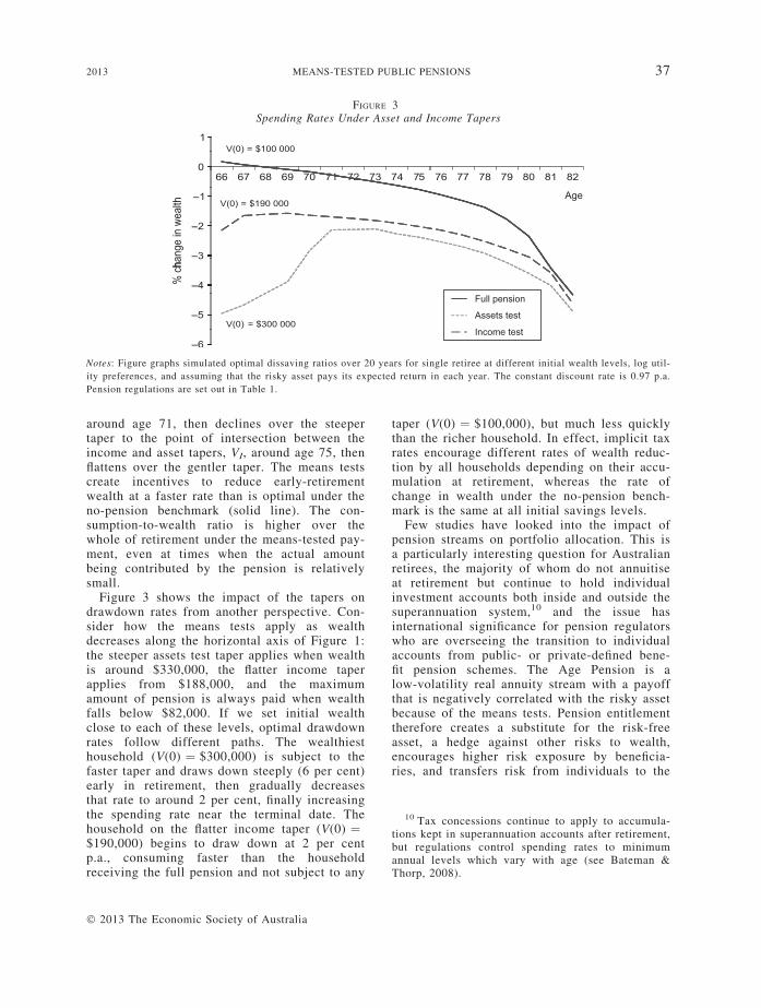
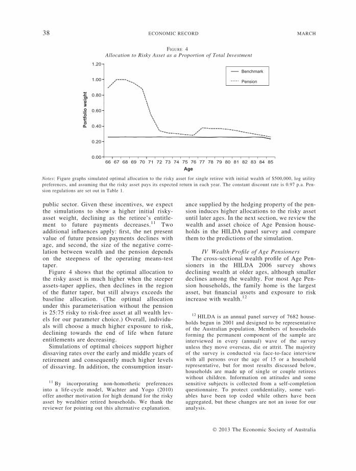
FIGURE 4Allocation to Risky Asset as a Proportion of Total Investment
Notes: Figure graphs simulated optimal allocation to the risky asset for single retiree with initial wealth of $500,000, log utility
preferences, and assuming that the risky asset pays its expected return in each year. The constant discount rate is 0.97 p.a. Pen-
sion regulations are set out in Table 1.
12 HILDA is an annual panel survey of 7682 house-holds begun in 2001 and designed to be representativeof the Australian population. Members of householdsforming the permanent component of the sample areinterviewed in every (annual) wave of the surveyunless they move overseas, die or attrit. The majorityof the survey is conducted via face-to-face interviewwith all persons over the age of 15 or a householdrepresentative, but for most results discussed below,
38 ECONOMIC RECORD MARCH
public sector. Given these incentives, we expectthe simulations to show a higher initial risky-asset weight, declining as the retiree’s entitle-ment to future payments decreases.11 Twoadditional influences apply: first, the net presentvalue of future pension payments declines withage, and second, the size of the negative corre-lation between wealth and the pension dependson the steepness of the operating means-testtaper.
Figure 4 shows that the optimal allocation tothe risky asset is much higher when the steeperassets-taper applies, then declines in the regionof the flatter taper, but still always exceeds thebaseline allocation. (The optimal allocationunder this parameterisation without the pensionis 25:75 risky to risk-free asset at all wealth lev-els for our parameter choice.) Overall, individu-als will choose a much higher exposure to risk,declining towards the end of life when futureentitlements are decreasing.
Simulations of optimal choices support higherdissaving rates over the early and middle years ofretirement and consequently much higher levelsof dissaving. In addition, the consumption insur-
11 By incorporating non-homothetic preferencesinto a life-cycle model, Wachter and Yogo (2010)offer another motivation for high demand for the riskyasset by wealthier retired households. We thank thereviewer for pointing out this alternative explanation.
ance supplied by the hedging property of the pen-sion induces higher allocations to the risky assetuntil later ages. In the next section, we review thewealth and asset choice of Age Pension house-holds in the HILDA panel survey and comparethem to the predictions of the simulation.
IV Wealth Profile of Age PensionersThe cross-sectional wealth profile of Age Pen-
sioners in the HILDA 2006 survey showsdeclining wealth at older ages, although smallerdeclines among the wealthy. For most Age Pen-sion households, the family home is the largestasset, but financial assets and exposure to riskincrease with wealth.12
households are made up of single or couple retireeswithout children. Information on attitudes and somesensitive subjects is collected from a self-completionquestionnaire. To protect confidentiality, some vari-ables have been top coded while others have beenaggregated, but these changes are not an issue for ouranalysis.
� 2013 The Economic Society of Australia
Percentile
Mea
n as
sets
($)
Mea
n fin
anci
al a
sset
s ($
)
Percentile
(a) (b)
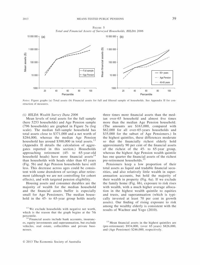
FIGURE 5Total and Financial Assets of Surveyed Households, HILDA 2006
Notes: Figure graphs (a) Total assets (b) Financial assets for full and filtered sample of households. See Appendix II for con-
struction of measures.
2013 MEANS-TESTED PUBLIC PENSIONS 39
(i) HILDA Wealth Survey Data 2006Mean levels of total assets for the full sample
(here 5253 households) and Age Pension sample(796 households) are graphed in Figure 5a (logscale). The median full-sample household hastotal assets close to $371,000 and a net worth of$284,000, whereas the median Age Pensionhousehold has around $300,000 in total assets.13
(Appendix II details the calculation of aggre-gates reported in this section.) Householdsapproaching retirement (45- to 65-year-oldhousehold heads) have more financial assets14
than households with heads older than 65 years(Fig. 5b) and Age Pension households have stillless. This decrease across ages could be consis-tent with some drawdown of savings after retire-ment (although we are not controlling for cohorteffects), and with targeted pension eligibility.
Housing assets and consumer durables are themajority of wealth for the median householdand the financial assets buffer is especiallysmall for Age Pensioners. The median house-hold in the 45- to 65-year group holds nearly
13 We exclude households with negative net worth,which is the reason that the graph begins at the 7thpercentile.
14 Financial assets include bank accounts, insuranc-es, equity investments and superannuation, but excludevehicles, real estate, collectibles and private busi-nesses.
� 2013 The Economic Society of Australia
three times more financial assets than the med-ian over-65 household and almost five timesmore than the median Age Pension household.(The amounts are $163,000, compared with$62,000 for all over-65-years households and$35,000 for the subset of Age Pensioners.) Inthe highest quintiles, these differences moderateso that the financially richest elderly holdapproximately 90 per cent of the financial assetsof the richest of the 45- to 65-year group,whereas the highest Age Pension wealth quintilehas one quarter the financial assets of the richestpre-retirement households.15
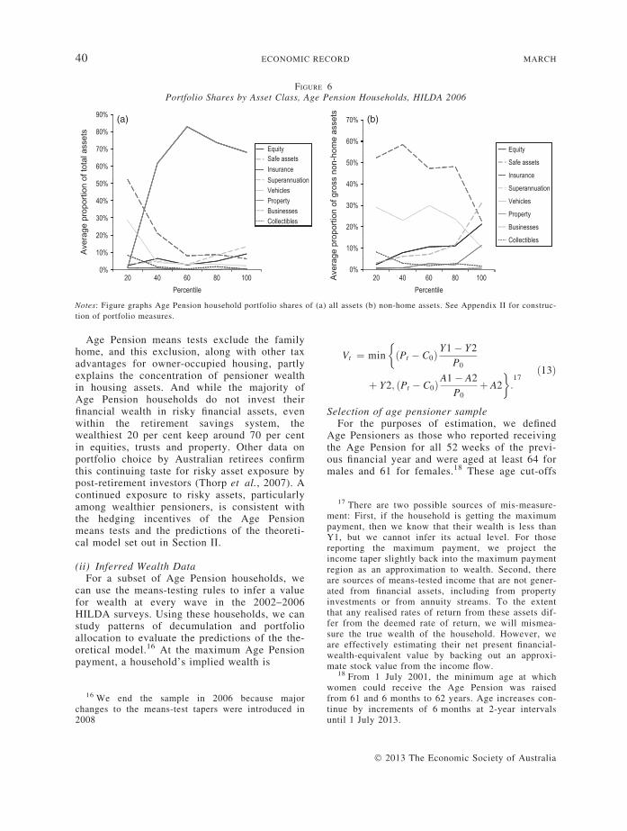
Pensioners keep a low proportion of theirtotal assets as liquid and tradable financial secu-rities, and also relatively little wealth in super-annuation accounts, but hold the majority oftheir wealth in property (Fig. 6a). If we excludethe family home (Fig. 6b), exposure to risk riseswith wealth, with a much higher average alloca-tion in the highest wealth quintile to equitiesand trusts, and superannuation (which is typi-cally invested at least 70 per cent in growthassets). Our finding of rising exposure to riskamong the wealthy elderly is consistent with theresults of Wachter and Yogo (2010).
15 Mean financial assets in the highest quintiles are(pre-retirement) $934,000, (over 65 years) $826,000,and (Age Pensioner) $246,000, respectively.
Percentile
Ave
rage
pro
porti
on o
f tot
al a
sset
s
Ave
rage
pro
porti
on o
f gro
ss n
on-h
ome
asse
ts
Percentile
EquitySafe assetsInsuranceSuperannuationVehiclesPropertyBusinessesCollectibles
Equity
Safe assets
Insurance
Superannuation
Vehicles
Property
Businesses
Collectibles
(a) (b)
FIGURE 6Portfolio Shares by Asset Class, Age Pension Households, HILDA 2006
Notes: Figure graphs Age Pension household portfolio shares of (a) all assets (b) non-home assets. See Appendix II for construc-
tion of portfolio measures.
17 There are two possible sources of mis-measure-ment: First, if the household is getting the maximumpayment, then we know that their wealth is less thanY1, but we cannot infer its actual level. For thosereporting the maximum payment, we project theincome taper slightly back into the maximum paymentregion as an approximation to wealth. Second, thereare sources of means-tested income that are not gener-ated from financial assets, including from propertyinvestments or from annuity streams. To the extentthat any realised rates of return from these assets dif-fer from the deemed rate of return, we will mismea-sure the true wealth of the household. However, weare effectively estimating their net present financial-wealth-equivalent value by backing out an approxi-mate stock value from the income flow.
40 ECONOMIC RECORD MARCH
Age Pension means tests exclude the familyhome, and this exclusion, along with other taxadvantages for owner-occupied housing, partlyexplains the concentration of pensioner wealthin housing assets. And while the majority ofAge Pension households do not invest theirfinancial wealth in risky financial assets, evenwithin the retirement savings system, thewealthiest 20 per cent keep around 70 per centin equities, trusts and property. Other data onportfolio choice by Australian retirees confirmthis continuing taste for risky asset exposure bypost-retirement investors (Thorp et al., 2007). Acontinued exposure to risky assets, particularlyamong wealthier pensioners, is consistent withthe hedging incentives of the Age Pensionmeans tests and the predictions of the theoreti-cal model set out in Section II.
(ii) Inferred Wealth DataFor a subset of Age Pension households, we
can use the means-testing rules to infer a valuefor wealth at every wave in the 2002–2006HILDA surveys. Using these households, we canstudy patterns of decumulation and portfolioallocation to evaluate the predictions of the the-oretical model.16 At the maximum Age Pensionpayment, a household’s implied wealth is
16 We end the sample in 2006 because majorchanges to the means-test tapers were introduced in2008
Vt ¼ min
�ðPt � C0Þ
Y1� Y2P0
þ Y2; ðPt � C0ÞA1� A2
P0þ A2
�:17
ð13Þ
Selection of age pensioner sampleFor the purposes of estimation, we defined
Age Pensioners as those who reported receivingthe Age Pension for all 52 weeks of the previ-ous financial year and were aged at least 64 formales and 61 for females.18 These age cut-offs
18 From 1 July 2001, the minimum age at whichwomen could receive the Age Pension was raisedfrom 61 and 6 months to 62 years. Age increases con-tinue by increments of 6 months at 2-year intervalsuntil 1 July 2013.
� 2013 The Economic Society of Australia
20 Age Pension recipients are also eligible for sev-eral supplement payments; however, the HILDA sur-vey questions do not ask specifically about thesepayments. It is therefore unclear whether or not
2013 MEANS-TESTED PUBLIC PENSIONS 41
were supported by the data. By using an annualpension payment, we exclude people who didnot receive the Age Pension for a full year.19
There were 1915 individuals living in 1529households that met this criteria, but a series offurther exclusions are needed, based on house-hold structure, homeownership and retirementstatus.
We select samples of single and couplehouseholds, excluding 360 individuals living in300 households that are of a different type, asthe rate of pension payment may vary whenother people are included in the household andour method does not allow for this. We furtherlimit the sample to home owners because thoserenting are eligible for additional payments,which are not itemised in the HILDA Survey.There are a further 429 individuals and 363households that are excluded because they arenot home owners. Finally, we focus on peoplewho are retired and earning income largely fromasset returns.
Retirement is difficult to capture because therelevant questions do not appear in the sameform in every wave of the HILDA survey. Anal-ysis of the data also suggested that people havedifferent subjective definitions of retirement;some people who perform a small amount ofunpaid voluntary work consider themselves tonot be retired, while others who only work part-time do consider themselves to be retired. Thisis further confused by the fact that people whohave been out of the labour force for a long per-iod of time, mostly women, may not considerthemselves to be retired, but we want to includethem in the sample as they are effectivelyretired. We constructed the retirement measureby cross-checking the labour force calendaractivity with reported retirement, householdform eligibility for labour force questions andfinancial year income from wages and salaryand own business. There are 266 Age Pensionersliving in 248 households who are not fullyretired based on our measure.
For couple households we only include thehouseholds if both individuals meet the retiredAge Pensioner criteria, as couples are assessedjointly for the purposes of social security pay-ments. There are 363 individuals in 307 couple
19 People who received a full pension for part ofthe year will appear to be more wealthy than theyactually are.
� 2013 The Economic Society of Australia
households who do not meet this restriction.These leave a final sample of 837 households(368 couples and 469 singles) with a total of2631 observations. In the analysis, we removed7 singles because they were couples in the pre-vious period who have separated or where onepartner has passed away. We also remove 22households who do report the total amount oftheir pension and take out 109 singles and 93couples households because they either did nothave two consecutive observations to allow theasset drawdown variable to be calculated ortheir reported pension was more than 10 percent above the maximum rate. The final sampleis 346 singles and 264 couples, with a totalnumber of observations of 935 observations onsingles and 712 couples.
The majority of the Age Pensioners in oursub-sample are single and of low education,their median age is 74 years, and more than 65per cent are female, characteristics matching uppretty well to the whole population of pension-ers (Harmer, 2008). A large minority report fairor poor health (Table 2).
There are two measures of the amount of AgePension received available in HILDA – theamount received in the previous financial year(either in total or the average fortnightlyamount) and the current fortnightly rate. Theprevious financial year measure, annualised, isthe best measure for our calculation of impliedwealth because the most recently received pay-ment may be influenced by short-term fluctua-tions in income or wealth. As the pension ratesand means-testing parameters change during theyear, a weighted average for the financial yearwas constructed for the calculation.20 However,after doing this, we found that over a third ofthe sample reported a pension rate that wasabove the maximum possible rate. Moreover,71.6 per cent of the 80.9 per cent of people whoreported an average weekly pension rate gavethe same rate for the previous financial year andthe current rate received. While this is techni-
respondents would have included these amounts intheir reporting. It is assumed that they are included inthe reporting of the Age Pension because a large pro-portion of people report an amount above the maxi-mum possible payment.
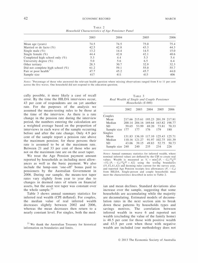
TABLE 2Household Characteristics of Age Pensioner Panel
2003 2004 2005 2006
Mean age (years) 74.5 74.5 75.0 75.4Married or de facto (%) 42.5 42.8 43.3 44.3Single male (%) 13.2 14.4 14.5 15.0Single female (%) 44.4 42.8 42.1 40.6Completed high school only (%) 5.3 4.4 5.3 5.4University degree (%) 5.0 5.6 6.5 6.4Other tertiary 28.3 30.7 32.9 32.3Did not complete high school (%) 61.2 59.1 55.0 55.7Fair or poor health† 47.7 45.2 45.7 44.0Sample size 417 411 413 406
Notes: †Percentage of those who answered the relevant health question where missing observations ranged from 8 to 11 per centacross the five waves. One household did not respond to the education question.
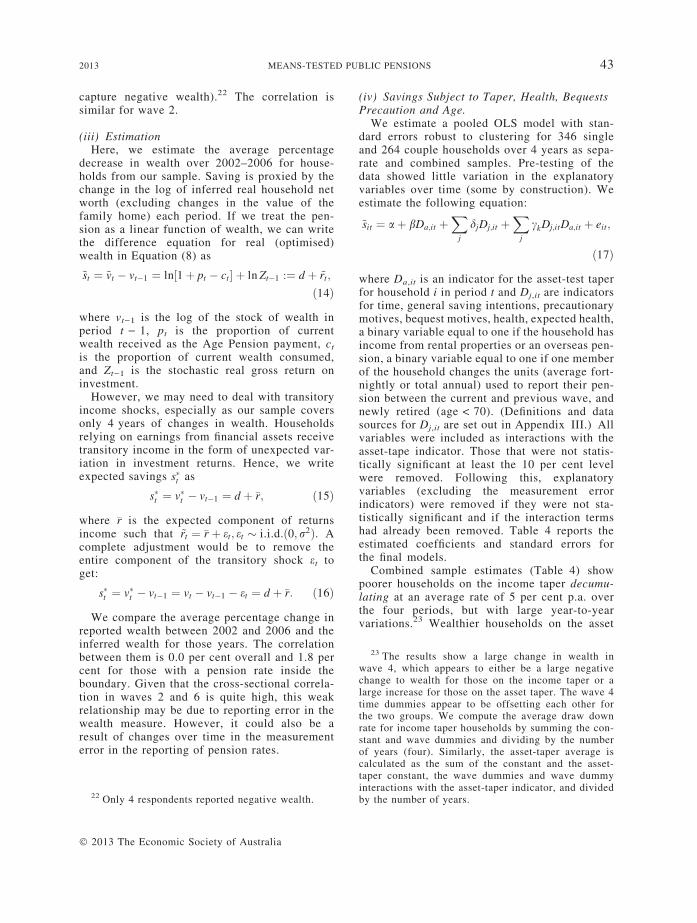
TABLE 3Real Wealth of Single and Couple Pensioner
Households ($ 000)
2002 2003 2004 2005 2006
CouplesMean 217.66 215.61 195.23 201.39 217.81Median 200.14 204.16 169.64 163.82 198.77SD 59.65 53.99 69.20 73.81 70.33Sample size 177 177 176 179 180
SinglesMean 131.83 136.10 117.10 125.43 125.71Median 110.16 121.27 91.97 102.75 101.39SD 43.06 39.15 49.83 52.75 50.73Sample size 240 240 235 234 226
Notes: Annual summary statistics for inferred wealth, wherenominal inferred values are deflated by the CPI to create realvalues. Wealth is measured as Vt ¼ min ðPt � C0Þ Y1�Y2
P0
nþY2; ðPt � C0Þ A1�A2
P0þ A2g using the testing boundaries
(Y1,Y2,A1,A2) and deeming rules current for the survey year,and reported Age Pension receipts less allowances (Pt ) C0)from HILDA. Single-person and couple households mustmeet the characteristics described in notes to Table 2.
42 ECONOMIC RECORD MARCH
cally possible, it more likely a case of recallerror. By the time the HILDA interviews occur,43 per cent of respondents are on yet anotherrate. For the purposes of the analysis weassumed the means-testing rules to be those atthe time of the interview. As there is a ratechange in the pension rate during the interviewperiod, the numbers entering the calculation area weighted average based on the proportion ofinterviews in each wave of the sample occurringbefore and after the rate change. Only 4.9 percent of the sample report a pension rate abovethe maximum pension; for these persons theirrate is assumed to be at the maximum rate.Between 21 and 33 per cent of those who arenot on the maximum rate are on the asset taper.
We treat the Age Pension payment amountreported by households as including most allow-ances as well as the basic payment. We alsoinclude the lump-sum ‘one-off’ bonus paid topensioners by the Australian Government in2006. During our sample, the means-test taperrates vary slightly from year to year due tochanges in deemed rates of return on financialassets, but the asset test taper was constant overthe whole sample.21
Table 3 shows annual summary statistics forinferred real wealth (CPI deflated). For couples,the median value of real inferred wealthdecreases slightly between 2002 and 2006,whereas the mean decreases then return to anearly constant level. For singles, both the med-
21 We thank the Australian Treasury for historicalinformation on boundaries and limits.
ian and mean declines. Standard deviations alsoincrease over the sample, suggesting that somehouseholds are accumulating while the majorityare decumulating. Estimated models of decumu-lation rates in the next section aim to breakdown these patterns by households types andsavings motives. The correlation betweeninferred wealth in wave 6 and reported netwealth (excluding the value of the family home)is 48.5 per cent for those with positive wealthand 43.5 per cent when those with negativewealth are included (our methodology does not
� 2013 The Economic Society of Australia
23 The results show a large change in wealth inwave 4, which appears to either be a large negativechange to wealth for those on the income taper or alarge increase for those on the asset taper. The wave 4time dummies appear to be offsetting each other forthe two groups. We compute the average draw downrate for income taper households by summing the con-stant and wave dummies and dividing by the numberof years (four). Similarly, the asset-taper average is
2013 MEANS-TESTED PUBLIC PENSIONS 43
capture negative wealth).22 The correlation issimilar for wave 2.
(iii) EstimationHere, we estimate the average percentage
decrease in wealth over 2002–2006 for house-holds from our sample. Saving is proxied by thechange in the log of inferred real household networth (excluding changes in the value of thefamily home) each period. If we treat the pen-sion as a linear function of wealth, we can writethe difference equation for real (optimised)wealth in Equation (8) as
~st ¼ ~vt � vt�1 ¼ ln½1þ pt � ct� þ ln Zt�1 :¼ d þ ~rt;
ð14Þ
where vt)1 is the log of the stock of wealth inperiod t ) 1, pt is the proportion of currentwealth received as the Age Pension payment, ct
is the proportion of current wealth consumed,and Zt)1 is the stochastic real gross return oninvestment.
However, we may need to deal with transitoryincome shocks, especially as our sample coversonly 4 years of changes in wealth. Householdsrelying on earnings from financial assets receivetransitory income in the form of unexpected var-iation in investment returns. Hence, we writeexpected savings s�t as
s�t ¼ v�t � vt�1 ¼ d þ �r; ð15Þ
where �r is the expected component of returnsincome such that ~rt ¼ �r þ et; et � i.i.d.ð0; r2Þ. Acomplete adjustment would be to remove theentire component of the transitory shock et toget:
s�t ¼ v�t � vt�1 ¼ vt � vt�1 � et ¼ d þ �r: ð16Þ
We compare the average percentage change inreported wealth between 2002 and 2006 and theinferred wealth for those years. The correlationbetween them is 0.0 per cent overall and 1.8 percent for those with a pension rate inside theboundary. Given that the cross-sectional correla-tion in waves 2 and 6 is quite high, this weakrelationship may be due to reporting error in thewealth measure. However, it could also be aresult of changes over time in the measurementerror in the reporting of pension rates.
22 Only 4 respondents reported negative wealth.
� 2013 The Economic Society of Australia
(iv) Savings Subject to Taper, Health, BequestsPrecaution and Age.
We estimate a pooled OLS model with stan-dard errors robust to clustering for 346 singleand 264 couple households over 4 years as sepa-rate and combined samples. Pre-testing of thedata showed little variation in the explanatoryvariables over time (some by construction). Weestimate the following equation:
~sit ¼ aþ bDa;it þX
j
djDj;it þX
j
ckDj;itDa;it þ eit;
ð17Þ
where Da,it is an indicator for the asset-test taperfor household i in period t and Dj,it are indicatorsfor time, general saving intentions, precautionarymotives, bequest motives, health, expected health,a binary variable equal to one if the household hasincome from rental properties or an overseas pen-sion, a binary variable equal to one if one memberof the household changes the units (average fort-nightly or total annual) used to report their pen-sion between the current and previous wave, andnewly retired (age < 70). (Definitions and datasources for Dj,it are set out in Appendix III.) Allvariables were included as interactions with theasset-tape indicator. Those that were not statis-tically significant at least the 10 per cent levelwere removed. Following this, explanatoryvariables (excluding the measurement errorindicators) were removed if they were not sta-tistically significant and if the interaction termshad already been removed. Table 4 reports theestimated coefficients and standard errors forthe final models.
Combined sample estimates (Table 4) showpoorer households on the income taper decumu-lating at an average rate of 5 per cent p.a. overthe four periods, but with large year-to-yearvariations.23 Wealthier households on the asset
calculated as the sum of the constant and the asset-taper constant, the wave dummies and wave dummyinteractions with the asset-taper indicator, and dividedby the number of years.
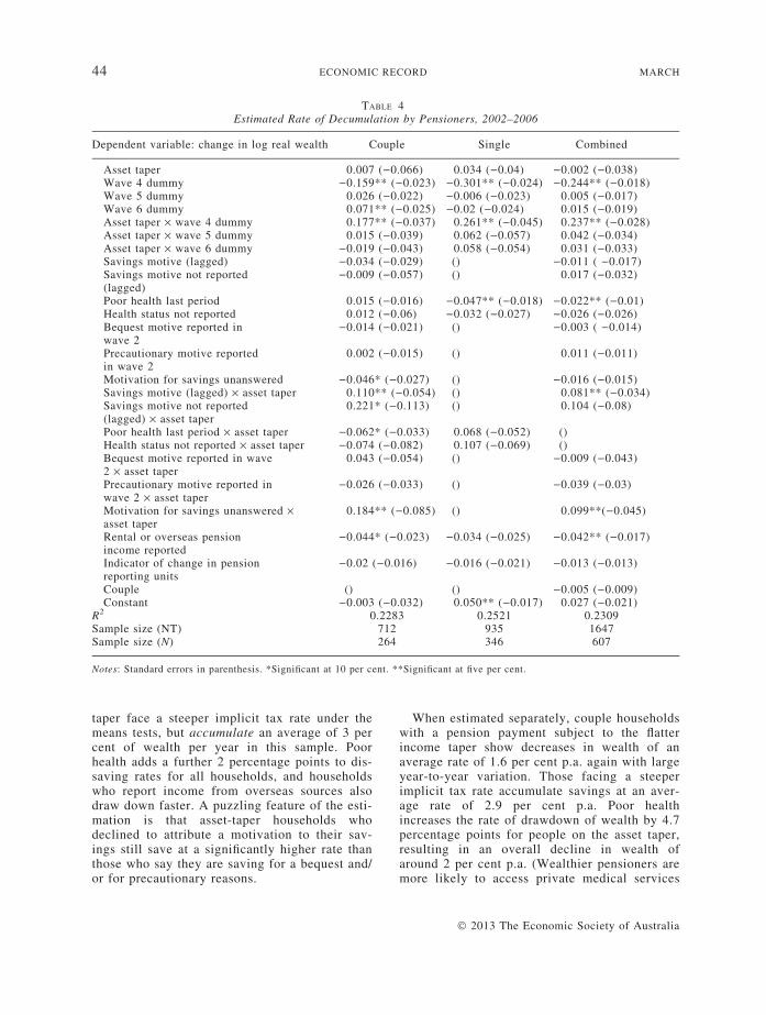
TABLE 4Estimated Rate of Decumulation by Pensioners, 2002–2006
Dependent variable: change in log real wealth Couple Single Combined
Asset taper 0.007 ()0.066) 0.034 ()0.04) )0.002 ()0.038)Wave 4 dummy )0.159** ()0.023) )0.301** ()0.024) )0.244** ()0.018)Wave 5 dummy 0.026 ()0.022) )0.006 ()0.023) 0.005 ()0.017)Wave 6 dummy 0.071** ()0.025) )0.02 ()0.024) 0.015 ()0.019)Asset taper · wave 4 dummy 0.177** ()0.037) 0.261** ()0.045) 0.237** ()0.028)Asset taper · wave 5 dummy 0.015 ()0.039) 0.062 ()0.057) 0.042 ()0.034)Asset taper · wave 6 dummy )0.019 ()0.043) 0.058 ()0.054) 0.031 ()0.033)Savings motive (lagged) )0.034 ()0.029) () )0.011 ( )0.017)Savings motive not reported(lagged)
)0.009 ()0.057) () 0.017 ()0.032)
Poor health last period 0.015 ()0.016) )0.047** ()0.018) )0.022** ()0.01)Health status not reported 0.012 ()0.06) )0.032 ()0.027) )0.026 ()0.026)Bequest motive reported inwave 2
)0.014 ()0.021) () )0.003 ( )0.014)
Precautionary motive reportedin wave 2
0.002 ()0.015) () 0.011 ()0.011)
Motivation for savings unanswered )0.046* ()0.027) () )0.016 ()0.015)Savings motive (lagged) · asset taper 0.110** ()0.054) () 0.081** ()0.034)Savings motive not reported(lagged) · asset taper
0.221* ()0.113) () 0.104 ()0.08)
Poor health last period · asset taper )0.062* ()0.033) 0.068 ()0.052) ()Health status not reported · asset taper )0.074 ()0.082) 0.107 ()0.069) ()Bequest motive reported in wave2 · asset taper
0.043 ()0.054) () )0.009 ()0.043)
Precautionary motive reported inwave 2 · asset taper
)0.026 ()0.033) () )0.039 ()0.03)
Motivation for savings unanswered ·asset taper
0.184** ()0.085) () 0.099**()0.045)
Rental or overseas pensionincome reported
)0.044* ()0.023) )0.034 ()0.025) )0.042** ()0.017)
Indicator of change in pensionreporting units
)0.02 ()0.016) )0.016 ()0.021) )0.013 ()0.013)
Couple () () )0.005 ()0.009)Constant )0.003 ()0.032) 0.050** ()0.017) 0.027 ()0.021)
R2 0.2283 0.2521 0.2309Sample size (NT) 712 935 1647Sample size (N) 264 346 607
Notes: Standard errors in parenthesis. *Significant at 10 per cent. **Significant at five per cent.
44 ECONOMIC RECORD MARCH
taper face a steeper implicit tax rate under themeans tests, but accumulate an average of 3 percent of wealth per year in this sample. Poorhealth adds a further 2 percentage points to dis-saving rates for all households, and householdswho report income from overseas sources alsodraw down faster. A puzzling feature of the esti-mation is that asset-taper households whodeclined to attribute a motivation to their sav-ings still save at a significantly higher rate thanthose who say they are saving for a bequest and/or for precautionary reasons.
When estimated separately, couple householdswith a pension payment subject to the flatterincome taper show decreases in wealth of anaverage rate of 1.6 per cent p.a. again with largeyear-to-year variation. Those facing a steeperimplicit tax rate accumulate savings at an aver-age rate of 2.9 per cent p.a. Poor healthincreases the rate of drawdown of wealth by 4.7percentage points for people on the asset taper,resulting in an overall decline in wealth ofaround 2 per cent p.a. (Wealthier pensioners aremore likely to access private medical services
� 2013 The Economic Society of Australia
2013 MEANS-TESTED PUBLIC PENSIONS 45
and incur additional costs.) Households whichdeclined to comment on health status exhibitedsimilar effects. Singles on the income taperreduced wealth by 6.9 per cent p.a. on averageover 4 years, and on the asset taper, averageincreases in wealth were 3.5 per cent p.a.
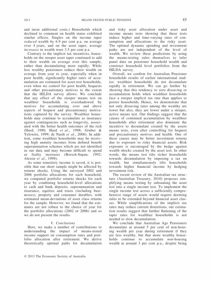
Contrary to the implicit tax incentives, house-holds on the steeper asset taper continued to addto their wealth on average over this sample,rather than decumulating more rapidly. Whileless wealthy pensioners reduce their wealth onaverage from year to year, especially when inpoor health, significantly higher rates of accu-mulation are estimated for asset-test households,even when we control for poor health, bequestsand other precautionary motives to the extentthat the HILDA survey allows. We concludethat any effect of the steeper means test onwealthier households is overshadowed bymotives for accumulating over and aboveaspects of bequest and precautionary motiva-tions captured by the survey. Wealthier house-holds may continue to accumulate as insuranceagainst contingencies such as longevity, associ-ated with the better health outcomes of the rich(Hurd, 1990; Hurd et al., 1998; Gruber &Yelowitz, 1999; de Nardi et al., 2006). In addi-tion, some wealthier households may be receiv-ing high annuity incomes from defined benefitsuperannuation schemes which are not identifiedin our data and may become difficult to spendas frailty increases (Borsch-Supan, 1992;Alessie et al., 1999).
As some transitory income is saved, it is pos-sible that our short sample might be affected byreturns shocks. Using the surveyed 2002 and2006 portfolio allocations for each household,we computed portfolio returns shocks for eachyear by combining household-level allocationsto cash and bank deposits, superannuation andinsurance, equities and trusts (including busi-nesses), property and consumer durables, withestimated mean-deviations of asset class returnsfor the sample. However, we found that the esti-mates are not robust to the choice of year forthe portfolio allocations (2002 or 2006) and sowe do not present the results.
V. ConclusionsHere, we make a number of contributions to
understanding the impact of means-testedincome support on consumption rates and port-folio allocation after retirement. We derivetheoretically optimal paths for decumulation
� 2013 The Economic Society of Australia
and risky asset allocation under asset andincome means tests showing that these testsinduce higher and time-varying rates of con-sumption and allocations to the risky asset.The optimal dynamic spending and investmentpaths are not independent of the level ofwealth. We review these predictions by usingthe means-testing rules themselves to inferpanel data on pensioner household wealth andconstruct household level portfolios from theHILDA survey.
Overall, we confirm for Australian Pensionerhouseholds results of earlier international stud-ies: wealthier households do not decumulaterapidly in retirement. We can go further byshowing that this tendency to zero dissaving oraccumulation holds when wealthier householdsface a steeper implicit tax rate than applies topoorer households. Hence, we demonstrate thatnot only dissaving rates among the wealthy arelower but also, they are lower under a steeper,active means test. Our findings suggest that thecauses of continued accumulation by wealthierhouseholds after retirement also dominate theincentive to decumulate created by the assetsmeans tests, even after controlling for bequestand precautionary motives and health. One ofthese causes may be better investment returnsdue to exposure to risky financial assets. Riskexposure is encouraged by the hedge againstwealth shocks created by the asset test. In otherwords, the means test tilts richer householdstowards decumulation by imposing a tax onwealth, but simultaneously tilts householdstowards higher financial income by hedginginvestment risk.
The recent review of the Australian tax struc-ture (Australian Treasury, 2010) proposes sim-plifying means testing by subsuming the assettest into a single income test. To implement thesingle income test across a sufficiently compre-hensive range of assets would require deemingrules to be extended beyond financial asset clas-ses. While simplifications of the implicit taxrates may reduce current distortions, our estima-tion results suggest that further flattening of thetaper rates for wealthier households is notneeded to slow decumulation.
We conclude that Australian Age Pensionersdecumulate at around 5 per cent of non-hous-ing wealth per year during retirement if theyare less wealthy, but that more wealthy house-holds continue to accumulate non-housingwealth at around 3 per cent p.a., despite being
46 ECONOMIC RECORD MARCH
subject to the incentives of a stricter means-test for pension payments. Portfolio choiceappears to have been one driver of wealthyhousehold accumulations. With some reserva-tions about our small sample, we also find evi-dence that higher risky asset allocations areassociated with higher wealth consistent withour theoretical model.
REFERENCES
Alan, S. and Browning, M. (2006), ‘Estimating Inter-temporal Allocation Parameters using SimulatedExpectation Errors’, Working Paper No. 284, Uni-versity of Oxford, Department of Economics.
Alessie, R., Lusardi, A. and Kapteyn, A. (1999), ‘Sav-ing After Retirement: Evidence from Three Differ-ent Surveys’, Journal of Labour Economics, 6, 277–310.
Attanasio, O., Banks, J., Meghir, C. and Weber, G.(1999), ‘Humps and Bumps in Lifetime Consump-tion’, Journal of Business and Economics Statistics,17, 22–35.
Australian Treasury (2010), Australia’s Future TaxSystem: Final Report. Detailed Analysis Part 2Volume 1, Commonwealth of Australia.
Bateman, H. and Thorp, S. (2008), ‘Choices and Con-straints Over Retirement Income Streams: Compar-ing Rules and Regulations’, Economic Record, 84(s1), s17–31.
Borsch-Supan, A. (1992), ‘Saving and ConsumptionPatterns of the Elderly: The German Case’, Journalof Population Economics, 5, 289–303.
Borsch-Supan, A., Ludwig, A. and Winter, J. (2006),‘Aging, Pension Reform, and Capitalows: A Multi-Country Simulation Model’, Economica, 73, 625–58.
Browning, M. and Crossley, T. (2001), ‘The Life-Cycle Model of Consumption and Saving’, Journalof Economic Perspectives, 15, 3–22.
Butler, M., Peijnenburg, K. and Staubli, S. (2011),‘How Much Do Means-Tested Benefits Reduce theDemand for Annuities?’ Working Paper, SEWHSGUniversity of St.Gallen.
Chand, S. and Jaeger, A. (1996), ‘Aging Populationsand Public Pension Schemes’, Occasional PaperNo. 147, International Monetary Fund.
Cho, S. and Sane, R. (2011), ‘Means Tested Age Pen-sion and Homeownership: Is There a Link?’, Schoolof Economics Discussion Paper 2011/02, Universityof New South Wales.
Coile, C. and Milligan, K. (2009), ‘How HouseholdPortfolios Evolve After Retirement: The Effect ofAging and Health Shocks’, Review of Income andWealth, 55, 226–48.
Commonwealth of Australia (2002), IntergenerationalReport (2002–3). 2002–03 Budget Paper No. 5,Paper prepared by Department of Treasury for theCommonwealth Government Budget, Canberra.
Dynan, K., Skinner, J. and Zeldes, S. (2004), ‘Do theRich Save More?’ Journal of Political Economy, 12,397–444.
Feinstein, J. and Ho, C. (2000), ‘Elderly Asset Man-agement and Health: An Empirical Analysis’,Working Paper No. 7814, National Bureau of Eco-nomic Research.
Gourinchas, C. and Parker, J. (2002), ‘ConsumptionOver the Life Cycle’, Econometrica, 70, 47–89.
Gruber, J. and Wise, D. (2005). Social Security Pro-grams and Retirement Around the World: FiscalImplications of Reform. University of ChicagoPress, London UK.
Gruber, J. and Yelowitz, A. (1999), ‘Public HealthInsurance and Private Savings’, Journal of PoliticalEconomy, 107, 1249–74.
Harmer, J. (2008), ‘Pension Review’, Backgroundpaper, Department of Families, Housing, Commu-nity Services and Indigenous Affairs, Canberra.
Hubbard, R.G., Skinner, J. and Zeldes, S.P. (1995),‘Precautionary Saving and Social Insurance’, Jour-nal of Political Economy, 103, 360–99.
Hurd, M. (1990), ‘Research on the Elderly: EconomicStatus, Retirement, and Consumption and Saving’,Journal of Economic Literature, 28, 565–637.
Hurd, M., McFadden, D. and Merrill, A. (1998), ‘Pre-dictors of Mortality among the Elderly’, WorkingPaper No. 7440, National Bureau of EconomicResearch.
Hurst, E. and Ziliak, J. (2006), ‘Do Welfare AssetLimits Affect Household Saving? Evidence fromWelfare Reform’, Journal of Human Resources, 41,46–71.
Ingersoll, J. (1987), The Theory of Financial DecisionMaking. Rowman and Littlefield, Savage, MA.
Kelly, S. (2009), Reform of the Australian RetirementIncome System. Research Report, NATSEM, Uni-versity of Canberra, Canberra.
de Nardi, M., French, E. and Jones, J. (2006), ‘Dif-ferential Mortality, Uncertain Medical Expenses,and the Saving of Elderly Singles’, Working PaperNo. 12554, National Bureau of EconomicResearch.
Neumark, D. and Powers, E. (1998), ‘The Effect ofMeans Tested Income Support for the Elderly onPre-Retirement Saving: Evidence from the SSI Pro-gram in the US’, Journal of Public Economics, 68,181–206.
Neumark, D. and Powers, E. (2000), ‘Welfare for theElderly: The Effects of SSI on Pre-RetirementLabour Supply’, Journal of Public Economics, 78,51–80.
Novy-Marx, R. and Rauh, J. (2008), ‘The Intergenera-tional Transfer of Public Pension Promises’, Work-ing Paper No. 14343, National Bureau of EconomicResearch.
Petrichev, K. and Thorp, S. (2008), ‘The PrivateValue of Public Pensions’, Insurance: Mathematicsand Economics, 42, 1138–45.
� 2013 The Economic Society of Australia
2013 MEANS-TESTED PUBLIC PENSIONS 47
Sefton, J., van de Ven, J. and Weale, M. (2008),‘Means Testing Retirement Benefits: FosteringEquity or Discouraging Savings?’, Economic Jour-nal, 188, 556–90.
Sinai, T. and Souleles, N. (2007), ‘Net Worth andHousing Equity in Retirement’, Working Paperw13693, National Bureau of Economic Research.
Thorp, S., Kingston, G. and Bateman, H. (2007),‘Financial Engineering for Australian Annuitants’,
� 2013 The Economic Society of Australia
in Bateman, H. (ed.), Retirement Provision inScary Markets. Edward Elgar, Cheltenham; 123–44.
Wachter, J. and Yogo, M. (2010), ‘Why Do House-hold Portfolio Shares Rise in Wealth?’ Review ofFinancial Studies, 23, 3929–65.
Ziliak, J. (2003), ‘Income Transfers and Assets of thePoor’, Review of Economics and Statistics, 85, 63–76.
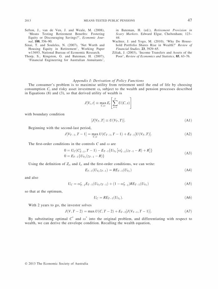
Appendix I: Derivation of Policy FunctionsThe consumer’s problem is to maximise utility from retirement until the end of life by choosing
consumption Ct and risky asset investment xt subject to the wealth and pension processes describedin Equations (8) and (3), so that derived utility of wealth is
J½Vt; t� � maxC;x
Et
XT
s¼t
UðC; sÞ" #
with boundary condition
½J½VT ; T� � UðVT ; TÞ�: ðA1Þ
Beginning with the second-last period,
J½VT�1; T � 1� ¼ maxC;w
UðCT�1; T � 1Þ þ ET�1½UðVT ; TÞ�: ðA2Þ
The first-order conditions in the controls C and x are
0 ¼ UCðC�T�1; T � 1Þ � ET�1fUVT x�T�1ðzT�1 � RÞ þ R� �
g0 ¼ ET�1fUVT ðzT�1 � RÞg
ðA3Þ
Using the definition of Zt, and It, and the first-order conditions, we can write:
ET�1ðUVT zT�1Þ ¼ RET�1ðUVT Þ ðA4Þ
and also
UC ¼ x�T�1ET�1ðUVT zT�1Þ þ ð1� x�T�1ÞRET�1ðUVT Þ ðA5Þ
so that at the optimum,
UC ¼ RET�1ðUVT Þ: ðA6Þ
With 2 years to go, the investor solves
JðV ; T � 2Þ ¼ max UðC; T � 2Þ þ ET�2½JðVT�1; T � 1Þ�: ðA7Þ
By substituting optimal C* and x* into the original problem, and differentiating with respect towealth, we can derive the envelope condition. Recalling the wealth equation,
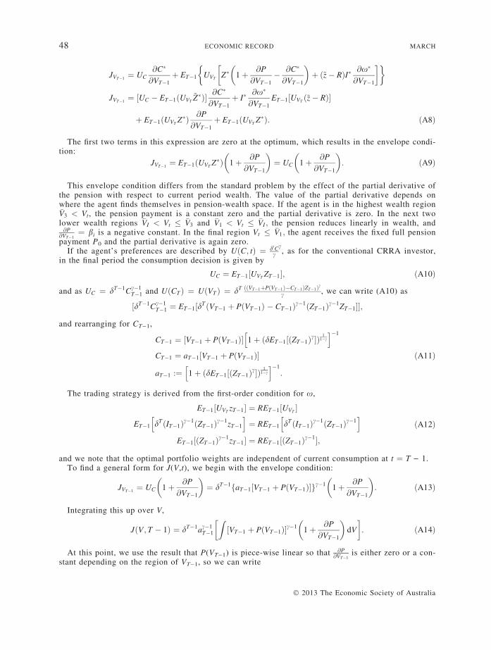
48 ECONOMIC RECORD MARCH
JVT�1 ¼ UC@C�
@VT�1þ ET�1 UVT Z� 1þ @P
@VT�1� @C�
@VT�1
� �þ ð~z� RÞI� @x�
@VT�1
� � �
JVT�1 ¼ ½UC � ET�1ðUVT~Z�Þ� @C�
@VT�1þ I�
@x�
@VT�1ET�1½UVT ð~z� RÞ�
þ ET�1ðUVT Z�Þ @P
@VT�1þ ET�1ðUVT Z�Þ: ðA8Þ
The first two terms in this expression are zero at the optimum, which results in the envelope condi-tion:
JVT�1 ¼ ET�1ðUVT Z�Þ 1þ @P
@VT�1
� �¼ UC 1þ @P
@VT�1
� �: ðA9Þ
This envelope condition differs from the standard problem by the effect of the partial derivative ofthe pension with respect to current period wealth. The value of the partial derivative depends onwhere the agent finds themselves in pension-wealth space. If the agent is in the highest wealth region�V3 < Vt, the pension payment is a constant zero and the partial derivative is zero. In the next twolower wealth regions �VI < Vt � �V3 and �V1 < Vt � �VI ; the pension reduces linearly in wealth, and@P
@VT�1¼ bi is a negative constant. In the final region Vt � �V1; the agent receives the fixed full pension
payment P0 and the partial derivative is again zero.If the agent’s preferences are described by UðC; tÞ ¼ dtC
c
c, as for the conventional CRRA investor,
in the final period the consumption decision is given by
UC ¼ ET�1½UVT ZT�1�; ðA10Þ
and as UC ¼ dT�1Cc�1T�1 and UðCTÞ ¼ UðVTÞ ¼ dT ððVT�1þPðVT�1Þ�CT�1ÞZT�1Þc
c , we can write (A10) as
½dT�1Cc�1T�1 ¼ ET�1½dTðVT�1 þ PðVT�1Þ � CT�1Þc�1ðZT�1Þc�1ZT�1��;
and rearranging for CT)1,
CT�1 ¼ ½VT�1 þ PðVT�1Þ� 1þ ðdET�1½ðZT�1Þc�Þ1
1�c
h i�1
CT�1 ¼ aT�1½VT�1 þ PðVT�1Þ�
aT�1 :¼ 1þ ðdET�1½ðZT�1Þc�Þ1
1�c
h i�1:
ðA11Þ
The trading strategy is derived from the first-order condition for x,
ET�1½UVT zT�1� ¼ RET�1½UVT �
ET�1 dTðIT�1Þc�1 ZT�1ð Þc�1zT�1
h i¼ RET�1 dTðIT�1Þc�1 ZT�1ð Þc�1
h iET�1½ ZT�1ð Þc�1zT�1� ¼ RET�1½ ZT�1ð Þc�1�;
ðA12Þ
and we note that the optimal portfolio weights are independent of current consumption at t ¼ T ) 1.To find a general form for J(V,t), we begin with the envelope condition:
JVT�1 ¼ UC 1þ @P
@VT�1
� �¼ dT�1faT�1½VT�1 þ PðVT�1Þ�gc�1 1þ @P
@VT�1
� �: ðA13Þ
Integrating this up over V,
JðV ; T � 1Þ ¼ dT�1ac�1T�1
Z½VT�1 þ PðVT�1Þ�c�1 1þ @P
@VT�1
� �dV
� : ðA14Þ
At this point, we use the result that P(VT)1) is piece-wise linear so that @P@VT�1
is either zero or a con-stant depending on the region of VT)1, so we can write
� 2013 The Economic Society of Australia
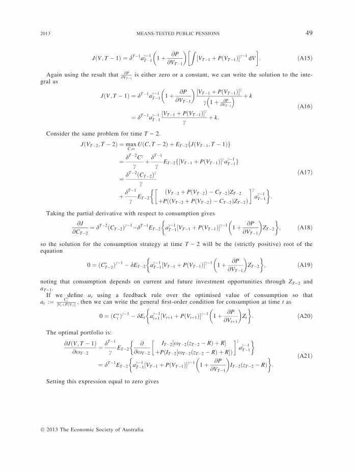
2013 MEANS-TESTED PUBLIC PENSIONS 49
JðV ; T � 1Þ ¼ dT�1ac�1T�1 1þ @P
@VT�1
� � ZVT�1 þ P VT�1ð Þ½ �c�1 dV
� : ðA15Þ
Again using the result that @P@VT�1
is either zero or a constant, we can write the solution to the inte-gral as
JðV ; T � 1Þ ¼ dT�1ac�1T�1 1þ @P
@VT�1
� �VT�1 þ P VT�1ð Þ½ �c
c 1þ @P@VT�1
� þ k
¼ dT�1ac�1T�1½VT�1 þ PðVT�1Þ�c
cþ k:
ðA16Þ
Consider the same problem for time T ) 2.
JðVT�2; T � 2Þ ¼ maxC;x
UðC; T � 2Þ þ ET�2fJðVT�1; T � 1Þg
¼ dT�2Cc
cþ dT�1
cET�2f½VT�1 þ PðVT�1Þ�cac�1
T�1g
¼ dT�2ðCT�2Þc
c
þ dT�1
cET�2
ðVT�2 þ PðVT�2Þ � CT�2ÞZT�2
þPððVT�2 þ PðVT�2Þ � CT�2ÞZT�2Þ
� c
ac�1T�1
� �:
ðA17Þ
Taking the partial derivative with respect to consumption gives
@J
@CT�2¼ dT�2 CT�2ð Þc�1�dT�1ET�2 ac�1
T�1 VT�1 þ P VT�1ð Þ½ �c�1 1þ @P
@VT�1
� �ZT�2
� �; ðA18Þ
so the solution for the consumption strategy at time T ) 2 will be the (strictly positive) root of theequation
0 ¼ ðC�T�2Þc�1 � dET�2 ac�1
T�1 VT�1 þ P VT�1ð Þ½ �c�1 1þ @P
@VT�1
� �ZT�2
� �; ðA19Þ
noting that consumption depends on current and future investment opportunities through ZT)2 andaT)1.
If we define at using a feedback rule over the optimised value of consumption so thatat :¼ C�t
½VtþPðVtÞ� ; then we can write the general first-order condition for consumption at time t as
0 ¼ ðC�t Þc�1 � dEt ac�1
tþ1 ½Vtþ1 þ PðVtþ1Þ�c�1 1þ @P
@Vtþ1
� �Zt
� �: ðA20Þ
The optimal portfolio is:
@JðV ; T � 1Þ@xT�2
¼ dT�1
cET�2
@
@xT�2
IT�2 xT�2 zT�2 � Rð Þ þ R½ �þP IT�2 xT�2 zT�2 � Rð Þ þ R½ �ð Þ
� c
ac�1T�1
� �
¼ dT�1ET�2 ac�1T�1 VT�1 þ P VT�1ð Þ½ �c�1 1þ @P
@VT�1
� �IT�2 zT�2 � Rð Þ
� �:
ðA21Þ
Setting this expression equal to zero gives
� 2013 The Economic Society of Australia
50 ECONOMIC RECORD MARCH
ET�2 ac�1T�1 VT�1 þ P VT�1ð Þ½ �c�1 1þ @P
@VT�1
� �zT�2 � Rð Þ
� �¼ 0 ðA22Þ
E ac�1 I� Z� þ P I� Z�� � �c�1
1þ @P� �
z
� �
T�2 T�1 T�2 T�2 T�2 T�2 @I�T�2Z�T�2T�2
¼ RET�2 ac�1T�1 I�T�2Z�T�2 þ P I�T�2Z�T�2
� � �c�11þ @P
@I�T�2Z�T�2
� �� �:
ðA23Þ
The optimal trading strategy x(/) therefore depends on future investment opportunities via aT)1
and the current consumption strategy via I�T�2:
Appendix II: Construction of Wealth Measures in Figures 5a and 6bFigure 5a: we stack all reporting households (5253 households) and the subset of households
reporting receipt of the Age Pension (795 households whose heads answer ‘yes’ to PQ F12a: ‘Do youcurrently receive the Age Pension from the Australian Federal Government?’ i.e. FBNCAP ¼ 1)Household Total Assets ($) FHWASSET DV, select the 20 per cent, 40 per cent, 60 per cent, and 80per cent quantiles and graph the mean of each.
Figure 5b: we stack all reporting households (5253 households), households with head over65 years (1116) and households reporting receipt of the Age Pension (795) by FHWFIN, select the 20per cent, 40 per cent, 60 per cent, and 80 per cent quantiles and graph the mean of each. FHWFIN isDV: Household Financial Assets ($), the sum of household equity investments (FHWEQINV), cashinvestments (FHWCAIN), trusts (FHWTRUST), own bank accounts (FHWOBANK), joint bankaccounts (FHWJBANK), children’s bank accounts (FHWCBANK), redeemable insurance policies(FHWINSUR), retirees superannuation (FHWSUPRT), and non-retirees superannuation(FHWSUPWK).
Figure 6a: we compute the average percentage by quintile of Age Pension households’ total assetsFHWASSET allocated to each of the following categories: Public equity: FHWEQINV (Total shares,managed funds, and property trusts for the household) + FHWTRUST (Total household wealth intrust funds (including children’s trust funds); Safe assets: FHWTBANK (Sum of individual level bankaccounts (FHWOBANK), individual level joint bank accounts (FHWJBANK) and household levelchildren’s bank accounts (FHWCBANK) + FHWCAIN (Government bonds, corporate bonds, deben-tures, certificates of deposit, and mortgage backed securities owned by the household); Insurance:FHWINSUR redeemable insurance policies; Superannuation: FHWSUPER retirees superannuation(FHWSUPRT) + non-retirees superannuation (FHWSUPWK); Vehicles: FHWVECH The sum of thevalue of transport vehicles (cars, vans, motorbikes, tucks, utilities), recreational vehicles (boats, cara-vans, campervans, jet skis, trail bikes) and tractors, planes, helicopters and other vehicles at thehousehold level; Property: FHWTPVAL Sum of home value (FHWHMVAL) and other property value(FHWOPVAL) at the household level. Does not include home contents; Business: FHWBUSVA Busi-ness/farm assets owed by the household. Excludes assets owed by individuals outside the household;Collectibles: FHWCOLL Total of substantial assets such as antiques, works of art, and collectiblesfor the household.
Figure 6b: we compute the average percentage by quintile of Age Pension households’ total assetsFHWASSET less the value of the home, FHWHMVAL, allocated to each of the categories describedfor Figure 6a but where property is other property, FHWOPVAL only.
Appendix III: Definitions of Panel Survey Indicator VariablesSavings motive lagged ¼ 1 if at least one member of the household answers the question ‘Which
of the following statements comes closest to describing your (and your family’s) savings habits?’ as
• Save whatever is leftover – no regular plan• Spend regular income save other income• Save regularly by putting money aside each month
� 2013 The Economic Society of Australia
2013 MEANS-TESTED PUBLIC PENSIONS 51
in the previous wave. In wave 5, this question was not asked and as such in wave 6 this variableproxies using the answer for wave 6. Savings motive not reported lagged ¼ 1 if no one in thehousehold provides an answer to the question ‘Which of the following statements comes closest todescribing your (and your family’s) savings habits?’. In wave 5, this question was not asked and assuch in wave 6 this variable proxies using the answer for wave 6.
Poor health last period ¼ 1 if at least one household member reports general health as ‘fair’ or‘poor’, and zero if ‘good’, ‘very good’, ‘excellent’ or declined to comment in the previous wave.Health status not reported ¼ 1 if all households members declined to comment on health status inthe previous wave.
Bequest motive reported in wave 2 ¼ 1 if the household answers yes to at least one of the follow-ing question in the 2002 wave: ‘Which of the following comes closest to describing your (and yourfamily’s) current reason for saving? (i) Education for children and grandchildren; and/or (ii) To helpchildren or other relatives’.
Precautionary motive reported in wave 2 ¼ 1 if the household answers yes to at least one of thefollowing questions in the 2002 wave: ‘Which of the following comes closest to describing your (andyour family’s) current reason for saving?’ (i) For emergencies/in case of unemployment or illness;and/or (ii) Medical/dental expenses.
Motivation for savings not reported ¼ 1 if all members of the household declined to answer thequestion ‘Which of the following comes closest to describing your (and your family’s) current reasonfor saving?’.
Rental or overseas pension income reported ¼ 1 if the household reports receiving income fromrental properties or overseas pensions and 0 if not.
Indicator of change in pension reporting units ¼ 1 if at least one member of the household haschanged from reporting their pension in average weekly terms to annual terms or vice versa.
� 2013 The Economic Society of Australia