Measurement of the CP asymmetry in the decay B0→K−π+

with the LHCb detector

Miriam Heß, Christian Voß, Roland Waldi

April 12, 2013

Institut fur PhysikUniversitat Rostock

18051 Rostock

Advisor: Miriam Heß (miriam.hess@cern.ch)

1

Abstract

The aim of this lab experiment is to measure the direct CP asymmetry in the decayB→Kπ, defined in terms of the decay rates as

ACP (B→Kπ) =N(B0→K−π+

)−N (B0→K+π−)

N(B0→K−π+

)+N (B0→K+π−)

.

In order to measure the number of B0→K−π+ events (and its charge conjugatedmode) the decay has to be reconstructed from data collected with the LHCb experiment.The number of events can be determined in the invariant B mass distribution.

2

Contents

1 Conventions 4

2 Preparation 4

3 Introduction 43.1 Two-body decay kinematics . . . . . . . . . . . . . . . . . . . . . . . . . . . . 43.2 The CKM matrix . . . . . . . . . . . . . . . . . . . . . . . . . . . . . . . . . . 53.3 CP violation . . . . . . . . . . . . . . . . . . . . . . . . . . . . . . . . . . . . 63.4 Theory of B→Kπ decays . . . . . . . . . . . . . . . . . . . . . . . . . . . . . 7

4 The LHCb experiment 74.1 Kaon and pion identification . . . . . . . . . . . . . . . . . . . . . . . . . . . . 8

5 Tasks 9

6 Kinematic reconstruction of a decay 96.1 Reconstruction with DaVinci . . . . . . . . . . . . . . . . . . . . . . . . . . . 106.2 Event selection . . . . . . . . . . . . . . . . . . . . . . . . . . . . . . . . . . . 126.3 Analysing histograms . . . . . . . . . . . . . . . . . . . . . . . . . . . . . . . . 14

6.3.1 Peaking background . . . . . . . . . . . . . . . . . . . . . . . . . . . . 156.3.2 Usage of simulated events . . . . . . . . . . . . . . . . . . . . . . . . . 156.3.3 Fitting the invariant mass distribution . . . . . . . . . . . . . . . . . . 166.3.4 Calculate the CP asymmetry . . . . . . . . . . . . . . . . . . . . . . . 17

3

1 Conventions

In particle physics, we use natural units c and ~ together with electron volt ( eV) and itsmultiples (e.g. keV, MeV, GeV, . . . ). In everyday life, formulae and calculations simplifyconsiderable if we omit the c and ~, setting c = ~ = 1. Then, eV is the unit for energies,momenta and masses and we can write E2 = m2 + p2 instead of E2 = m2c4 + p2c2.

2 Preparation

Read this manual carefully and prepare the following questions and themes.

• What is direct CP violation and when can it be measured?

• What is the expected CP asymmetry in the decay B0→K−π+ you are going to measurein this lab experiment?

• Which kind of detector is used at LHCb in order to distingush between kaon and pions?And how does it work?

• Remind yourself of the quark sector of the weak interaction, especially the CKM matrix.

• Inform yourself of the discrete transformations of parity, charge and the product ofcharge and parity.

Knowledge of C++ programming language is appreciated, but not mandatory, as is knowl-edge of statistical data analysis methods. An introduction into the necessary functions isgiven in the corresponding section 6.

3 Introduction

The LHCb detector is located at the Large Hadron Collider (LHC) located at the site of theCERN laboratory near Geneva at the Swiss-French border. CERN is named after its foundingbody Conseil Europeen pour la Recherche Nucleaire. The dataset under investigation in thislab exercise was taken in 2011 at a centre of mass energy of 7 TeV. Its main purpose is tostudy the decays of charm and beauty hadrons, which are produced in the strong interactionsof the colliding protons. Beauty quarks produced at the LHC are generally produced with lowtransverse momenta. This required a dedicated design for the detector. It almost resemblesa detector for a fixed-target experiment and is able to detect charged particles and photonsat small angles to the proton beams.

In the following sections a basic introduction into relativistic kinematics, the weak inter-action, and direct CP violation in B→Kπ decays is given. B mesons are bound states of theheavy beauty quark and a light quark.

3.1 Two-body decay kinematics

The two-body decay B0→K−π+ is determined by conservation of energy and momentum:

EB = EK + Eπ (1)pB = pK + pπ . (2)

4

A Lorentz-invariant quantity is the invariant mass given by

m2B = E2

B − p2B . (3)

in any reference frame.In the rest frame of the B0 meson the relations reduce to

mB = E∗K + E∗π (4)0 = p∗K + p∗π . (5)

With the relativistic relation E2 = m2 + p2, the absolute values of momenta can be writtenas

p∗K = p∗π = p∗ =1

2mB

√(m2B − (mK +mπ)2

) (m2B − (mK −mπ)2

)The Lorentz-invariant phase space volume enters the decay probability as a statistical

contribution. For any two-body final state from a decay it is proportional to this momentump∗ in the mother particle’s rest frame.

Momentum vectors ara given in a Cartesian coordinate system where the z axis points inthe direction of the colliding beams. The transverse momentum is defined as

pT =√p2x + p2

y . (6)

The advantage of this variable is that it is Lorentz-invariant under boosts along the z axis,and almost invariant when we transform between the B system and the detector rest system,since the B mesons go at small angles to the z axis.

3.2 The CKM matrix

In charged current weak decays (i.e., couplings to the W± bosons), quarks are allowed todecay into any other quark differing by one elementary charge. While the quark state |b〉 isan eigenstate of the strong interaction (distinguished from other quark states by its mass),it is not an eigenstate of the weak interaction due to the quark-mixing. The weak eigenstate|b′〉 is defined as

|b′〉 = Vtd|d〉+ Vts|s〉+ Vtb|b〉 , (7)

with components of all possible quark flavours. The factor Vtd, for instance, determines theamplitude 〈d | b′〉 = Vtd to find a |d〉 quark in the |b′〉 state, since the top quark t is theweak interaction partner of the b′ quark. These elements form a unitary 3 × 3 matrix, theCabibbo-Kobayashi-Maskawa (CKM) matrix

V =

Vud Vus VubVcd Vcs VcbVtd Vts Vtb

. (8)

Due to its unitarity and the non-observability of several phases, its number of free parametersis reduced to three mixing angles and one complex phase [1; 2; 3]. The unitarity of the

5

CKM matrix leads to twelve equations, where six relations describe unitarity triangles in thecomplex plane. One of this relations is

V ∗udVtd + V ∗usVts + V ∗ubVtb = 0 . (9)

Figure 1 visualises this relation in the complex plane. In contrast to phases attached toindividual CKM matrix elements, which can be changed by convention with the phases ofthe quark fields, the phases represented by the angles of unitarity triangles are invariantunder such phase transformations. Therefore, these angles are observables and are used todescribe interference effects induced by the CKM matrix, in particular CP violation.

Im

Re......................................................................................................................................................................................................................................................................................................................................................................................................................................................................

............................................

............................................

............................................

............................................

............................................

............................................

...........................................................

..............................................................................................................................................................................................................................................................................

β′γ′

V ∗usVts

V ∗udVtdV ∗ubVtb

α

Figure 1: Unitary triangle (orthogonality of the first and third row of the CKM matrix) in the complexplane

A possible parametrisation of the CKM matrix, which uses a choice of phases leaving Vudand Vcb real, is given by

V =

|Vud| |Vus| |Vub|e−ıγ−|Vcd|eıφ4 |Vcs|e−ıφ6 |Vcb||Vtd|e−ıβ −|Vts|eıφ2 |Vtb|

. (10)

The phases φ2, φ4 and φ6 are relatively small and can be neglected. Therefore we have

γ′ = γ − φ2 ≈ γ ≈ γ

where γ = γ − φ4 is an angle of another unitarity triangle.

3.3 CP violation

The complex phase of the CKM matrix is the only source for CP violation within the Stan-dard Model. There are three possible sources for CP violation, direct CP violation, themixing induced CP violation, in which decays of mixed (B0→B0) and unmixed (B0→B0)mesons interfere, and CP violation in the mixing process itself. In general CP violation is aninterference effect. Direct CP violation is observable in a decay and its CP conjugate decaywhen at least two amplitudes interfere with different CKM phases and different strong phasesare necessary.

6

In order to determine the CP violating asymmtery the following quantity is used,

ACP (B→Kπ) =N(B0→K−π+

)−N (B0→K+π−)

N(B0→K−π+

)+N (B0→K+π−)

, (11)

where B0→K−π+ is the decay under study, B0→K+π− its CP conjugate decay. N is thenumber of decays in a sample of an equal number of B0 and B0 mesons.

3.4 Theory of B→Kπ decays

b

d

s

u

u

d

B0 K−

π+

b

b

d

dB0

s

uK−

d

uπ+

W−

t

W−

(a) (b)

Figure 2: Feyman diagrams for the decay B→Kπ. (a) penguin diagram (b) tree diagram

The B0 decays, studied in this exercise, follow the penguin diagram (Fig. 2a) and treediagram (Fig. 2b). The combination of us makes up a K−, the ud a π+, and for the B0 theud a π− and the su a K+ meson. The tree diagram is proportional to the matrix elementsVubV

∗us and the penguin amplitude is proportional to VtbV ∗ts. These two different mechanisms,

carrying different weak and strong phases, lead to a measurable CP violating asymmetry.The amplitudes for the decay under study is defined as follows

A(B0→K+π−) = |A1|eıδ1+ıγ + |A2|eıδ2+ıφ2 (12)

A(B0→K−π+) = |A1|eıδ1−ıγ + |A2|eıδ2−ıφ2 , (13)

where the first term refers to the contribution of the tree diagram and the second to thecontribution of the penguin diagram. The strong phases are denoted by δi. Strong phases donot change under a CP transformation, hence strong interaction conserves the CP sysmmetry.In contrast, CKM phases are CP -odd, i.e., they change sign under a CP transformation. TheCP violating asymmetry is

ACP ≡ A2 − A2

A2 + A2=

2|A1||A2| sin(δ) sin(γ − φ2)|A1|2 + |A2|2 + 2|A1||A2| cos(δ) cos(γ − φ2)

, (14)

where δ = δ1 − δ2. Obviously, an asymmetry requires both δ1 6= δ2 and a difference in CKMphases for the two interfering amplitudes.

4 The LHCb experiment

The LHCb detector, fig. 3, consists of a silicon strip detector (VELO) located around theinteraction point, used to measure charged particles and decay vertices with high precision.

7

The Tracker Turicensis (TT, built in Zurich, also Trigger Tracker or Target Tracker) consistingof microstrip silicon sensors provides additional information on charged tracks in front of themagnet. Behind the magnet there are three tracking stations, T1,T2, and T3. The innerpart, the Inner Tracker (IT), is similar to the TT, whereas the outer parts, the Outer Tracker(OT), consists of drift chambers. The deflection of charged particles in the magnetic field isused to determine their momenta. The measurements in front of the magnet and behind themagnet are used for that purpose.

Behind the tracking stations, there are two calorimeters used to distinguish electrons andhadrons like pions und kaons. The final section consists of the muon chambers. For additionalinformation see [5].

Figure 3: The LHCb detector

4.1 Kaon and pion identification

To distinguish kaons from pions, the characteristic Cherenkov angle is used. There aretwo Cherenkov detectors, one located upstream (in front of), the other located downstream(behind) the magnet.

The Cherenkov detectors help to discriminate kaons from pions up to momenta of100 GeV. Charged particles passing through matter faster than the speed of light in themedium emit Cherenkov light along their path. The aperture angle with respect to theparticle’s track is called the Cherenkov angle θC . It is defined as

cos θC = 1/nβ , (15)

where n is the refractive index of the material and β = v/c is the velocity of the particle.Therefore, the Cherenkov angle allows to measure the particle’s velocity. In combinationwith the momentum measurement, provided by the tracking system, the mass of a particle

8

can be determined. The mass is unique for each type of particle and thus allows to separatethem.

Fig. 4 shows the dependency of the Cherenkov angle on the momentum for severalcharged particles measured with the Cherenkov detectors.

Figure 4: Cherenkov angle of certain particles in the three Cherenkov media

5 Tasks

1. Reconstruct the decays B0→K−π+ and B0→K+π−

2. Improve the signal to background ratio using dedicated selection criteria

3. Use simulated events for B → Kπ, B → K−K+, B → π−π+, and Bs → K−π+ todetermine their shape

4. Fit the invariant B mass using these shapes and extract the CP -asymmetry

6 Kinematic reconstruction of a decay

Event reconstruction provides a list of charged particles, with their four-momenta, estimatedmomentum uncertainties and a particle type hypothesis. The reconstruction is performedby a framework called Brunel. Next step and main purpose of this exercise is to use thesecharged particles to reconstruct their instable mothers, whose lifetime is too short to bereconstructed by the detector. This is done with DaVinci. Your first task is to provide aprogram module for DaVinci.

For measuring the frequency for B0 mesons decaying into K−π+ and B0→K+π−, onehas to count these decays. Therefore, for every combination of K and π mesons, the invariantmass of the tracks has to be calculated, i.e. the square root of the four-momentum squared.

9

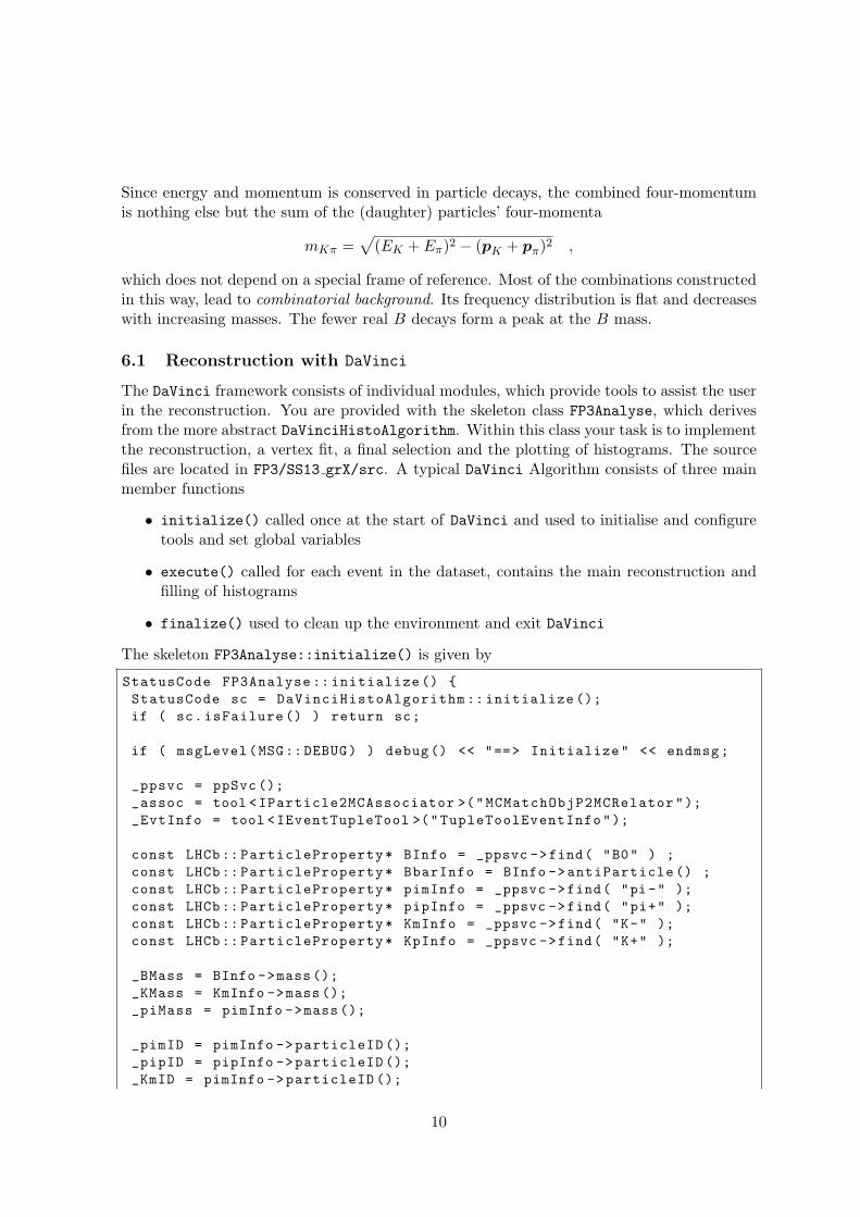
Since energy and momentum is conserved in particle decays, the combined four-momentumis nothing else but the sum of the (daughter) particles’ four-momenta

mKπ =√

(EK + Eπ)2 − (pK + pπ)2 ,

which does not depend on a special frame of reference. Most of the combinations constructedin this way, lead to combinatorial background. Its frequency distribution is flat and decreaseswith increasing masses. The fewer real B decays form a peak at the B mass.

6.1 Reconstruction with DaVinci

The DaVinci framework consists of individual modules, which provide tools to assist the userin the reconstruction. You are provided with the skeleton class FP3Analyse, which derivesfrom the more abstract DaVinciHistoAlgorithm. Within this class your task is to implementthe reconstruction, a vertex fit, a final selection and the plotting of histograms. The sourcefiles are located in FP3/SS13 grX/src. A typical DaVinci Algorithm consists of three mainmember functions

• initialize() called once at the start of DaVinci and used to initialise and configuretools and set global variables

• execute() called for each event in the dataset, contains the main reconstruction andfilling of histograms

• finalize() used to clean up the environment and exit DaVinci

The skeleton FP3Analyse::initialize() is given by

StatusCode FP3Analyse :: initialize () {StatusCode sc = DaVinciHistoAlgorithm :: initialize ();if ( sc.isFailure () ) return sc;

if ( msgLevel(MSG:: DEBUG) ) debug() << "==> Initialize" << endmsg;

_ppsvc = ppSvc ();_assoc = tool <IParticle2MCAssociator >("MCMatchObjP2MCRelator");_EvtInfo = tool <IEventTupleTool >("TupleToolEventInfo");

const LHCb:: ParticleProperty* BInfo = _ppsvc ->find( "B0" ) ;const LHCb:: ParticleProperty* BbarInfo = BInfo ->antiParticle () ;const LHCb:: ParticleProperty* pimInfo = _ppsvc ->find( "pi-" );const LHCb:: ParticleProperty* pipInfo = _ppsvc ->find( "pi+" );const LHCb:: ParticleProperty* KmInfo = _ppsvc ->find( "K-" );const LHCb:: ParticleProperty* KpInfo = _ppsvc ->find( "K+" );

_BMass = BInfo ->mass ();_KMass = KmInfo ->mass ();_piMass = pimInfo ->mass ();

_pimID = pimInfo ->particleID ();_pipID = pipInfo ->particleID ();_KmID = pimInfo ->particleID ();

10

_KpID = pipInfo ->particleID ();

return StatusCode :: SUCCESS;}

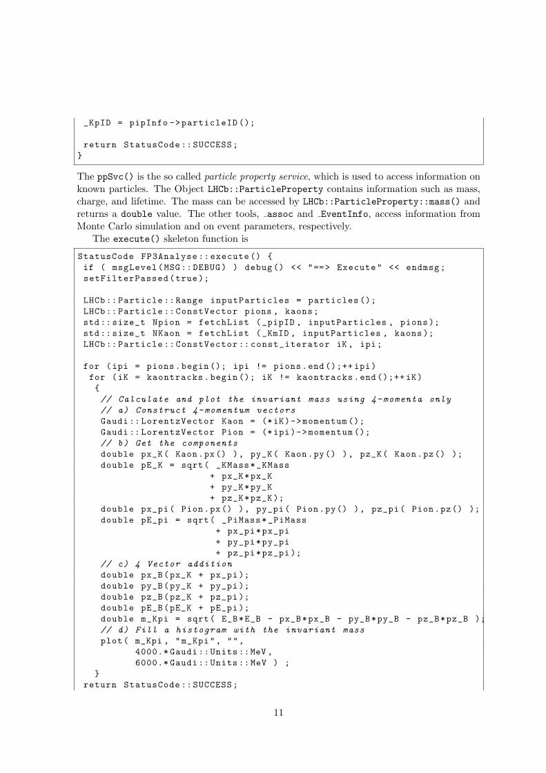
The ppSvc() is the so called particle property service, which is used to access information onknown particles. The Object LHCb::ParticleProperty contains information such as mass,charge, and lifetime. The mass can be accessed by LHCb::ParticleProperty::mass() andreturns a double value. The other tools, assoc and EventInfo, access information fromMonte Carlo simulation and on event parameters, respectively.

The execute() skeleton function is

StatusCode FP3Analyse :: execute () {if ( msgLevel(MSG:: DEBUG) ) debug() << "==> Execute" << endmsg;setFilterPassed(true);

LHCb:: Particle :: Range inputParticles = particles ();LHCb:: Particle :: ConstVector pions , kaons;std:: size_t Npion = fetchList (_pipID , inputParticles , pions);std:: size_t NKaon = fetchList (_KmID , inputParticles , kaons);LHCb:: Particle :: ConstVector :: const_iterator iK , ipi;

for (ipi = pions.begin (); ipi != pions.end ();++ ipi)for (iK = kaontracks.begin (); iK != kaontracks.end ();++iK){// Calculate and plot the invariant mass using 4-momenta only

// a) Construct 4-momentum vectors

Gaudi :: LorentzVector Kaon = (*iK)->momentum ();Gaudi :: LorentzVector Pion = (*ipi)->momentum ();// b) Get the components

double px_K( Kaon.px() ), py_K( Kaon.py() ), pz_K( Kaon.pz() );double pE_K = sqrt( _KMass*_KMass

+ px_K*px_K+ py_K*py_K+ pz_K*pz_K);

double px_pi( Pion.px() ), py_pi( Pion.py() ), pz_pi( Pion.pz() );double pE_pi = sqrt( _PiMass*_PiMass

+ px_pi*px_pi+ py_pi*py_pi+ pz_pi*pz_pi );

// c) 4 Vector addition

double px_B(px_K + px_pi);double py_B(py_K + py_pi);double pz_B(pz_K + pz_pi);double pE_B(pE_K + pE_pi);double m_Kpi = sqrt( E_B*E_B - px_B*px_B - py_B*py_B - pz_B*pz_B );// d) Fill a histogram with the invariant mass

plot( m_Kpi , "m_Kpi", "",4000.* Gaudi ::Units ::MeV ,6000.* Gaudi ::Units ::MeV ) ;

}return StatusCode :: SUCCESS;

11

}

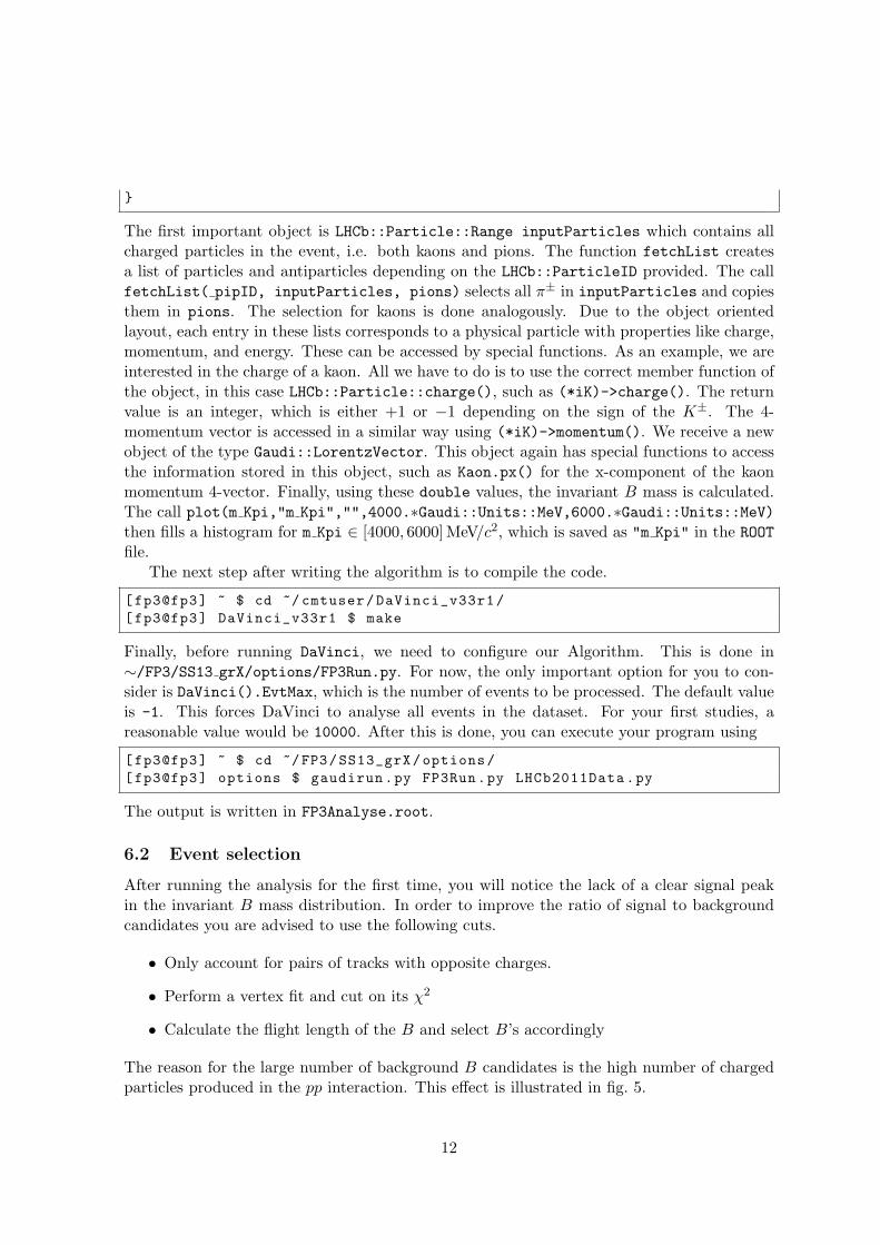
The first important object is LHCb::Particle::Range inputParticles which contains allcharged particles in the event, i.e. both kaons and pions. The function fetchList createsa list of particles and antiparticles depending on the LHCb::ParticleID provided. The callfetchList( pipID, inputParticles, pions) selects all π± in inputParticles and copiesthem in pions. The selection for kaons is done analogously. Due to the object orientedlayout, each entry in these lists corresponds to a physical particle with properties like charge,momentum, and energy. These can be accessed by special functions. As an example, we areinterested in the charge of a kaon. All we have to do is to use the correct member function ofthe object, in this case LHCb::Particle::charge(), such as (*iK)->charge(). The returnvalue is an integer, which is either +1 or −1 depending on the sign of the K±. The 4-momentum vector is accessed in a similar way using (*iK)->momentum(). We receive a newobject of the type Gaudi::LorentzVector. This object again has special functions to accessthe information stored in this object, such as Kaon.px() for the x-component of the kaonmomentum 4-vector. Finally, using these double values, the invariant B mass is calculated.The call plot(m Kpi,"m Kpi","",4000.∗Gaudi::Units::MeV,6000.∗Gaudi::Units::MeV)then fills a histogram for m Kpi ∈ [4000, 6000] MeV/c2, which is saved as "m Kpi" in the ROOTfile.

The next step after writing the algorithm is to compile the code.

[fp3@fp3] ~ $ cd ~/ cmtuser/DaVinci_v33r1/[fp3@fp3] DaVinci_v33r1 $ make

Finally, before running DaVinci, we need to configure our Algorithm. This is done in∼/FP3/SS13 grX/options/FP3Run.py. For now, the only important option for you to con-sider is DaVinci().EvtMax, which is the number of events to be processed. The default valueis -1. This forces DaVinci to analyse all events in the dataset. For your first studies, areasonable value would be 10000. After this is done, you can execute your program using

[fp3@fp3] ~ $ cd ~/FP3/SS13_grX/options/[fp3@fp3] options $ gaudirun.py FP3Run.py LHCb2011Data.py

The output is written in FP3Analyse.root.

6.2 Event selection

After running the analysis for the first time, you will notice the lack of a clear signal peakin the invariant B mass distribution. In order to improve the ratio of signal to backgroundcandidates you are advised to use the following cuts.

• Only account for pairs of tracks with opposite charges.

• Perform a vertex fit and cut on its χ2

• Calculate the flight length of the B and select B’s accordingly

The reason for the large number of background B candidates is the high number of chargedparticles produced in the pp interaction. This effect is illustrated in fig. 5.

12

Figure 5: Event display for the semileptonic decay B+→D0(→π+π−)µ+(ν)

Selecting three charged tracks out of one hundred and combining them to a new particleallows for about 105 combinations. Even the requirement for the combinations’ invariantmass to be compatible with the B mass leaves a high number of background candidates. Itis therefore necessary to apply additional selection criteria to enhance the ratio of signal tobackground candidates.

Using the knowledge of the decay B0→K−π+ allows to reduce the number of backgroundevents. A first choice is to check for the correct charge combination, i.e. to only use trackswith opposite charges. The next step is to take advantage of the relative long lifetime of theB mesons of 1.5 ps. Due to the high boost of the B meson system in the LHCb detector,the B decay vertex is displaced by several mm from the primary vertex, the pp interaction.The vertex position is obtained in a vertex fit. The K and π tracks are forced to have thesame origin, i.e. the B decay vertex. Using the quality of this fit allows to separate signalcombinations from random Kπ combinations. Most Kπ combinations still have the sameorigin, the pp primary vertex. Requiring a minimum distance between the B vertex and thepp interaction point allows to select true B mesons and suppress combinations from the ppcollision.

The vertex fit is performed by the vertexFitter() tool. The first step is to create theVertex object and the new Particle.

LHCb:: Vertex VtxTwoBody;LHCb:: Particle B0;B0.setParticleID( ( (*iK)->charge () > 0 ? _BID : _BbarID ) );

and then performing the fit

StatusCode scFit = vertexFitter()->fit (*(*iK),*(*ipi),VtxTwoBody , B0);

It is then possible to check the quality of the fit

13

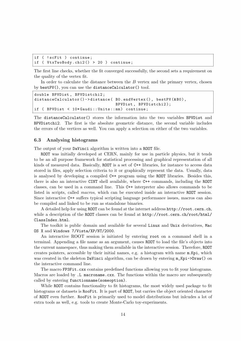
if ( !scFit ) continue;if ( VtxTwoBody.chi2() > 20 ) continue;

The first line checks, whether the fit converged successfully, the second sets a requirement onthe quality of the vertex fit.

In order to calculate the distance between the B vertex and the primary vertex, chosenby bestPV(), you can use the distanceCalculator() tool.

double BPVDist , BPVDistchi2;distanceCalculator ()->distance( B0.endVertex (), bestPV (&B0),

BPVDist , BPVDistchi2 );if ( BPVDist < 10* Gaudi:: Units::mm) continue;

The distanceCalculator() stores the information into the two variables BPVDist andBPVDistchi2. The first is the absolute geometric distance, the second variable includesthe errors of the vertices as well. You can apply a selection on either of the two variables.

6.3 Analysing histograms

The output of your DaVinci algorithm is written into a ROOT file.ROOT was initially developed at CERN, mainly for use in particle physics, but it tends

to be an all purpose framework for statistical processing and graphical representation of allkinds of measured data. Basically, ROOT is a set of C++ libraries, for instance to access datastored in files, apply selection criteria to it or graphically represent the data. Usually, datais analysed by developing a compiled C++ program using the ROOT libraries. Besides this,there is also an interactive CINT shell available, where C++ commands, including the ROOTclasses, can be used in a command line. This C++ interpreter also allows commands to belisted in scripts, called macros, which can be executed inside an interactive ROOT session.Since interactive C++ suffers typical scripting language performance issues, macros can alsobe compiled and linked to be run as standalone binaries.

A detailed help for using ROOT can be found at the internet address http://root.cern.ch,while a description of the ROOT classes can be found at http://root.cern.ch/root/html/ClassIndex.html.

The toolkit is public domain and available for several Linux and Unix derivatives, MacOS X and Windows 7/Vista/XP/NT/2000.

An interactive ROOT session is initiated by entering root on a command shell in aterminal. Appending a file name as an argument, causes ROOT to load the file’s objects intothe current namespace, thus making them available in the interactive session. Therefore, ROOTcreates pointers, accessible by their initial names, e.g. a histogram with name m Kpi, whichwas created in the skeleton DaVinci algorithm, can be drawn by entering m_Kpi->Draw() onthe interactive command line.

The macro FP3Fit.cxx contains predefined functions allowing you to fit your histograms.Macros are loaded by .L macroname.cxx. The functions within the macro are subsequentlycalled by entering functionname(someoption).

While ROOT contains functionality to fit histograms, the most widely used package to fithistograms or datasets is RooFit. It is part of ROOT, but carries the object oriented characterof ROOT even further. RooFit is primarily used to model distributions but inlcudes a lot ofextra tools as well, e.g. tools to create Monte-Carlo toy-experiments.

14

The object oriented structure mirrors the mathematics of variables and functions of vari-ables. Variables are represented by objects of type RooRealVar, probability density functions,henceforth referred to as p.d.f.s, by objects of type RooAbsPdf and data by objects of typeRooAbsData. Similar to mathematical function f(x|a, b) depending on the variable x and pa-rameters a and b, the corresponding RooAbsPdf objects depends on three RooRealVar objectsfor x, a, and b.

RooFit offers predefined types for commonly used function such as Gaussian p.d.f.(RooGaussian), n-th order polynomials (RooPolynomial), and the exponential p.d.f.(RooExponential). All of these are based on the abstract RooAbsPdf class.

6.3.1 Peaking background

After the selection, there still remain background events. There are two types of backgroundevents. The first are combinatorial background events. Those are smoothly distributed in theinvariant B mass. The other, however, are called peaking background events. These show asignature similar to the signal events. Typical events are similar B meson decays in whichone particle is misidentified. Such decays are B→K−K+ and B→π+π−. It is impossible tosuppress all of these events, so they have to be accounted for in the final fit. Other sources arerelated Bs decays. Due to the small mass difference between the B and Bs meson of about90 MeV/c2, the decay Bs→K−π+ also contributes to the signal peak. These contributionshave to be modeled and implemented in the final fit.

6.3.2 Usage of simulated events

It is common practise in particle physics to use simulated events to study the detector responseto certain event types and the resulting distributions, such as the invariant B mass.

In this exercise you will have to use four different samples of simulated events, B0→K−π+,Bs→K−π+, B→K−K+, and B→π+π−.

Using the simulation allows two things. First of all you can estimate the impact of thepeaking background compared to your signal, since you know how many events have beensimulated. On the other hand it allows to model the distributions.

Your task is to analyse these simulated events using the same algorithm you used before.You then have to find a parametrisation for the signal events B0 → K−π+ and its CPconjugated mode using RooFit as explained in the next section. You can then check, whetherit describes the LHCb data. You will find, that there are additional contributions to your Bpeak. These should come from the mentioned peaking background. In a similar way to theB0→K−π+ simulation, you can model the background events and check again, if your p.d.f.sdescribe the data.

Analysing different datasets requires no recompilation of your code, you simply use adifferent option file.

[fp3@fp3] ~ $ cd ~/FP3/SS13_grX/options/[fp3@fp3] options $ gaudirun.py FP3Run.py <someData >.py

The available datasets can be listed by

[fp3@fp3] ~ $ ls ~/FP3/SS13_grX/options/

15

It is also usefull to change the value of DaVinci().HistogramFile in FP3Run.py accordingto your dataset.

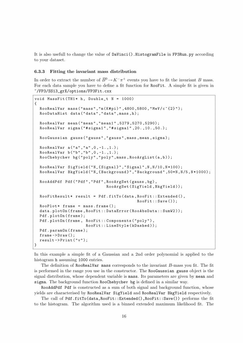
6.3.3 Fitting the invariant mass distribution

In order to extract the number of B0→K−π+ events you have to fit the invariant B mass.For each data sample you have to define a fit function for RooFit. A simple fit is given in~/FP3/SS13_grX/options/FP3Fit.cxx

void MassFit(TH1* h, Double_t N = 1000){

RooRealVar mass("mass","m(K#pi)" ,4800,5800,"MeV/c^{2}");RooDataHist data("data","data",mass ,h);

RooRealVar mean("mean","mean1" ,5279 ,5270 ,5290);RooRealVar sigma("#sigma1","#sigma1" ,20. ,10. ,50.);

RooGaussian gauss("gauss","gauss",mass ,mean ,sigma );

RooRealVar a("a","a" ,0,-1.,1.);RooRealVar b("b","b" ,0,-1.,1.);RooChebychev bg("poly","poly",mass ,RooArgList(a,b));

RooRealVar SigYield("N_{Signal}","Signal",N,N/10,N*100);RooRealVar BkgYield("N_{Background}","Background" ,50*N,N/5,N*1000);

RooAddPdf Pdf("Pdf","Pdf",RooArgSet(gauss ,bg),RooArgSet(SigYield ,BkgYield ));

RooFitResult* result = Pdf.fitTo(data ,RooFit :: Extended(),RooFit ::Save ());

RooPlot* frame = mass.frame ();data.plotOn(frame ,RooFit :: DataError(RooAbsData :: SumW2 ));Pdf.plotOn(frame);Pdf.plotOn(frame , RooFit :: Components("poly"),

RooFit :: LineStyle(kDashed ));Pdf.paramOn(frame);frame ->Draw ();result ->Print("v");

}

In this example a simple fit of a Gaussian and a 2nd order polynomial is applied to thehistogram h assuming 1000 entries.

The definition of RooRealVar mass corresponds to the invariant B-mass you fit. The fitis performed in the range you use in the constructor. The RooGaussian gauss object is thesignal distribution, whose dependent variable is mass. Its parameters are given by mean andsigma. The background function RooChebychev bg is defined in a similar way.

RooAddPdf Pdf is constructed as a sum of both signal and background function, whoseyields are characterised by RooRealVar SigYield and RooRealVar BkgYield respectively.

The call of Pdf.fitTo(data,RooFit::Extended(),RooFit::Save()) performs the fitto the histogram. The algorithm used is a binned extended maximum likelihood fit. The

16

remaining lines plot the output of the fit.This simple function can be used to determine the shape of B0→K−π+, Bs→K−π+,

B → K−K+, and B → π+π− decays using Monte Carlo simulations. In the final fit, youhave to expand the function to take all background contributions into account. You canconstruct the final p.d.f. using a new RooAddPdf. You have to fix the shape parameters forall contributions by using the RooRealVar::setConstant(kTRUE) function. In the final fitonly the yields and the shape of the combinatorial background are left floating.

6.3.4 Calculate the CP asymmetry

After having determined the shapes, you have to divide your sample into a B0→K−π+ anda B0→K+π− sample and perform the final fit in each sample. Using the signal yields youthen calculate the raw CP asymmetry

ARawCP

(B0→Kπ

)=N(B0→K−π+

)−N (B0→K+π−)

N(B0→K−π+

)+N (B0→K+π−)

. (16)

The raw asymmetry calculated from the fit to the invariant mass spectra does not includeeffects that may affect the CP asymmetry. These effects have to be considered in order todetermine the physical asymmetry ACP . Such effects are, for example, the production asym-metry, which leads to different production rates for B and B, and the detection asymmetrywhich takes into accout that there are different detection efficiencies for K+π− and π+K−.They are considered in the next equation

ACP(B0→Kπ

)= ARaw

CP

(B0→Kπ

)−AD(Kπ)− κdAP (B0) (17)

= ARawCP

(B0→Kπ

)+Acorr , (18)

where AD(Kπ) is the instrumental charge asymmetry, AP (B0) the production asymmetryand κd a decay time dependent correction factor.

The term AD(Kπ) needs to be accounted for due to the different interactions of particlesand anti-particles with the detector components. Another factor is the different behavior ofKaons and Pions in the detector. This systematic shift in ARaw

CP was thoroughly investigatedby the LHCb collaboration with very high statistics samples containing D0→K−π+ decays.

The production asymmetry for B and B mesons and defined as

AP =NB −NB

NB +NB, (19)

where NB and NB are the number of B and B events. In contrast to the B factories thetrue number of produced B mesons, as well as the ratio between B and B is not known atLHCb. The initial state violates CP , remind yourself that the LHC provides pp collisions.Furthermore, the bb jets produced need not both hadronize into a B meson. To investigatethis asymmetry it is necessary to count both B and B decays in a decay mode that is CPconserving. The decay B0→ J/ψK∗0 is used. There is only one Feynman diagram presentat leading order for this mode, so no CP violating interference is expected. The B factoriesproved this assumption to be correct. Additionally, with the K∗0 decaying into K+π−, it ispossible to determine the flavour of the B meson. The κd term is related to the efficiencyobserving an oscillation of the B or B, respectively.

Taking all these effects into account, the correction is given with Acorr = 0.7%.

17

References

[1] M. Kobayashi and T. Maskawa, Prog. Theor. Phys. 49 (1973) 652.

[2] L. -L. Chau and W. -Y. Keung, Phys. Rev. Lett. 53 (1984) 1802.

[3] H. Harari and M. Leurer, Phys. Lett. B 181 (1986) 123.

[4] L. Wolfenstein, Phys. Rev. Lett. 51 (1983) 1945.

[5] A. A. Alves, Jr. et al. [LHCb Collaboration], JINST 3 (2008) S08005.

18