Embed Size (px)
Citation preview

Measuring Leanness of Manufacturing Systems and Identifying Leanness Target by Considering Agility
Hung-da Wan
Dissertation submitted to the faculty of the Virginia Polytechnic Institute and State University
in partial fulfillment of the requirements for the degree of
Doctor of Philosophy in
Industrial and Systems Engineering
F. Frank Chen, Chair Subhash C. Sarin
Robert H. Sturges, Jr. Robert E. Taylor Philip Y. Huang
July 12, 2006 Blacksburg, Virginia
Keywords: Lean Manufacturing, Agile Manufacturing, Leanness, Agility, Data Envelopment Analysis (DEA), Slacks-Based Measure (SBM)
Copyright 2006, Hung-da Wan

Measuring Leanness of Manufacturing Systems and Identifying Leanness Target by Considering Agility
Hung-da Wan
Abstract
The implementation of lean manufacturing concepts has shown significant
impacts on various industries. Numerous tools and techniques have been developed to
tackle specific problems in order to eliminate wastes and carry out lean concepts. With
the focus on “how to make a system leaner,” little effort has been made on determining
“how lean the system is.” Lean assessment surveys evaluate the current status of a system
qualitatively against predefined lean indicators. Lean metrics are developed to quantify
performance of improvement initiatives, but each metric only focuses on one specific
area. Value Stream Maps demonstrate the current and future states graphically with the
emphasis on time-based performance only. A truly quantitative and synthesized measure
for overall leanness has not been established.
In some circumstances, being lean may not be the only goal for manufacturers. In
order to compete in the rapidly changing marketplace, manufacturing systems should also
be agile to respond quickly to uncertain demands. Nevertheless, being extremely agile
may increase the cost of regular operations and reduce the leanness of the system.
Similarly, being extremely lean may reduce flexibility and lower the agility level.
Therefore, a manufacturing system should be agile enough to handle the uncertainty of
demands and meanwhile be lean enough to deliver goods with competitive prices and
lead time. In order to achieve the appropriate leanness level, a leanness measure is needed
to address not only “how lean the system is” but also “how lean it should be.”
In this research, a methodology is proposed to quantitatively measure leanness
level of manufacturing systems using the Data Envelopment Analysis (DEA) technique.
The production process of each work piece is defined as a Decision Making Unit (DMU)
that transforms inputs of Cost and Time into output Value. Using a Slacks-Based Measure
(SBM) model, the DEA-Leanness Measure is developed to quantify the leanness level of
each DMU by comparing the DMU against the frontier of leanness. A Cost-Time-Value
analysis is developed to create virtual DMUs to push the frontier towards ideal leanness
so that an effective benchmark can be established. The DEA-Leanness Measure provides
a unit-invariant leanness score valued between 0 and 1, which is an indication of “how
lean the system is” and also “how much leaner the system can be.” With the help of Cost-
Time Profiling technique, directions of potential improvement can be identified by
comparing the profiles of DMUs with different leanness scores. The leanness measure
can also be weighted between Cost, Time and Value variables. The weighted DEA-
Leanness Measure provides a way to evaluate the impacts of improvement initiatives
with an emphasis on the company’s strategic focus.
Performing the DEA-Leanness measurement requires detailed cost and time data.
A Web-Based Kanban is developed to facilitate automated data collection and real-time
performance analysis. In some circumstances where detailed data is not readily available
but a Value Stream Maps (VSM) has been constructed, the applications of DEA-
Leanness Measure based on existing VSM are explored.
Besides pursuing leanness, satisfying a customer’s demand pattern requires
certain level of agility. Based on the DEA-Leanness Measure, appropriate leanness
targets can be identified for manufacturing systems considering sufficient agility level.
The Online-Delay and Offline-Delay Targets are determined to represent the minimum
acceptable delays considering inevitable waste within and beyond a manufacturing
system. Combining the two targets, a Lean-Agile Performance Index can then be derived
to evaluate if the system has achieved an appropriate level of leanness with sufficient
agility for meeting the customers’ demand.
Hypothetical cases mimicking real manufacturing systems are developed to verify
the proposed methodologies. An Excel-based DEA-Leanness Solver and a Web-Kanban
System have been developed to solve the mathematical models and to substantiate
potential applications of the leanness measure in real world. Finally, future research
directions are suggested to further enhance the results of this research.
iii
Acknowledgements
I want to express my deepest gratitude to my advisor, Dr. F. Frank Chen, for his
guidance on my research works and generous supports in all ways. I feel grateful for
having such a great advisor and knowing his loving family. I would like to thank all
professors on my advisory committee, Dr. Subhash C. Sarin, Dr. Robert H. Sturges, Dr.
Robert E. Taylor, and Dr. Philip Y. Huang, for continuously providing me insightful
comments and instructions and, especially, for their precious time and patience on the
extra long meetings throughout the steps of my Ph.D. program. Special thanks go to Dr.
Konstantinos P. Triantis, who taught me the Data Envelopment Analysis, which became
the core material of my dissertation. I also want to thank all other professors in the ISE
department for offering me the education and training that I need for professional life.
Especially, I deeply appreciate the Center for High Performance Manufacturing (CHPM)
for granting the full financial support on my research activities throughout the years.
The FMS Research Group led by Dr. Frank Chen has been a significant part of
my student life. All the group members and their families are literally my big family in
Blacksburg. The Babiceanu’s (Radu, Mihaela, and Laura), the Rivera’s (Leonardo, Ana,
and Camilo), Jiancheng Su and Yin He, Rami Musa, Dr. Hosang Jung, Liming Yao and
Jiming, and all former group members not only helped me in academic life but also gave
me the most joyful and memorable days in Virginia Tech. I would also like to thank
Guorong Huang, Shiyong Liu and many other friends from all over the world that I met
at Virginia Tech. Among them, the CSA members from my hometown, Taiwan, offered
the warmth of home, especially Jennifer Tsai, Jessie Tu, Eric Chia, Tony Ko, Yu-hsiu
Hung, and Ally Shen in the ISE department.
I cannot express enough thanks to my mother, father, sister, brother and other
family members in Taiwan for supporting my decision to come to the other end of the
world to study. Their caring concerns and warmest support are the endless thrusts for me
to move forward. Finally and most importantly, I would like to dedicate this dissertation
to my wife, Shu-yi Tsai, who fulfills the other half of my life. She is the reason for all
these to happen and be meaningful. I want to tell this to her everyday forever.
iv
Table of Contents
Abstract.............................................................................................................................. ii
Acknowledgements .......................................................................................................... iv
List of Figures................................................................................................................. viii
List of Tables ..................................................................................................................... x
List of Acronyms............................................................................................................. xii
Chapter 1 Introduction..................................................................................................... 1 1.1 Background and Motivation........................................................................................... 1
1.1.1 The Success and Limits of Lean Manufacturing .................................................................... 1 1.1.2 Enhancing Performance Based on Leanness and Agility ....................................................... 3
1.2 Problem Statement and Research Objectives................................................................. 4 1.2.1 Problem Statement.................................................................................................................. 4 1.2.2 Research Objectives and Scope .............................................................................................. 5
1.3 Framework of the Research ........................................................................................... 6 Chapter 2 Literature Review ........................................................................................... 8
2.1 Development of Lean and Agile Manufacturing Strategies........................................... 8 2.1.1 Lean Manufacturing ............................................................................................................... 8 2.1.2 Advantages and Limitations of Lean Manufacturing Implementation ................................. 12 2.1.3 Agile Manufacturing............................................................................................................. 15 2.1.4 Between Lean and Agile Strategies ...................................................................................... 18
2.2 Measuring Leanness..................................................................................................... 21 2.2.1 Leanness of Manufacturing Systems .................................................................................... 21 2.2.2 Qualitative Leanness Evaluation: Lean Assessment Approaches......................................... 22 2.2.3 Quantitative Leanness Evaluation: Lean Metrics ................................................................. 23 2.2.4 Graphical Leanness Evaluation: Value Stream Mapping ..................................................... 25
2.3 Data Envelopment Analysis (DEA) ............................................................................. 27 2.3.1 Overview of Data Envelopment Analysis............................................................................. 27 2.3.2 Mathematical Models of DEA.............................................................................................. 30 2.3.3 Measuring Leanness with DEA ............................................................................................ 32
2.4 Summarizing Literature of Leanness ........................................................................... 33 Chapter 3 DEA-Leanness Measure for Manufacturing Systems............................... 37
3.1 DEA-Leanness Measure .............................................................................................. 37 3.1.1 Decision Making Units (DMU) of DEA-Leanness Measure................................................ 37 3.1.2 Virtual DMUs and Leanness Frontier................................................................................... 40
v
3.1.3 Cost-Time-Value Analysis ................................................................................................... 43 3.2 DEA-Leanness based on Charnes-Cooper-Rhodes (CCR) Model............................... 46
3.2.1 Charnes-Cooper-Rhodes (CCR) Model................................................................................ 46 3.2.2 Hypothetical Cases Using CCR Model ................................................................................ 53 3.2.3 Weakness of CCR Model ..................................................................................................... 62
3.3 DEA-Leanness based on Slacks-Based Measure (SBM)............................................. 64 3.3.1 Slacks-Based Measure (SBM) Model................................................................................... 64 3.3.2 Hypothetical Cases Using SBM Model ................................................................................ 68
3.4 Contributions and Limitations of DEA-Leanness Measure ......................................... 73 Chapter 4 Extended Applications of DEA-Leanness Measure................................... 76
4.1 Tradeoffs between Competitive Strategies .................................................................. 76 4.1.1 Impacts of Improvement Initiatives...................................................................................... 77 4.1.2 Weighted DEA-Leanness Measure....................................................................................... 81
4.2 DEA-Leanness Measure based on Existing Value Stream Maps ................................ 88 4.2.1 DEA-Leanness for Manufacturing Systems Using VSM ..................................................... 89 4.2.2 DEA-Leanness Measure for Supply Chain........................................................................... 95
4.3 Identifying Potential Improvements Based on DEA-Leanness.................................... 99 4.3.1 Cost-Time Profile (CTP) Analysis ....................................................................................... 99 4.3.2 Improvement Cycle Based on DEA-Leanness and CTV Chart .......................................... 101
4.4 Rolling DEA Approach.............................................................................................. 103 Chapter 5 An Integrated Lean-Agile Performance Index ........................................ 108
5.1 Ultimate Leanness versus Acceptable Leanness Level.............................................. 108 5.2 Leanness Target Identification................................................................................... 110
5.2.1 Online-Delay Target ........................................................................................................... 111 5.2.2 Offline-Delay Target .......................................................................................................... 113 5.2.3 Lean-Agile Performance Target ......................................................................................... 117
5.3 Lean-Agile Performance Index.................................................................................. 118 5.4 Hypothetical Cases for Lean-Agile Targets ............................................................... 119
5.4.1 Case 4: Dedicated Flow Line with Imbalanced Workstations ............................................ 119 5.4.2 Case 5: Dedicated Flow Line with Fluctuating Demand .................................................... 124
Chapter 6 Software Implementation of DEA-Leanness Measure............................ 130 6.1 A Web-based Kanban System.................................................................................... 130
6.1.1 Background of Web-Kanban System Development ........................................................... 131 6.1.2 Framework and Functionality of Web-Kanban System...................................................... 133 6.1.3 Discussions on Web-Kanban System ................................................................................. 142
6.2 An Excel-based Solver for DEA-Leanness Measure ................................................. 143
vi

6.2.1 Framework and Functionality of Excel-based DEA-Leanness Solver................................ 144 6.2.2 Input and Output of Excel-based DEA-Leanness Solver.................................................... 146 6.2.3 Discussions on Excel-based DEA-Leanness Solver ........................................................... 150
Chapter 7 Conclusions.................................................................................................. 151 7.1 Summary and Conclusions......................................................................................... 151 7.2 Contributions of this Research................................................................................... 155 7.3 Future Research Areas ............................................................................................... 156
References...................................................................................................................... 159
Appendix A. Numerical Data of Hypothetical Cases................................................. 164
Appendix B. VBA Controller Program for Excel-based DEA-Leanness Solver .... 184
Vita ................................................................................................................................. 186
vii
List of Figures
Figure 1.1 Framework of Research..................................................................................... 7 Figure 2.1 DMU versus Technical Efficiency Frontier .................................................... 28 Figure 2.2 Three Elements of a Lean System................................................................... 35 Figure 3.1 Input and Output Variables of a DMU in DEA-Leanness Measure................ 39 Figure 3.2 DMUs with Various Conditions Mapped in Cost-Time-Value Space ............ 40 Figure 3.3 Pushing Frontier towards Ideal Leanness by Ideal DMUs.............................. 41 Figure 3.4 Pushing from the Empirical Frontier to the Ultimate Leanness ..................... 43 Figure 3.5 Cost-Time-Value Analysis for Creation of ADMUs and IDMUs.................. 44 Figure 3.6 Procedure of Cost Breakdown........................................................................ 46 Figure 3.7 CCR Model Scales the Input/Output Axis to Obtain the Efficiency Scores .. 48 Figure 3.8 CCR Scores Determined by Projecting to One Axis (2 Inputs with Same Level of Output)................................................................................................................ 49 Figure 3.9 CCR Scores Determined by Scaling Two Axes Simultaneously (2 Inputs with Same Level of Output)...................................................................................................... 49 Figure 3.10 Leanness Scores Obtained from CCR Model................................................ 51 Figure 3.11 Hypothetical Case: Dedicated Flow Line with Three Workstations ............. 53 Figure 3.12 ADMUs and IDMUs of Case 1 ..................................................................... 54 Figure 3.13 Leanness Scores of Case 1 Using CCR Model ............................................. 56 Figure 3.14 ADMUs and IDMUs of Case 2 ..................................................................... 58 Figure 3.15 Leanness Scores of Case 2 Using CCR Model ............................................. 59 Figure 3.16 ADMUs and IDMUs of Case 3 ..................................................................... 60 Figure 3.17 Leanness Scores of Case 3 Using CCR Model ............................................. 61 Figure 3.18 Slacks of Benchmark Undermine the Accuracy of CCR Scores................... 62 Figure 3.19 Slacks in SBM Model.................................................................................... 67 Figure 3.20 Leanness Scores of Case 1: SBM Model vs. CCR Model ............................ 69 Figure 3.21 Leanness Scores of Case 2: SBM Model vs. CCR Model ............................ 70 Figure 3.22 Leanness Scores of Case 3: SBM Model vs. CCR Model ............................ 72 Figure 4.1 Changes from Current State in terms of Cost and Time ................................. 77 Figure 4.2 DMUs Representing Current State and Eight Directions of Improvements ... 78 Figure 4.3 Leanness Scores of DMUs Representing Improvement Directions ................ 80 Figure 4.4 Weighted Leanness Scores with PT=2, PC=1 and PV=1 .................................. 86 Figure 4.5 Weighted Leanness Scores with PT=1, PC=2 and PV=1 .................................. 87 Figure 4.6 Weighted Leanness Scores with PT=1, PC=1 and PV=2 .................................. 87 Figure 4.7 Example Value Stream Map with Three Value-added Activities ................... 90 Figure 4.8 ADMU and IDMU Obtained from the VSM Example ................................... 92 Figure 4.9 An Example of VSM for Supply Chain .......................................................... 96 Figure 4.10 The DMUs from the VSM for Supply Chain ................................................ 98 Figure 4.11 The Components of a Cost-Time Profile..................................................... 100 Figure 4.12 Comparing DMUs in a CTV Chart ............................................................. 102 Figure 4.13 Improvement Cycle Based on Leanness Scores.......................................... 103 Figure 4.14 Frontiers Obtained from Different Data Sets .............................................. 104 Figure 4.15 The Concept of Rolling DEA Approach ..................................................... 105 Figure 5.1 Internal Delay and External Delay of a Lean Manufacturing System........... 109
viii
Figure 5.2 Timelines of Three Scenarios of a Two-Station Pull System........................ 112 Figure 5.3 Three Types of Offline Delays ...................................................................... 114 Figure 5.4 Identification of Lean-agile Performance Target DMU................................ 118 Figure 5.5 Graphical Evaluation of Lean-Agile Performance ........................................ 119 Figure 5.6 System Layout in Case 4 ............................................................................... 120 Figure 5.7 ADMUs and IDMUs of Case 4 ..................................................................... 121 Figure 5.8 Leanness Scores of Case 4 Using SBM Model ............................................. 122 Figure 5.9 Lean-Agile Target and Performance in Case 4 ............................................. 124 Figure 5.10 ADMUs and IDMUs in Case 5 ................................................................... 126 Figure 5.11 Leanness Scores of Case 5 .......................................................................... 127 Figure 5.12 Leanness Scores and Lean-agile Target in Case 5 ...................................... 129 Figure 6.1 Framework of Web-Kanban System ............................................................. 134 Figure 6.2 Interface of System Configuration Module: Material List ............................ 136 Figure 6.3 Interface of System Configuration Module: Order Placement...................... 137 Figure 6.4 Interface of Kanban Operating Module: Job List.......................................... 138 Figure 6.5 Interface of Kanban Operating Module: Job Processing Page...................... 139 Figure 6.6 Interface of Performance Monitoring Module: Kanban Tracking ................ 140 Figure 6.7 Interface of Performance Monitoring Module: WIP Level Monitoring........ 141 Figure 6.8 Interface of Performance Monitoring Module: Time-based Performance .... 141 Figure 6.9 Excel-based DEA-Leanness Solver: SBM Model......................................... 144 Figure 6.10 Excel-based DEA-Leanness Solver: SBM Model....................................... 145 Figure 6.11 Excel-based DEA-Leanness Solver: Input Data.......................................... 146 Figure 6.12 Excel-based DEA-Leanness Solver: ADMUs and IDMUs......................... 147 Figure 6.13 Excel-based DEA-Leanness Solver: Numerical Outputs ............................ 148 Figure 6.14 Excel-based DEA-Leanness Solver: Graphical Outputs ............................. 148 Figure 6.15 Excel-based DEA-Leanness Solver: Cost-Time Profile.............................. 149 Figure 6.16 Excel-based DEA-Leanness Solver: VA vs. NVA Costs............................ 149
ix
List of Tables
Table 2.1 Approaches to Achieving Leanness and Agility Simultaneously..................... 19 Table 2.2 An Example of Window Analysis with Relative Efficiency (%) ..................... 32 Table 3.1 Actual DMU (ADMU) vs. Ideally Lean DMU (IDMU) .................................. 41 Table 3.2 Reference Sets and Scores of DMUs................................................................ 52 Table 3.3 Costs Breakdown in Case 1 .............................................................................. 53 Table 3.4 Time Stamps of Case 1 ..................................................................................... 55 Table 3.5 Data and Results of Case 1 Using CCR Model ................................................ 56 Table 3.6 Time Stamps of Case 2 ..................................................................................... 57 Table 3.7 Data and Results of Case 2 Using CCR Model ................................................ 58 Table 3.8 Time Stamps of Case 3 ..................................................................................... 60 Table 3.9 Data and Results of Case 3 Using CCR Model ................................................ 61 Table 3.10 Current and Future Value Stream Maps Have Similar VA Times ................. 63 Table 3.11 Current and Future Value Stream Maps Have Similar VA Costs .................. 63 Table 3.12 Results of Case 1 Using SBM Model; Compared with CCR Model.............. 68 Table 3.13 Results of Case 2 Using SBM Model; Compared with CCR Model.............. 70 Table 3.14 Results of Case 3 Using SBM Model; Compared with CCR Model.............. 71 Table 4.1 Conditions for Leanness Improvements ........................................................... 78 Table 4.2 Leanness Scores of DMUs Representing Improvement Directions ................. 79 Table 4.3 Preparing Data for DEA-Leanness Measure based on Existing VSM ............. 92 Table 4.4 Leanness Score Derived from the VSM Example ............................................ 93 Table 4.5 ADMUs and IDMUs Obtained from a VSM for Supply Chain ....................... 97 Table 4.6 Leanness Score Derived from the VSM for Supply Chain............................... 98 Table 5.1 Cost and Time of the Online Delay Caused by Imbalances ........................... 113 Table 5.2 Cost and Time of the Offline Delay Caused by Batch Arrival....................... 115 Table 5.3 Cost and Time of the Offline Delay Caused by Batch Removal .................... 115 Table 5.4 Cost and Time of the Offline Delay Caused by Finished Goods Inventory ... 117 Table 5.5 Time Stamps of Case 4 ................................................................................... 121 Table 5.6 Data and Results of Case 4 Using SBM Model.............................................. 122 Table 5.7 Online-Delay Target in Case 4 ....................................................................... 123 Table 5.8 Lean-agile Target and Performance in Case 4................................................ 123 Table 5.9 Actual Demand, Inventory and Overtime of Case 5....................................... 126 Table 5.10 Summary of DEA-Leanness Measurement of Case 5 .................................. 126 Table 5.11 Offline Delay of Case 5 ................................................................................ 127 Table 5.12 Lean-agile Target and Performance in Case 5.............................................. 128 Table A.1 Time Stamps and Intervals of Case 1 ............................................................ 164 Table A.2 Costs of Value-Added Intervals of Case 1..................................................... 165 Table A.3 Costs of Non-Value-Added Intervals of Case 1 ............................................ 166 Table A.4 Time Stamps and Intervals of Case 2 ............................................................ 167 Table A.5 Costs of Value-Added Intervals of Case 2..................................................... 168 Table A.6 Costs of Non-Value-Added Intervals of Case 2 ............................................ 169 Table A.7 Time Stamps and Intervals of Case 3 ............................................................ 170 Table A.8 Costs of Value-Added Intervals of Case 3..................................................... 171 Table A.9 Costs of Non-Value-Added Intervals of Case 3 ............................................ 172
x
Table A.10 Time Stamps and Intervals of Case 4 .......................................................... 173 Table A.11 Costs of Value-Added Intervals of Case 4................................................... 174 Table A.12 Costs of Non-Value-Added Intervals of Case 4 .......................................... 175 Table A.13 Time Stamps and Intervals of Case 5: Day 1............................................... 176 Table A.14 Time Stamps and Intervals of Case 5: Day 2............................................... 177 Table A.15 Time Stamps and Intervals of Case 5: Day 3............................................... 178 Table A.16 Time Stamps and Intervals of Case 5: Day 4............................................... 179 Table A.17 Time Stamps and Intervals of Case 5: Day 5............................................... 180 Table A.18 ADMU and IDMU of Case 5: Day 1 to Day 2 ............................................ 181 Table A.19 ADMU and IDMU of Case 5: Day 3 to Day 4 ............................................ 182 Table A.20 ADMU and IDMU of Case 5: Day 5 ........................................................... 183
xi

List of Acronyms
ADMU Actual Decision Making Unit
BCC Model Banker-Charnes-Cooper Model
CCR Model Charnes-Cooper-Rhodes Model
CTP Cost-Time Profile
CTV Analysis Cost-Time-Value Analysis
CTV Chart Cost-Time-Value Chart
DEA Data Envelopment Analysis
DMU Decision Making Unit
IDMU Ideally Lean Decision Making Unit
ERP Enterprise Resources Planning
JIT Just-in-time Production
NVA Non-Value-Added
SBM Model Slacks-Based Measure Model
SME Small and Medium Enterprise
TPM Total Productive Maintenance
TPS Toyota Production System
VA Value-Added
VSM Value Stream Map
WIP Work-in-Process
xii
1.1 Background and Motivation
Chapter 1 Introduction
Many successful cases from various industries have demonstrated the
effectiveness of lean manufacturing concepts. The waste reduction and continuous
improvement techniques help lean practitioners pursue perfection. However, an effective
measure of the leanness level is absent. A measure of leanness is needed to provide
decision support information such as the current leanness level, the progress of lean
implementation, and the extent of potential improvements. In this research, a
methodology is proposed to measure the leanness level of manufacturing systems and to
identify the target of leanness level considering sufficient agility level. The background
information, motivation and an overview of this research are presented in this chapter.
1.1 Background and Motivation
While the efficiency and effectiveness of shop floor activities are continuously
improved by tools and techniques of lean manufacturing, a quantitative measure of the
leanness level to support the improvements has not been well developed. Without a
leanness measure, the leanness level of the current value stream is unknown, and the
improvement of leanness cannot be tracked. The success of lean manufacturing concepts
has urged the development of a leanness measure.
1.1.1 The Success and Limits of Lean Manufacturing
Ever since the research group in Massachusetts Institute of Technology (Womack
et al., 1990) started to promote the concepts of lean manufacturing in the 1990’s, the
“Lean Thinking” (Womack and Jones, 1996) has helped manufacturers improve their
performance by eliminating unnecessary activities in the manufacturing system from the
view point of customer defined value. Adapted from the Toyota Production System
(Ohno, 1988), lean thinking helps manufacturers identify various types of Waste, such as
waiting and overproduction, which were once acceptable to the Mass Production strategy.
By the efforts of eliminating theses wastes, materials can flow through the system
smoothly, and consequently, less resources are required to perform the manufacturing
1
1.1 Background and Motivation
tasks. The waste reduction efforts result in better performances, which typically include
lower cost, shorter lead time, more stable quality, lower work-in-process (WIP) and
inventory level, and increased product variety. Eventually, the benefits from
implementing lean concepts lead to a higher customer satisfaction level and, as a result,
better chance to survive and thrive in the global competition.
Various tools and techniques have been developed to identify and eliminate the
wastes in manufacturing systems. The mistake-proof techniques and continuous
improvement activities reinforce the advantages of lean implementation in the long run.
Each lean tool or technique usually focuses on solving a specific problem, such as high
work-in-process level, low availability of equipment, long setup time, etc. Therefore,
many of the tools are often applied simultaneously in order to improve the overall
leanness of a system. Performance metrics corresponding to the lean tools were
developed to track the improvements. Similarly, the lean metrics usually evaluates the
performance of a fraction of the overall leanness. Most of the time, a group of lean
metrics are used simultaneously to evaluate the effectiveness of the lean initiatives. An
integrated measure of leanness which is quantitative and objective is absent. Only by
reviewing a whole set of lean metrics, the lean practitioners can track the improvement in
each specific area and build a rough image of the overall leanness. The current level of
overall leanness is not measured, and the progress of improvement on overall leanness
cannot be tracked. As a result, lean practitioners know “how to improve the leanness” and
“what has been improved” but do not have the knowledge of “how lean the system is” or
“how much leaner it can become.” An integrated leanness measure should be developed
to guide the efforts of leanness improvements.
The benefits of implementing lean manufacturing concepts have been proven by
numerous lean practitioners reportedly. In addition to manufacturing activities, the impact
of lean thinking has been extended to other areas, such as service industries and
administrative sectors. It appears that the lean concepts can be effectively applied to all
activities in any system. However, empirical studies pointed out that the effectiveness of
lean implementation is limited when the contents of the activities are non-repetitive
(White and Prybutok, 2001). In other words, when the demand volume fluctuates, or
2

1.1 Background and Motivation
when the product types change frequently, the implementation of lean manufacturing
concepts becomes less beneficial.
Although the advantages are less significant, companies who do not have a stable
demand from customers can still apply the lean tools and techniques to lower the cost of
production, shorten the lead time, and stabilize the quality. Strategies for applying lean
principles in the environments of high product variety and low volumes have been
suggested by previous research (Jina et al., 1997). On the other hand, a different strategy,
Agile Manufacturing, has been developed to cope with the uncertainty of changing
demands (Goranson, 1999). The objective of an agile manufacturing system is to respond
swiftly to demand changes and gain the market before competitors can react. As a result,
the agile strategy is more advantageous than the lean manufacturing strategy in the
volatile, customer-driven environment.
1.1.2 Enhancing Performance Based on Leanness and Agility
Lean manufacturing and agile manufacturing strategies are both created to gain
advantage in the global competition, but the two solutions aim at different problems. The
major contribution of lean manufacturing is to improve efficiency, while the agile
strategy contributes mainly to responsiveness. Early research on agile manufacturing
argues that the agile strategy is an alternative to the well accepted lean strategy since the
market demand is increasingly more volatile. However, not all companies are targeting at
the extremely volatile or extremely stable market (Mason-Jones et al., 2000b). Most
organizations face a market that is between the two extremes. Being lean and agile at the
same time would be beneficial. Nevertheless, the two manufacturing strategies are not
fully compatible. Controversies are found in the objectives of the two strategies, e.g.,
lower unit cost versus higher flexibility. As a result, maximizing the agility of a system
may be harmful to the leanness, and vice versa (Goranson, 1999). A compromise between
lean and agile strategies would be more favorable in practice.
For different products and industries, different patterns of market demand can be
observed. For example, a demand can be categorized as steady, increasing, decreasing,
seasonal, or volatile. From a supplier’s point of view, the pattern of market demand is not
3
1.2 Problem Statement and Research Objectives
a controllable issue. The decision is either accepting the pattern or giving up the market.
Therefore, when a company is aiming at a certain market, the agility level required to
handle the uncertainty of the demand pattern has been defined by the market. In other
words, the preferred compromise between leanness and agility should be achieved by
maximizing the leanness level while a certain level of agility is maintained. Thus, a
supplier facing a stable demand should be as lean as possible while keeping minimal
level of agility. On the other hand, a supplier receiving custom orders frequently may
need to sacrifice its leanness to be highly agile. In order to achieve the balance between
leanness and agility, the decisions on performance improvement cannot be made only
based on “how lean the system is.” A methodology to decide “how lean the system should
be” also needs to be developed.
1.2 Problem Statement and Research Objectives
In this research, a methodology is developed to measure the leanness level of
manufacturing systems and identify the appropriate target of leanness. The objectives and
the framework of this research are presented in this section.
1.2.1 Problem Statement
While applying lean principles to a system, the progress and effectiveness of the
lean implementation are always the major concerns for decision makers. The following
three essential questions illustrate the decisions on lean implementation: “How lean is the
system?”, “How to become leaner?”, and, “How lean the system should be?”
Various tools and techniques have been developed to help lean practitioners
reduce wastes and enhance the leanness of the manufacturing system. The question, “how
to become leaner” has been answered by these lean tools and techniques. However, the
existing performance measures do not provide an explicit indication on how lean a
system is. Also, for the balance between leanness and agility, the target of appropriate
leanness level can not be identified or presented due to the absence of an effective
4
1.2 Problem Statement and Research Objectives
leanness measure. Therefore, the answers to how lean the system is” and “how lean the
system should be” are still absent.
In order to support the decisions made for lean implementation, a methodology
that identifies the leanness level of a system needs to be developed. The measurement of
leanness should be quantitative and objective, which can be applied on different systems
and can be compared between the systems. For a certain level of agility, a target of
appropriate leanness level needs to be identified. The leanness measure should be able to
present the leanness target in the same format as the leanness measure of current status so
that the lean practitioners can evaluate their performance by comparing the current
leanness level against the leanness target. The leanness measure and the target should
lead to improvement actions that can enhance leanness of the system in order to thrive in
the competitive market.
1.2.2 Research Objectives and Scope
The objective of this research is to develop a series of methodologies to help lean
practitioners ensure the effectiveness of the implementation of lean initiatives. Three
aspects of the objective are listed below.
1) Measuring Leanness of Manufacturing Systems: A leanness measure needs to
be developed that can quantify the leanness level of a manufacturing system to
provide an integrated index for “how lean the system is.”
2) Identifying Leanness Target: A leanness target needs to be identified that shows
the minimum of acceptable leanness level while maintaining sufficient agility.
The question “how lean the system should be” is answered by the leanness target.
3) Identifying Directions of Improvement: Directions of potential improvements
need to be identified to help the lean practitioners improve from current leanness
level to the leanness target. The concern of “How to achieve the leanness target”
is addressed by the improvement directions.
5
1.3 Framework of the Research
A methodology for leanness measurement and target identification is illustrated in
this research to carry out the three aspects of the research objective. Based on the context
of manufacturing systems, the proposed methodology is developed and verified. Due to
the availability of time and other resources, the scope of the research on leanness
measurement and target identification is limited to shop floor activities. A potential
application of the leanness measure on supply chain level is suggested, but it will be
verified in future research work. In the development of the methodology, existing
mathematical models for Data Envelopment Analysis (DEA) are adapted to develop the
measure of leanness scores. Computer programs are developed to solve the mathematical
models and substantiate practical applications of this methodology in real manufacturing
systems. Hypothetical cases of different scenarios are created to verify the effectiveness
of the proposed methodology. These cases depict the scenarios commonly found in real
manufacturing systems.
Although the scope of this research is limited to manufacturing systems, the
concepts of the leanness measurement and target identification can possibly be applied to
other circumstances. Potential extensions of the research scope include service industries,
administrative works, transportation industries, research and development sectors, etc.
The way to adapt and implement the proposed methodology in these circumstances is
beyond the current research.
1.3 Framework of the Research
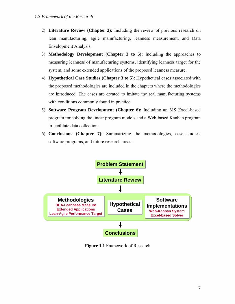
The dissertation is organized based on the framework of this research. Chapters
are developed to present the components of the framework, and the order of the chapters
corresponds to the timeline of the research activities. The components of this research are
listed as follows, and Figure 1.1 portrays the framework graphically.
1) Problem Statement (Chapter 1): Including background information, motivation,
objectives and scope of this research.
6
1.3 Framework of the Research
2) Literature Review (Chapter 2): Including the review of previous research on
lean manufacturing, agile manufacturing, leanness measurement, and Data
Envelopment Analysis.
3) Methodology Development (Chapter 3 to 5): Including the approaches to
measuring leanness of manufacturing systems, identifying leanness target for the
system, and some extended applications of the proposed leanness measure.
4) Hypothetical Case Studies (Chapter 3 to 5): Hypothetical cases associated with
the proposed methodologies are included in the chapters where the methodologies
are introduced. The cases are created to imitate the real manufacturing systems
with conditions commonly found in practice.
5) Software Program Development (Chapter 6): Including an MS Excel-based
program for solving the linear program models and a Web-based Kanban program
to facilitate data collection.
6) Conclusions (Chapter 7): Summarizing the methodologies, case studies,
software programs, and future research areas.
Problem StatementProblem Statement
Literature ReviewLiterature Review
MethodologiesDEA-Leanness MeasureExtended Applications
Lean-Agile Performance Target
MethodologiesDEA-Leanness MeasureExtended Applications
Lean-Agile Performance Target
HypotheticalCases
HypotheticalCases
SoftwareImplementations
Web-Kanban SystemExcel-based Solver
SoftwareImplementations
Web-Kanban SystemExcel-based Solver
ConclusionsConclusions
Figure 1.1 Framework of Research
7
2.1 Development of Lean and Agile Manufacturing Strategies
Chapter 2 Literature Review
In this chapter, previous research relevant to leanness measurement and target
identification is reviewed. First, the lean and agile manufacturing strategies are
introduced, and the relationship between lean and agile strategies is investigated.
Following that, previous research on leanness measurement is reviewed. The definition of
leanness is examined, and different ways to evaluate the leanness level are investigated.
After the review of leanness, the development of Data Envelopment Analysis (DEA) is
introduced, including the concepts, mathematical models and the modeling issues are
illustrated. Finally, a summary of the literature review wraps up this chapter.
2.1 Development of Lean and Agile Manufacturing Strategies
The lean and agile manufacturing strategies were both developed to make
manufacturing firms more competitive in the marketplace. However, conflicts exist
between the enablers of the two strategies. This section reviews the concepts of the two
strategies, the relationship between them, and the methodologies to be lean and agile
simultaneously.
2.1.1 Lean Manufacturing
The idea of conducting manufacturing processes in a lean manner is originated
from Toyota, the Japanese automaker that has been thriving in the global competition for
decades. In Toyota Production System, Ohno (1988) introduces the unique production
concepts developed in this company that helped them overcome difficult times since
World War II. In an environment lacking of resources, the Toyota Production System
(TPS), also known as Just-in-time (JIT) system, was developed to survive with minimum
amount of resources. The limited availability of resources made all mistakes unaffordable,
and reducing wastes in the shop floor became the mission of survival. When the oil crisis
struck the global economy in 1973, Toyota sustained and prospered because of the high
efficiency of the TPS. As a result, the lack of resources which was originally an obstacle
8
2.1 Development of Lean and Agile Manufacturing Strategies
to this company turned out to be the stepping stone for them to become a world-class
manufacturer.
In the 1980’s, a research group in MIT investigated the success of TPS. In
contrast to the mass production techniques inherited from Henry Ford almost a century
ago, the term “Lean Production” was coined to describe the highly efficient production
system which uses less of every resource to produce the same amount of products with
good quality. The findings of the investigations were summarized in The Machine that
Changed the World (Womack et al., 1990), which compares lean production with mass
production and points out several advantages and issues of becoming lean. This book
caught the attentions of manufacturers and researchers rapidly and popularized the
concept of lean manufacturing. Following that, Womack and Jones (1996) published the
book, Lean Thinking, which scrutinizes the concept of being lean. A vision of “lean
enterprise” was introduced by the authors that expanded the scope of implementing lean
principles to activities beyond the shop floor. It inspired later research, such as the lean
implementation in administrative work (William, 2003) and service sectors (Arbos, 2002).
More applications can be found in various environments which are beyond the scope of
this research.
The foundation of lean manufacturing is inherited from TPS. Ohno (1988) points
out that the basis of TPS is eliminating waste, and the two pillars supporting the system
are JIT and Autonomation. JIT implies a pull system where parts are moved only when
needed by the next process. Autonomation means “automation with human touch” which
prevents from producing defective parts when a mistake occurs or the machine fails. In
terms of waste, JIT eliminates the expected wastes caused by the design of the system.
On the other hand, Autonomation prevents the unexpected wastes caused by mistakes and
machine failures. Therefore, implementing JIT and Autonomation together eliminates the
two major aspects of waste in a manufacturing system. To realize the two concepts, all
wastes must be identified and eliminated. A “5 whys” procedure is used to find the root
cause of all wastes. The questions are driven by a philosophy that distinguishes TPS
from the others, which is to “rethink the common senses.” A well known result of the
“rethinking” is the finding that inventory, which was once considered as a tool to earn
more profit, is really a form of waste. Based on this philosophy, Ohno (1988) identifies
9
2.1 Development of Lean and Agile Manufacturing Strategies
seven types of wastes, which are listed as following, together with corresponding issues
identified by Feld (2000).
1) Waste of Overproduction: Excess Production – batch production, bottlenecks,
and curtain operations.
2) Waste of Time on Hand: Waiting – down time, part shortages, and long lead
time.
3) Waste in Transportation: Transportation – poor utilization of space, operator
travel distance, and material flow backtracking.
4) Waste of Processing Itself: Over Processing – redundant systems, misunderstood
quality requirements, poor process design.
5) Waste of Stock on Hand: Inventory – long changeover time, high raw material
inventory, high WIP, high finished goods inventory, and excessive management
decisions.
6) Waste of Movement: Motion – low productivity, multiple handling, and operator
idle time.
7) Waste of Making Defective Products: Defects – poor process yield, employee
turnover, low employee involvement, limited processing knowledge, and poor
communications.
In order to eliminate the seven types of wastes, revolutionary techniques were
developed in TPS. Ohno (1988) introduces the concepts of these techniques. Most of
them have become the fundamental techniques of lean manufacturing, including pull
system, Kanban, supermarket, demand leveling, flow, teamwork, multi-skilled worker,
small lot sizes, quick setup, mistake proof, and visual control. Monden (1998) illustrates
the details of all the tools and techniques used in TPS. Examples and instructions were
also provided which guide the readers through the implementation of a complete TPS. By
distinguishing the determinants of lean manufacturing, Detty and Yingling (2000)
summarize eight tenets for the philosophy of lean, which includes process stability,
standardized work, level production, just-in-time, quality-at-the-source, visual control,
production stop policy, and continuous improvement. Shah and Ward (2003) review 16
10
2.1 Development of Lean and Agile Manufacturing Strategies
key references of practices of lean manufacturing from 1977 to 1999. The “lean
practices,” which are the tools and techniques of lean implementation, are summarized
with the frequency of reference in the 16 papers. Among the 22 lean practices, the
JIT/continuous flow production, Pull system/Kanban, and Quick changeover techniques
were included in all 16 papers, and the Lot size reductions was referred 15 times out of 16.
The four lean practices appeared to be the most frequently implemented techniques for
lean implementation.
The vast number of tools or techniques included in TPS is an accumulation of
solutions over a long period. Every tool or technique was developed to solve a problem
and eliminate the waste found in Toyota’s production line, and it helps a manufacturing
system to become leaner in some aspects. However, for other companies, it is often
difficult to select a proper tool from the huge TPS tool box for their own problems. In
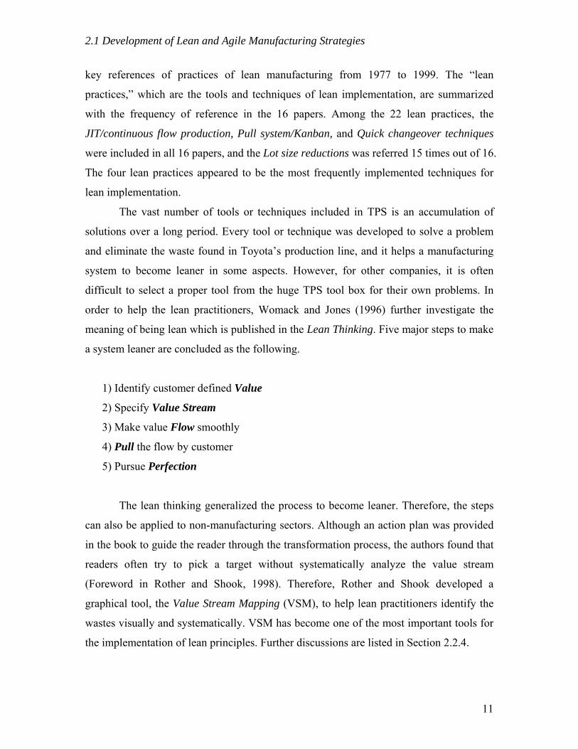
order to help the lean practitioners, Womack and Jones (1996) further investigate the
meaning of being lean which is published in the Lean Thinking. Five major steps to make
a system leaner are concluded as the following.
1) Identify customer defined Value
2) Specify Value Stream
3) Make value Flow smoothly
4) Pull the flow by customer
5) Pursue Perfection
The lean thinking generalized the process to become leaner. Therefore, the steps
can also be applied to non-manufacturing sectors. Although an action plan was provided
in the book to guide the reader through the transformation process, the authors found that
readers often try to pick a target without systematically analyze the value stream
(Foreword in Rother and Shook, 1998). Therefore, Rother and Shook developed a
graphical tool, the Value Stream Mapping (VSM), to help lean practitioners identify the
wastes visually and systematically. VSM has become one of the most important tools for
the implementation of lean principles. Further discussions are listed in Section 2.2.4.
11
2.1 Development of Lean and Agile Manufacturing Strategies
2.1.2 Advantages and Limitations of Lean Manufacturing Implementation
The purpose of implementing lean manufacturing is to become leaner. Ultimately,
the goal of a “leanest” manufacturing system is to become totally “waste-free.” Hopp and
Spearman (2000) introduce two statements on the waste-free state that were given as
early as 1983. The first statement used the term “zero inventories” to describe the ideally
lean state. Another statement described the ideal goal by “seven zeros” corresponding to
the different types of wastes. These are: zero defects, zero (excess) lot size, zero setups,
zero breakdowns, zero handling, zero lead time, and zero surging (i.e. smooth flow).
Hopp and Spearman pointed out that these “zeros” are physically unachievable in
practice, but the goals inspire an environment of continual improvement. Nevertheless,
the vision of the idea goals played an important role in developing the measure of
leanness, which is discussed in the next section.
Although the ideally lean state is typically not achievable, the waste-reduction
process of lean implementation helps manufacturers improve the efficiency and
effectiveness of the manufacturing activities. As shown in The Machine that Changed the
World (Womack, 1990), Toyota was able to assemble cars with shorter lead time and
lower defects rates using a smaller area and maintaining a significantly lower inventory
level when compared to GM in 1987. Many other cases have also shown that becoming
lean can enhance the competence of a manufacturing firm in the market place. One of the
key differences between lean and mass productions is the pull system, which prevents
most of the wastes from happening by blocking unnecessary activities. Sipper and Bulfen
(1997) point out that the major advantages of implementing pull system include:
1) Shorter lead time and hence higher flexibility to demand changes,
2) Reduced levels of inventory and other wastes,
3) Capacity considerations that are restricted by the system design, and
4) Inexpensive to implement.
Hopp and Spearman (2000) compare pull systems with traditional push systems in terms
of production planning and control:
12
2.1 Development of Lean and Agile Manufacturing Strategies
1) More Efficient: same throughput rate with less average WIP.
2) Easier to Control: rely on settings of easily observable WIP levels rather than
release rates.
3) More Robust: performance degrades much less than the push system by a
comparable percentage of error in release rate.
4) More Supportive of Improving Quality: the low WIP levels require high quality
to prevent from disruptions.
As to the overall advantages of implementing lean manufacturing, Callen et al. (2000)
carry out a plant-level cross-sectional analysis to analyze the performance of JIT and
non-JIT plants. Advantages of JIT plants against non-JIT plants are listed below.
1) Significantly less WIP and finished goods inventory.
2) Significantly lower variable cost and total cost.
3) Significantly more profitable.
4) JIT plants that adopted JIT earlier are more successful at reducing WIP,
minimizing costs, and maximizing profits.
5) JIT plants with better process quality are more successful in minimizing WIP and
finished goods inventories.
In general, the benefits from implementing lean concepts can be transferred into a
higher customer satisfaction level by providing products with lower cost, shorter lead
time, and more stable quality. Consequently, the lean practitioners can remain
competitive in the marketplace.
Despite of the advantages discussed above, a few drawbacks and limitations of
lean implementations were identified by previous research. First of all, the drawbacks of
becoming lean by implementing a pull system are pointed out by Sipper and Bulfen
(1997):
1) Myopic: Pull systems do not plan well for future events.
2) Reactive: Pull systems do not operate well under great variations of demand.
13

2.1 Development of Lean and Agile Manufacturing Strategies
3) Lack of Tracking: Pull systems cannot perform lot tracking, such as pegging a
lot for a customer.
As a result, the advantages of becoming lean are compromised when the demand
fluctuates and/or the number of custom orders increases. Furthermore, the types of
manufacturing systems are also factors that determine the effectiveness of lean
implementations. Several observations made by previous research are summarized as
follows.
1) For High Product Variety and Low Volumes (HVLV) Environment: Jina et al.
(1997) point out the difficulties to apply lean principles to HVLV environments.
Turbulence is the major cause of the difficulties. Four types of turbulence are
identified which cause the major impacts on lean implementation in HVLV
environments. They are the turbulences in schedule, product mix, volume, and
design.
2) For Repetitive and Non-repetitive Systems: White and Prybutok (2001)
conduct an empirical study on the relationship between lean practices and the type
of production systems. The findings of this research show that lean practices are
less likely to be implemented in the non-repetitive systems than in the repetitive
systems, although the benefits from implementing most of the lean practices do
not differ significantly between the two systems. The cause of the lower
implementation rate in non-repetitive systems was suggested by the authors that
the lean practices were designed in and have their roots in a repetitive production
system, namely Toyota.
3) For Small and Large Manufactures: Another empirical study conducted by
White et al. (1999) suggests that large manufacturers are more likely to
implement lean practices than small ones. Only the lean practice, multifunction
employee, is more likely to be implemented by small companies. The results also
show that the performance of both small and large manufacturers improved
significantly because of the lean implementation. Further investigations were
14
2.1 Development of Lean and Agile Manufacturing Strategies
suggested to help small firms to implement lean practices in order to compete
more successfully.
4) For Small and Medium Enterprises (SMEs): Ramaswamy et al. (2002)
investigate the issues of implementing lean practices in the SMEs. The results
suggest that buffer stock removal and lot size reduction are the most important
issues for SMEs, and the multifunctional workers and preventive maintenance are
least important. The authors pointed out a finding that the SMEs trying to
implement several lean initiatives simultaneously did not show remarkable
improvement over a period of time. Therefore, lacking of a well structured
implementation plan for SMEs may be the reason that lean practices are less
likely to be employed by SMEs.
Based on the review of past research, it can be concluded that the implementation
of lean manufacturing tools and techniques can bring forth remarkable improvements to
various type of manufacturing systems. However, the benefits are limited when the
demand changes dramatically in volume and product mix. Thus, the agile manufacturing
strategy was developed to complement the weakness of being lean.
2.1.3 Agile Manufacturing
The concept of Agile Manufacturing provides a different approach from lean
manufacturing to seeking for competence in the marketplace. While lean principles are
helping manufacturers to achieve lower cost, shorter lead time and better quality, it is
expected that the customers will want more. A common opinion shared by industry
leaders in the 1990’s was that the challenge of running business in the 21st century is to
provide high-quality, low-cost products, and “be responsive to customers’ specific unique
and rapidly changing needs” (Gunasekaran and Yusuf, 2002). Sanchez and Nagi (2001)
describe the context of the origin of agile manufacturing which initiated in 1991 as
follows. A report put together by a research group, the 21st Century Manufacturing
Enterprise Strategy, describes how US industrial competitiveness would evolve during
the next 15 years. Based on this effort, an Agile Manufacturing Enterprise Forum was
15
2.1 Development of Lean and Agile Manufacturing Strategies
formed at the Iacocca Institute at Lehigh University in 1991, which published the above
mentioned report and introduced the term “Agile Manufacturing” for the first time.
Katayama and Bennett (1990) state that the objective of agile manufacturing is to cope
with demand volatility by making changes in an economically viable and timely manner.
They also pointed out that the principles of agility are equally applicable to other sectors
of a business although the word “manufacturing” is used.
Unlike lean principles, agile manufacturing aims for unexpected situations. The
goal is to respond swiftly to demand changes and hence gain the market before
competitors can react (Goranson, 1999). Therefore, being agile is more advantageous
than being lean in terms of surviving in the volatile, customer-driven environment (Yusuf
and Adeleye, 2002). How agile a system can be is represented by the “agility.”
Gunasekaran and Yusuf (2002) review various definitions of agility given by previous
researchers and concluded that the agility in manufacturing system may be defined as:
The capability of an organization, by proactively establishing virtual manufacturing
with an efficient product development system, to (i) meet the changing market
requirements, (ii) maximize customer service level and (iii) minimize the cost of
goods, with an objective of being competitive in a global market and for an
increased chance of long-term survival and profit potential.
The authors further state that the agility must be supported by the flexibility of
people, processes and technologies. To achieve a high agility level, the system must focus
on strategic planning, product design, virtual enterprise, and automation and information
technology. Among the four enablers of agility, the Virtual Enterprise is a unique concept
that distinguishes agile manufacturing from the other strategies.
The formation of a virtual enterprise is based on temporary partnership between
companies or facilities. When a new demand appears, a virtual enterprise is formed with
a group of companies who are capable of handling the demand. When the demand is met,
the partnership is dismissed at the same time. It is an important technique to dramatically
increase the flexibility of a supply chain, and thus, enhance the agility. Goranson (1999)
introduce a framework of the Agile Virtual Enterprise together with a performance
16
2.1 Development of Lean and Agile Manufacturing Strategies
measurement model. Goldman et al. (1995) uses the term Virtual Organization to present
the importance of virtual partnership in agile manufacturing. Similar to the virtual
enterprise that is applied in the supply chain level, an approach named Virtual Cell was
developed to increase the agility of manufacturing systems in the shop floor level (Babu
et al., 2000; Baykasoglu, 2003).
Several measures to evaluate the level of agility have been proposed previous by
researchers. The measures can be categorized into three types.
1) Qualitative Assessment: Using survey questionnaires, the agility level is
evaluated by qualitatively assessing the performance of the system based on a set
of predefined agility indicators. Examples include the surveys developed by
Ramasesh et al. (2001) and Jackson and Johansson (2003). The assessment
approach evaluates how close the system is to the suggested agile guideline,
which may not be suitable for every system. Also, the result of qualitative survey
is subjective.
2) Attribute Measurement: The agility level is evaluated by measuring some of the
attributes of agility. Examples include the “sensitivity of productivity” used by
Helo (2004), and the “complexity index” developed by Arteta and Giachetti
(2004). This type of measure may be biased since the attribute may not be able to
fully represent the agility level. For example, increasing the complexity of a
system may cause unexpected situations and actually lower the agility level.
3) Target Fitness: The agility level is measured as the capability to change the
system in order to meet a set of potential situations. Examples include the
“reference model” developed by Goranson (1999), and the “state variable based
performance metrics” used by Sieger et al. (2000) This type of agility measure
needs a sophisticated methodology to determine the appropriate “targets” in order
to validate the measurement. However, since the targets are picked by the model
users, the measure may not be representing the real agility to cope with
unexpected situations.
17

2.1 Development of Lean and Agile Manufacturing Strategies
Beside of the issues associated with the three types of measures, Goranson (1999) points
out that agility may not be represented by a 0 to 1 scale which is commonly used by
performance metrics, such as efficiency and quality. The reason is that the absolute target
is not available. In other words, the state of 100% agile cannot be defined since product
variety and fluctuation of demand have no limit. As a result, no value obtained from an
agility measure can be interpreted correctly. Therefore, instead of trying to measure the
agility direction, it would be more reasonable to aim for an uncertainty level (i.e., the
demand pattern) and evaluate the capability to satisfy this demand agilely.
2.1.4 Between Lean and Agile Strategies
The relationship between lean and agile strategies has been intensely discussed by
researchers. As mentioned by Goranson (1999), some earlier researchers think that agile
and lean strategies are the same, while the other argue that agile manufacturing is an
advance of lean concepts. The author clarifies that the two strategies do have their
difference. Being too agile may harm the leanness of the system, while being too lean
could also reduce the agility level. Using an analogy to human body, Radnor and Boaden
(2004) utilize the word “anorexia” to describe the problem of a system that is too lean.
The corporate anorexia was referred to the inability to utilize or balance the
facets/resources of the organization effectively. The cause of the anorexia is being too
lean that the leanness level has gone beyond the “fitness” for the organization. In an
effort to develop a benchmark for lean initiatives, Comm and Mathaisel (2000) also point
out that the target of being lean is not “skinny or anorexic,” but that being lean is being
“fit.” In terms of lean and agile, the improvement efforts should aim at enough of agility
(leanness) while improving the other.
Mason-Jones et al. (2000a) summarize the distinguishing attributes of lean and
agile strategies concerning 11 aspects. Based on this summary, lean manufacturers
typically aims for predictable demands with low variety, long product lifecycle, and
lower profit margin. On the other hand, agile manufacturers demonstrate their core
competencies on volatile demand with high product variety, short product life cycle, and
higher profit margin. Similarly, Yusuf and Adeleye (2002) summarize the essential
18
2.1 Development of Lean and Agile Manufacturing Strategies
difference between lean and agile manufacturing based on 12 factors. Although conflicts
exist between the two strategies, researchers also point out that the two strategies are not
mutually exclusive (Aitken et al., 2002). Instead, they should be mutually supporting
(Katayama and Bennett, 1999). For manufacturing system in reality, the demand pattern
is normally neither extremely stable nor extremely volatile. In order to maximize the
competence, a manufacturing system should be benefited from both lean and agile
strategies. Different methodologies were developed to make a system lean and agile at
the same time. Three major approaches are listed in Table 2.1 with detailed discussions
following that.
Table 2.1 Approaches to Achieving Leanness and Agility Simultaneously
Approach Description
Virtual Group Applying Virtual Cells on functional layout
Safety Stock Balancing between inventories and disturbances
Leagile Supply Chain Positioning the decoupling point
The first methodology considers the flow of material. Prince and Kay (2003)
introduce the concept of virtual group to combine the lean and agile characteristics. The
virtual group is an application of virtual cells with functional layout. Similarly, other
research on virtual cells and virtual enterprises also inherits the characteristics of both
lean and agile strategies.
The second methodology to integrate lean and agile strategies is the use of safety
stock. Svensson (2003) investigate the relationship between companies’ inventories and
disturbances in logistics flow. It is suggested that the supply chains need to be agile while
striving to be lean. A balance between the inventories and disturbances is the objective,
but the approach to achieving the balance is not provided in this paper.
The third methodology is a “leagile” system that uses a decoupling point to
separate a supply chain into lean upstream section and agile downstream section. The
term “leagility” was first introduced by Naylor et al. (1999). In this paper, the meaning of
agility and leanness are reexamined, the function of a decoupling point in a supply chain
19
2.1 Development of Lean and Agile Manufacturing Strategies
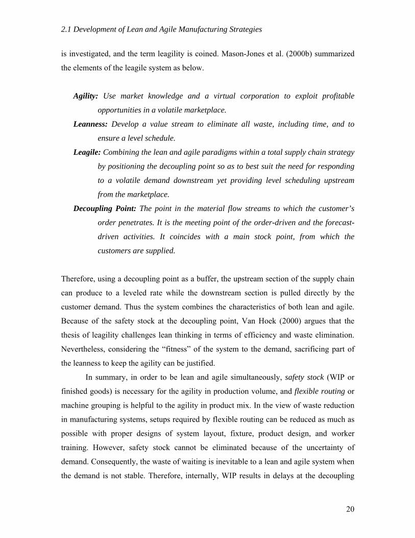
is investigated, and the term leagility is coined. Mason-Jones et al. (2000b) summarized
the elements of the leagile system as below.
Agility: Use market knowledge and a virtual corporation to exploit profitable
opportunities in a volatile marketplace.
Leanness: Develop a value stream to eliminate all waste, including time, and to
ensure a level schedule.
Leagile: Combining the lean and agile paradigms within a total supply chain strategy
by positioning the decoupling point so as to best suit the need for responding
to a volatile demand downstream yet providing level scheduling upstream
from the marketplace.
Decoupling Point: The point in the material flow streams to which the customer’s
order penetrates. It is the meeting point of the order-driven and the forecast-
driven activities. It coincides with a main stock point, from which the
customers are supplied.
Therefore, using a decoupling point as a buffer, the upstream section of the supply chain
can produce to a leveled rate while the downstream section is pulled directly by the
customer demand. Thus the system combines the characteristics of both lean and agile.
Because of the safety stock at the decoupling point, Van Hoek (2000) argues that the
thesis of leagility challenges lean thinking in terms of efficiency and waste elimination.
Nevertheless, considering the “fitness” of the system to the demand, sacrificing part of
the leanness to keep the agility can be justified.
In summary, in order to be lean and agile simultaneously, safety stock (WIP or
finished goods) is necessary for the agility in production volume, and flexible routing or
machine grouping is helpful to the agility in product mix. In the view of waste reduction
in manufacturing systems, setups required by flexible routing can be reduced as much as
possible with proper designs of system layout, fixture, product design, and worker
training. However, safety stock cannot be eliminated because of the uncertainty of
demand. Consequently, the waste of waiting is inevitable to a lean and agile system when
the demand is not stable. Therefore, internally, WIP results in delays at the decoupling
20

2.2 Measuring Leanness
point. Externally, finished goods inventory also results in delay. These observations form
the foundation for the proposed methodology of leanness target identification introduced
in Chapter 5.
2.2 Measuring Leanness
Numerous tools and techniques have been developed to eliminate wastes and
enhance leanness of manufacturing systems. However the needs to evaluate the level of
leanness did not receive comparable attention. Little effort was committed to the
development of leanness measures. A possible reason is that the meaning of leanness was
not well defined. This review starts with the definition of leanness of manufacturing
systems. After that, previous research on leanness measurement is reviewed in three
categories, namely Quantitative, Qualitative, and Graphical measures.
2.2.1 Leanness of Manufacturing Systems
The term Leanness has been used by several researchers while discussing on lean
manufacturing. However, the perceptions of leanness found in the literatures differ from
one author to another. Their opinions are reviewed in this section.
A definition of leanness is given by Naylor et al. (1999) while introducing the
concept of “leagility.” As shown in Section 2.1.4, “leanness” was used to describe a
process of implementing lean principles. This definition was quoted several times by the
proponents of leagility (Christopher and Towill, 2000; Mason-Jones et al., 2000a and
2000b; Towill and Christopher, 2002). Comm and Mathaisel (2000) describe leanness as
a relative measure of whether a company is “lean” or not. They also stated that “leanness
is a philosophy intended to significantly reduce cost and cycle time throughout the entire
value chain while continuing to improve product performance.” The term “total leanness”
was used by McIvor (2001) to imply a perfectly lean state of several key dimensions of
lean supply. The definition of leanness was not stated explicitly. Soriano-Meier and
Forrester (2002) develop a model to evaluate the degree of leanness of manufacturing
firms. In the model, the “Degree of Leanness” is the mean value of nine variables
21
2.2 Measuring Leanness
suggested by Karlsson and Ahlstrom (1996). The nine variables are developed to assess
the changes toward lean production, and the degree of leanness assesses the adoption of
lean production practices concerned with work organization in the production and
operation function. Finally, Radnor and Boaden (2004) attempted to outline the concept
of leanness by reviewing the previous uses of the word. In the review, “leanness” is
interpreted as an ideal state of lean, a context-dependent process, an ideal to be pursued, a
condition of being lean, a particular state of the relationships between the facets of a
system, or a journey to the ideal. A definition of leanness was not concluded in this paper,
and the attempt to outline the concept of leanness led to confusion because of the
diversity the various interpretations.
In summary, the meaning of leanness was interpreted in various ways by previous
researchers. One finding from the review is that the terms “leanness level” or “degree of
leanness” are used more often than “leanness” itself. Since the leanness of a system can
be represented as levels, a reasonable conclusion of the diversified opinions is that
“leanness level” is the state of a system which is in the range between the worst and
perfect. Therefore, the leanness level of a system can be defined and measured by
comparing the current state with the worst case and the perfect case. Thus, the level of
leanness can be quantified.
2.2.2 Qualitative Leanness Evaluation: Lean Assessment Approaches
Various lean assessment surveys have been suggested by the books that guide
readers through the implementation of lean manufacturing (Connor, 2001; Feld, 2000;
Jordan et al., 2001). The surveys are used to help the readers evaluate the degree of
adoption of the lean principles. Results of the surveys are often shown as scores
presenting the differences between the current state of the system and the ideal conditions
predefined in the surveys.
Scores obtained by the surveys provide an overview of the level of leanness and
indicate the percentages of completion of the suggested lean indicators. However, the
predefined lean indicators may not be appropriate for every system. The leanness score
obtained from a survey is only an evaluation of the compliance between the system and
22
2.2 Measuring Leanness
the lean indicators, instead of a quantitative score representing the real level of leanness.
Besides, the responses to the questionnaire are inevitably subjective. The results of the
surveys could be biased.
A dynamic assessment approach proposed by Wan and Chen (2006b) applies
different templates of lean indicators to different systems adaptively. The dynamic
assessment approach evaluates leanness level of a system based on a set of lean indicators
that are suitable for the system. A web-based tool is developed to perform the selection of
templates and the lean assessment. Leanness scores and improvement suggestions are
generated after the survey is completed. One difficulty of carrying out this approach is
that a large amount of templates for various environments need to be developed and
updated continuously. This weakness limits the effectiveness of this approach.
Beside the lean assessment surveys suggested by books for lean implementation,
there is an assessment model developed by Karlsson and Ahlstrom (1996) to assess the
changes of a system towards lean production. Nine groups of “measurable determinants”
were employed to measure the progress of lean implementation. Based on this model,
Soriano-Meier and Forrester (2002) proposes another model to evaluate the degree of
leanness of manufacturing firms. Similar to the previous models, this model evaluates the
“Degree of Adoption” of nine variables of leanness to be the leanness score.
Sanchez and Perez (2001) further developed a check-list of 36 lean indicators in
six groups to assess the changes towards lean. Although the indicators or determinants
were designed for qualitative evaluation, the survey type assessment is inevitably
subjective and still provides only rough estimates of the characteristics of leanness.
Furthermore, the suggested lean principles, indicators, and determinants are not
necessarily the best choices for various industries, and they may be outdated when
technology or management techniques advance dramatically.
2.2.3 Quantitative Leanness Evaluation: Lean Metrics
Lean metrics are the performance measures that are used to track the effectiveness
of lean implementation or continuous improvement. Allen et al. (2001) summarize a
collection of lean metrics categorized in four major groups, i.e., Productivity, Quality,
23
2.2 Measuring Leanness
Cost, and Safety. In each group, several lean metrics are suggested, such as “changeover
time” in Productivity, “yield and “scrap” in Quality, “material” and “labor” in Cost, and
“injuries” in Safety. Usually, a group of lean metrics are applied simultaneously. Each
metric is developed to evaluate the progress of improvement in a specific area. In other
words, a lean metric measures only a fraction of the overall leanness. A group of lean
metrics may be able to outline the overall leanness, but appropriate metrics must be
selected and synthesized into an integrated indicator of leanness. The Balanced Scorecard
(BSC) developed by Kaplan and Norton (1992) is a common method to select and
synthesize the performance measures for the decision making on improvements.
However, the scores provided by BSC indicate the progress of improvements instead of
leanness, and the target of full score changes when the BSC is reviewed. Therefore, a
benchmark for each lean metric or for the synthesized measure is needed if the level of
leanness is measured using the lean metrics.
Among the existing lean metrics, a measure of Manufacturing Cycle Efficiency
(MCE) was introduced as a lean metric for cycle time reduction (Levinson and Rerick,
2002). The MCE compares value-adding time with total cycle time to show the
efficiency of a manufacturing process.
TimeCycleTotalTimeaddingValueMCE −
=
This metric is commonly used by lean practitioners to get a picture of how lean a
manufacturing cycle is in terms of time efficiency. A MCE scored under 5% is not
uncommon, which urges lean practitioners to perform setup reduction. However, the
MCE cannot fully represent the leanness of the process because of two reasons. The first
reason is that MCE only considers time efficiency. Wastes occurred on other resources
were not included. The other reason is that the traditional MCE measure can be
misleading. Fogarty (1992) points out that MCE grossly overestimates manufacturing
efficiency because it measures the VA time in batches without considering the waiting
time of individual work piece. An alternative measure, the Value Added Efficiency (VAE),
was introduced to correct this problem. The VAE is calculated by dividing the processing
24

2.2 Measuring Leanness
(VA) time of a work piece by the manufacturing lead time for that work piece. The result
of this modification reinforced the needs to reduce the wastes in the manufacturing
processes. Although the VAE still lacks attention on the wastes of other resources, the
powerful concept of VAE becomes a foundation for the proposed methodology of
leanness measurement.
Beside of the lean performance metrics, Katayama and Bennett (1999) point out
that “labour productivity” was once used as a measure of leanness. It was argued that this
measure could mislead the decision makers to over invest on automation and ignore the
other benefits of leanness. However, the paper did not offer a substitute for the measure
of leanness. In a research of manufacturing competitiveness, Leung and Lee (2004)
identify “operation leanness” and “new-value creativeness” as the two principal
competencies of manufacturing firms. The operational leanness is defined as the
“performance” reflecting the competencies of a manufacturing firm by “utilizing its input
in more efficient ways.” The way to achieve “operation leanness” is to eliminate wastes
from the system. The seven types of wastes in TPS are categorized into three principal
types of wastes to be eliminated. Yet, no quantitative measure of leanness was presented
in the paper.
In summary, an effective measure that can quantify the level of leanness has not
been developed. A leanness measure is needed which can synthesize the various aspects
of the overall leanness into an integrated measure. Also, a benchmarking methodology is
needed to derive a meaningful value that represents the level of leanness.
2.2.4 Graphical Leanness Evaluation: Value Stream Mapping
Value Stream Mapping (VSM) is a graphical tool that maps out the process of a
system with a selected granulation in a selected scope. The tool was developed by Rother
and Shook (1998) and published in the book Learning to See. The tool itself does not
provide a quantitative measure of the level of leanness. Instead, the graphical
representation of the manufacturing processes visualized the value-adding activities and
wastes in the system. As stated by the authors:
25
2.2 Measuring Leanness
“It is much more useful than quantitative tools and layout diagrams that produce a
tally of non-value-added steps, lead time, distance traveled, the amount of
inventory, and so on. The VSM is a qualitative tool by which you describe in
detail how your facility should operate in order to create flow. Numbers are good
for creating a sense of urgency or as before/after measures. Value stream
mapping is good for describing what you are actually going to do to affect those
numbers.”
A current VSM and a future VSM are generated when an improvement project
starts. The current VSM graphically shows the level of leanness of the current system,
and the future VSM, serving as a target of improvement, is the benchmark of the leanness
level. By comparing the maps of the two stages, it can provide answers to the questions
“how lean is our system” and “how lean can it be”. From there, improvement tactics can
be made to guide the actions to reduce wastes and change the system toward the proposed
future state. The maps are reviewed periodically to track the progress of improvement
and determine whether the two maps need to be redrawn.
In Learning to See, a sample case of manufacturing system is used to illustrate the
procedures of creating the maps. Duggan (2002) introduces detailed procedures to apply
the VSM on mixed model production. In fact, the VSM has the potential to be applied to
various types of value streams, including non-manufacturing systems. As long as the
inputs/outputs and the internal processes of a system can be defined, the VSM technique
can be applied.
In the sense of leanness measurement, VSM does not provide a synthesized
quantitative measure like the lean assessment or lean metrics. To compliment this
weakness, Allen et al. (2001) develop a VSM Calibrate that shows the results of leanness
assessment on a radar chart. A current state calibrate and a future state calibrate are
generated based on the two stages of VSM. Thus, the gap between current state and
future state can be shown with measurements.
Since average numbers are employed to represent the time frames of the flow in
the value stream, the difference between individuals cannot be shown in the map. It
reduces the power of the VSM because the average numbers can deceive the real
26
2.3 Data Envelopment Analysis (DEA)
conditions and mislead the decision makers. Another weakness of the VSM is that “cost”
is not shown explicitly, since it is created strictly based on the time frames of the
processes. Although the other resources, such as material and labor, are included in the
map, it is difficult to identify the overall cost of a process merely from the map.
Therefore, complementary figures or tables must be provided if the VSM is used as a
representation of leanness level.
2.3 Data Envelopment Analysis (DEA)
In this research, a methodology is developed to measure the leanness level of
manufacturing systems. As discussed in previous sections, an effective measure of
leanness should be able to integrate the different aspects of the leanness, and a
benchmark need to be identified for the measure. The Data Envelopment Analysis (DEA)
is capable of analyzing multiple input/output variables and identifying a benchmark
based on each data set. With these features, the DEA model appears to be a suitable tool
for the leanness measurement. This section reviews the concepts and models of DEA.
Also, the issues of applying DEA in the leanness measurement are discussed.
2.3.1 Overview of Data Envelopment Analysis
Data Envelopment Analysis (DEA) is a methodology developed for performance
measurement. It identifies the best practices of Decision Making Units (DMU) and
determines the production frontier accordingly by solving a mathematical program based
on historical data. The concept and the mathematical model are first introduced by
Charnes et al. (1978). The production frontier identified by the model envelopes all
DMUs of the data set and serves as the performance benchmark for each DMU. The
efficiency of the DMU can then be evaluated by calculating the distance from the DMU
to its benchmark. The components of a DEA Model are listed below.
1) Decision Making Units (DMUs): objects of the observation
2) Input Variables: resources consumed by a DMU
27

2.3 Data Envelopment Analysis (DEA)
3) Output Variables: products or services delivered by a DMU
4) Transformation Processes: the procedure that transforms inputs into outputs
A simplest form of performance measure or efficiency is the ratio between output
and input (Boussofiane, 1991). When multiple inputs and outputs are considered
simultaneously, the efficiency measure can be formulated as:
Efficiency = Weighted sum of outputs
Weighted sum of inputs
Based on microeconomic theories, a system is more productive if it can produce more
output(s) with a same or less input level. Therefore, an Input-oriented DEA model
evaluates the inefficiency of a system based on the extent that the input variable(s) can
possibly be decreased while producing the same level of output(s). On the other hand, the
Output-oriented DEA model addresses the inefficiency of a system by determining the
extent that the output variable(s) can possibly be increased while using the same level of
input(s). The relationships between the efficient DMUs, inefficient DMUs, and the
Technical Efficiency Frontier are shown in Figure 2.1 with two different scenarios. Cases
with higher dimensions (more input/output variables) are difficult to be presented
graphically, but they can be solved by mathematical programs.
InputInput Input 1Input 1
OutputOutput Input 2Input 2
11--input, 1input, 1--outputoutput 22--input, 1input, 1--outputoutputTechnicalTechnicalEfficiencyEfficiencyFrontierFrontierEfficientEfficient
DMUsDMUs
IsoquantIsoquantEfficientEfficientDMUsDMUs
Figure 2.1 DMU versus Technical Efficiency Frontier
In the DEA model, the production frontier and efficiency scores are determined
using a mathematical that addresses the weighted multiple inputs and outputs. The
28
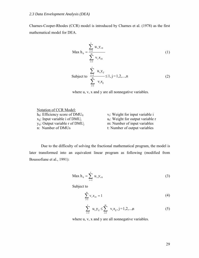
2.3 Data Envelopment Analysis (DEA)
Charnes-Cooper-Rhodes (CCR) model is introduced by Charnes et al. (1978) as the first
mathematical model for DEA.
∑
∑
=
== m
ii
t
rr
x
y
10i
10r
0
v
u hMax (1)
Subject to n1,2,...,=j1, v
u
i1
r1 ≤
∑
∑
=
=
ij
m
i
rj
t
r
x
y (2)
where u, v, x and y are all nonnegative variables.
Notation of CCR Model: h0: Efficiency score of DMU0xij: Input variable i of DMUjyrj: Output variable r of DMUj n: Number of DMUs
vi: Weight for input variable i ur: Weight for output variable r m: Number of input variables t: Number of output variables
Due to the difficulty of solving the fractional mathematical program, the model is
later transformed into an equivalent linear program as following (modified from
Boussofiane et al., 1991):
∑=
=t
rry
10r0 u hMax (3)
Subject to
1v1
0i =∑=
m
iix (4)
n1,2,...,=j , vu i1
r1
ij
m
irj
t
rxy ∑∑
==
≤ (5)
where u, v, x and y are all nonnegative variables.
29

2.3 Data Envelopment Analysis (DEA)
Thus, the DEA model can be solved by linear programming techniques, and the
frontier and the efficiency score of each DMU can be determined accordingly. In the
solution, the weights for the Input/Output variables of each DMU are derived by the DEA
model which maximizes the efficiency score of the unit. Therefore, the weights also
imply the sensitivities of the variables.
The empirical frontier determined by the DEA model is composed by the best
practices. The projection of each DMU on the frontier is either a best practice unit or a
linear combination of a set of best practice units. These best practice units are known as
peers or reference set of the DMUs. As a result, each DMU can be represented as a
convex combination of a set of peer DMUs, and the frontier “envelops” all the DMUs in
a convex hall. By analyzing the relationships between each DMU and its peers, the DEA
model determines the efficiency score of each DMU based on the distance to the
benchmark frontier. It also suggests realistic goals of efficiency in different aspects for
each DMU. The routes from the DMU to the goals of efficiency can be identified as the
potential improvements to reach the highest efficiency. Based on the directions of
potential improvements, decision makers can look into the details of the transformation
processes, so that the causes of inefficiency can be identified and avoided. Thus the
highest efficiency can be achieved in future practices.
The features of the basic DEA modeling are summarized below.
1) DEA evaluates “Efficiency” of previous operations without outsourcing for
benchmark.
2) DEA is capable of analyzing multiple input/output variables.
3) DEA provides “dimension-free” efficiency scores that can be easily compared.
2.3.2 Mathematical Models of DEA
The CCR model introduced in the previous section is the original model of DEA.
Two types of CCR model can be formulated based on the direction of improvement
(Cooper et al., 2000).
30
2.3 Data Envelopment Analysis (DEA)
Input-oriented CCR (CCR-I) model: aims at reducing the input amounts by as
much as possible while keeping at least the present output levels.
Output-oriented CCR (CCR-O) model: maximizes output levels under at most
the present input consumption.
Some other DEA models were developed for different situations. Cooper et al. (2000)
summarize the features of the models as follows.
Banker-Charnes-Cooper (BCC) Model: defines the production possibility set
by means of the existing DMUs and their convex hull. An efficiency
value is given which is not less than the CCR model.
Additive Models: deal with input excesses and output shortfalls simultaneously.
Slack-Based Measure (SBM) of efficiency: deals with the input excesses and
output shortfalls and use the Additive Model to give a scalar measure
ranging from 0 to 1 that encompasses all of the inefficiencies that the
model can identify.
Among the different models, BCC model can also have the options of either
Input-oriented or Output-oriented. The Additive Model and SBM Model encounter the
slacks in the linear program, which are the input excesses and output shortage. The
efficiency scores derived from CCR and BCC models does not encounter the slacks.
However when slacks exist, the actual efficiency is lower than the score. Therefore, when
the output results of a data set contains large amount of slacks, the Additive Model or the
SBM Model should be considered. More detailed discussions on the slacks can be found
in Section 3.2 and 3.3.
The DEA models compare all DMUs in a data set together to determine the
efficiency scores. It is considered as a static snap shot of the performances of DMUs in a
frozen time frame. In some cases, understanding the changes of the efficiency of a DMU
over time is more important. An approach to capturing the dynamics of the performances
of DMUs was proposed by Charnes et al. 1985. The “Window Analysis” approach
displays the efficiency scores of DMUs in “windows” of time frames. In each window,
31

2.3 Data Envelopment Analysis (DEA)
the performance of each DMU is traced for several consecutive periods of time.
Consequently, the performance of a DMU can be compared to other DMUs in each
period and meanwhile compared to itself over time. An example of window analysis is
listed in Table 2.2. The columns of the table represent the relative efficiency scores of
DMUs in each quarter. Each window compares the n branches in three consecutive
quarters. A window shifts to the next by adding a new quarter and dropping the earliest
quarter from the window. Therefore, the window analysis captures the changes of
efficiency over time.
Table 2.2 An Example of Window Analysis with Relative Efficiency (%) Week 1 2 3 4 5
Line 1 Window 1 51.3 60.2 64.1 Window 2 85.4 72.5 91.2 Window 3 83.7 100 78.6
Line 2 Window 1 93.5 92.6 100 Window 2 83.4 100 88.2 Window 3 95.4 70.7 85.5
Line 3 Window 1 100 80.0 74.9 Window 2 100 82.2 100 Window 3 93.2 85.7 100
2.3.3 Measuring Leanness with DEA
According to the literature review of leanness measurement, an effective measure
of leanness has not been developed. The measure must be able to synthesize the various
aspects of the overall leanness into an integrated measure. Also, an appropriate
benchmark for leanness is not always available. Furthermore, the technology frontier
changes continuously over time, and the benchmark needs to be updated accordingly.
With the features of DEA model, these difficulties can be resolved. Using the DEA
model to measure leanness, the benchmark can be identified from historical data and the
frontier can be updated whenever new observations become available. Therefore, DEA
appears to be a suitable tool for leanness measurement.
32

2.4 Summarizing Literature of Leanness
However, DEA determines the “best practices” (the DMUs forming the frontier)
as 100% efficient. Since practically no manufacturing system can perform the production
tasks without any waste, leanness level of the best practices can never reach 100%. The
efficiency score obtained by using DEA is not a reasonable measure for leanness
measurement. To adapt the DEA model into an appropriate measure of leanness, a virtual
frontier with 100% leanness needs to be identified. A methodology is developed in this
research to identify the appropriate leanness frontier and measure leanness level using
DEA model. Details of the modification of DEA approach are illustrated in Chapter 3.
In the review of the applications of DEA in leanness measurement, similar
adaptation of DEA approach has not been found. Typical applications of DEA such as
performance measurement and benchmarking a performance measure are still the major
role of DEA in the implementation of lean manufacturing. Only part of this research has
been publicly presented at the Annual Industrial Engineering Research Conference to
demonstrate the concept of measuring leanness with DEA, including the concept of
creating Ideal DMUs to obtain an appropriate frontier (Wan and Chen, 2005) and the
leanness measure based on SBM model (Wand and Chen, 2006a).
2.4 Summarizing Literature of Leanness
For lean practitioners, the desires to be able to evaluate the level of leanness
quantitatively and objectively are not successfully met. The assessment approach
commonly used in industry gives a vague impression of the current state of the system
based on “what lean initiatives have been applied” and “what other lean initiatives are
currently available.” A direct measure of leanness is not provided by using this approach.
Several lean metrics have been developed to quantitatively evaluate the performance of
lean implementation. However, each lean metric only evaluates a fraction of the overall
leanness. Moreover, such measurements often evaluate only the progress of improvement
without providing appropriate targets for the lean metrics. With the knowledge that
leanness should be improved without compromising the desired level of agility, the
continuous improvement efforts should aim for a target that does not harm the other
33
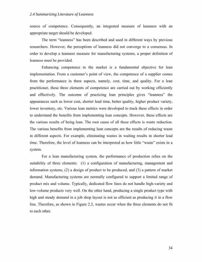
2.4 Summarizing Literature of Leanness
source of competence. Consequently, an integrated measure of leanness with an
appropriate target should be developed.
The term “leanness” has been described and used in different ways by previous
researchers. However, the perceptions of leanness did not converge to a consensus. In
order to develop a leanness measure for manufacturing systems, a proper definition of
leanness must be provided.
Enhancing competence in the market is a fundamental objective for lean
implementation. From a customer’s point of view, the competence of a supplier comes
from the performance in three aspects, namely, cost, time, and quality. For a lean
practitioner, these three elements of competence are carried out by working efficiently
and effectively. The outcome of practicing lean principles gives “leanness” the
appearances such as lower cost, shorter lead time, better quality, higher product variety,
lower inventory, etc. Various lean metrics were developed to track these effects in order
to understand the benefits from implementing lean concepts. However, these effects are
the various results of being lean. The root cause of all these effects is waste reduction.
The various benefits from implementing lean concepts are the results of reducing waste
in different aspects. For example, eliminating wastes in waiting results in shorter lead
time. Therefore, the level of leanness can be interpreted as how little “waste” exists in a
system.
For a lean manufacturing system, the performance of production relies on the
suitability of three elements: (1) a configuration of manufacturing, management and
information systems, (2) a design of product to be produced, and (3) a pattern of market
demand. Manufacturing systems are normally configured to support a limited range of
product mix and volume. Typically, dedicated flow lines do not handle high-variety and
low-volume products very well. On the other hand, producing a single product type with
high and steady demand in a job shop layout is not as efficient as producing it in a flow
line. Therefore, as shown in Figure 2.2, wastes occur when the three elements do not fit
to each other.
34
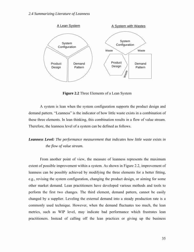
2.4 Summarizing Literature of Leanness
SystemConfigurationSystem
ConfigurationWaste Waste
Was
te
ProductDesign
DemandPattern
DemandPattern
ProductDesign
A Lean System A System with Wastes
Figure 2.2 Three Elements of a Lean System
A system is lean when the system configuration supports the product design and
demand pattern. “Leanness” is the indicator of how little waste exists in a combination of
these three elements. In lean thinking, this combination results in a flow of value stream.
Therefore, the leanness level of a system can be defined as follows.
Leanness Level: The performance measurement that indicates how little waste exists in
the flow of value stream.
From another point of view, the measure of leanness represents the maximum
extent of possible improvement within a system. As shown in Figure 2.2, improvement of
leanness can be possibly achieved by modifying the three elements for a better fitting,
e.g., revising the system configuration, changing the product design, or aiming for some
other market demand. Lean practitioners have developed various methods and tools to
perform the first two changes. The third element, demand pattern, cannot be easily
changed by a supplier. Leveling the external demand into a steady production rate is a
commonly used technique. However, when the demand fluctuates too much, the lean
metrics, such as WIP level, may indicate bad performance which frustrates lean
practitioners. Instead of calling off the lean practices or giving up the business
35

2.4 Summarizing Literature of Leanness
opportunity, a target of leanness level that considers the desired agility level to cope with
fluctuating demand should be developed.
36
3.1 DEA-Leanness Measure
Chapter 3 DEA-Leanness Measure for Manufacturing
Systems
In this chapter, a methodology using DEA technique is proposed for measuring
the leanness level of manufacturing systems. As discussed in Section 2.3, the
performance score derived from DEA is not equal to leanness score directly. Through a
Cost-Time-Value analysis, the DEA-Leanness measure creates virtual DMUs to push the
frontier towards an ideal state of leanness. Thus the benchmark for leanness score is
established. This methodology is explained in Section 3.1 in detail. Following that, two
mathematical models (i.e., CCR and SBM models introduced in Section 2.3) are
introduced to perform the computation of leanness scores. Due to a weakness of CCR
model, the SBM model delivers better results on the application of leanness measurement.
Hence, SBM model is selected as the core model of the DEA-Leanness Measure and is
employed in subsequent chapters.
3.1 DEA-Leanness Measure
In this section, a methodology combining DEA and Cost-Time-Value Analysis is
proposed for measuring leanness level of manufacturing systems. This methodology
consists of three major components: Actual DMUs, Virtual DMUs, and a Leanness
Frontier. The DEA-Leanness Measure uses virtual DMUs to push the frontier towards
ideal leanness in order to obtain a viable benchmark for leanness. Before the DEA-
Leanness Measure can be performed, the DMUs must be clearly defined.
3.1.1 Decision Making Units (DMU) of DEA-Leanness Measure
In Section 2.4, leanness level has been defined as the performance of the
production flow of a value stream. According to the lean concepts, the ideal case of lean
manufacturing is one-piece flow without interruption. Therefore, the leanness level of a
system can be measured as the performance of the flow of each work piece. In other
37
3.1 DEA-Leanness Measure
words, the DMU for DEA-Leanness should be defined as the work piece that flows
through the manufacturing system, and the leanness level of each DMU is calculated by
comparing the input-output ratio using the DEA models. Yet different systems or product
types consume different resources and deliver different functions or values to satisfy
customers. If the input/output variables need to be modified for different scenarios, the
leanness measure would not be user-friendly.
Considering the competitiveness in the marketplace, Cost, Time and Quality are
the three key performance measures for surviving and winning. Cost and Time are clearly
the input variables where decreasing the consumption of them improves the performance.
Since the consumption of all types of resources, such as material, labor or energy, can be
fully translated into values of cost and time, the two variables are perfect representations
for the inputs of the DEA-Leanness Measure. As to the output variable, the narrowly
defined Quality of a product does not cover other elements of output, such as service
level, customer satisfaction, or on-time delivery. Note that “on-time delivery” is not part
of the Time variable because it is the performance of meeting customer’s requirement
where early shipments are actually not welcomed. Actually, quality problems identified
within the manufacturing system lead to rework or scrap, which can be translated into
cost and time as input resources. In contrast, the quality problems found by customers
after the product are delivered do not increase the cost and time of the production process.
Instead, the price may be discounted to compensate the defects (if acceptable), or the
customer may express a low satisfaction rating on that product. In other words, a
defective product delivers lower Value to the customer than originally expected.
Johansson et al. (1993) proposes a “Total Value” metric as follows:
TimeLeadCostServiceQualityValueTotal
××
=
This ratio has been cited by researchers to represent a performance metric in terms of
“value to customers” (Naylor et al., 1999; Mason-Jones et al., 2000a). However, the Cost,
Time, and Internal Quality issues may not have any effect on a customer’s purchasing
experience directly. Instead, the factors that really affect the customer’s perception of
Value should be Price, On-time Delivery or Availability, After-sales Quality problems,
38
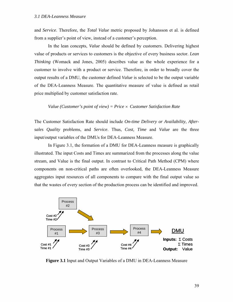
3.1 DEA-Leanness Measure
and Service. Therefore, the Total Value metric proposed by Johansson et al. is defined
from a supplier’s point of view, instead of a customer’s perception.
In the lean concepts, Value should be defined by customers. Delivering highest
value of products or services to customers is the objective of every business sector. Lean
Thinking (Womack and Jones, 2005) describes value as the whole experience for a
customer to involve with a product or service. Therefore, in order to broadly cover the
output results of a DMU, the customer defined Value is selected to be the output variable
of the DEA-Leanness Measure. The quantitative measure of value is defined as retail
price multiplied by customer satisfaction rate.
Value (Customer’s point of view) = Price × Customer Satisfaction Rate
The Customer Satisfaction Rate should include On-time Delivery or Availability, After-
sales Quality problems, and Service. Thus, Cost, Time and Value are the three
input/output variables of the DMUs for DEA-Leanness Measure.
In Figure 3.1, the formation of a DMU for DEA-Leanness measure is graphically
illustrated. The input Costs and Times are summarized from the processes along the value
stream, and Value is the final output. In contrast to Critical Path Method (CPM) where
components on non-critical paths are often overlooked, the DEA-Leanness Measure
aggregates input resources of all components to compare with the final output value so
that the wastes of every section of the production process can be identified and improved.
Process#1
Process#3
Process#2
Process#4
Cost #2Time #2
Cost #1Time #1
Cost #3Time #3
Cost #4Time #4
DMUDMUInputs: Σ Costs
Σ TimesOutput: Value
Process#1
Process#3
Process#2
Process#4
Cost #2Time #2
Cost #1Time #1
Cost #3Time #3
Cost #4Time #4
DMUDMUInputs: Σ Costs
Σ TimesOutput: Value
Figure 3.1 Input and Output Variables of a DMU in DEA-Leanness Measure
39
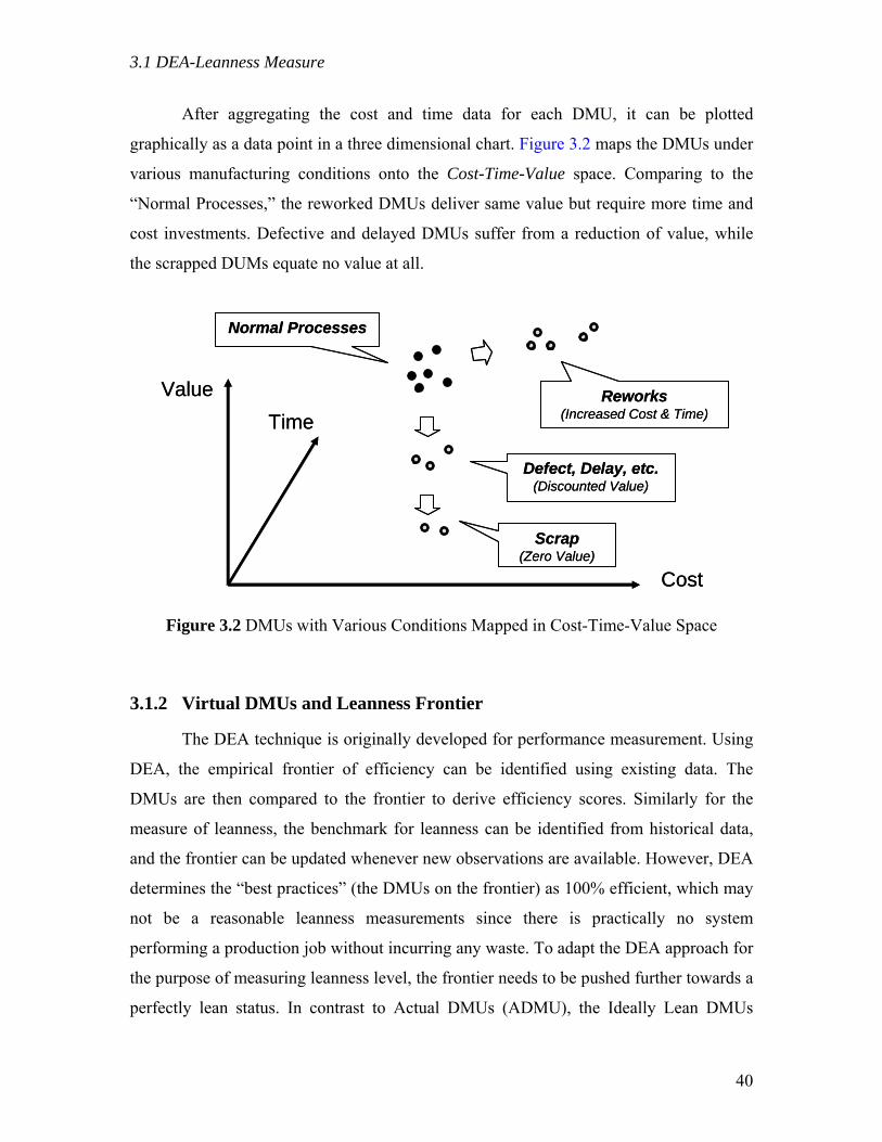
3.1 DEA-Leanness Measure
After aggregating the cost and time data for each DMU, it can be plotted
graphically as a data point in a three dimensional chart. Figure 3.2 maps the DMUs under
various manufacturing conditions onto the Cost-Time-Value space. Comparing to the
“Normal Processes,” the reworked DMUs deliver same value but require more time and
cost investments. Defective and delayed DMUs suffer from a reduction of value, while
the scrapped DUMs equate no value at all.
Cost
TimeValue
Normal Processes
Defect, Delay, etc.(Discounted Value)
Scrap(Zero Value)
Reworks(Increased Cost & Time)
Cost
TimeValue
Normal Processes
Defect, Delay, etc.(Discounted Value)
Scrap(Zero Value)
Reworks(Increased Cost & Time)
Figure 3.2 DMUs with Various Conditions Mapped in Cost-Time-Value Space
3.1.2 Virtual DMUs and Leanness Frontier
The DEA technique is originally developed for performance measurement. Using
DEA, the empirical frontier of efficiency can be identified using existing data. The
DMUs are then compared to the frontier to derive efficiency scores. Similarly for the
measure of leanness, the benchmark for leanness can be identified from historical data,
and the frontier can be updated whenever new observations are available. However, DEA
determines the “best practices” (the DMUs on the frontier) as 100% efficient, which may
not be a reasonable leanness measurements since there is practically no system
performing a production job without incurring any waste. To adapt the DEA approach for
the purpose of measuring leanness level, the frontier needs to be pushed further towards a
perfectly lean status. In contrast to Actual DMUs (ADMU), the Ideally Lean DMUs
40

3.1 DEA-Leanness Measure
(IDMU) are created virtually in order to push the frontier toward ideal leanness. Figure
3.3 demonstrates this concept by showing the DMUs and different levels of frontiers on a
Cost-Time diagram where the DMUs are normalized into same output Value.
Time
Cost
(100%) ?
(100%)
ActualDMUs
Ideal DMUs
RemoveNon-Value-AddedCost & Time
Time
Cost
(100%) ?
(100%)
ActualDMUsActualDMUs
Ideal DMUsIdeal DMUs
RemoveNon-Value-AddedCost & Time
Figure 3.3 Pushing Frontier towards Ideal Leanness by Ideal DMUs
To achieve a reasonable benchmark for leanness, the DEA-Leanness measure
pushes the frontier with the IDMUs which represent the perfect condition of the
production flow in the same value stream without any waste. That is to consider the
Value-Added (VA) inputs only. The input/output variables of the actual and ideally lean
DMUs are compared in Table 3.1.
Table 3.1 Actual DMU (ADMU) vs. Ideally Lean DMU (IDMU)
Actual DMU (ADMU) Ideally Lean DMU (IDMU)
Input Variables Total Cost
Total Time
Value-added (VA) Cost
Value-added (VA) Time
Output Variable Output Value Output Value
41
3.1 DEA-Leanness Measure
One of the characteristics of leanness measure is that the benchmark needs to be
updated over time. When the technologies of production or management skills improve
dramatically, new IDMUs need to push the leanness frontier further to update the
benchmark continuously. Therefore, if a frontier is obtained from only one data set, it is
possible that the frontier is not close enough to the ideal leanness due to some problems
associated with the data set. In order to ensure that the IDMUs are capable of achieving
an appropriate benchmark, the following three methods of obtaining IDMUs should be
considered.
Methods to Obtain IDMUs:
1) Virtually created by removing Non-Value-Added (NVA) inputs from the Actual
DMUs.
2) Obtained from the frontier of previous DEA-Leanness measurements of the same
system.
3) External benchmark obtained from other industrial group, consultants, etc.
Mathematical models have been developed for DEA which identify the Empirical
Frontier based on ADMUs. The IDMUs obtained from all sources push the frontier
toward the origin to become an adequate benchmark for leanness measurement. Figure
3.4 depicts the relationships between the ADMUs, IDMUs, wastes, and different levels of
frontiers on the Cost-Time diagram where Value has been normalized into same level.
From the ADMUs to the Empirical Frontier, individual operational inefficiencies are
identified, and the best practices (most efficient DMUs) form the frontier which is not
really lean. From the Empirical Frontier to the DEA-Leanness Frontier, wastes that can
be identified are removed from each DMU. If all wastes are identified and completely
removed, the Ultimate Leanness Frontier can be reached by the IDMUs. However, for
the production activities in reality, some types of wastes are easier to identify (e.g.,
waiting or defects), and some other types of wastes may not be easily recognized (e.g.,
over processing). Since it is difficult to identify all wastes, the ultimate leanness may not
be reached by the DEA-Leanness Frontier. A delicate analysis of value-added versus
non-value-added activities or a good source of external benchmarks can bring the two
42

3.1 DEA-Leanness Measure
frontiers closer. The Cost-Time-Value Analysis for building the DMUs is introduced in
the next section.
Cost
TimeADMUs
IDMUs
DEA-Leanness FrontierUltimate Leanness Frontier
Identifiable Wastes
Unidentifiable Wastes
Empirical Frontier
Cost
TimeADMUs
IDMUs
DEA-Leanness FrontierUltimate Leanness Frontier
Identifiable Wastes
Unidentifiable Wastes
Empirical Frontier
Figure 3.4 Pushing from the Empirical Frontier to the Ultimate Leanness
3.1.3 Cost-Time-Value Analysis
A Cost-Time-Value Analysis is developed to create ADMUs and IDMUs from
production data. In Figure 3.5, an example of a two-station manufacturing system with
three buffer areas is employed to demonstrate the procedure of the analysis. The
production processes of each work piece flowing through the system are mapped in the
Cost-Time diagram. The diagram differentiates value-added (VA) and non-value-added
(NVA) time spans according to the characteristics of the activities. Costs of each time
span are identified and differentiated into VA and NVA costs. The ADMUs and IDMUs
are then created using the cost, time and value data collected from this analysis. The
detailed procedure of the analysis is listed following the figure.
43

3.1 DEA-Leanness Measure
Cost
Time
OP1 OP2
NVATime 1
NVATime 2
NVATime 3
VATime 1
VATime 2
OP1 OP2
NVA Time
VA Time
IdealDMU
VA CostVA Time
Value
IdealIdealDMUDMU
VA CostVA Time
Value
ActualDMU
Total CostTotal Time
Value
ActualActualDMUDMU
Total CostTotal Time
Value
Output Value= Retail Price x Customer Satisfaction
VA Cost
NVA Cost
VA CostVA Cost
NVA CostNVA Cost
Figure 3.5 Cost-Time-Value Analysis for Creation of ADMUs and IDMUs
Cost-Time-Value Analysis for DMUs
Step 1: Identify the scope to be analyzed. In manufacturing systems, the scope can be
a cell, a production line, a department, or the whole shop floor, depending on
the scope that the Value Stream Map covers.
Step 2: Map the value stream. Identify the customer, supplier, workstations
(operations), online buffer areas, and offline inventory that are involved in the
selected scope of value stream.
Step 3: Collect cost and time data. For each work piece that flows through the value
stream, record the time and other resources (labor, machine, material, etc.) that
are consumed by each production activities.
Step 4: Identify VA and NVA activities. Based on the customer defined value and the
seven types of wastes in Toyota Production System, differentiate the VA
activities from the NVA activities.
Step 5: Separate VA time and NVA time. For each work piece, identify the VA and
NVA time spans over the total manufacturing lead time.
Step 6: Identify VA and NVA costs for each time span. The resources consumed by
each process are translated into costs. During VA time spans, VA costs and
44
3.1 DEA-Leanness Measure
NVA costs may exist simultaneously. NVA time spans contain only NVA costs.
The two categories of costs are plotted as line segments in the Cost-Time
diagram. The final heights represent the accumulated VA and NVA costs.
Step 7: Summarize total costs, total time, and created value to generate ADMUs.
An ADMU is an observation of the actual production of a single work piece.
The actual time and costs invested on the work piece are the input variables for
the ADMU. The created value is the only output variable.
Step 8: Summarize the VA cost and VA time to create IDMUs. An IDMU is
obtained from each ADMU by removing NVA costs and NVA time spans from
the corresponding ADMU. Therefore, only the VA costs and VA time spans are
included in IDMUs.
Step 9: Run DEAL model with the created ADMUs and IDMUs. The two types of
DMUs are used in the DEA-Leanness measurement to evaluate the leanness
level of the production of each work piece.
For the Cost-Time-Value Analysis, a cost breakdown of each process is required
to identify VA and NVA costs. More details being included in the cost breakdown can
lead to more accurate evaluation of leanness. Figure 3.6 illustrates a procedure of the cost
breakdown for DEA-Leanness Measure. Identifying the costs associated with an
individual work piece is not always trivial since some types of cost are shared by a set of
work pieces. In order to allocate the costs to each work piece, identifying the aggregated
cost of the selected value stream over a period would be a more feasible starting point.
The aggregated costs, including material costs and conversion costs, can then be
differentiated into Time-based Costs and Unit-based Costs for each work piece. The final
values of the cost variable for the DEA-Leanness Measure are obtained by further
differentiating the costs based on the VA and NVA time spans in the Cost-Time diagram
as shown in Figure 3.6.
After collecting all the required data, the DEA-Leanness Measure can be
performed using the mathematical models developed by previous researchers. Two
different models are employed in this research which are introduced in the following
sections.
45
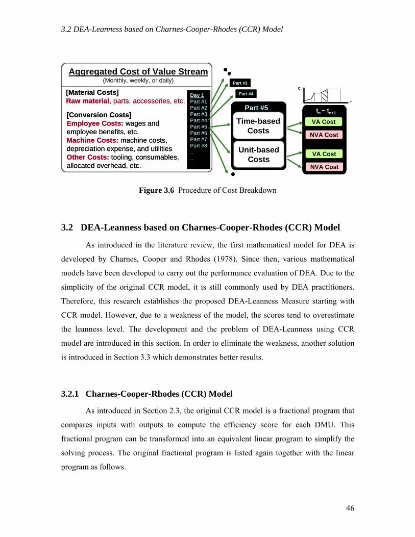
3.2 DEA-Leanness based on Charnes-Cooper-Rhodes (CCR) Model
Aggregated Cost of Value Stream(Monthly, weekly, or daily)
Unit-basedCosts
Day 1Part #1Part #2Part #3Part #4Part #5Part #6Part #7Part #8......
Part #5
Time-basedCosts
Part #3
Part #4
VA Cost
NVA Cost
VA Cost
NVA Cost
tn ~ tn+1
T
C[Material Costs]Raw material, parts, accessories, etc.
[Conversion Costs]Employee Costs: wages and employee benefits, etc.Machine Costs: machine costs, depreciation expense, and utilitiesOther Costs: tooling, consumables, allocated overhead, etc.
[Material Costs]Raw material, parts, accessories, etc.
[Conversion Costs]Employee Costs: wages and employee benefits, etc.Machine Costs: machine costs, depreciation expense, and utilitiesOther Costs: tooling, consumables, allocated overhead, etc.
Figure 3.6 Procedure of Cost Breakdown
3.2 DEA-Leanness based on Charnes-Cooper-Rhodes (CCR) Model
As introduced in the literature review, the first mathematical model for DEA is
developed by Charnes, Cooper and Rhodes (1978). Since then, various mathematical
models have been developed to carry out the performance evaluation of DEA. Due to the
simplicity of the original CCR model, it is still commonly used by DEA practitioners.
Therefore, this research establishes the proposed DEA-Leanness Measure starting with
CCR model. However, due to a weakness of the model, the scores tend to overestimate
the leanness level. The development and the problem of DEA-Leanness using CCR
model are introduced in this section. In order to eliminate the weakness, another solution
is introduced in Section 3.3 which demonstrates better results.
3.2.1 Charnes-Cooper-Rhodes (CCR) Model
As introduced in Section 2.3, the original CCR model is a fractional program that
compares inputs with outputs to compute the efficiency score for each DMU. This
fractional program can be transformed into an equivalent linear program to simplify the
solving process. The original fractional program is listed again together with the linear
program as follows.
46
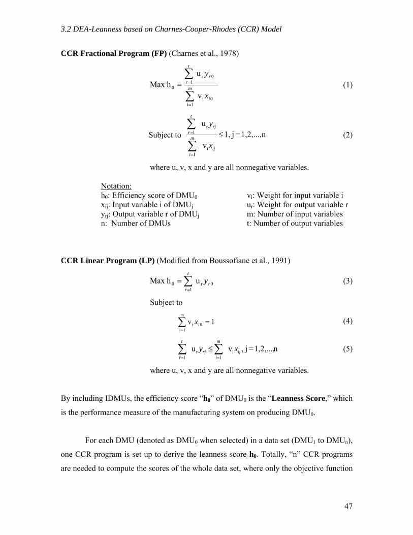
3.2 DEA-Leanness based on Charnes-Cooper-Rhodes (CCR) Model
CCR Fractional Program (FP) (Charnes et al., 1978)
∑
∑
=
== m
ii
t
rr
x
y
10i
10r
0
v
u hMax (1)
Subject to n1,2,...,=j1, v
u
i1
r1 ≤
∑
∑
=
=
ij
m
i
rj
t
r
x
y (2)
where u, v, x and y are all nonnegative variables.
Notation: h0: Efficiency score of DMU0xij: Input variable i of DMUjyrj: Output variable r of DMUj n: Number of DMUs
vi: Weight for input variable i ur: Weight for output variable r m: Number of input variables t: Number of output variables
CCR Linear Program (LP) (Modified from Boussofiane et al., 1991)
∑=
=t
rry
10r0 u hMax (3)
Subject to
(4) 1v1
0i =∑=
m
iix
n1,2,...,=j , vu i1
r1
ij
m
irj
t
rxy ∑∑
==
≤ (5)
where u, v, x and y are all nonnegative variables.
By including IDMUs, the efficiency score “h0” of DMU0 is the “Leanness Score,” which
is the performance measure of the manufacturing system on producing DMU0.
For each DMU (denoted as DMU0 when selected) in a data set (DMU1 to DMUn),
one CCR program is set up to derive the leanness score h0. Totally, “n” CCR programs
are needed to compute the scores of the whole data set, where only the objective function
47
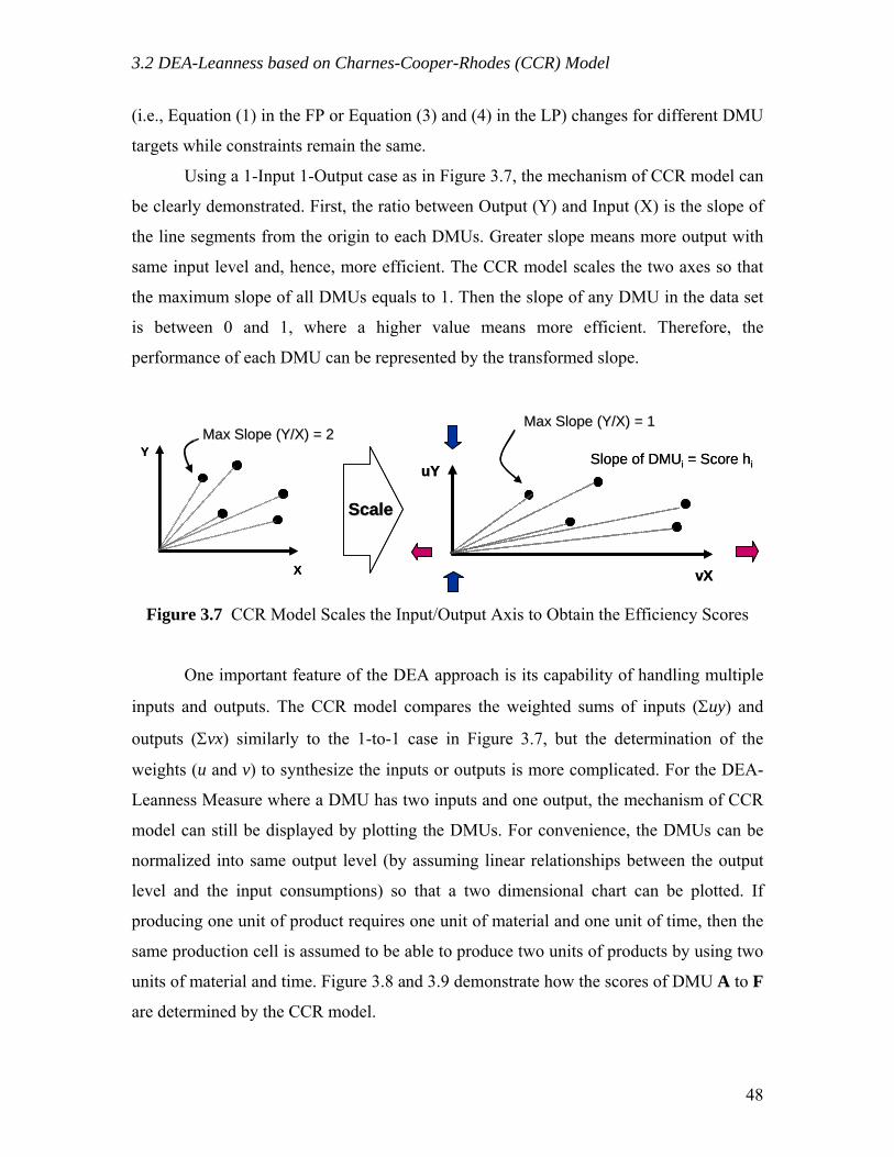
3.2 DEA-Leanness based on Charnes-Cooper-Rhodes (CCR) Model
(i.e., Equation (1) in the FP or Equation (3) and (4) in the LP) changes for different DMU
targets while constraints remain the same.
Using a 1-Input 1-Output case as in Figure 3.7, the mechanism of CCR model can
be clearly demonstrated. First, the ratio between Output (Y) and Input (X) is the slope of
the line segments from the origin to each DMUs. Greater slope means more output with
same input level and, hence, more efficient. The CCR model scales the two axes so that
the maximum slope of all DMUs equals to 1. Then the slope of any DMU in the data set
is between 0 and 1, where a higher value means more efficient. Therefore, the
performance of each DMU can be represented by the transformed slope.
X
YMax Slope (Y/X) = 2Max Slope (Y/X) = 2
vX
uY
Max Slope (Y/X) = 1Max Slope (Y/X) = 1
Slope of DMUi = Score hi
ScaleScale
X
YMax Slope (Y/X) = 2Max Slope (Y/X) = 2
vX
uY
Max Slope (Y/X) = 1Max Slope (Y/X) = 1
Slope of DMUi = Score hi
ScaleScale
Figure 3.7 CCR Model Scales the Input/Output Axis to Obtain the Efficiency Scores
One important feature of the DEA approach is its capability of handling multiple
inputs and outputs. The CCR model compares the weighted sums of inputs (Σuy) and
outputs (Σvx) similarly to the 1-to-1 case in Figure 3.7, but the determination of the
weights (u and v) to synthesize the inputs or outputs is more complicated. For the DEA-
Leanness Measure where a DMU has two inputs and one output, the mechanism of CCR
model can still be displayed by plotting the DMUs. For convenience, the DMUs can be
normalized into same output level (by assuming linear relationships between the output
level and the input consumptions) so that a two dimensional chart can be plotted. If
producing one unit of product requires one unit of material and one unit of time, then the
same production cell is assumed to be able to produce two units of products by using two
units of material and time. Figure 3.8 and 3.9 demonstrate how the scores of DMU A to F
are determined by the CCR model.
48
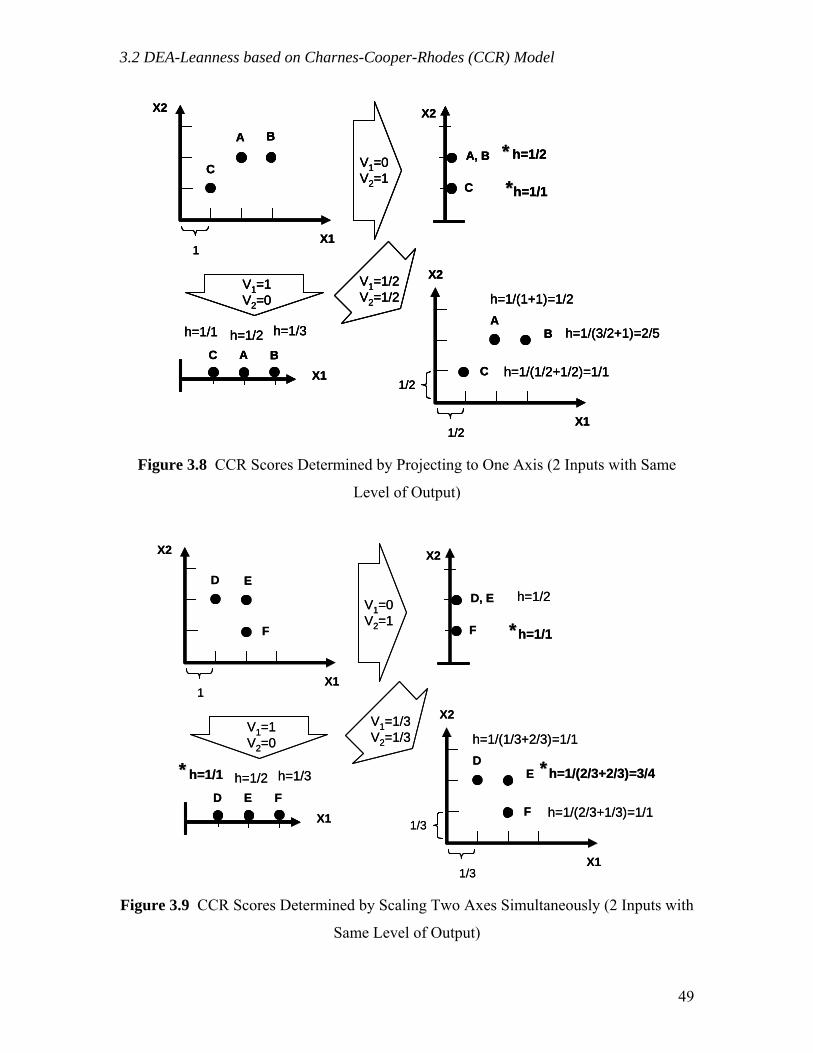
3.2 DEA-Leanness based on Charnes-Cooper-Rhodes (CCR) Model
1
A B
CA, B
C
X1
X2
h=1/2
h=1/1
A BC
h=1/1 h=1/2 h=1/3
V1=0V2=1
V1=1V2=0
X1
X2
**
**
V1=1/2V2=1/2
1/2
B
C
A
X1
X2
h=1/(1/2+1/2)=1/1
h=1/(1+1)=1/2
1/2
h=1/(3/2+1)=2/5
1
A B
CA, B
C
X1
X2
h=1/2
h=1/1
A BC
h=1/1 h=1/2 h=1/3
V1=0V2=1
V1=1V2=0
X1
X2
**
**
1
A B
CA, B
C
X1
X2
h=1/2
h=1/1
A BC
h=1/1 h=1/2 h=1/3
V1=0V2=1
V1=1V2=0
X1
X2
**
**
V1=1/2V2=1/2
1/2
B
C
A
X1
X2
h=1/(1/2+1/2)=1/1
h=1/(1+1)=1/2
1/2
h=1/(3/2+1)=2/5
V1=1/2V2=1/2
1/2
B
C
A
X1
X2
h=1/(1/2+1/2)=1/1
h=1/(1+1)=1/2
1/2
h=1/(3/2+1)=2/5
Figure 3.8 CCR Scores Determined by Projecting to One Axis (2 Inputs with Same
Level of Output)
1
E
F
DD, E
F
X1
X2
h=1/2
h=1/1
E FD
h=1/1 h=1/2 h=1/3
V1=0V2=1
V1=1V2=0
X1
X2
V1=1/3V2=1/3
1/3
E
F
D
X1
X2
h=1/(2/3+1/3)=1/1
h=1/(2/3+2/3)=3/4
h=1/(1/3+2/3)=1/1
**
**
**
1/3
1
E
F
DD, E
F
X1
X2
h=1/2
h=1/1
E FD
h=1/1 h=1/2 h=1/3
V1=0V2=1
V1=1V2=0
X1
X2
V1=1/3V2=1/3
1/3
E
F
D
X1
X2
h=1/(2/3+1/3)=1/1
h=1/(2/3+2/3)=3/4
h=1/(1/3+2/3)=1/1
**
**
**
1/3
Figure 3.9 CCR Scores Determined by Scaling Two Axes Simultaneously (2 Inputs with
Same Level of Output)
49
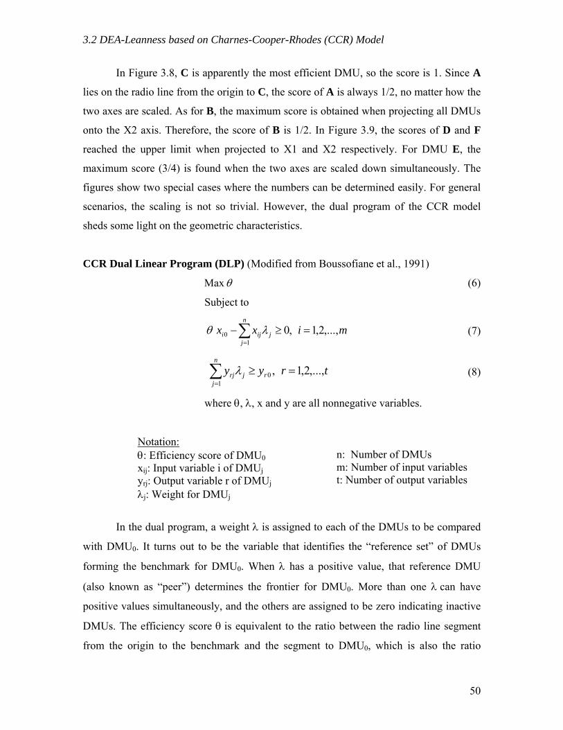
3.2 DEA-Leanness based on Charnes-Cooper-Rhodes (CCR) Model
In Figure 3.8, C is apparently the most efficient DMU, so the score is 1. Since A
lies on the radio line from the origin to C, the score of A is always 1/2, no matter how the
two axes are scaled. As for B, the maximum score is obtained when projecting all DMUs
onto the X2 axis. Therefore, the score of B is 1/2. In Figure 3.9, the scores of D and F
reached the upper limit when projected to X1 and X2 respectively. For DMU E, the
maximum score (3/4) is found when the two axes are scaled down simultaneously. The
figures show two special cases where the numbers can be determined easily. For general
scenarios, the scaling is not so trivial. However, the dual program of the CCR model
sheds some light on the geometric characteristics.
CCR Dual Linear Program (DLP) (Modified from Boussofiane et al., 1991)
θMax (6)
Subject to
mixx j
n
jiji ,...,2,1,0
10 =≥−∑
=
λθ (7)
tryy rj
n
jrj ,...,2,1,0
1=≥∑
=
λ (8)
where θ, λ, x and y are all nonnegative variables.
Notation: θ: Efficiency score of DMU0xij: Input variable i of DMUjyrj: Output variable r of DMUj
λj: Weight for DMUj
n: Number of DMUs m: Number of input variables t: Number of output variables
In the dual program, a weight λ is assigned to each of the DMUs to be compared
with DMU0. It turns out to be the variable that identifies the “reference set” of DMUs
forming the benchmark for DMU0. When λ has a positive value, that reference DMU
(also known as “peer”) determines the frontier for DMU0. More than one λ can have
positive values simultaneously, and the others are assigned to be zero indicating inactive
DMUs. The efficiency score θ is equivalent to the ratio between the radio line segment
from the origin to the benchmark and the segment to DMU0, which is also the ratio
50

3.2 DEA-Leanness based on Charnes-Cooper-Rhodes (CCR) Model
between “efficient segment” and “efficient + inefficient segments.” The “reference set”
contains the DMUs that form the section of frontier where the intersection occurs.
Actually, the λ’s sum up to 1, which makes the benchmark of DMU0 a convex
combination of the reference set. Figure 3.10 illustrates the relationships between DMU,
reference set and the score.
(100%)
(100%)
(100%)
(55%)
(55%)
FrontierFrontier
A
BF
X1
E
CD
X2 (35%)G
Inefficient
Inefficient
Efficient
E’F’
O
(100%)
Figure 3.10 Leanness Scores Obtained from CCR Model
In the figure, A, B, C and D are the most efficient DMUs which forms the frontier.
They are also their own reference set, which makes the scoring ratio 100%. E’ and F’ are
the intersections (also known as “projection point”) of the frontier and the radio lines.
They are the benchmarks for E and F to calculate the scoring ratio. As shown in the
figure, E’ is a convex combination of C and D. Therefore, C and D are the two DMUs in
the reference set of E. As for F, the projection point F’ lies on the horizontal section.
Therefore, DMU D is the sole reference for F because the other end of the frontier goes
to infinity. DMU G lies on the radio line from O through C, so C is also the sole
reference for G. These relationships are summarized in Table 3.2.
For DEA-Leanness Measure, the two inputs are Time and Cost, and the output is
Value. Using the expression similar to Figure 3.10, the leanness score is the ratio between
the “Value-added Investments” and the “Value-added + Non-value-added Investments.”
It is an indication of how far away the DMU is from the ideally lean status. Using the
51
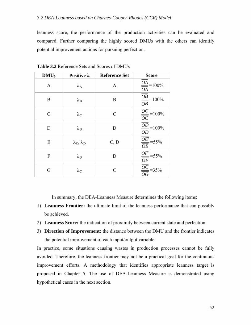
3.2 DEA-Leanness based on Charnes-Cooper-Rhodes (CCR) Model
leanness score, the performance of the production activities can be evaluated and
compared. Further comparing the highly scored DMUs with the others can identify
potential improvement actions for pursuing perfection.
Table 3.2 Reference Sets and Scores of DMUs
DMU0 Positive λ Reference Set Score
A λA A OAOA =100%
B λB B BOBO =100%
C λC C OC
CO =100%
D λD D OD
DO =100%
E λC, λD C, D OE
EO ' =55%
F λD D OF
FO ' =55%
G λC C OG
CO =35%
In summary, the DEA-Leanness Measure determines the following items:
1) Leanness Frontier: the ultimate limit of the leanness performance that can possibly
be achieved.
2) Leanness Score: the indication of proximity between current state and perfection.
3) Direction of Improvement: the distance between the DMU and the frontier indicates
the potential improvement of each input/output variable.
In practice, some situations causing wastes in production processes cannot be fully
avoided. Therefore, the leanness frontier may not be a practical goal for the continuous
improvement efforts. A methodology that identifies appropriate leanness target is
proposed in Chapter 5. The use of DEA-Leanness Measure is demonstrated using
hypothetical cases in the next section.
52

3.2 DEA-Leanness based on Charnes-Cooper-Rhodes (CCR) Model
3.2.2 Hypothetical Cases Using CCR Model
In this section, hypothetical cases are created to test the DEA-Leanness Measure
based on CCR model. The basic setting of the cases is a dedicated flow line with three
workstations as shown in Figure 3.11. The production line produces one type of product.
There is no buffer between workstations, so the operators need to wait after finishing a
product when the next station is busy. Also, the downstream operators need to wait for
the previous station to provide the required material. The detailed settings are listed after
Figure 3.11. Table 3.3 lists the detailed cost breakdown.
WS1(OP1)
WS2(OP2)
WS3(OP3)
Figure 3.11 Hypothetical Case: Dedicated Flow Line with Three Workstations
Hypothetical Case Basic Settings:
Production Schedule: 20 units of Product A
Available Time: 8 hours/day
Takt Time: 24 minutes/unit
Output: Value = 1 if not delayed or defective, otherwise Value < 1
Processing Time: (Data generated by MS Excel Random Number Generator) OP1: 20 min. ± 2 min. (Uniformly distributed, random seed: #1000)
OP2: 20 min. ± 2 min. (Uniformly distributed, random seed: #2000) OP3: 20 min. ± 2 min. (Uniformly distributed, random seed: #3000)
Table 3.3 Costs Breakdown in Case 1
WS1 WS2 WS3 VA NVA VA NVA VA NVA
Labor $0.1/min 0 $0.1/min 0 $0.1/min 0 Machine $0.2/min 0 $0.2/min 0 $0.25/min 0 Material $20/unit $1/unit $3/unit $0.5/unit $2/unit 0 Miscellaneous (Energy, Space, etc.) $0.01/min $0.01/min $0.01/min $0.01/min $0.01/min $0.01/min
53
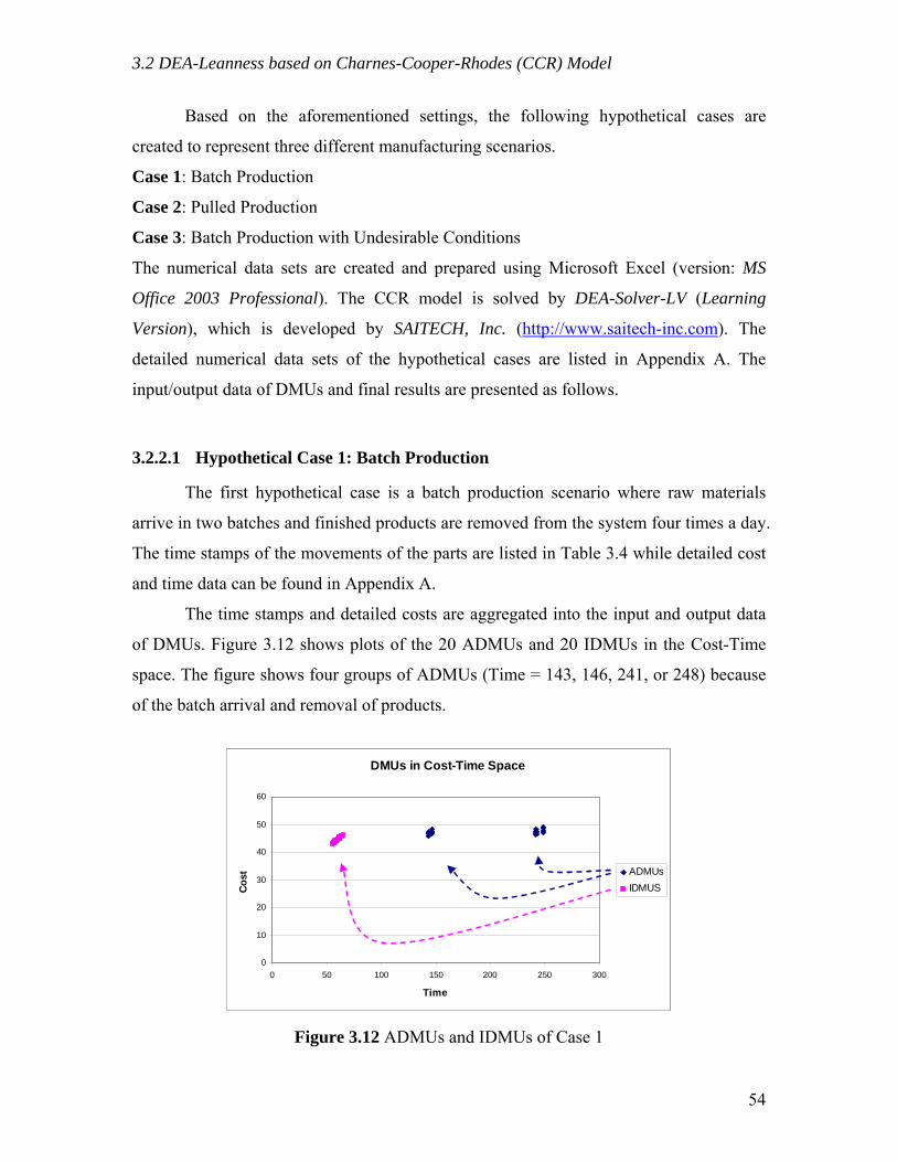
3.2 DEA-Leanness based on Charnes-Cooper-Rhodes (CCR) Model
Based on the aforementioned settings, the following hypothetical cases are
created to represent three different manufacturing scenarios.
Case 1: Batch Production
Case 2: Pulled Production
Case 3: Batch Production with Undesirable Conditions
The numerical data sets are created and prepared using Microsoft Excel (version: MS
Office 2003 Professional). The CCR model is solved by DEA-Solver-LV (Learning
Version), which is developed by SAITECH, Inc. (http://www.saitech-inc.com). The
detailed numerical data sets of the hypothetical cases are listed in Appendix A. The
input/output data of DMUs and final results are presented as follows.
3.2.2.1 Hypothetical Case 1: Batch Production
The first hypothetical case is a batch production scenario where raw materials
arrive in two batches and finished products are removed from the system four times a day.
The time stamps of the movements of the parts are listed in Table 3.4 while detailed cost
and time data can be found in Appendix A.
The time stamps and detailed costs are aggregated into the input and output data
of DMUs. Figure 3.12 shows plots of the 20 ADMUs and 20 IDMUs in the Cost-Time
space. The figure shows four groups of ADMUs (Time = 143, 146, 241, or 248) because
of the batch arrival and removal of products.
DMUs in Cost-Time Space
0
10
20
30
40
50
60
0 50 100 150 200 250 300
Time
Cost
ADMUsIDMUS
DMUs in Cost-Time Space
0
10
20
30
40
50
60
0 50 100 150 200 250 300
Time
Cost
ADMUsIDMUS
Figure 3.12 ADMUs and IDMUs of Case 1
54
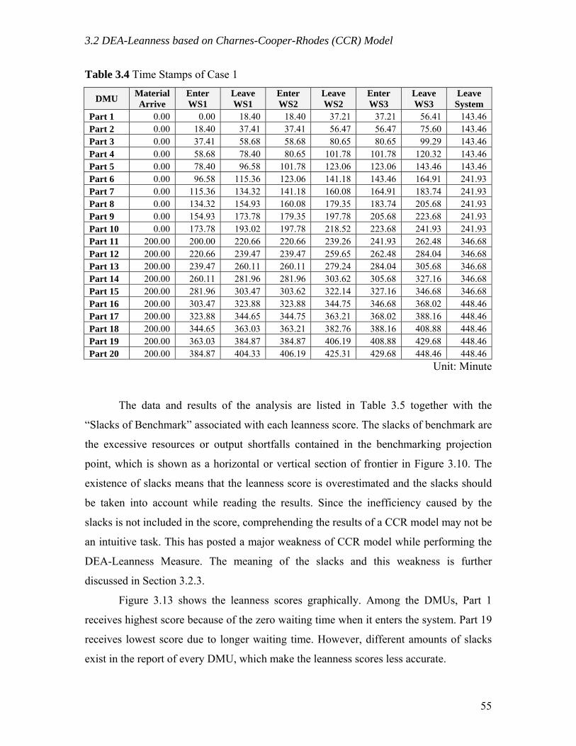
3.2 DEA-Leanness based on Charnes-Cooper-Rhodes (CCR) Model
Table 3.4 Time Stamps of Case 1
DMU Material Arrive
Enter WS1
Leave WS1
Enter WS2
Leave WS2
Enter WS3
Leave WS3
Leave System
Part 1 0.00 0.00 18.40 18.40 37.21 37.21 56.41 143.46 Part 2 0.00 18.40 37.41 37.41 56.47 56.47 75.60 143.46 Part 3 0.00 37.41 58.68 58.68 80.65 80.65 99.29 143.46 Part 4 0.00 58.68 78.40 80.65 101.78 101.78 120.32 143.46 Part 5 0.00 78.40 96.58 101.78 123.06 123.06 143.46 143.46 Part 6 0.00 96.58 115.36 123.06 141.18 143.46 164.91 241.93 Part 7 0.00 115.36 134.32 141.18 160.08 164.91 183.74 241.93 Part 8 0.00 134.32 154.93 160.08 179.35 183.74 205.68 241.93 Part 9 0.00 154.93 173.78 179.35 197.78 205.68 223.68 241.93 Part 10 0.00 173.78 193.02 197.78 218.52 223.68 241.93 241.93 Part 11 200.00 200.00 220.66 220.66 239.26 241.93 262.48 346.68 Part 12 200.00 220.66 239.47 239.47 259.65 262.48 284.04 346.68 Part 13 200.00 239.47 260.11 260.11 279.24 284.04 305.68 346.68 Part 14 200.00 260.11 281.96 281.96 303.62 305.68 327.16 346.68 Part 15 200.00 281.96 303.47 303.62 322.14 327.16 346.68 346.68 Part 16 200.00 303.47 323.88 323.88 344.75 346.68 368.02 448.46 Part 17 200.00 323.88 344.65 344.75 363.21 368.02 388.16 448.46 Part 18 200.00 344.65 363.03 363.21 382.76 388.16 408.88 448.46 Part 19 200.00 363.03 384.87 384.87 406.19 408.88 429.68 448.46 Part 20 200.00 384.87 404.33 406.19 425.31 429.68 448.46 448.46
Unit: Minute
The data and results of the analysis are listed in Table 3.5 together with the
“Slacks of Benchmark” associated with each leanness score. The slacks of benchmark are
the excessive resources or output shortfalls contained in the benchmarking projection
point, which is shown as a horizontal or vertical section of frontier in Figure 3.10. The
existence of slacks means that the leanness score is overestimated and the slacks should
be taken into account while reading the results. Since the inefficiency caused by the
slacks is not included in the score, comprehending the results of a CCR model may not be
an intuitive task. This has posted a major weakness of CCR model while performing the
DEA-Leanness Measure. The meaning of the slacks and this weakness is further
discussed in Section 3.2.3.
Figure 3.13 shows the leanness scores graphically. Among the DMUs, Part 1
receives highest score because of the zero waiting time when it enters the system. Part 19
receives lowest score due to longer waiting time. However, different amounts of slacks
exist in the report of every DMU, which make the leanness scores less accurate.
55

3.2 DEA-Leanness based on Charnes-Cooper-Rhodes (CCR) Model
Table 3.5 Data and Results of Case 1 Using CCR Model
Inputs Output Score Slacks of Benchmark DMU Total
Time VA
Time Total Cost
VA Cost Value Leanness
Score Time
(Excess) Cost
(Excess) Value
(Shortfall) Part 1 143.46 56.41 45.82 43.45 1 0.94 79.47 0 0 Part 2 143.46 57.19 46.05 43.69 1 0.93 78.79 0 0 Part 3 143.46 61.89 47.43 45.12 1 0.91 74.88 0 0 Part 4 143.46 59.39 46.68 44.34 1 0.92 76.98 0 0 Part 5 143.46 59.86 46.91 44.58 1 0.92 76.32 0 0 Part 6 241.93 58.34 47.49 44.16 1 0.91 163.94 0 0 Part 7 241.93 56.69 46.87 43.52 1 0.92 166.87 0 0 Part 8 241.93 61.82 48.56 45.26 1 0.89 159.12 0 0 Part 9 241.93 55.28 46.40 43.04 1 0.93 169.10 0 0 Part 10 241.93 58.23 47.30 43.96 1 0.91 164.84 0 0 Part 11 146.68 59.81 46.94 44.57 1 0.92 79.21 0 0 Part 12 146.68 60.55 47.21 44.85 1 0.91 78.43 0 0 Part 13 146.68 61.42 47.47 45.12 1 0.91 77.69 0 0 Part 14 146.68 64.99 48.54 46.22 1 0.89 74.77 0 0 Part 15 146.68 59.55 46.81 44.44 1 0.92 79.59 0 0 Part 16 248.46 62.63 48.84 45.48 1 0.88 163.66 0 0 Part 17 248.46 59.36 47.80 44.41 1 0.90 168.42 0 0 Part 18 248.46 58.66 47.62 44.22 1 0.90 169.27 0 0 Part 19 248.46 63.96 49.21 45.87 1 0.87 162.01 0 0 Part 20 248.46 57.36 47.13 43.72 1 0.91 171.59 0 0
DEA-Leanness Score (CCR Model): Case 1
0
0.1
0.20.3
0.4
0.5
0.6
0.70.8
0.9
1
1 2 3 4 5 6 7 8 9 10 11 12 13 14 15 16 17 18 19 20
DMU
Lean
nes
ADMUIDMU
Figure 3.13 Leanness Scores of Case 1 Using CCR Model
56
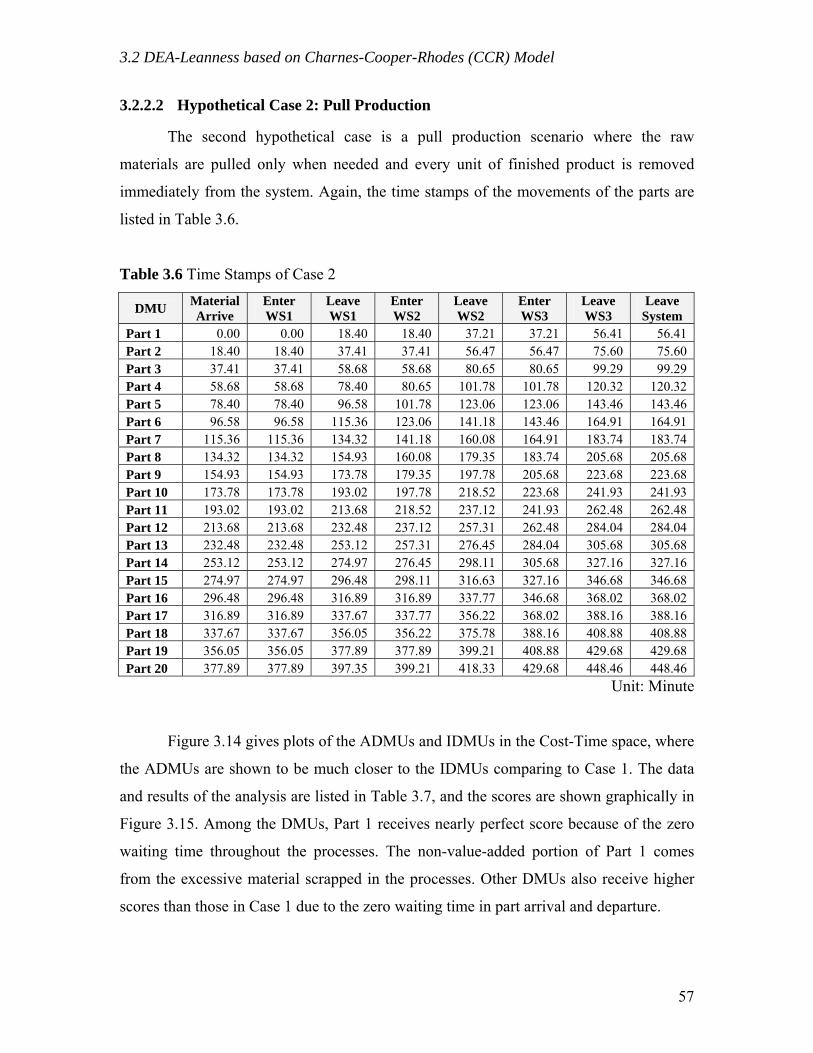
3.2 DEA-Leanness based on Charnes-Cooper-Rhodes (CCR) Model
3.2.2.2 Hypothetical Case 2: Pull Production
The second hypothetical case is a pull production scenario where the raw
materials are pulled only when needed and every unit of finished product is removed
immediately from the system. Again, the time stamps of the movements of the parts are
listed in Table 3.6.
Table 3.6 Time Stamps of Case 2
DMU Material Arrive
Enter WS1
Leave WS1
Enter WS2
Leave WS2
Enter WS3
Leave WS3
Leave System
Part 1 0.00 0.00 18.40 18.40 37.21 37.21 56.41 56.41 Part 2 18.40 18.40 37.41 37.41 56.47 56.47 75.60 75.60 Part 3 37.41 37.41 58.68 58.68 80.65 80.65 99.29 99.29 Part 4 58.68 58.68 78.40 80.65 101.78 101.78 120.32 120.32 Part 5 78.40 78.40 96.58 101.78 123.06 123.06 143.46 143.46 Part 6 96.58 96.58 115.36 123.06 141.18 143.46 164.91 164.91 Part 7 115.36 115.36 134.32 141.18 160.08 164.91 183.74 183.74 Part 8 134.32 134.32 154.93 160.08 179.35 183.74 205.68 205.68 Part 9 154.93 154.93 173.78 179.35 197.78 205.68 223.68 223.68 Part 10 173.78 173.78 193.02 197.78 218.52 223.68 241.93 241.93 Part 11 193.02 193.02 213.68 218.52 237.12 241.93 262.48 262.48 Part 12 213.68 213.68 232.48 237.12 257.31 262.48 284.04 284.04 Part 13 232.48 232.48 253.12 257.31 276.45 284.04 305.68 305.68 Part 14 253.12 253.12 274.97 276.45 298.11 305.68 327.16 327.16 Part 15 274.97 274.97 296.48 298.11 316.63 327.16 346.68 346.68 Part 16 296.48 296.48 316.89 316.89 337.77 346.68 368.02 368.02 Part 17 316.89 316.89 337.67 337.77 356.22 368.02 388.16 388.16 Part 18 337.67 337.67 356.05 356.22 375.78 388.16 408.88 408.88 Part 19 356.05 356.05 377.89 377.89 399.21 408.88 429.68 429.68 Part 20 377.89 377.89 397.35 399.21 418.33 429.68 448.46 448.46
Unit: Minute
Figure 3.14 gives plots of the ADMUs and IDMUs in the Cost-Time space, where
the ADMUs are shown to be much closer to the IDMUs comparing to Case 1. The data
and results of the analysis are listed in Table 3.7, and the scores are shown graphically in
Figure 3.15. Among the DMUs, Part 1 receives nearly perfect score because of the zero
waiting time throughout the processes. The non-value-added portion of Part 1 comes
from the excessive material scrapped in the processes. Other DMUs also receive higher
scores than those in Case 1 due to the zero waiting time in part arrival and departure.
57
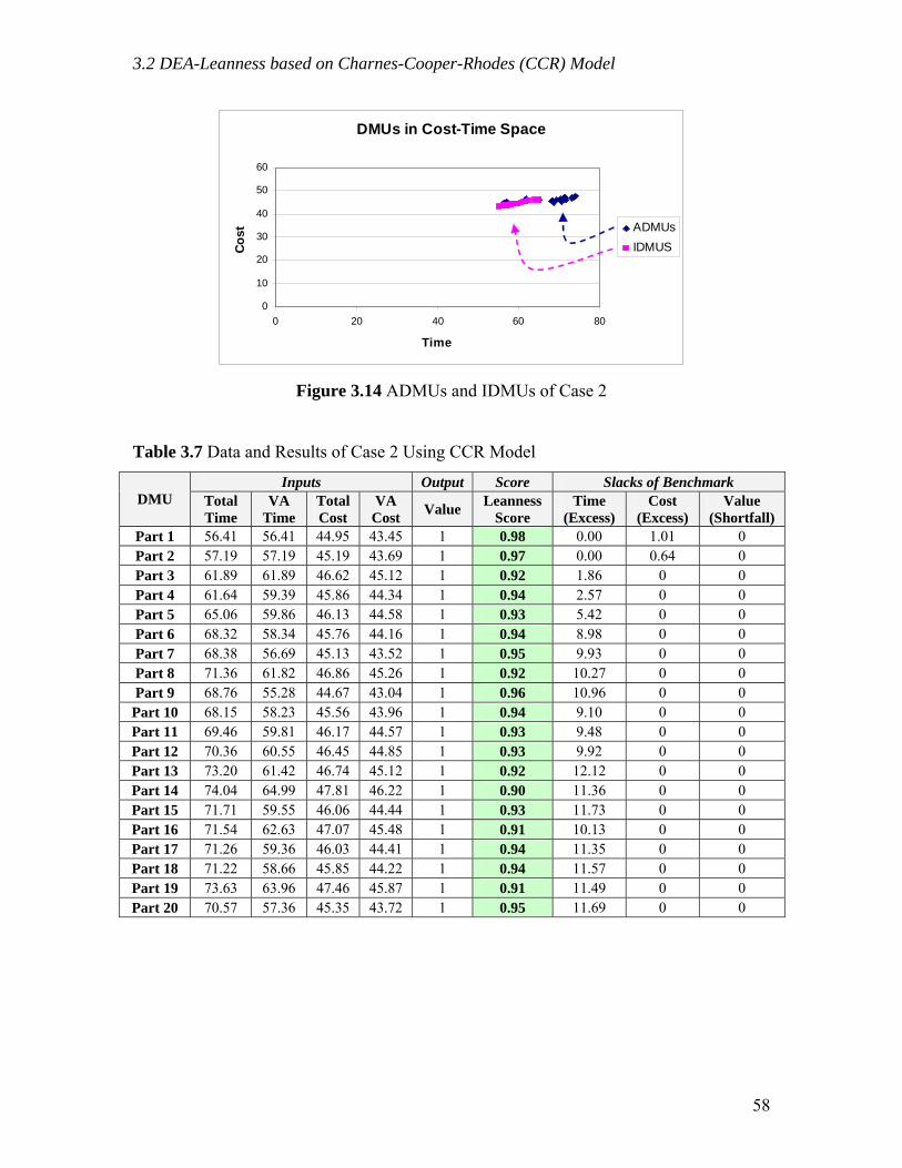
3.2 DEA-Leanness based on Charnes-Cooper-Rhodes (CCR) Model
DMUs in Cost-Time Space
0
10
20
30
40
50
60
0 20 40 60 80
Time
Cost
ADMUsIDMUS
Figure 3.14 ADMUs and IDMUs of Case 2
Table 3.7 Data and Results of Case 2 Using CCR Model
Inputs Output Score Slacks of Benchmark DMU Total
Time VA
Time Total Cost
VA Cost Value Leanness
Score Time
(Excess) Cost
(Excess) Value
(Shortfall) Part 1 56.41 56.41 44.95 43.45 1 0.98 0.00 1.01 0 Part 2 57.19 57.19 45.19 43.69 1 0.97 0.00 0.64 0 Part 3 61.89 61.89 46.62 45.12 1 0.92 1.86 0 0 Part 4 61.64 59.39 45.86 44.34 1 0.94 2.57 0 0 Part 5 65.06 59.86 46.13 44.58 1 0.93 5.42 0 0 Part 6 68.32 58.34 45.76 44.16 1 0.94 8.98 0 0 Part 7 68.38 56.69 45.13 43.52 1 0.95 9.93 0 0 Part 8 71.36 61.82 46.86 45.26 1 0.92 10.27 0 0 Part 9 68.76 55.28 44.67 43.04 1 0.96 10.96 0 0 Part 10 68.15 58.23 45.56 43.96 1 0.94 9.10 0 0 Part 11 69.46 59.81 46.17 44.57 1 0.93 9.48 0 0 Part 12 70.36 60.55 46.45 44.85 1 0.93 9.92 0 0 Part 13 73.20 61.42 46.74 45.12 1 0.92 12.12 0 0 Part 14 74.04 64.99 47.81 46.22 1 0.90 11.36 0 0 Part 15 71.71 59.55 46.06 44.44 1 0.93 11.73 0 0 Part 16 71.54 62.63 47.07 45.48 1 0.91 10.13 0 0 Part 17 71.26 59.36 46.03 44.41 1 0.94 11.35 0 0 Part 18 71.22 58.66 45.85 44.22 1 0.94 11.57 0 0 Part 19 73.63 63.96 47.46 45.87 1 0.91 11.49 0 0 Part 20 70.57 57.36 45.35 43.72 1 0.95 11.69 0 0
58

3.2 DEA-Leanness based on Charnes-Cooper-Rhodes (CCR) Model
DEA-Leanness Score (CCR Model): Case 2
0
0.10.2
0.3
0.4
0.50.6
0.7
0.80.9
1
1 2 3 4 5 6 7 8 9 10 11 12 13 14 15 16 17 18 19 20
DMU
Lean
nes
ADMUIDMU
Figure 3.15 Leanness Scores of Case 2 Using CCR Model
3.2.2.3 Hypothetical Case 3: Batch Production with Undesirable Conditions
In the third hypothetical case, the batch production setting in Case 1 is used again.
In addition, undesirable conditions are added into the case which better represents some
common problems of manufacturing systems. The problems embedded in this case are:
Condition #1: Machine was down for 20 minutes at WS2 while processing Part 4.
Condition #2: Part 7 and 8 are defective but acceptable. The value is discounted as 0.6.
Condition #3: Part 10 was reworked at WS3 after all parts were processed. Part 11
replaces Part 10 as the last unit of the second batch.
Condition #4: Part 13 is scrapped during the final inspection. The value is 0.
Condition #5: Part 15 used extra material which costs $20 more than regular parts.
Based on these conditions, the time and cost data are adjusted. The time stamps of the
movements of the parts are listed in Table 3.8. Figure 3.16 provides plots of the ADMUs
and IDMUs in the Cost-Time space, where some of the ADMUs scatter away from the
major group because of the undesirable conditions.
59

3.2 DEA-Leanness based on Charnes-Cooper-Rhodes (CCR) Model
Table 3.8 Time Stamps of Case 3
DMU Material Arrive
Enter WS1
Leave WS1
Enter WS2
Leave WS2
Enter WS3
Leave WS3
Leave System
Part 1 0.00 0.00 18.40 18.40 37.21 37.21 56.41 163.46 Part 2 0.00 18.40 37.41 37.41 56.47 56.47 75.60 163.46 Part 3 0.00 37.41 58.68 58.68 80.65 80.65 99.29 163.46 Part 4 0.00 58.68 78.40 80.65 121.78 121.78 140.32 163.46 Part 5 0.00 78.40 96.58 121.78 143.06 143.06 163.46 163.46 Part 6 0.00 96.58 115.36 143.06 161.18 163.46 184.91 282.48 Part 7 0.00 115.36 134.32 161.18 180.08 184.91 203.74 282.48 Part 8 0.00 134.32 154.93 180.08 199.35 203.74 225.68 282.48 Part 9 0.00 154.93 173.78 199.35 217.78 225.68 243.68 282.48 Part 10 0.00 173.78 193.02 217.78 238.52 243.68 504.96 504.96 Part 11 200.00 200.00 220.66 238.52 257.12 261.93 282.48 282.48 Part 12 200.00 220.66 239.47 257.12 277.31 282.48 304.04 388.02 Part 13 200.00 239.47 260.11 277.31 296.45 304.04 325.68 388.02 Part 14 200.00 260.11 281.96 296.45 318.11 325.68 347.16 388.02 Part 15 200.00 281.96 303.47 318.11 336.63 347.16 366.68 388.02 Part 16 200.00 303.47 323.88 336.63 357.50 366.68 388.02 388.02 Part 17 200.00 323.88 344.65 357.50 375.96 388.02 408.16 504.96 Part 18 200.00 344.65 363.03 375.96 395.51 408.16 428.88 504.96 Part 19 200.00 363.03 384.87 395.51 416.83 428.88 449.68 504.96 Part 20 200.00 384.87 404.33 416.83 435.95 449.68 468.46 504.96
Unit: Minute
DMUs in Cost-Time Space
0
10
20
30
40
50
60
70
80
0 100 200 300 400 500 600
Time
Cos
t ADMUsIDMUS
Figure 3.16 ADMUs and IDMUs of Case 3
The data and results of the analysis are listed in Table 3.9, and the scores are
shown graphically in Figure 3.17. In general, DMUs having undesirable conditions
receive apparently lower scores. The resulting leanness scores reflect the problems of the
60
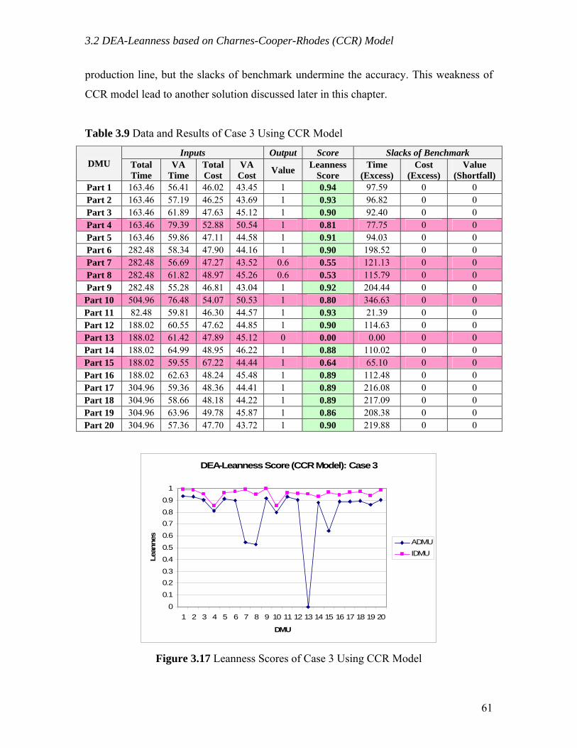
3.2 DEA-Leanness based on Charnes-Cooper-Rhodes (CCR) Model
production line, but the slacks of benchmark undermine the accuracy. This weakness of
CCR model lead to another solution discussed later in this chapter.
Table 3.9 Data and Results of Case 3 Using CCR Model
Inputs Output Score Slacks of Benchmark DMU Total
Time VA
Time Total Cost
VA Cost Value Leanness
Score Time
(Excess) Cost
(Excess) Value
(Shortfall) Part 1 163.46 56.41 46.02 43.45 1 0.94 97.59 0 0 Part 2 163.46 57.19 46.25 43.69 1 0.93 96.82 0 0 Part 3 163.46 61.89 47.63 45.12 1 0.90 92.40 0 0 Part 4 163.46 79.39 52.88 50.54 1 0.81 77.75 0 0 Part 5 163.46 59.86 47.11 44.58 1 0.91 94.03 0 0 Part 6 282.48 58.34 47.90 44.16 1 0.90 198.52 0 0 Part 7 282.48 56.69 47.27 43.52 0.6 0.55 121.13 0 0 Part 8 282.48 61.82 48.97 45.26 0.6 0.53 115.79 0 0 Part 9 282.48 55.28 46.81 43.04 1 0.92 204.44 0 0 Part 10 504.96 76.48 54.07 50.53 1 0.80 346.63 0 0 Part 11 82.48 59.81 46.30 44.57 1 0.93 21.39 0 0 Part 12 188.02 60.55 47.62 44.85 1 0.90 114.63 0 0 Part 13 188.02 61.42 47.89 45.12 0 0.00 0.00 0 0 Part 14 188.02 64.99 48.95 46.22 1 0.88 110.02 0 0 Part 15 188.02 59.55 67.22 44.44 1 0.64 65.10 0 0 Part 16 188.02 62.63 48.24 45.48 1 0.89 112.48 0 0 Part 17 304.96 59.36 48.36 44.41 1 0.89 216.08 0 0 Part 18 304.96 58.66 48.18 44.22 1 0.89 217.09 0 0 Part 19 304.96 63.96 49.78 45.87 1 0.86 208.38 0 0 Part 20 304.96 57.36 47.70 43.72 1 0.90 219.88 0 0
DEA-Leanness Score (CCR Model): Case 3
0
0.1
0.20.3
0.4
0.5
0.6
0.70.8
0.9
1
1 2 3 4 5 6 7 8 9 10 11 12 13 14 15 16 17 18 19 20
DMU
Lean
nes
ADMUIDMU
Figure 3.17 Leanness Scores of Case 3 Using CCR Model
61
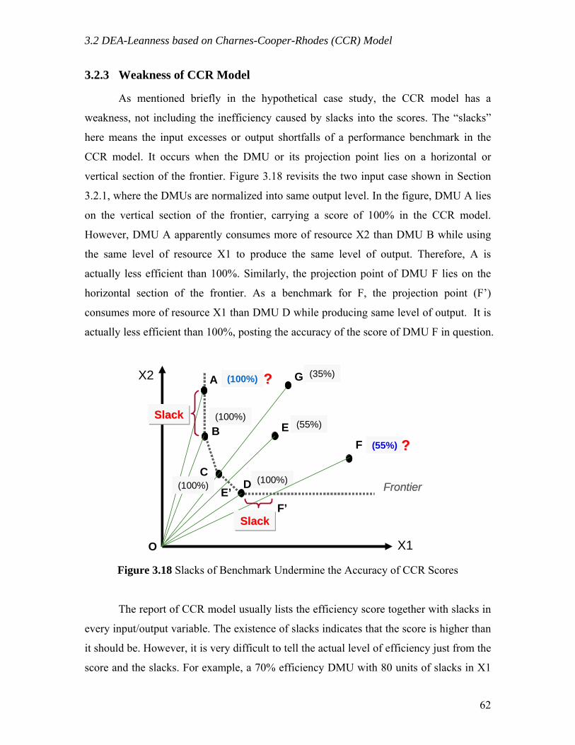
3.2 DEA-Leanness based on Charnes-Cooper-Rhodes (CCR) Model
3.2.3 Weakness of CCR Model
As mentioned briefly in the hypothetical case study, the CCR model has a
weakness, not including the inefficiency caused by slacks into the scores. The “slacks”
here means the input excesses or output shortfalls of a performance benchmark in the
CCR model. It occurs when the DMU or its projection point lies on a horizontal or
vertical section of the frontier. Figure 3.18 revisits the two input case shown in Section
3.2.1, where the DMUs are normalized into same output level. In the figure, DMU A lies
on the vertical section of the frontier, carrying a score of 100% in the CCR model.
However, DMU A apparently consumes more of resource X2 than DMU B while using
the same level of resource X1 to produce the same level of output. Therefore, A is
actually less efficient than 100%. Similarly, the projection point of DMU F lies on the
horizontal section of the frontier. As a benchmark for F, the projection point (F’)
consumes more of resource X1 than DMU D while producing same level of output. It is
actually less efficient than 100%, posting the accuracy of the score of DMU F in question.
(100%)
(100%)
(100%)
(55%)
(55%)
FrontierFrontier
A
BF
X1
E
CD
X2
E’F’
O
(35%)G
(100%)
SlackSlack
SlackSlack
?
??
?
Figure 3.18 Slacks of Benchmark Undermine the Accuracy of CCR Scores
The report of CCR model usually lists the efficiency score together with slacks in
every input/output variable. The existence of slacks indicates that the score is higher than
it should be. However, it is very difficult to tell the actual level of efficiency just from the
score and the slacks. For example, a 70% efficiency DMU with 80 units of slacks in X1
62

3.2 DEA-Leanness based on Charnes-Cooper-Rhodes (CCR) Model
may or may not be more comparable with a 60% efficient DMU with 50 units of slacks
in X1. Even slacks in different variable have different units. Therefore, a report of CCR
model becomes hard to comprehend when slacks exist.
From the three hypothetical cases, it appears that IDMUs tend to cluster at a small
area which leaves most of the frontier in vertical or horizontal sections. Therefore, slacks
are found repeatedly in every hypothetical case which can be observed in Figure 3.12,
3.14, and 3.16. The reason behind is that the VA activities in a manufacturing system
consumes similar amounts of cost and time, while NVA activities are usually the sources
of variability and are responsible for the larger portion of the total cost and time. Table
3.10 collects four examples of Value Stream Maps to compare the Lead Time and VA
Time of current state and future state. The results support that VA time does not change
much when a system is improved from current state to the proposed future state.
Similarly, Table 3.11 lists the costs and earnings of current and future states of the third
example. The conversion cost, which makes up most of the VA time, does not decrease
much, while the greatest improvement comes from the reduction of inventory value.
Table 3.10 Current and Future Value Stream Maps Have Similar VA Times
Example 1 Example 2 Example 3 Example 4 Lead Time 23.6 days 48 days 20.5 days 34 days Current
VSM VA Time 188 sec. 315 sec. 30.3 min. 170 sec. Lead Time 4.5 days 11 days 4.5 days 8 days Future
VSM VA Time 169 sec. 315 sec. 23.3 min. 150 sec.
Source Examples 1 and 2: “Learning to See” (Rother and Shooks, 1998) Example 3: “Practical Lean Accounting” (Maskell and Baggaley, 2003) Example 4: “Value Stream Management” (Tapping et al., 2002)
Table 3.11 Current and Future Value Stream Maps Have Similar VA Costs
Example 3 Current State Future State Inventory Value $58,502 $13,997
Revenue $1,292,640 $1,292,640 Material Costs $512,160 $447,160
Conversion Costs $189,866 $181,416 Value Stream Profit $590,614 $634,064
63
3.3 DEA-Leanness based on Slacks-Based Measure (SBM)
In summary, slacks can be found frequently in the DEA-Leanness Measure when
applied on manufacturing systems due to the cluster of IDMUs. The CCR model is
capable of evaluating the leanness level, but the result is not intuitively understandable.
The DEA-Leanness Measure should employ another model that delivers leanness scores
considering the inefficiency caused by slacks. A better solution is the Slacks-Based
Measure (SBM) model introduced in the following section.
3.3 DEA-Leanness based on Slacks-Based Measure (SBM)
Due to the weakness of CCR model on handling slacks, finding a more suitable
model for the DEA-Leanness Measure is necessary. The model of Slacks-Based Measure
(SBM) is selected to be the replacement since it is designed to deal with slacks directly.
The hypothetical cases are revisited in this section using the SBM model, and the results
are satisfying. Therefore, the SBM model is a better choice than CCR model while
performing the DEA-Leanness Measure.
3.3.1 Slacks-Based Measure (SBM) Model
The Slacks-Based Measure (SBM) of efficiency is proposed by Tone (2001) as a
DEA model that deals with the slacks in the input and output variables directly. Using the
input excesses and output shortfalls between a DMU and its benchmark, the SBM model
gives an efficiency score that is unit invariant and valued between 0 and 1. As shown
below, the original SBM model is also a fractional program. An equivalent linear
program can be derived using the similar transformation of the CCR model.
64
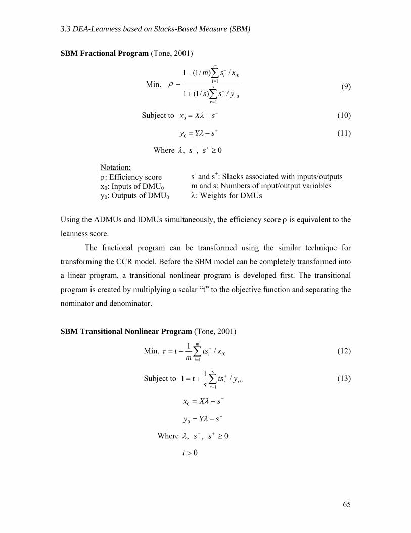
3.3 DEA-Leanness based on Slacks-Based Measure (SBM)
SBM Fractional Program (Tone, 2001)
Min. ∑
∑
=
+
=
−
+
−= s
rrr
m
iii
yss
xsm
10
10
/)/1(1
/)/1(1ρ (9)
Subject to (10) −+= sXx λ0
(11) +−= sYy λ0
Where 0,, ≥+− ssλ
Notation: ρ: Efficiency score x0: Inputs of DMU0y0: Outputs of DMU0
s- and s+: Slacks associated with inputs/outputs m and s: Numbers of input/output variables λ: Weights for DMUs
Using the ADMUs and IDMUs simultaneously, the efficiency score ρ is equivalent to the
leanness score.
The fractional program can be transformed using the similar technique for
transforming the CCR model. Before the SBM model can be completely transformed into
a linear program, a transitional nonlinear program is developed first. The transitional
program is created by multiplying a scalar “t” to the objective function and separating the
nominator and denominator.
SBM Transitional Nonlinear Program (Tone, 2001)
Min. ∑=
−−=m
iii xts
mt
10/1τ (12)
Subject to ∑=
++=s
rrr yts
st
10/11 (13)
−+= sXx λ0
+−= sYy λ0
Where 0,, ≥+− ssλ
0>t
65
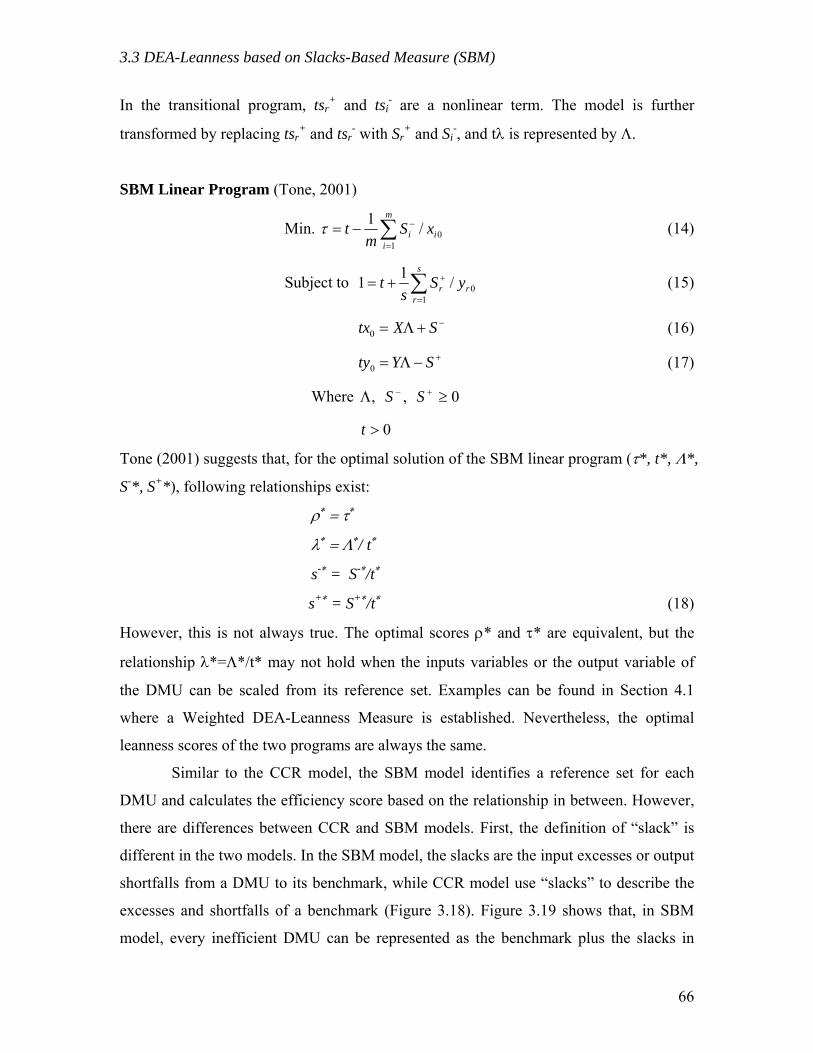
3.3 DEA-Leanness based on Slacks-Based Measure (SBM)
In the transitional program, tsr+ and tsi
- are a nonlinear term. The model is further
transformed by replacing tsr+ and tsr
- with Sr+ and Si
-, and tλ is represented by Λ.
SBM Linear Program (Tone, 2001)
Min. ∑=
−−=m
iii xS
mt
10/1τ (14)
Subject to ∑=
++=s
rrr yS
st
10/11 (15)
(16) −+Λ= SXtx0
(17) +−Λ= SYty0
Where 0,, ≥Λ +− SS
0>t
Tone (2001) suggests that, for the optimal solution of the SBM linear program (τ*, t*, Λ*,
S-*, S+*), following relationships exist:
ρ∗ = τ∗
λ∗ = Λ∗/ t∗
s-∗ = S-∗/t∗
s+∗ = S+∗/t∗ (18)
However, this is not always true. The optimal scores ρ* and τ* are equivalent, but the
relationship λ*=Λ*/t* may not hold when the inputs variables or the output variable of
the DMU can be scaled from its reference set. Examples can be found in Section 4.1
where a Weighted DEA-Leanness Measure is established. Nevertheless, the optimal
leanness scores of the two programs are always the same.
Similar to the CCR model, the SBM model identifies a reference set for each
DMU and calculates the efficiency score based on the relationship in between. However,
there are differences between CCR and SBM models. First, the definition of “slack” is
different in the two models. In the SBM model, the slacks are the input excesses or output
shortfalls from a DMU to its benchmark, while CCR model use “slacks” to describe the
excesses and shortfalls of a benchmark (Figure 3.18). Figure 3.19 shows that, in SBM
model, every inefficient DMU can be represented as the benchmark plus the slacks in
66
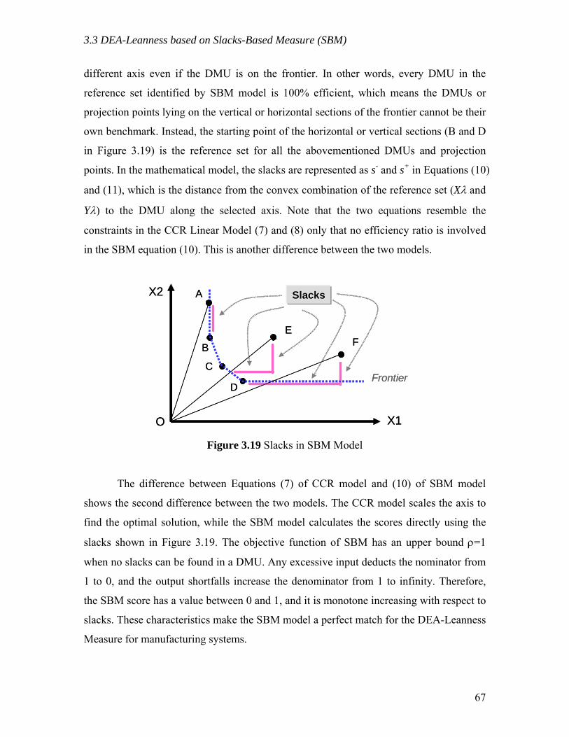
3.3 DEA-Leanness based on Slacks-Based Measure (SBM)
different axis even if the DMU is on the frontier. In other words, every DMU in the
reference set identified by SBM model is 100% efficient, which means the DMUs or
projection points lying on the vertical or horizontal sections of the frontier cannot be their
own benchmark. Instead, the starting point of the horizontal or vertical sections (B and D
in Figure 3.19) is the reference set for all the abovementioned DMUs and projection
points. In the mathematical model, the slacks are represented as s- and s+ in Equations (10)
and (11), which is the distance from the convex combination of the reference set (Xλ and
Yλ) to the DMU along the selected axis. Note that the two equations resemble the
constraints in the CCR Linear Model (7) and (8) only that no efficiency ratio is involved
in the SBM equation (10). This is another difference between the two models.
A
B FE
FrontierC
D
X1
X2 SlacksSlacks
O
A
B FE
FrontierC
D
X1
X2 SlacksSlacks
O Figure 3.19 Slacks in SBM Model
The difference between Equations (7) of CCR model and (10) of SBM model
shows the second difference between the two models. The CCR model scales the axis to
find the optimal solution, while the SBM model calculates the scores directly using the
slacks shown in Figure 3.19. The objective function of SBM has an upper bound ρ=1
when no slacks can be found in a DMU. Any excessive input deducts the nominator from
1 to 0, and the output shortfalls increase the denominator from 1 to infinity. Therefore,
the SBM score has a value between 0 and 1, and it is monotone increasing with respect to
slacks. These characteristics make the SBM model a perfect match for the DEA-Leanness
Measure for manufacturing systems.
67
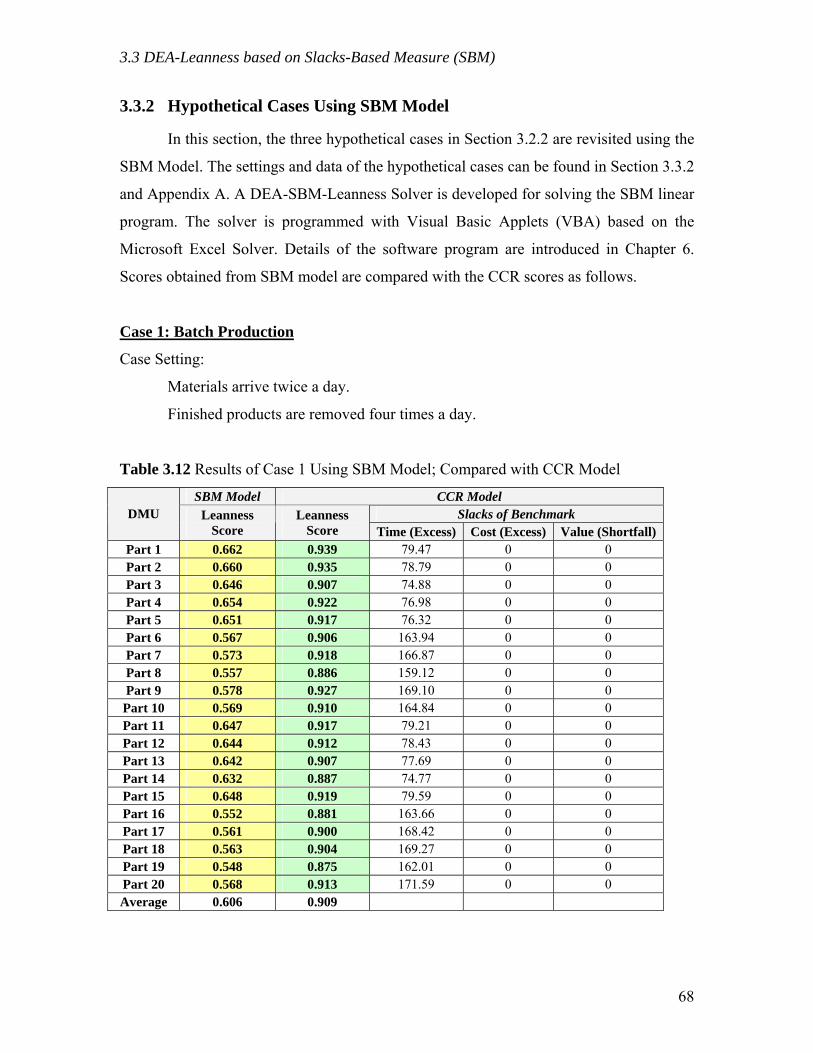
3.3 DEA-Leanness based on Slacks-Based Measure (SBM)
3.3.2 Hypothetical Cases Using SBM Model
In this section, the three hypothetical cases in Section 3.2.2 are revisited using the
SBM Model. The settings and data of the hypothetical cases can be found in Section 3.3.2
and Appendix A. A DEA-SBM-Leanness Solver is developed for solving the SBM linear
program. The solver is programmed with Visual Basic Applets (VBA) based on the
Microsoft Excel Solver. Details of the software program are introduced in Chapter 6.
Scores obtained from SBM model are compared with the CCR scores as follows.
Case 1: Batch Production
Case Setting:
Materials arrive twice a day.
Finished products are removed four times a day.
Table 3.12 Results of Case 1 Using SBM Model; Compared with CCR Model
SBM Model CCR Model Slacks of Benchmark DMU Leanness
Score Leanness
Score Time (Excess) Cost (Excess) Value (Shortfall) Part 1 0.662 0.939 79.47 0 0 Part 2 0.660 0.935 78.79 0 0 Part 3 0.646 0.907 74.88 0 0 Part 4 0.654 0.922 76.98 0 0 Part 5 0.651 0.917 76.32 0 0 Part 6 0.567 0.906 163.94 0 0 Part 7 0.573 0.918 166.87 0 0 Part 8 0.557 0.886 159.12 0 0 Part 9 0.578 0.927 169.10 0 0 Part 10 0.569 0.910 164.84 0 0 Part 11 0.647 0.917 79.21 0 0 Part 12 0.644 0.912 78.43 0 0 Part 13 0.642 0.907 77.69 0 0 Part 14 0.632 0.887 74.77 0 0 Part 15 0.648 0.919 79.59 0 0 Part 16 0.552 0.881 163.66 0 0 Part 17 0.561 0.900 168.42 0 0 Part 18 0.563 0.904 169.27 0 0 Part 19 0.548 0.875 162.01 0 0 Part 20 0.568 0.913 171.59 0 0 Average 0.606 0.909
68

3.3 DEA-Leanness based on Slacks-Based Measure (SBM)
Leanness Scores of Case 1
0.000
0.100
0.200
0.300
0.400
0.500
0.600
0.700
0.800
0.900
1.000
1 2 3 4 5 6 7 8 9 10 11 12 13 14 15 16 17 18 19 20
DMU
Lean
nes
SBM ScoresCCR Scores
Figure 3.20 Leanness Scores of Case 1: SBM Model vs. CCR Model
The result of Case 1 shows that the SBM Leanness Scores are significantly lower
than the CCR model. The production of 20 parts receives a score of 60.6%. The reason
for the difference is that CCR model does not include the slacks of benchmark in the
scores. More importantly, the hypothetical case is set to have four different batches of
products flowing through the production line. Due to the total time of the different
batches in the system, the ADMUs cluster into four groups as in Figure 3.12. The results
from SBM model successfully reflect the situation, while using CCR model, it can only
be observed from the value of slacks. Therefore, the SBM model provides a clearer
indication of the leanness of production which is simple and intuitive.
Case 2: Pull Production
Case Setting:
Materials are pulled only when needed.
Finished products are removed immediately after their completion.
The results from both SBM and CCR models are shown in Table 3.13 and Figure 3.21.
69
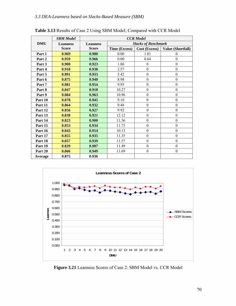
3.3 DEA-Leanness based on Slacks-Based Measure (SBM)
Table 3.13 Results of Case 2 Using SBM Model; Compared with CCR Model
SBM Model CCR Model Slacks of Benchmark DMU Leanness
Score Leanness
Score Time (Excess) Cost (Excess) Value (Shortfall) Part 1 0.969 0.980 0.00 1.01 0 Part 2 0.959 0.966 0.00 0.64 0 Part 3 0.908 0.923 1.86 0 0 Part 4 0.918 0.938 2.57 0 0 Part 5 0.891 0.933 5.42 0 0 Part 6 0.875 0.940 8.98 0 0 Part 7 0.881 0.954 9.93 0 0 Part 8 0.847 0.918 10.27 0 0 Part 9 0.884 0.963 10.96 0 0 Part 10 0.878 0.945 9.10 0 0 Part 11 0.864 0.932 9.48 0 0 Part 12 0.856 0.927 9.92 0 0 Part 13 0.838 0.921 12.12 0 0 Part 14 0.823 0.900 11.36 0 0 Part 15 0.853 0.934 11.73 0 0 Part 16 0.843 0.914 10.13 0 0 Part 17 0.855 0.935 11.35 0 0 Part 18 0.857 0.939 11.57 0 0 Part 19 0.829 0.907 11.49 0 0 Part 20 0.866 0.949 11.69 0 0 Average 0.875 0.936
Leanness Scores of Case 2
0.000
0.100
0.200
0.300
0.400
0.500
0.600
0.700
0.800
0.900
1.000
1 2 3 4 5 6 7 8 9 10 11 12 13 14 15 16 17 18 19 20
DMU
Lean
nes
SBM ScoresCCR Scores
Figure 3.21 Leanness Scores of Case 2: SBM Model vs. CCR Model
70
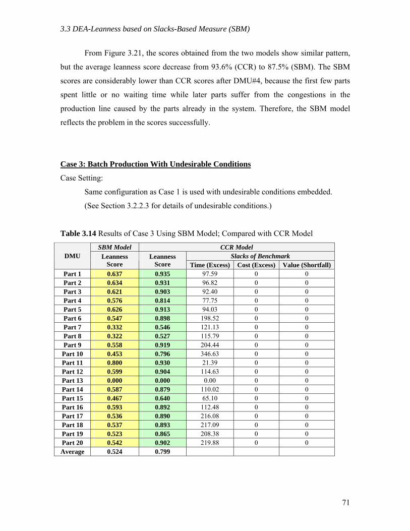
3.3 DEA-Leanness based on Slacks-Based Measure (SBM)
From Figure 3.21, the scores obtained from the two models show similar pattern,
but the average leanness score decrease from 93.6% (CCR) to 87.5% (SBM). The SBM
scores are considerably lower than CCR scores after DMU#4, because the first few parts
spent little or no waiting time while later parts suffer from the congestions in the
production line caused by the parts already in the system. Therefore, the SBM model
reflects the problem in the scores successfully.
Case 3: Batch Production With Undesirable Conditions
Case Setting:
Same configuration as Case 1 is used with undesirable conditions embedded.
(See Section 3.2.2.3 for details of undesirable conditions.)
Table 3.14 Results of Case 3 Using SBM Model; Compared with CCR Model
SBM Model CCR Model Slacks of Benchmark DMU Leanness
Score Leanness
Score Time (Excess) Cost (Excess) Value (Shortfall) Part 1 0.637 0.935 97.59 0 0 Part 2 0.634 0.931 96.82 0 0 Part 3 0.621 0.903 92.40 0 0 Part 4 0.576 0.814 77.75 0 0 Part 5 0.626 0.913 94.03 0 0 Part 6 0.547 0.898 198.52 0 0 Part 7 0.332 0.546 121.13 0 0 Part 8 0.322 0.527 115.79 0 0 Part 9 0.558 0.919 204.44 0 0 Part 10 0.453 0.796 346.63 0 0 Part 11 0.800 0.930 21.39 0 0 Part 12 0.599 0.904 114.63 0 0 Part 13 0.000 0.000 0.00 0 0 Part 14 0.587 0.879 110.02 0 0 Part 15 0.467 0.640 65.10 0 0 Part 16 0.593 0.892 112.48 0 0 Part 17 0.536 0.890 216.08 0 0 Part 18 0.537 0.893 217.09 0 0 Part 19 0.523 0.865 208.38 0 0 Part 20 0.542 0.902 219.88 0 0 Average 0.524 0.799
71

3.3 DEA-Leanness based on Slacks-Based Measure (SBM)
Leanness Scores of Case 3
0.000
0.100
0.200
0.300
0.400
0.500
0.600
0.700
0.800
0.900
1.000
1 2 3 4 5 6 7 8 9 10 11 12 13 14 15 16 17 18 19 20
DMU
Lean
nes
SBM ScoresCCR Scores
Figure 3.22 Leanness Scores of Case 3: SBM Model vs. CCR Model
In Case 3, the results from both models show a very similar pattern. The DMUs
with problems embedded receive lower leanness scores (i.e., Part #4, #7, #8, #10, #13
and #15). Again, SBM model gives lower score for every DMU because of the existence
of slacks in the CCR model. Among the DMUs, Part #11 receives significantly higher
score in the SBM model, which is not seen in the CCR model. From Figure 3.16 in
Section 3.2.2.3, Part #11 is the most efficient ADMU that locates near the cluster of
IDMUs in the Cost-Time space. Therefore, the SBM model correctly reflects the situation,
which is difficult to tell from the results of CCR model.
In summary, the hypothetical cases demonstrate the capability of DEA-Leanness
Measure on capturing the wastes and evaluating the leanness level of manufacturing
systems. CCR Model, the original DEA model, does not include the inefficiency caused
by slacks in the leanness score. This weakness limits the effectiveness of CCR model on
performing DEA-Leanness measuring since slacks are often found in general
manufacturing cases. The SBM model provides a solution to include all sources of
inefficiency into the leanness score and becomes a better choice for DEA-Leanness
Measure. The SBM model is used in all the other analyses in this research.
72
3.4 Contributions and Limitations of DEA-Leanness Measure
3.4 Contributions and Limitations of DEA-Leanness Measure
The proposed DEA-Leanness Measure provides a way to quantify the leanness
level of a manufacturing system based on a benchmark of ideal leanness obtained from
historical data. For lean practitioners, the leanness scores answer the question, “how lean
is the system?” Comparing to existing leanness assessment approaches, the development
of DEA-Leanness provides following specific contributions.
Contributions:
1) Integrated Index of Leanness: The first contribution of this research is to apply
DEA technique on measuring leanness. The leanness score derived by the DEA-
Leanness Measure provides an integrated index of leanness level of
manufacturing systems, which eliminates the need to interpret several lean metrics
at the same time. The score captures various types of wastes and provides a broad
picture of the level of leanness or waste of a system. The 0 to 1 unit-invariant
scale is easy to understand and efficient to compare between different
observations. It also provides the information of how much waste can be possibly
removed from the current system in order to reach ideal leanness.
2) Multiple Inputs: Most of the existing lean metrics consider either time-based
efficiency or cost efficiency only. The DEA-Leanness Measure considers the
investments on Cost and Time simultaneously as well as the output value of the
production effort.
3) Variable Scope of Application: For lean practitioners, different granulations of
value stream map are of interests during different stages of lean implementation.
Since the DEA-Leanness Measure utilizes the summations of cost, time and value,
it can be applied to a selected portion of a value stream regardless of the
configuration of the value stream. Measuring the leanness level of a complicated
value stream is made possible.
4) Self-contained Benchmark: Traditionally, lean practitioners rely on predefined
lean indicators or benchmarks from industrial group, published research or
consultants to evaluate their leanness. Using the DEA-Leanness Measure, the
73
3.4 Contributions and Limitations of DEA-Leanness Measure
frontier of leanness can be identified using historical data. The self-contained
benchmark eliminates the need to outsource for leanness benchmarks.
5) Up-to-date Frontier: The real frontier of leanness changes when technologies or
management skills improve. The leanness frontier obtained from the DEA-
Leanness Measure can be updated continuously when new data set is obtained.
6) Performance Standard: Comparing the DMUs having high or low leanness sore
may shed light on the performance standard for repeating production activities.
7) Directions of Improvements: The projection point of each ADMU on the
frontier provides a direction of possible improvement. The distance between an
ADMU and its benchmark suggests the extent of potential improvement in cost,
time and value (quality). Further investigation on the detailed processes is
required to form an actual improvement plan.
8) Tradeoffs between Competitive Strategies: The measure provides a potential on
helping decision makers to weight their competitive strategies. Improvements on
one variable often contradict the performance on other variables (e.g., time vs.
cost, value vs. cost, and time vs. value). The leanness measure provides
quantitative indices on how well the improvements are, or which strategy works
better.
In spite of the above contributions listed above, certain limitations associated with
the DEA-Leanness Measure are as follows.
Limitations:
1) Effectiveness of Leanness Frontier: Since there are potentially some
unidentifiable wastes (Figure 3.4), the frontier identified by DEA-Leanness
Measure may not be representing the true ideal leanness. A detailed and accurate
cost breakdown which identifies VA and NVA costs is required to improve the
quality of the frontier. Also, the ideal leanness changes over time, the cost
breakdown needs to be revaluated continuously.
2) Determining the Scope of Measurement: The scope of the leanness
measurement can be determined by the user of the model. It can be a
74
3.4 Contributions and Limitations of DEA-Leanness Measure
measurement for a workstation, a cell, a department, or a supply chain. However,
leanness of a section of a system does not represent the leanness of the whole
system. The scope of the measurement should be determined based on the needs
of the decision maker, and the results should be carefully interpreted based on the
chosen scope.
3) Leanness Target: Improving the system to achieve 100% appears to be the
ultimate goal for lean practitioners. However, there are some situations that make
this goal infeasible. A leanness target considering the unavoidable wastes would
be more reasonable. A methodology to identify a practical target can enhance the
application of the DEA-Leanness Measure.
4) Improvement of the Value Stream: The leanness measurement presents the
extent of potential improvements on cost and time investments of a current value
stream. However, the practical tactics to achieve these improvements are not
explicitly shown in the scores. Further investigations on the inefficiency of the
ADMUs are required to identify the practical actions of improvements.
5) Data Collection: The DEA-Leanness Measure compares the process of
producing each work piece in order to find the best leanness frontier. However,
collecting the detailed data of the production activities can be difficult.
Furthermore, large amount of data entry may lead to difficulty of solving the
mathematical model.
The limitations of the proposed DEA-Leanness Measure present some challenges
about the effectiveness of the measure, which nevertheless inspire more research ideas.
The following chapters introduce the extensions of the DEA-Leanness Measure,
including strategic tradeoffs, improvement identification, performance targeting, and the
software programs to carry out the leanness measure.
75
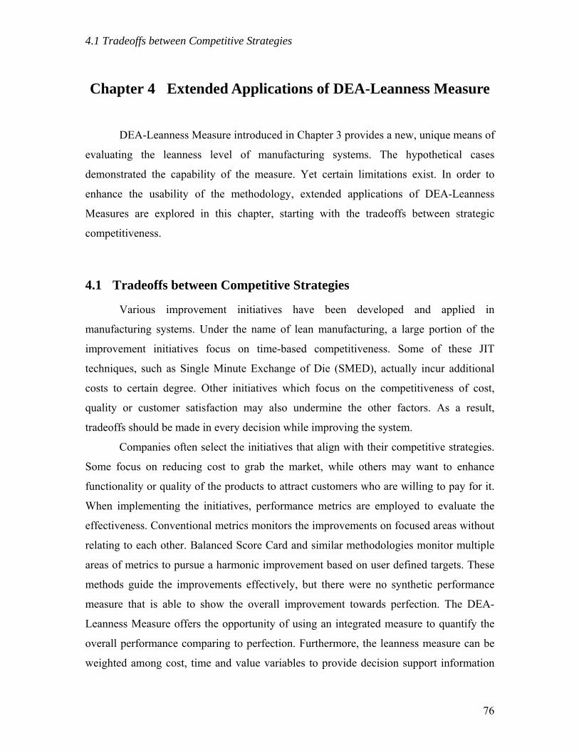
4.1 Tradeoffs between Competitive Strategies
Chapter 4 Extended Applications of DEA-Leanness Measure
DEA-Leanness Measure introduced in Chapter 3 provides a new, unique means of
evaluating the leanness level of manufacturing systems. The hypothetical cases
demonstrated the capability of the measure. Yet certain limitations exist. In order to
enhance the usability of the methodology, extended applications of DEA-Leanness
Measures are explored in this chapter, starting with the tradeoffs between strategic
competitiveness.
4.1 Tradeoffs between Competitive Strategies
Various improvement initiatives have been developed and applied in
manufacturing systems. Under the name of lean manufacturing, a large portion of the
improvement initiatives focus on time-based competitiveness. Some of these JIT
techniques, such as Single Minute Exchange of Die (SMED), actually incur additional
costs to certain degree. Other initiatives which focus on the competitiveness of cost,
quality or customer satisfaction may also undermine the other factors. As a result,
tradeoffs should be made in every decision while improving the system.
Companies often select the initiatives that align with their competitive strategies.
Some focus on reducing cost to grab the market, while others may want to enhance
functionality or quality of the products to attract customers who are willing to pay for it.
When implementing the initiatives, performance metrics are employed to evaluate the
effectiveness. Conventional metrics monitors the improvements on focused areas without
relating to each other. Balanced Score Card and similar methodologies monitor multiple
areas of metrics to pursue a harmonic improvement based on user defined targets. These
methods guide the improvements effectively, but there were no synthetic performance
measure that is able to show the overall improvement towards perfection. The DEA-
Leanness Measure offers the opportunity of using an integrated measure to quantify the
overall performance comparing to perfection. Furthermore, the leanness measure can be
weighted among cost, time and value variables to provide decision support information
76

4.1 Tradeoffs between Competitive Strategies
that is aligned with the company strategy. The impact of improvement initiatives and the
weighted measure are introduced in the following subsections.
4.1.1 Impacts of Improvement Initiatives
Different competitive strategies for manufacturing systems, such as Lean, Six
Sigma or Agile, often emphasize only part of the overall performance. Yet, the
improvement initiatives may have positive impacts on one performance area but have
negative impacts on the others. The DEA-Leanness Measure provides an opportunity to
evaluate the impact of an improvement initiative in terms of leanness level. Based on cost,
time and value, the leanness measure offers supporting information for decision makers
to judge the total effectiveness of the improvement initiatives and pinpoint the best
solution.
Time
Cost
AA
BB CC
DD
Current
Changes:AA: Time , Cost BB: Time , Cost CC: Time , Cost DD: Time , Cost
Figure 4.1 Changes from Current State in terms of Cost and Time
For a manufacturing system, the impacts of lean initiatives on cost and time can
be categorized as in Figure 4.1. From the current status, a system can be improved by
decreasing from one or both of the two dimensions. Therefore, sector A represents
improvement; sector C represents deterioration; while the impact of section B and D
depends on the amounts of the changes in the two axes. When the third axis, i.e., Value,
is considered, the rules change. The Value includes profit and all customer satisfaction
factors. Sector A can be deterioration if the value is decreased too much. On the other
hand, sector C can be an improvement if the value increased enough to justify the
increment in cost and time. As to B and D sectors, determination of the impact becomes
more complicated since all three factors need to be compared. These conditions for
improvements are summarized in Table 4.1.
77
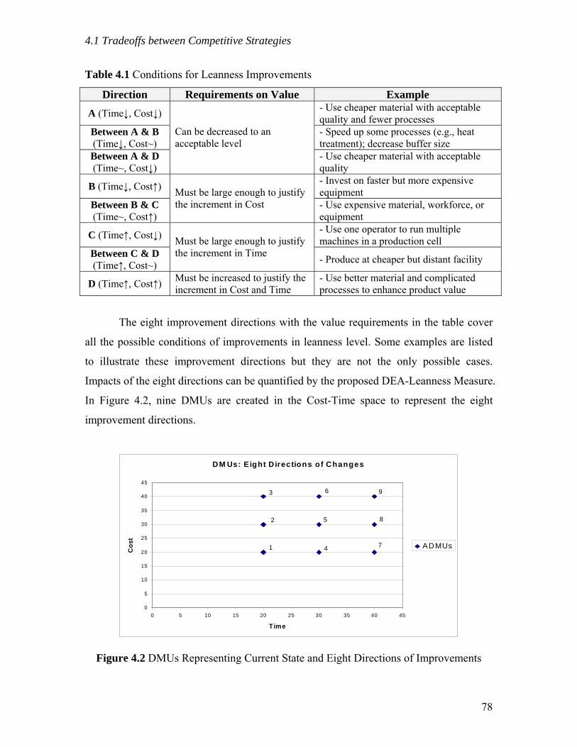
4.1 Tradeoffs between Competitive Strategies
Table 4.1 Conditions for Leanness Improvements
Direction Requirements on Value Example A (Time↓, Cost↓) - Use cheaper material with acceptable
quality and fewer processes Between A & B (Time↓, Cost~)
- Speed up some processes (e.g., heat treatment); decrease buffer size
Between A & D (Time~, Cost↓)
Can be decreased to an acceptable level
- Use cheaper material with acceptable quality
B (Time↓, Cost↑) - Invest on faster but more expensive equipment
Between B & C (Time~, Cost↑)
Must be large enough to justify the increment in Cost - Use expensive material, workforce, or
equipment
C (Time↑, Cost↓) - Use one operator to run multiple machines in a production cell
Between C & D (Time↑, Cost~)
Must be large enough to justify the increment in Time - Produce at cheaper but distant facility
D (Time↑, Cost↑) Must be increased to justify the increment in Cost and Time
- Use better material and complicated processes to enhance product value
The eight improvement directions with the value requirements in the table cover
all the possible conditions of improvements in leanness level. Some examples are listed
to illustrate these improvement directions but they are not the only possible cases.
Impacts of the eight directions can be quantified by the proposed DEA-Leanness Measure.
In Figure 4.2, nine DMUs are created in the Cost-Time space to represent the eight
improvement directions.
DM Us: Eight D irections of Changes
0
5
10
15
20
25
30
35
40
45
0 5 10 15 20 25 30 35 40 45
Time
Cos
t
ADMUs1
2
3
4
5
6
7
8
9
Figure 4.2 DMUs Representing Current State and Eight Directions of Improvements
78

4.1 Tradeoffs between Competitive Strategies
From the current state (DMU#5), the leanness level would be decreased while
moving to any other DMU. Three levels of output values (1.0, 0.75, and 0.5) are
employed to demonstrate the requirements of value associated with each direction. The
results are listed in Table 4.2 and also shown graphically in Figure 4.3.
Table 4.2 Leanness Scores of DMUs Representing Improvement Directions
Slacks DMUs Value Leanness
Score Time Cost Value 1 1.000 0.000 0.000 0.000 2 0.833 0.000 10.000 0.000 3 0.750 0.000 20.000 0.000 4 0.833 10.000 0.000 0.000 5 0.667 10.000 10.000 0.000 6 0.583 10.000 20.000 0.000 7 0.750 20.000 0.000 0.000 8 0.583 20.000 10.000 0.000 9
1.0
0.500 20.000 20.000 0.000 1 0.750 0.000 0.000 0.250 2 0.625 0.000 10.000 0.250 3 0.562 0.000 20.000 0.250 4 0.625 10.000 0.000 0.250 5 0.500 10.000 10.000 0.250 6 0.438 10.000 20.000 0.250 7 0.562 20.000 0.000 0.250 8 0.437 20.000 10.000 0.250 9
0.75
0.375 20.000 20.000 0.250 1 0.500 0.000 0.000 0.500 2 0.417 0.000 10.000 0.500 3 0.375 0.000 20.000 0.500 4 0.417 10.000 0.000 0.500 5 0.333 10.000 10.000 0.500 6 0.292 10.000 20.000 0.500 7 0.375 20.000 0.000 0.500 8 0.292 20.000 10.000 0.500 9
0.5
0.250 20.000 20.000 0.500
Consider DMU#5 with Value=0.75 as the original state, the other DMUs are the
eight directions of improvement, and the Value associated with each DMU plays a
79
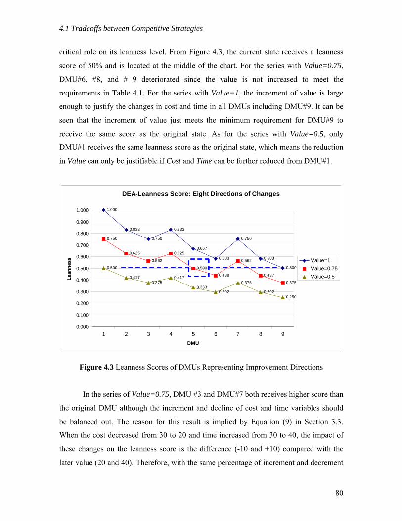
4.1 Tradeoffs between Competitive Strategies
critical role on its leanness level. From Figure 4.3, the current state receives a leanness
score of 50% and is located at the middle of the chart. For the series with Value=0.75,
DMU#6, #8, and # 9 deteriorated since the value is not increased to meet the
requirements in Table 4.1. For the series with Value=1, the increment of value is large
enough to justify the changes in cost and time in all DMUs including DMU#9. It can be
seen that the increment of value just meets the minimum requirement for DMU#9 to
receive the same score as the original state. As for the series with Value=0.5, only
DMU#1 receives the same leanness score as the original state, which means the reduction
in Value can only be justifiable if Cost and Time can be further reduced from DMU#1.
DEA-Leanness Score: Eight Directions of Changes
1.000
0.833
0.750
0.833
0.667
0.583
0.750
0.583
0.500
0.750
0.625
0.562
0.625
0.500
0.438
0.562
0.437
0.375
0.500
0.4170.375
0.417
0.3330.292
0.375
0.2920.250
0.000
0.100
0.200
0.300
0.400
0.500
0.600
0.700
0.800
0.900
1.000
1 2 3 4 5 6 7 8 9DMU
Lean
ness
Value=1Value=0.75Value=0.5
Figure 4.3 Leanness Scores of DMUs Representing Improvement Directions
In the series of Value=0.75, DMU #3 and DMU#7 both receives higher score than
the original DMU although the increment and decline of cost and time variables should
be balanced out. The reason for this result is implied by Equation (9) in Section 3.3.
When the cost decreased from 30 to 20 and time increased from 30 to 40, the impact of
these changes on the leanness score is the difference (-10 and +10) compared with the
later value (20 and 40). Therefore, with the same percentage of increment and decrement
80
4.1 Tradeoffs between Competitive Strategies
on each factor, the decrement has greater impact. The same result applies to the output
variable as well.
The example of improvement directions does not include IDMU to push the
frontier. As discussed in Section 3.2.3, the IDMUs usually do not improve much after
improvement initiatives since the VA cost and time normally do not decrease unless there
are dramatic technology advances. If the new IDMUs do push the frontier forward, then
the leanness scores of the original DMU need to be recalculated based on the new frontier.
Hence, the original and improved DMUs are always compared with each other based on
same standard.
In summary, the DEA-Leanness Measure provides a quantitative indication of the
impacts of improvement initiatives in terms of leanness level. The measure includes cost,
time and value as input/output variables and offers a synthesized, unit invariant leanness
score. However, in some situations, cost, time and value may not be taken as equally
important. Weighting the impacts of the changes of different variables allows calculation
of a leanness measure that better reflects the strategic plan.
4.1.2 Weighted DEA-Leanness Measure
In attempting to build profitable and sustainable companies, various strategies
have been developed and employed to keep a manufacturing system competitive. “Mass
Production” strategy, developed in the early 20th century, increases market share by
minimizing unit cost of a product. Time-based performance of the production and the
customers’ individual needs are often ignored under this strategy. The “Six Sigma”
methodology aims for preventing variability in a system to maximize quality of products.
The results include not only improved quality but also more stable lead time and less
unexpected costs. “Agile Manufacturing” stresses on rapid response to customers’
demand before competitors can react. Using this strategy, satisfying customers’
individual needs is most important, and higher unit cost or lead time is often justifiable.
As to “Lean Manufacturing,” it helps companies remove various types of waste from the
perspective of the customer’s viewpoint. Time-based performance is an important area of
lean implementation, but lean practitioners also benefit from lower overall cost, increased
81
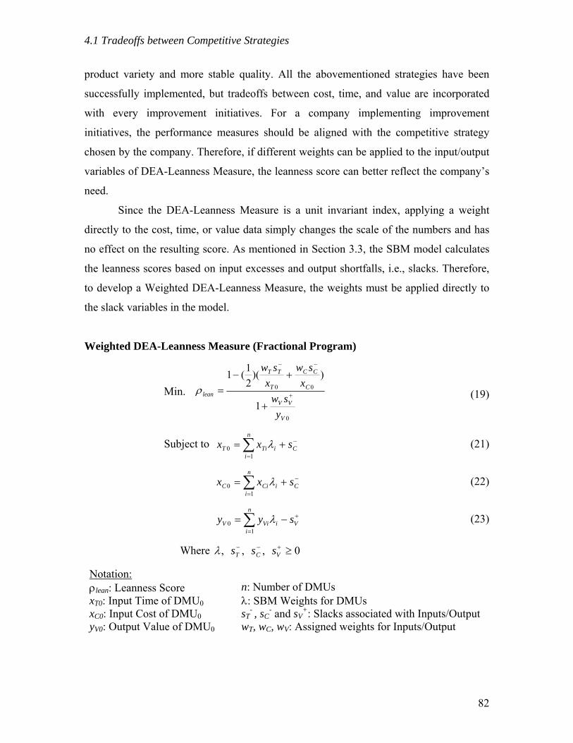
4.1 Tradeoffs between Competitive Strategies
product variety and more stable quality. All the abovementioned strategies have been
successfully implemented, but tradeoffs between cost, time, and value are incorporated
with every improvement initiatives. For a company implementing improvement
initiatives, the performance measures should be aligned with the competitive strategy
chosen by the company. Therefore, if different weights can be applied to the input/output
variables of DEA-Leanness Measure, the leanness score can better reflect the company’s
need.
Since the DEA-Leanness Measure is a unit invariant index, applying a weight
directly to the cost, time, or value data simply changes the scale of the numbers and has
no effect on the resulting score. As mentioned in Section 3.3, the SBM model calculates
the leanness scores based on input excesses and output shortfalls, i.e., slacks. Therefore,
to develop a Weighted DEA-Leanness Measure, the weights must be applied directly to
the slack variables in the model.
Weighted DEA-Leanness Measure (Fractional Program)
Min.
0
00
1
))(21(1
V
VV
C
CC
T
TT
lean
ysw
xsw
xsw
+
−−
+
+−=ρ (19)
Subject to (21) −
=
+= ∑ C
n
iiTiT sxx
10 λ
(22) −
=
+= ∑ C
n
iiCiC sxx
10 λ
(23) +
=
−= ∑ V
n
iiViV syy
10 λ
Where 0,,, ≥+−−VCT sssλ
Notation: ρlean: Leanness Score xT0: Input Time of DMU0xC0: Input Cost of DMU0yV0: Output Value of DMU0
n: Number of DMUs λ: SBM Weights for DMUs sT
- , sC
- and sV+: Slacks associated with Inputs/Output
wT, wC, wV: Assigned weights for Inputs/Output
82

4.1 Tradeoffs between Competitive Strategies
Similar to the original SBM model, the fractional program of the Weighted DEA-
Leanness Model can be transformed into an equivalent linear program by introducing a
multiplier t and defining the following relationships:
ST- = t sT
-, SC- = t sC
-, SV+ = t sV
-, and Λ = t λ.
Weighted DEA-Leanness Measure (Linear Program)
Min. ))(21(
00 C
CC
T
TTlean x
Swx
Swt−−
+−=τ (24)
Subject to 0
1V
VV
ySw
t+
+= (25)
(26) −
=
+Λ= ∑ T
n
iiTiT Sxtx
10
(27) −
=
+Λ= ∑ C
n
iiCiC Sxtx
10
(28) +
=
−Λ= ∑ V
n
iiViV Syty
10
Where 0,0,,, >≥Λ +−− tSSS VCT
As mentioned briefly in Section 3.3.1, Tone (2001) suggests that the optimal
solution set of the SBM fractional program (ρ*, λ*, s-*, s+*) is equal to (τ*, Λ*/ t*,
S-*/ t*, S+*/ t*). Based on this relationship, the transformation is deemed to be reversible
(Cooper et al., 2004, p.99). However, this relationship is not always true. The condition
λ*=Λ*/t* is not imposed in the model.
Consider the DMU#9 in Figure 4.2, the DMU consumes twice as much cost and
time of those of reference DMU #1. When the two DMUs deliver the same level of
output (let value=1), an optimal solution set of the SBM program can be derived:
Fractional Program: ρ*=0.5, sT-*=20, sC
-*=20, sV+*=0, and λ1*=1.
Linear Program: τ*=0.5, ST*-=20, SC-*=20, SV
+*=0, and Λ1*=1, where multiplier t*=1.
83
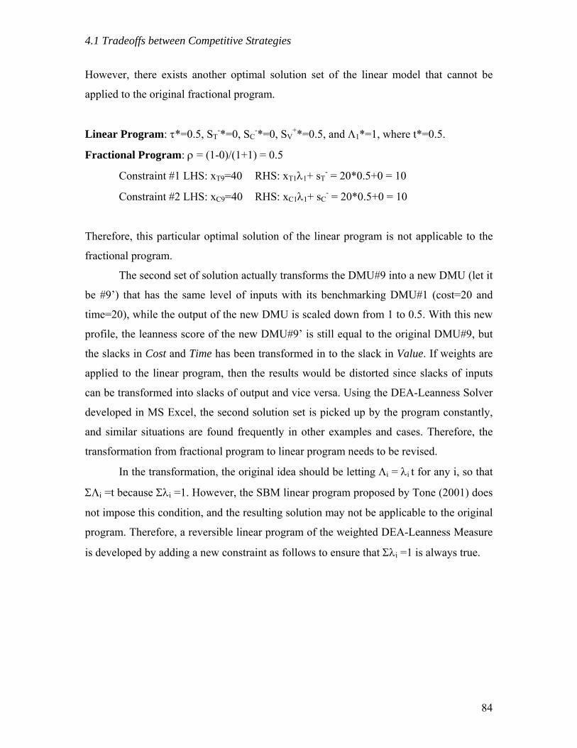
4.1 Tradeoffs between Competitive Strategies
However, there exists another optimal solution set of the linear model that cannot be
applied to the original fractional program.
Linear Program: τ*=0.5, ST-*=0, SC
-*=0, SV+*=0.5, and Λ1*=1, where t*=0.5.
Fractional Program: ρ = (1-0)/(1+1) = 0.5
Constraint #1 LHS: xT9=40 RHS: xT1λ1+ sT- = 20*0.5+0 = 10
Constraint #2 LHS: xC9=40 RHS: xC1λ1+ sC- = 20*0.5+0 = 10
Therefore, this particular optimal solution of the linear program is not applicable to the
fractional program.
The second set of solution actually transforms the DMU#9 into a new DMU (let it
be #9’) that has the same level of inputs with its benchmarking DMU#1 (cost=20 and
time=20), while the output of the new DMU is scaled down from 1 to 0.5. With this new
profile, the leanness score of the new DMU#9’ is still equal to the original DMU#9, but
the slacks in Cost and Time has been transformed in to the slack in Value. If weights are
applied to the linear program, then the results would be distorted since slacks of inputs
can be transformed into slacks of output and vice versa. Using the DEA-Leanness Solver
developed in MS Excel, the second solution set is picked up by the program constantly,
and similar situations are found frequently in other examples and cases. Therefore, the
transformation from fractional program to linear program needs to be revised.
In the transformation, the original idea should be letting Λi = λi t for any i, so that
ΣΛi =t because Σλi =1. However, the SBM linear program proposed by Tone (2001) does
not impose this condition, and the resulting solution may not be applicable to the original
program. Therefore, a reversible linear program of the weighted DEA-Leanness Measure
is developed by adding a new constraint as follows to ensure that Σλi =1 is always true.
84

4.1 Tradeoffs between Competitive Strategies
Weighted DEA-Leanness Measure (Reversible Linear Program)
Min. ))(21(
00 C
CC
T
TTlean x
Swx
Swt
−−
+−=τ
Subject to 0
1V
VV
ySw
t+
+=
−
=
+Λ= ∑ T
n
iiTiT Sxtx
10
−
=
+Λ= ∑ C
n
iiCiC Sxtx
10
+
=
−Λ= ∑ V
n
iiViV Syty
10
(29) ∑=
Λ=n
iit
1
Where 0,0,,, >≥Λ +−− tSSS VCT
Another issue of the Weighted DEA-Leanness Measure is that the weights applied
to the slacks cannot be assigned arbitrarily. In order to deliver a leanness score between 0
and 1, the weights for input slacks (wT and wC) must be summed up to 2, and the weight
for output slack (wV) must be adjusted accordingly. In other words, when a decision
maker ranks the relative importance of the three variables into a number, certain
calculation is required to translate the importance into applicable weights for the model.
Let the importance of Time, Cost and Value be represented by PT, PC, and PV,
respectively. The actual weights applied to the model are:
CT
TT PP
Pw+⋅
=2 (30)
CT
CC PP
Pw
+⋅
=2 (31)
CT
VV PP
Pw
+⋅
=2 (32)
The importance (PT, PC, and PV) can be determined by surveys or individual judgments
considering the strategic competitiveness. A simple solution is to assign a value scaled
85

4.1 Tradeoffs between Competitive Strategies
from 1 to 9 to each variable. For example, let PT=1, PC=3 and PV=2, the resulting weights
will be wT=0.5, wC=1.5, and wV=1 for the DEA model.
Some more delicate methodologies can be applied to determine the importance
level of the variables. For example, the Analytic Hierarchy Process (AHP) can synthesize
pair-wise relative importance levels (i.e., importance of Cost to Time, Time to Value and
Cost to Value) into a series of rationalized numbers between 0 and 1 with the sum equals
to 1 (Saaty, 1980). However, the process is developed for a large number of qualitative
decision variables. When few variables are involved, the conflicts between variables (e.g.,
PT=2PC, PC=2PV, and PV=2PT) can make the problem more complicated. In the DEA-
Leanness Measure, only three variables are involved. Therefore, the delicate
methodologies are not suggested for the determination of importance levels.
Using the DEA-Leanness Measure, the scores should be able to display the
impact of initiatives on the performance considering the company strategy. Using the
example of nine DMUs in Section 4.1.1again, the results of DEA-Leanness with different
weights are shown in the following figures.
Weighted DEA-Leanness Score
1.000
0.8890.833
0.778
0.6670.611
0.667
0.556
0.500
0.818
0.7270.682
0.636
0.5450.500
0.545
0.4550.409
0.600
0.5330.500
0.467
0.4000.367
0.400
0.3330.300
0.000
0.100
0.200
0.300
0.400
0.500
0.600
0.700
0.800
0.900
1.000
1 2 3 4 5 6 7 8 9DMU
Lean
ness
Value=1Value=0.75Value=0.5
Figure 4.4 Weighted Leanness Scores with PT=2, PC=1 and PV=1
86

4.1 Tradeoffs between Competitive Strategies
Weighted DEA-Leanness Score
1.000
0.778
0.667
0.889
0.667
0.556
0.833
0.611
0.500
0.818
0.636
0.545
0.727
0.545
0.455
0.682
0.500
0.409
0.600
0.467
0.400
0.533
0.400
0.333
0.500
0.367
0.300
0.000
0.100
0.200
0.300
0.400
0.500
0.600
0.700
0.800
0.900
1.000
1 2 3 4 5 6 7 8 9DMU
Lean
ness
Value=1Value=0.75Value=0.5
Figure 4.5 Weighted Leanness Scores with PT=1, PC=2 and PV=1
Weighted DEA-Leanness Score
1.000
0.833
0.750
0.833
0.667
0.583
0.750
0.583
0.500
0.600
0.5000.450
0.500
0.4000.350
0.450
0.3500.300
0.3330.278
0.2500.278
0.2220.194
0.2500.194
0.167
0.000
0.100
0.200
0.300
0.400
0.500
0.600
0.700
0.800
0.900
1.000
1 2 3 4 5 6 7 8 9DMU
Lean
ness
Value=1Value=0.75Value=0.5
Figure 4.6 Weighted Leanness Scores with PT=1, PC=1 and PV=2
87

4.2 DEA-Leanness Measure based on Existing Value Stream Maps
From the results, when the DEA-Leanness Measure is weighted as PT=2, PC=1
and PV=1 (Figure 4.4), the DMUs #4 to #9 receive lower scores than the original
condition due to the time slacks of these DMUs. Similarly, when the measure is weighted
as PT=1, PC=2 and PV=1 (Figure 4.5), the DMUs containing more costs than DMU#1
receive lower score than original condition. Finally in Figure 4.6, increasing the weight of
output Value affects the leanness score of DMUs in the second and third series, where
full value was not delivered.
The DEA-Leanness Measure gives an indication of the current performance
against perfection, and the weighted score aligns the performance measure with
competitive strategies. Simplified examples are created to demonstrate the use of DEA-
Leanness Measure and the weighted scores. In practice, the real cases may be much more
complicated, but the concept remains the same. The DEA-Leanness Measure provides
information to support decision makers in evaluating the improvement initiatives. When
weights are properly assigned, the leanness score can be applied to various manufacturing
strategies in addition to lean manufacturing.
4.2 DEA-Leanness Measure based on Existing Value Stream Maps
In the DEA-Leanness Measure, the whole production process of a work piece is
selected to be the DMU. Using the data of each work piece, individual differences, which
are ignored by average numbers, can be included. Thus, the virtual DMUs with the best
possible configuration are able to push the frontier as close as possible to the ideal
leanness. However, collecting data from all work pieces may require extra time and
efforts. Although a Web-based Kanban system is developed in this research (see Chapter
6) to facilitate the automatic data collection and analysis, in some cases, it may not be
practical to do so. One example is a large amount of work pieces flow through the
production line with high speed. Long and complicated production process, such as
products flowing through a long supply chain, is another example.
On the other hand, Value Stream Mapping, introduced by Rother and Shook
(1998), has become one of the most popular tools supporting lean implementation. It
88

4.2 DEA-Leanness Measure based on Existing Value Stream Maps
maps out the VA and NVA activities with remarks of time-based performance that
provide part of the information needed by the DEA-Leanness Measure. Although the
information contained in a traditional Value Stream Map (VSM) is not quite enough for
conducting the leanness measure, it should be a quick starting point if a few more
information can be added to complete the requirement. Due to the popularities of this
tool, many companies implementing lean manufacturing have built current state maps of
their manufacturing systems. Therefore, it should be convenient for them to evaluate their
leanness level by adding some extra data collected to their VSM instead of collecting
hundreds of data points from the shop floor. In this section, the possibility of applying
leanness measure based on VSM data is explored. The application in manufacturing
systems is discussed, which lead to a potential extension of this application to measuring
the overall leanness of a supply chain.
4.2.1 DEA-Leanness for Manufacturing Systems Using VSM
Value Stream Mapping has become one of the most popular techniques used by
lean practitioners. The technique is simple and intuitive to use and is very effective on
identifying wastes in the value stream. A typical VSM comes with time-based
performance, such as time in process, waiting in buffer, time in inventory, etc. An
example VSM of three VA activities is shown in Figure 4.7.
Unlike the Cost-Time-Value analysis (Chapter 3) where data is collected from
every work piece, the numbers associated with a VSM can be derived from aggregated
data. For example, the average processing time can be calculated as the total processing
time of a machine divided by the number of pieces processed by the machine. Similarly,
the amount of inventory divided by the daily demand represents the average time in
inventory. Collecting the aggregated data is usually more convenient than timing every
work piece. Therefore, obtaining the time averages for a VSM may require less effort
than collecting data from individual work pieces, and the averages are capable of
representing the general conditions of a value stream. However, an average value cannot
display the variability of the actual conditions. The lost information may contain clues of
the actual leanness level and potential improvements. If the DEA-Leanness Measure uses
89
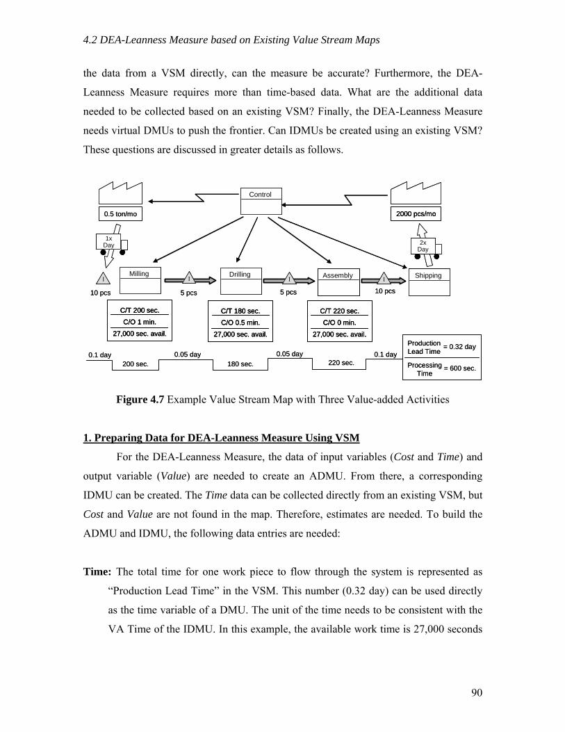
4.2 DEA-Leanness Measure based on Existing Value Stream Maps
the data from a VSM directly, can the measure be accurate? Furthermore, the DEA-
Leanness Measure requires more than time-based data. What are the additional data
needed to be collected based on an existing VSM? Finally, the DEA-Leanness Measure
needs virtual DMUs to push the frontier. Can IDMUs be created using an existing VSM?
These questions are discussed in greater details as follows.
ShippingDrilling AssemblyMillingI III
Control
2000 pcs/mo0.5 ton/mo
1xDay 2x
Day
5 pcs 5 pcs 10 pcs10 pcs
C/T 180 sec.
C/O 0.5 min.
27,000 sec. avail.
C/T 200 sec.
C/O 1 min.
27,000 sec. avail.
C/T 220 sec.
C/O 0 min.
27,000 sec. avail.
0.1 day 0.05 day 0.05 day 0.1 day200 sec. 180 sec. 220 sec.
ProductionLead Time
ProcessingTime
= 0.32 day
= 600 sec.
ShippingShippingDrillingDrilling AssemblyAssemblyMillingMillingI III
ControlControl
2000 pcs/mo2000 pcs/mo0.5 ton/mo
1xDay1x
Day 2xDay2x
Day
5 pcs 5 pcs 10 pcs10 pcs
C/T 180 sec.
C/O 0.5 min.
27,000 sec. avail.
C/T 180 sec.
C/O 0.5 min.
27,000 sec. avail.
C/T 200 sec.
C/O 1 min.
27,000 sec. avail.
C/T 200 sec.
C/O 1 min.
27,000 sec. avail.
C/T 220 sec.
C/O 0 min.
27,000 sec. avail.
C/T 220 sec.
C/O 0 min.
27,000 sec. avail.
0.1 day 0.05 day 0.05 day 0.1 day200 sec. 180 sec. 220 sec.
ProductionLead Time
ProcessingTime
= 0.32 day
= 600 sec.
Figure 4.7 Example Value Stream Map with Three Value-added Activities
1. Preparing Data for DEA-Leanness Measure Using VSM
For the DEA-Leanness Measure, the data of input variables (Cost and Time) and
output variable (Value) are needed to create an ADMU. From there, a corresponding
IDMU can be created. The Time data can be collected directly from an existing VSM, but
Cost and Value are not found in the map. Therefore, estimates are needed. To build the
ADMU and IDMU, the following data entries are needed:
Time: The total time for one work piece to flow through the system is represented as
“Production Lead Time” in the VSM. This number (0.32 day) can be used directly
as the time variable of a DMU. The unit of the time needs to be consistent with the
VA Time of the IDMU. In this example, the available work time is 27,000 seconds
90
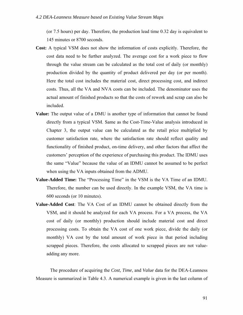
4.2 DEA-Leanness Measure based on Existing Value Stream Maps
(or 7.5 hours) per day. Therefore, the production lead time 0.32 day is equivalent to
145 minutes or 8700 seconds.
Cost: A typical VSM does not show the information of costs explicitly. Therefore, the
cost data need to be further analyzed. The average cost for a work piece to flow
through the value stream can be calculated as the total cost of daily (or monthly)
production divided by the quantity of product delivered per day (or per month).
Here the total cost includes the material cost, direct processing cost, and indirect
costs. Thus, all the VA and NVA costs can be included. The denominator uses the
actual amount of finished products so that the costs of rework and scrap can also be
included.
Value: The output value of a DMU is another type of information that cannot be found
directly from a typical VSM. Same as the Cost-Time-Value analysis introduced in
Chapter 3, the output value can be calculated as the retail price multiplied by
customer satisfaction rate, where the satisfaction rate should reflect quality and
functionality of finished product, on-time delivery, and other factors that affect the
customers’ perception of the experience of purchasing this product. The IDMU uses
the same “Value” because the value of an IDMU cannot be assumed to be perfect
when using the VA inputs obtained from the ADMU.
Value-Added Time: The “Processing Time” in the VSM is the VA Time of an IDMU.
Therefore, the number can be used directly. In the example VSM, the VA time is
600 seconds (or 10 minutes).
Value-Added Cost: The VA Cost of an IDMU cannot be obtained directly from the
VSM, and it should be analyzed for each VA process. For a VA process, the VA
cost of daily (or monthly) production should include material cost and direct
processing costs. To obtain the VA cost of one work piece, divide the daily (or
monthly) VA cost by the total amount of work piece in that period including
scrapped pieces. Therefore, the costs allocated to scrapped pieces are not value-
adding any more.
The procedure of acquiring the Cost, Time, and Value data for the DEA-Leanness
Measure is summarized in Table 4.3. A numerical example is given in the last column of
91
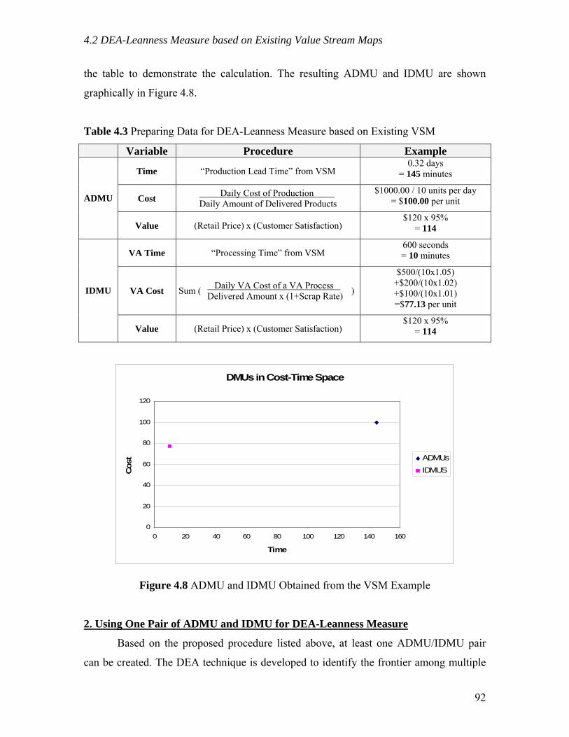
4.2 DEA-Leanness Measure based on Existing Value Stream Maps
the table to demonstrate the calculation. The resulting ADMU and IDMU are shown
graphically in Figure 4.8.
Table 4.3 Preparing Data for DEA-Leanness Measure based on Existing VSM
Variable Procedure Example
Time “Production Lead Time” from VSM 0.32 days
= 145 minutes
Cost Daily Cost of Production . Daily Amount of Delivered Products
$1000.00 / 10 units per day = $100.00 per unit ADMU
Value (Retail Price) x (Customer Satisfaction) $120 x 95%
= 114
VA Time “Processing Time” from VSM 600 seconds = 10 minutes
VA Cost Sum ( Daily VA Cost of a VA Process . Delivered Amount x (1+Scrap Rate) )
$500/(10x1.05) +$200/(10x1.02) +$100/(10x1.01) =$77.13 per unit
IDMU
Value (Retail Price) x (Customer Satisfaction) $120 x 95%
= 114
DMUs in Cost-Time Space
0
20
40
60
80
100
120
0 20 40 60 80 100 120 140 160
Time
Cos
t ADMUsIDMUS
Figure 4.8 ADMU and IDMU Obtained from the VSM Example
2. Using One Pair of ADMU and IDMU for DEA-Leanness Measure
Based on the proposed procedure listed above, at least one ADMU/IDMU pair
can be created. The DEA technique is developed to identify the frontier among multiple
92

4.2 DEA-Leanness Measure based on Existing Value Stream Maps
DMUs as a performance benchmark. When very few DMUs and multiple inputs/outputs
are considered, the original DEA model (i.e., CCR model) tends to form the frontier with
as many DMUs as possible. Therefore, with the only two DMUs, both of them may
receive a score of 100% lean. Fortunately, the SBM model is monotone increasing with
regards to slacks (input excesses or output shortfalls). From the definition, VA Time and
VA Cost cannot be greater than the Total Time and Total Cost. Therefore, unless the
ADMU is really 100% lean, the DEA-Leanness Measure using SBM model can always
capture the wastes of an ADMU and give a reasonable score. The results of the SBM
model are listed below.
Table 4.4 Leanness Score Derived from the VSM Example
Slack DMUs Leanness Score
Time Cost Value ADMU 0.420 135.000 22.870 0.000 IDMU 1.000 0.000 0.000 0.000
Actually, when only a pair of ADMU and IDMU is considered, the leanness score
of the ADMU can be calculated directly using Equation (9) without going through the
linear program. The calculation is listed below, which gives the same result as the SBM
model. Consequently, Equation (33) can be applied whenever only one ADMU/IDMU
pair is considered.
ADMU (xTA, xCA, yVA) = (145, 100, 114)
IDMU (xTI, xCI, yVI) = (10, 77.13, 114)
Leanness Score ))(
11(1
))(21(1
VA
VIVA
CA
CICA
TA
TITA
xxx
xxx
xxx
−+
−+
−−
= (33)
)114
114114)(11(1
)100
13.77100145
10145)(21(1
−+
−+
−−
=
= 0.420
93
4.2 DEA-Leanness Measure based on Existing Value Stream Maps
The pair of ADMU and IDMU is created based on the average time, cost, and
value of a selected time period. Using the same procedure, different pairs of ADMU and
IDMU can be created for different period of time. As a result, more than one pair of
DMUs can be created, and the average leanness level of different time windows can be
compared. However, the IDMUs are created using average number. The chance reaching
the ideal leanness by the IDMUs declines since the best configuration of DMUs has been
averaged out. The resulting leanness score may overestimate the actual leanness level
since the benchmark may not be lean enough.
3. Pushing the Frontier Further towards leanness
Since the average numbers may not be able to represent ideal leanness, the
leanness score may not be accurate. In order to ensure the quality of the frontier, the best
historical IDMUs forming the frontiers in the previous analysis should be included. A
rolling DEA approach is proposed in Section 4.4 to deal with the historical frontier DMU.
In this approach, the historical frontier is replaced by the new frontier if the later one is
leaner. Therefore, only the best DMUs of all time will be kept in the historical frontier
database. Using this approach, the frontier is guaranteed to be as good as that created
from previous DEA-Leanness analysis.
Beside historical data, leanness benchmark obtained externally can provide
valuable information. If an external benchmark is available and can be translated into a
DMU, it can provide an indication on how competitive the system can be in the market.
The problem with this method is that external benchmark is not always available or
trustworthy. This confirms an importance of using DEA technique that a self-contained
benchmark can always be identified.
Another way to acquire good IDMUs is actually sampling from the manufacturing
system. Although this section proposes a methodology to perform DEA-Leanness using
existing VSM without collecting actual data, sampling is an activity that is important for
all improvement techniques including VSM. The suggestion is to collect certain amount
of IDMUs from actual production periodically and then, use these IDMUs to ensure the
quality of the frontier in the later leanness analyses based on existing VSM.
94
4.2 DEA-Leanness Measure based on Existing Value Stream Maps
Other than the abovementioned methods, statistical techniques can be used to
identify a better frontier. It is much more complicated, since the distribution of the data
and some required statistics are unknown. Nevertheless, the resulting frontier may not be
reasonable if the estimates are incorrect. Therefore, the statistical techniques are not
recommended for forming the frontier further. With DEA technique, at least the frontier
is obtained from the data that are collected from real settings.
4.2.2 DEA-Leanness Measure for Supply Chain
The previous subsection discusses the potential use of DEA-Leanness Measure
based on existing VSM when data of individual work pieces is difficult to obtain.
Another situation where collecting individual data can be difficult is in the case of
complicated systems, such as a supply chain. When a product goes through many
distantly located facilities, collecting the detailed Cost, Time, and Value data becomes
cumbersome, let alone separating the VA and NVA inputs. Jones and Womack (2002)
apply the Value Stream Mapping technique on the Extended Value Stream, which is
actually a supply chain. The map is similar to the VSM for manufacturing system but
with wider scope and larger granulation. In the VSM for supply chain level, detailed
processes within a manufacturing facility are replaced by an icon with aggregated time-
based performance. Figure 4.9 shows a simplified example of the VSM for supply chain.
Similar to a detailed VSM, the line segments on the bottom of the map displays the
timeline of the whole supply chain operating process. The numbers above the upper lines
represent “Transportation Time.” Numbers above the lower lines are “In-plant Time”
with “Value Creating Time” in the brackets. Below the line segments, there are numbers
of the “Steps” involved during that period. These numbers are summarized in the data
boxes at both ends of the map.
95

4.2 DEA-Leanness Measure based on Existing Value Stream Maps
Warehouse
Control #1
1xWeek 1x
Day
1.0 day 5.0 d. 0.5 d. 1.0 day
2.5 d. (800 s.) 2.0 d. 2.0 d. (500 s.)
Control #2
Plant #1
MaterialSupplier
Plant #2
DistributionCenter
1xWeek
1xDay
3x Year
1000 m.Batch
=50 PalleteDefective
=5%
RM 30 h.
WIP 10 h.
FG 28 h.
115 (5)
13
110 (3)
1
RM 20 h.
WIP 10 h.
FG 15 h.
180 m.Batch
=10 PalleteDefective
=5%
400 m.Batch
=10 PalleteDefective
=1%
500 m.Batch
=50 PalleteDefective
=5% TransportTime
VATime
= 7.5 days
= 1300 sec.
TotalTIme
In-PlantTime = 6.5 days
= 14.0 days
TotalSteps
VASteps
= 8
= 32
WarehouseWarehouse
Control #1Control #1
1xWeek
1xWeek 1x
Day1x
Day
1.0 day 5.0 d. 0.5 d. 1.0 day
2.5 d. (800 s.) 2.0 d. 2.0 d. (500 s.)
Control #2Control #2
Plant #1
MaterialSupplier
Plant #2
DistributionCenter
1xWeek
1xWeek
1xDay1x
Day
3x Year
1000 m.Batch
=50 PalleteDefective
=5%
RM 30 h.
WIP 10 h.
FG 28 h.
115 (5)
13
110 (3)
1
RM 20 h.
WIP 10 h.
FG 15 h.
180 m.Batch
=10 PalleteDefective
=5%
400 m.Batch
=10 PalleteDefective
=1%
500 m.Batch
=50 PalleteDefective
=5% TransportTime
VATime
= 7.5 days
= 1300 sec.
TotalTIme
In-PlantTime = 6.5 days
= 14.0 days
TransportTime
VATime
= 7.5 days
= 1300 sec.
TotalTIme
In-PlantTime = 6.5 days
= 14.0 days
TotalSteps
VASteps
= 8
= 32
Figure 4.9 An Example of VSM for Supply Chain
For a product flowing through a supply chain, transportation and warehousing are
typically the activities that make up most of the total time. In this example, the total time
is 14 days, of which 7.5 days are transportation time and around 6.4 days are in-plant but
NVA time. Only 1,300 seconds (=21.67 minutes) are processing time that actually adds
value. It can be expected that the leanness level would be very low if these numbers are
plugged into the DEA-Leanness Measure directly. However, whether the transportation
time should be considered as non-value-adding is questionable?
According to Toyota Production System (Ohno, 1988), transportation is one of
the seven types of waste that should be eliminated. The lean manufacturing concepts
basically follow this rule and categorize transportation as non-value-added activity.
Indeed, in-plant transportation is not adding value, and it should be eliminated or
combined with value-added activities if possible. Outside the plant, scarce materials are
normally found in certain areas in the world, and companies with different specialties are
not necessarily located nearby. Without transportation, most industrial materials would
not be available, and the companies with different specialties would not be able to work
together. Therefore, transportation between different facilities may have to be considered
as value-adding.
96
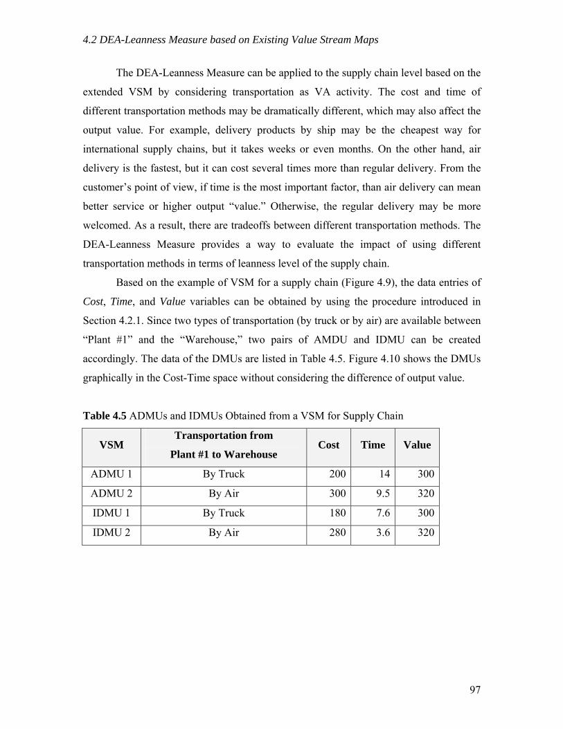
4.2 DEA-Leanness Measure based on Existing Value Stream Maps
The DEA-Leanness Measure can be applied to the supply chain level based on the
extended VSM by considering transportation as VA activity. The cost and time of
different transportation methods may be dramatically different, which may also affect the
output value. For example, delivery products by ship may be the cheapest way for
international supply chains, but it takes weeks or even months. On the other hand, air
delivery is the fastest, but it can cost several times more than regular delivery. From the
customer’s point of view, if time is the most important factor, than air delivery can mean
better service or higher output “value.” Otherwise, the regular delivery may be more
welcomed. As a result, there are tradeoffs between different transportation methods. The
DEA-Leanness Measure provides a way to evaluate the impact of using different
transportation methods in terms of leanness level of the supply chain.
Based on the example of VSM for a supply chain (Figure 4.9), the data entries of
Cost, Time, and Value variables can be obtained by using the procedure introduced in
Section 4.2.1. Since two types of transportation (by truck or by air) are available between
“Plant #1” and the “Warehouse,” two pairs of AMDU and IDMU can be created
accordingly. The data of the DMUs are listed in Table 4.5. Figure 4.10 shows the DMUs
graphically in the Cost-Time space without considering the difference of output value.
Table 4.5 ADMUs and IDMUs Obtained from a VSM for Supply Chain
VSM Transportation from
Plant #1 to Warehouse Cost Time Value
ADMU 1 By Truck 200 14 300
ADMU 2 By Air 300 9.5 320
IDMU 1 By Truck 180 7.6 300
IDMU 2 By Air 280 3.6 320
97
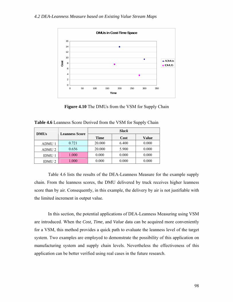
4.2 DEA-Leanness Measure based on Existing Value Stream Maps
DMUs in Cost-Time Space
0
2
4
6
8
10
12
14
16
0 50 100 150 200 250 300 350
Time
Cos
t ADMUsIDMUS
Figure 4.10 The DMUs from the VSM for Supply Chain
Table 4.6 Leanness Score Derived from the VSM for Supply Chain
Slack DMUs Leanness Score
Time Cost Value ADMU 1 0.721 20.000 6.400 0.000
ADMU 2 0.656 20.000 5.900 0.000
IDMU 1 1.000 0.000 0.000 0.000
IDMU 2 1.000 0.000 0.000 0.000
Table 4.6 lists the results of the DEA-Leanness Measure for the example supply
chain. From the leanness scores, the DMU delivered by truck receives higher leanness
score than by air. Consequently, in this example, the delivery by air is not justifiable with
the limited increment in output value.
In this section, the potential applications of DEA-Leanness Measuring using VSM
are introduced. When the Cost, Time, and Value data can be acquired more conveniently
for a VSM, this method provides a quick path to evaluate the leanness level of the target
system. Two examples are employed to demonstrate the possibility of this application on
manufacturing system and supply chain levels. Nevertheless the effectiveness of this
application can be better verified using real cases in the future research.
98

4.3 Identifying Potential Improvements Based on DEA-Leanness
4.3 Identifying Potential Improvements Based on DEA-Leanness
The DEA-Leanness Measure provides a way for lean practitioners to answer the
question: “how lean is the system?” Knowing the leanness level, the next question would
be “how to become leaner?” In other words, what are the wastes that can be removed
from the current system? Value Stream Mapping is a powerful tool for lean practitioners
to identify VA and NVA activities. A future state map created from the current condition
provides guidance for improvement actions. However, cost is not explicitly shown in the
map, and the time averages used in a VSM only display a general condition. The
individual differences of the production of each work piece may contain clues for further
improvement. In other words, if the DMU receiving the highest leanness score is
compared with the one receiving lowest score, the difference between the two DMUs
reveals the potential improvement directions. Yet, how to compare the DMUs becomes
the core question to be answered. The answer lies in the Cost-Time-Value analysis that is
proposed in Section 3.1.3 for data collection.
4.3.1 Cost-Time Profile (CTP) Analysis
The leanness level of a manufacturing system can be improved by decreasing cost
or time consumed by the process, or by improving the output value. In order to identify
the potential areas that can be improved, the cost and time consumed in the process and
the output value need to be compared. In Section 3.1.3, a Cost-Time-Value analysis is
introduced to prepare the input/output variables for each DMU. A Cost-Time-Value chart
(Figure 3.5) is used to illustrate the relationships between the three variables. This very
chart can be the tool to compare the cost, time and value data between DMUs and further
identify potential improvement areas. Actually, a very similar tool has been developed
and implemented a few decades ago. Before getting into the improvement identification,
the original tool is introduced first.
The Cost-Time Profiling technique was developed by Westinghouse in the 1970s
to “identify, understand, and quantify business process improvements” (Fooks, 1993).
With this technique, a Cost-Time Profile (CTP) maps out the monetary investment over
99

4.3 Identifying Potential Improvements Based on DEA-Leanness
the timeline of a production process (Rivera and Chen, 2006). Figure 4.11 shows a
sample CTP that demonstrates the components of a CTP.
In a CTP, the “Costs” are accumulated along the timeline of manufacturing
processes. A vertical segment of the profile represents the time-invariant investment
which happens all at once on a time spot, such as the arrival/addition of material or parts
in a production line. A slope represents a time-based investment, such as labor costs,
which increases over time. Horizontal segments are the waiting periods where no direct
costs are added during that period.
Time
Cost(Accumulated)
Wait
ActivityMaterial
TotalCost
Time
Cost(Accumulated)
Wait
ActivityMaterial
TotalCost
Figure 4.11 The Components of a Cost-Time Profile
When a CTP is built, the area under the curve, known as Cost-Time Investment
(CTI), represents the time-value of working capital that has been locked in this process
(Rivera and Chen, 2006). The CTI can be improved (decreased) by decreasing total cost,
shortening lead time, or simply postpone an activity or the arrival of material. A smaller
CTI value means more freedom of the working capital during that process, but it does not
necessarily mean less total cost or shorter lead time. Similar to the tradeoffs between cost
and time in the leanness measurement, when one of the two factors has been decreased to
a certain level, the increment in the other factor can be justifiable within an acceptable
range. As a result, the area under the curve can be decrease by cutting down from either
or both axes. Thus, the CTI value can be used to evaluate the impacts and tradeoffs of
improvement initiatives in terms of cost and time.
A CTP looks very similar to the Cost-Time-Value (CTV) chart in Figure 3.5, but
there are fundamental differences between the two charts.
100
4.3 Identifying Potential Improvements Based on DEA-Leanness
1) Output Value: The output value of the product is not included in the CTP. Therefore,
using a CTP, tradeoffs between improvements are only compared by cost and time or
the CTI without considering the impacts on value. The CTV analysis, on the other
hand, includes the output value for the DEA-Leanness Measure. The resulting scores
provide different information from the CTI area.
2) VA vs. NVA: The CTP does not differentiate VA and NVA activities explicitly. The
horizontal segments represent waiting, but the other types of NVA activities, such as
transportation, are not distinguished from the activities. The CTV chart distinguishes
VA activities from NVA activities, and also separates the VA costs from NVA costs
in order to create the IDMUs. The separated costs may provide more clues on
potential improvement directions.
3) Waiting Costs: The CTP includes material costs and direct costs in the curve.
Overhead is not included, so the waiting does not increase cost. In the CTV chart,
waiting still increases NVA cost over time.
CTP is a useful tool for identifying the time-value of monetary investment.
However, by separating VA and NVA costs, the charts may show more information of
the potential improvements on leanness. Hence, the CTV chart is suggested to be the tool
for DMU comparison.
4.3.2 Improvement Cycle Based on DEA-Leanness and CTV Chart
The leanness level of a manufacturing system can be improved by decreasing cost
or time, or increasing output value. In order to identify the potential improvement
directions, the CTV chart is employed to compare the three variables of DMUs. Figure
4.12 shows an example of a CTV chart that compares DMU#1 and #2. In the chart, VA
Costs and NVA Costs of the two DMUs are plotted as curves accumulating across the
production period. Leanness scores and output values are listed beside of the chart to
provide necessary information for the comparison. According to the scores, DMU#2 is
leaner than DMU#1, while the output values are similar. From the chart, DMU#2 uses
101

4.3 Identifying Potential Improvements Based on DEA-Leanness
apparently less time and a little less cost than DMU#1. Therefore, the second DMU
receives higher leanness score. Assume that DMU#2 is the best DMU among a batch.
The curves show that the DMU#1 spent more time on the first and last waiting period, so
this is the first potential improvement for this system. Also, DMU#2 uses less time on the
second process, which also leads to less time-based cost. This can be set as a performance
target for the later production, which can bring the leanness level of the later DMUs
closer to DMU#2. As such, the comparison of CTV charts between DMUs reveals
potential improvement directions and future performance targets.
Cost
Time
VA Cost of DMU#1
NVA Cost of DMU#1
Leanness ScoreDMU#1 = 0.71DMU#2 = 0.82
Output ValueDMU#1 = 95DMU#2 = 96
Leanness ScoreDMU#1 = 0.71DMU#2 = 0.82
Output ValueDMU#1 = 95DMU#2 = 96
VA Cost of DMU#2
NVA Cost of DMU#2
Cost
Time
VA Cost of DMU#1
NVA Cost of DMU#1
Leanness ScoreDMU#1 = 0.71DMU#2 = 0.82
Output ValueDMU#1 = 95DMU#2 = 96
Leanness ScoreDMU#1 = 0.71DMU#2 = 0.82
Output ValueDMU#1 = 95DMU#2 = 96
VA Cost of DMU#2
NVA Cost of DMU#2
Figure 4.12 Comparing DMUs in a CTV Chart
After the improvement actions are carried out, the leanness scores should be
monitored continuously to identify further improvement. The cycle of continuous
improvement using DEA-Leanness Score and CTV chart is summarized as follows.
1) Data Collection: Collects Cost, Time, and Value data to create ADMUs and IDMUs
for DEA-Leanness measurement.
2) Leanness Scores: Calculate leanness scores of the ADMUs and identify the ADMUs
with highest and lowest leanness scores.
3) CTV Comparison: Compare the best and worst ADMUs in a CTV chart. Selected
DMUs can be added to the chart for further comparison if necessary.
4) Wastes Identification: Identify the wastes by comparing the performance of DMUs
based on the VA and NVA curves in the chart. Wastes can be found when a DMU
102
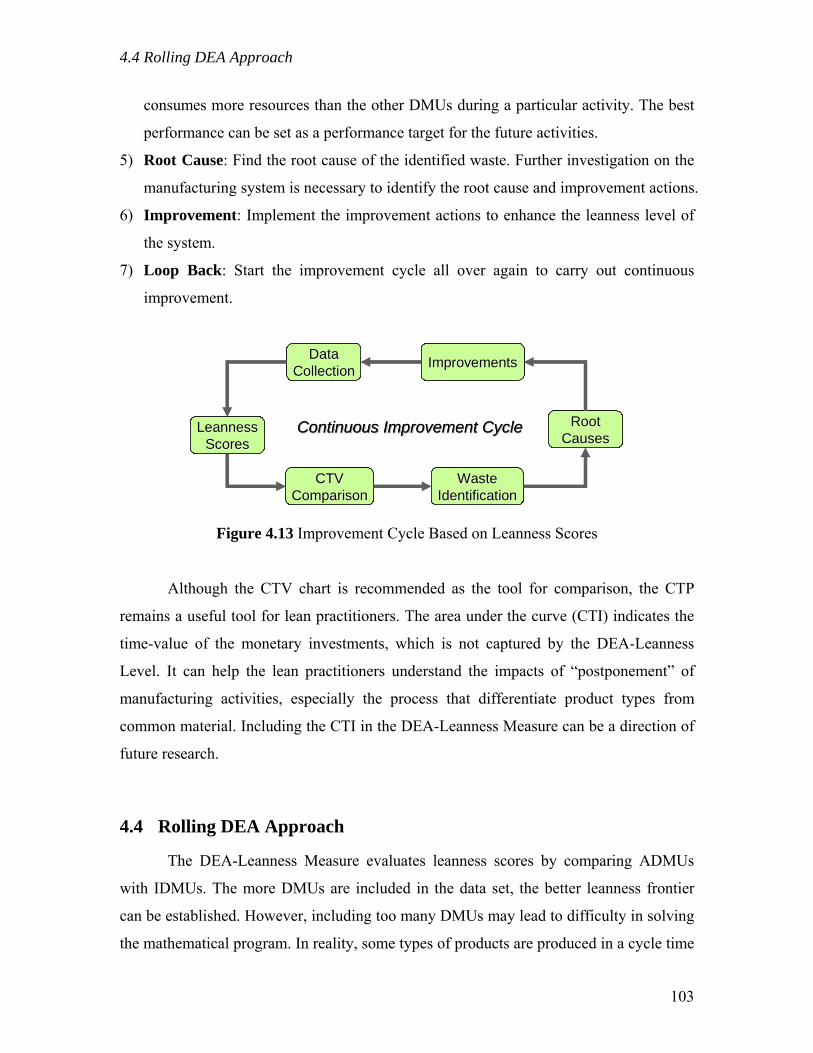
4.4 Rolling DEA Approach
consumes more resources than the other DMUs during a particular activity. The best
performance can be set as a performance target for the future activities.
5) Root Cause: Find the root cause of the identified waste. Further investigation on the
manufacturing system is necessary to identify the root cause and improvement actions.
6) Improvement: Implement the improvement actions to enhance the leanness level of
the system.
7) Loop Back: Start the improvement cycle all over again to carry out continuous
improvement.
DataDataCollectionCollection
CTVCTVComparisonComparison
WasteWasteIdentificationIdentification
RootRootCausesCauses
ImprovementsImprovements
Continuous Improvement CycleContinuous Improvement CycleLeannessLeannessScoresScores
DataDataCollectionCollection
CTVCTVComparisonComparison
WasteWasteIdentificationIdentification
RootRootCausesCauses
ImprovementsImprovements
Continuous Improvement CycleContinuous Improvement CycleLeannessLeannessScoresScores
Figure 4.13 Improvement Cycle Based on Leanness Scores
Although the CTV chart is recommended as the tool for comparison, the CTP
remains a useful tool for lean practitioners. The area under the curve (CTI) indicates the
time-value of the monetary investments, which is not captured by the DEA-Leanness
Level. It can help the lean practitioners understand the impacts of “postponement” of
manufacturing activities, especially the process that differentiate product types from
common material. Including the CTI in the DEA-Leanness Measure can be a direction of
future research.
4.4 Rolling DEA Approach
The DEA-Leanness Measure evaluates leanness scores by comparing ADMUs
with IDMUs. The more DMUs are included in the data set, the better leanness frontier
can be established. However, including too many DMUs may lead to difficulty in solving
the mathematical program. In reality, some types of products are produced in a cycle time
103

4.4 Rolling DEA Approach
as short as seconds. With this pace, thousands of ADMUs can be obtained from one day’s
production. Furthermore, creating corresponding IDMUs from ADMUs doubles the size
of a data set. As a result, setting up and solving the mathematical model for the DEA-
Leanness Measure may require a lot of extra efforts and time. In order to practically
implement the leanness measure, a Rolling DEA Approach is developed.
In most cases, only a few of the DMUs within a data set lies on the frontier. The
inefficient DMUs do not contribute to the formation of the frontier. Therefore, when any
of the inefficient DMUs is removed from the data set, the frontier is not affected and the
leanness scores of remaining DMUs also stay unchanged. On the other hand, if a new
DMU introduced to a data set is leaner than any existing DMU, the frontier will be
redefined by this new DMU. The leanness scores of all existing DMUs will then become
lower. Therefore, no matter how many DMUs are considered, the leanness scores are
determined by the most efficient ones of the whole data set. The following figure
demonstrates different frontiers enveloping Data Set 1, Data Set 2, and the combination
of the two data sets. Frontier 1 covers all DMUs in Data Set 1 but fails to cover some of
the DMUs in Data Set 2. Same situation happens to Frontier 2. The Overall Frontier is
defined by the most efficient DMUs from both data sets, and consequently, all the DMUs
are enveloped by this frontier.
Cost
Time: Data Set 1
: Data Set 2
Frontier 1
Frontier 2
Cost
Time Frontier 2: Data Set 1
: Data Set 2
Frontier 1OverallFrontierOverallFrontier
Figure 4.14 Frontiers Obtained from Different Data Sets
104

4.4 Rolling DEA Approach
Based on this observation, a Rolling DEA approach is developed to ease the
computation of a large number of DMUs. This approach maintains a group of Historical
Frontier DMUs (the DMUs forming the previous frontiers) collected from previous DEA
runs. As shown in Figure 4.15, every time a new data set is to be evaluated, the Historical
Frontier DMUs are evaluated together with the new DMUs by the DEA-Leanness
Measure. Therefore, the resulting frontier of the new data set is guaranteed to be as good
as previous frontiers. If the new data set contains better DMUs than the Historical
Frontier DMUs, the DMUs forming the new frontier are added to the database of
Historical Frontier DMUs while the less efficient historical DMUs are removed from the
database. Thus, whenever a data set is evaluated by the DEA-Leanness Measure, the
resulting frontier is the closest one to the ideal leanness that can be defined from the
existing knowledge.
DataSet
ADMUs
IDMUs
NewFrontier
LeannessScores
DEALModel
HistoricalFrontierDMUs
Figure 4.15 The Concept of Rolling DEA Approach
The Rolling DEA approach facilitates the process of DEA-Leanness measurement
when new data sets are obtained from the manufacturing systems. Including the up-to-
date Historical Frontier DMUs in every measuring process ensures the effectiveness of
the leanness benchmark. In Chapter 5, it is shown that the Rolling DEA approach also
105

4.4 Rolling DEA Approach
makes the calculation of leanness target easier since only the DMU for leanness target is
compared to Historical Frontier DMUs.
Another situation where Rolling DEA approach can be used is when a data set is
too large to be solved at once. For example, the DEA Solver provided by SAITECH used
in Section 3.2 can only handle 50 DMUs at once. Data set larger than 50 DMUs needs to
be solved using the Rolling DEA approach. A large data set can be divided into smaller
groups of data and solved separately. After solving all the data groups, the DMUs
forming the frontier of each data group are all included in the Historical Frontier database.
Following that, each of the data group is solved again together with the Historical
Frontier DMUs. The resulting leanness scores are exactly the same as solving the whole
data set all together.
The Rolling DEA technique is extremely important for tracking the progress of
leanness improvement in a manufacturing system. When production technologies and
management skills improve gradually, the benchmark of leanness should be updated
accordingly. In order to compare the old data and new data on the same ground, the
scores of old data sets need to be recalculated against the up-to-date frontier every time.
Instead of including all data sets into a huge mathematical program, the Rolling DEA
approach can recalculate the scores of every data set easily. This relaxes the requirement
of computational power while keeping the same quality of output scores.
In the literature review of DEA in Chapter 2, a Window Analysis technique has
been discussed. Similar to the Rolling DEA approach, this technique is developed to
demonstrate the changes of efficiency over certain periods of time. Instead of computing
efficiency scores against same frontier, the Window Analysis compares the performance
of a set of systems observed in different time frames, which are the Windows of time. As
a result, different frontiers are determined for different time frames. An efficiency score
shows the performance of an observed system (i.e., a DMU) within a certain Window,
and several Windows are compared to demonstrate the changes of comparative
performance of a DMU over a period of time. Therefore the Window Analysis can be
used to identify the leaders of DMUs (in terms of performance) over a time span and rank
the rest of the DMUs. However, the efficiency scores in different time frames are not
comparable since they are derived from different standard. As a result, the Window
106

4.4 Rolling DEA Approach
Analysis cannot be used in the DEA-Leanness Measure due to the inconsistency of the
standards. On the other hand, the Rolling DEA approach compares every data set using
the same standard as long as the Historical Frontier is maintained appropriately. It
supports the DEA-Leanness Measure on the comparison over time.
107
5.1 Ultimate Leanness versus Acceptable Leanness Level
Chapter 5 An Integrated Lean-Agile Performance Index
For lean practitioners, pursuing perfection is the goal of lean implementation. The
DEA-Leanness Measure indicates “how much leaner” the system can be. Yet, a “perfect”
manufacturing system without any waste is not likely to exist in reality. 100% leanness
may not be the answer to the question of “how lean the system should be.” This chapter
proposes a methodology to identify an appropriate leanness target for lean practitioners.
The leanness level of current system can be compared with this target to determine
whether it is “lean enough.” Hypothetical cases are included in this chapter to verify the
proposed methodology.
5.1 Ultimate Leanness versus Acceptable Leanness Level
The DEA-Leanness Measure provides an indication of perfection (continuous
improvement). It shows how much a system can be improved from its current state to a
near-perfect state. For a manufacturing system, the ideal leanness can be achieved by pull
production with one-piece (or continuous) flow moving through a fully synchronized
production line without any breakdown, quality problem or operational variability.
Beside of the ideal condition within the system, the demand of product and supply of
material must be extremely steady to avoid accumulating inventory in any stage of the
system. Only if all the perfect conditions exist simultaneously can the system achieve this
100% leanness.
In reality, the above mentioned ideal situation is nonexistent. Various kinds of
problems occurring in real life cause wastes in the system that lower the leanness score.
Thus, the ultimate leanness may not be a practical target for real manufacturing systems.
In the development and implementation of lean manufacturing, various tools and
methodologies have been developed to prevent the undesirable conditions from
happening. For example, the Total Productive Maintenance (TPM) is developed to
enhance productivity by avoiding wastes caused by failures of equipment; a “Poka Yoke”
(mistake proof) design avoids human errors; one of the benefits of implementing “5S” in
Toyota Production System is to prevent from wasting time on finding things when they
108
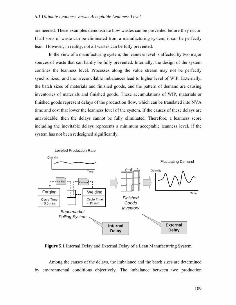
5.1 Ultimate Leanness versus Acceptable Leanness Level
are needed. These examples demonstrate how wastes can be prevented before they occur.
If all sorts of waste can be eliminated from a manufacturing system, it can be perfectly
lean. However, in reality, not all wastes can be fully prevented.
In the view of a manufacturing system, the leanness level is affected by two major
sources of waste that can hardly be fully prevented. Internally, the design of the system
confines the leanness level. Processes along the value stream may not be perfectly
synchronized, and the irreconcilable imbalances lead to higher level of WIP. Externally,
the batch sizes of materials and finished goods, and the pattern of demand are causing
inventories of materials and finished goods. These accumulations of WIP, materials or
finished goods represent delays of the production flow, which can be translated into NVA
time and cost that lower the leanness level of the system. If the causes of these delays are
unavoidable, then the delays cannot be fully eliminated. Therefore, a leanness score
including the inevitable delays represents a minimum acceptable leanness level, if the
system has not been redesigned significantly.
Fluctuating Demand
Leveled Production Rate
FinishedGoods
Inventory
Time
QuantityTime
Quantity
Forging
Cycle Time= 0.5 min.
Welding
Cycle Time= 15 min.
KanbanKanban
SupermarketPulling System
Internal Internal DelayDelay
External External DelayDelay
Figure 5.1 Internal Delay and External Delay of a Lean Manufacturing System
Among the causes of the delays, the imbalance and the batch sizes are determined
by environmental conditions objectively. The imbalance between two production
109
5.2 Leanness Target Identification
processes is caused by the difference of processing times, which are usually adjustable
only within a limited range. Processes cannot be synchronized when the difference falls
beyond the adjustable range. As to the batch arrivals and shipments, the size of a batch is
determined by economical factors when one-piece flow is not justifiable. On the other
hand, although demand pattern is determined by the customers, the production rate and
safety inventory level to satisfy the demand are decisions made by the supplier. The
fluctuation of demand can be coped with adjustable production rate and a low inventory
level, or it can be met by a steady production rate with higher level of safety stock. When
the demand fluctuates beyond the adjustable range of the system capacity, the supplier
may even choose to drop some of the demand or outsourcing for extra capacity.
For a manufacturing system, leanness level represents the efficiency and
effectiveness of the activities transforming inputs into desirable outputs. Less waste
involved means the system is leaner. However, when the demand fluctuates, changes to
the system are needed to meet the demand, such as adding operators, increasing inventory,
working overtime, etc. As a result, consumptions of cost and time are increased, and the
leanness level is lowered. The ability to meet different demand patterns is the agility level
of the system. Satisfying volatile demand patterns requires higher level of agility, but the
leanness level would be compromised. Although enhancing leanness and agility levels
simultaneously would be an ideal goal, it cannot be achieved without dramatic
improvements in the design of the system. Therefore, when a customer’s demand is taken
by a supplier, the minimum level of agility is determined by the demand pattern, and the
supplier would need to enhance its leanness level as much as possible to win the market
continually. The tradeoffs between leanness and agility provide a way to set an
acceptable level of leanness that considers desirable level of agility.
5.2 Leanness Target Identification
The DEA-Leanness Measure quantifies the leanness level of manufacturing
systems to demonstrate “how lean the system is”, but it is not equal to “how lean the
system should be.” The ultimate leanness may not be reachable due to unavoidable
110
5.2 Leanness Target Identification
conditions associated with the system, and the tradeoffs between leanness and agility
should be considered.
In this section, a leanness target considering sufficient level of agility to cope with
certain demand pattern is proposed. The leanness target is composed of an Online-Delay
Target and an Offline-Delay Target, which correspond to irreconcilable internal and
external conditions respectively. Combining the two delay targets, the Lean-Agile Target
can be represented by a Target DMU in the Cost-Time-Value space. The corresponding
score can then be derived as the acceptable leanness level for the desired agility. The
methodology to identify the two delay targets are introduced in this section. Following
that, a Lean-Agile Performance Index is introduced to compare the current state of a
system against the Lean-Agile Target. The performance index shows whether the current
leanness level is sufficient or not. If the index number is scored less than 1, the system
needs to be improved to remain competitive in the marketplace.
5.2.1 Online-Delay Target
Within a production line, the imbalance between workstations may not be fully
eliminated when the cycle times of two subsequent operations vary too much. As a result,
the operations are not synchronized, and the work pieces cannot flow smoothly through
the production line. In order to maintain an acceptable leanness level, the imbalance
between workstations can be buffered by the Supermarket Pulling System invented by
Toyota. An Online-Delay Target is proposed in this research to represent the minimum
acceptable waiting time of the work pieces when a supermarket is installed. The target
aims for a highest level of achievable leanness when imbalance cannot be fully removed.
Therefore, only a minimum space of the supermarket is considered. In other words, the
Online-Delay Target is the delay in a supermarket buffer that holds only one work piece.
Consider a two-station pull production system as shown in Figure 5.2. The
upstream workstation, WS1, operates in a cycle time CT1. The downstream workstation,
WS2, operates in the cycle time CT2. When the system runs continuously, the time for a
work piece to flow through the system can be categorized in three scenarios as follows.
111

5.2 Leanness Target Identification
a) CT1 > CT2: When the downstream station works faster than the upstream, the
downstream workstation does not block the upstream. For a pull system, the
work piece leaving WS1 can be processed by WS2 right away. Therefore, no
buffer is needed, and no delay is expected. The total time for a work piece to
flow through is (CT1+CT2).
b) CT1 = CT2: When the two workstations are fully synchronized, the balanced
line does not require a buffer in between. Therefore, no delay is expected. The
total time for a work piece to flow through is still (CT1+CT2).
c) CT1 < CT2: When the downstream station works slower than the upstream, the
upstream workstation would need to wait for the downstream workstation to
finish. In a Supermarket Pulling System with a buffer spaced for one piece, WS1
starts a job when the buffer is emptied by WS2. Therefore, when the system
runs continuously, the two workstations starts at the same time, and the WIP
between the two stations would be delayed for a time of (CT2 – CT1). The total
time for a work piece to flow through is determined by the down stream, which
is (CT2 x 2).
WS1 WS2
CT1>CT2
CT1<CT2
CT1=CT2
0 Time
CT1+CT2
CT1+CT2
CT2 x 2
Part iPart i+1
Part iPart i+1
Part iPart i+1
WS1 WS2
CT1>CT2
CT1<CT2
CT1=CT2
0 Time
CT1+CT2
CT1+CT2
CT2 x 2
Part iPart i+1
Part iPart i+1
Part iPart i+1
Figure 5.2 Timelines of Three Scenarios of a Two-Station Pull System
112
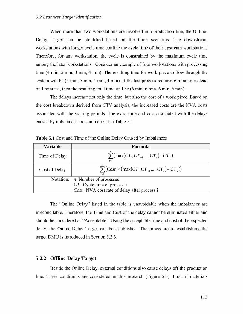
5.2 Leanness Target Identification
When more than two workstations are involved in a production line, the Online-
Delay Target can be identified based on the three scenarios. The downstream
workstations with longer cycle time confine the cycle time of their upstream workstations.
Therefore, for any workstation, the cycle is constrained by the maximum cycle time
among the later workstations. Consider an example of four workstations with processing
time (4 min, 5 min, 3 min, 4 min). The resulting time for work piece to flow through the
system will be (5 min, 5 min, 4 min, 4 min). If the last process requires 6 minutes instead
of 4 minutes, then the resulting total time will be (6 min, 6 min, 6 min, 6 min).
The delays increase not only the time, but also the cost of a work piece. Based on
the cost breakdown derived from CTV analysis, the increased costs are the NVA costs
associated with the waiting periods. The extra time and cost associated with the delays
caused by imbalances are summarized in Table 5.1.
Table 5.1 Cost and Time of the Online Delay Caused by Imbalances
Variable Formula
Time of Delay ( )( )∑=
+ −n
iinii CTCTCTCT
11,...,,max
Cost of Delay ( )( )( )∑=
+ −×n
iiniii CTCTCTCTCost
11,...,,max
Notation: n: Number of processes CTi: Cycle time of process i Costi: NVA cost rate of delay after process i
The “Online Delay” listed in the table is unavoidable when the imbalances are
irreconcilable. Therefore, the Time and Cost of the delay cannot be eliminated either and
should be considered as “Acceptable.” Using the acceptable time and cost of the expected
delay, the Online-Delay Target can be established. The procedure of establishing the
target DMU is introduced in Section 5.2.3.
5.2.2 Offline-Delay Target
Beside the Online Delay, external conditions also cause delays off the production
line. Three conditions are considered in this research (Figure 5.3). First, if materials
113
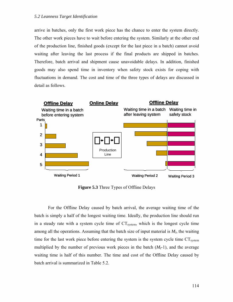
5.2 Leanness Target Identification
arrive in batches, only the first work piece has the chance to enter the system directly.
The other work pieces have to wait before entering the system. Similarly at the other end
of the production line, finished goods (except for the last piece in a batch) cannot avoid
waiting after leaving the last process if the final products are shipped in batches.
Therefore, batch arrival and shipment cause unavoidable delays. In addition, finished
goods may also spend time in inventory when safety stock exists for coping with
fluctuations in demand. The cost and time of the three types of delays are discussed in
detail as follows.
Offline DelayOffline Delay Offline DelayOffline DelayOnline DelayOnline DelayWaiting time in a batchbefore entering system
Waiting time in a batchafter leaving system
Waiting time insafety stock
1
2
3
4
5
Parts
Waiting Period 1 Waiting Period 2 Waiting Period 3
ProductionLine
Offline DelayOffline Delay Offline DelayOffline DelayOnline DelayOnline DelayWaiting time in a batchbefore entering system
Waiting time in a batchafter leaving system
Waiting time insafety stock
1
2
3
4
5
Parts
Waiting Period 1 Waiting Period 2 Waiting Period 3
ProductionLine
Figure 5.3 Three Types of Offline Delays
For the Offline Delay caused by batch arrival, the average waiting time of the
batch is simply a half of the longest waiting time. Ideally, the production line should run
in a steady rate with a system cycle time of CTsystem, which is the longest cycle time
among all the operations. Assuming that the batch size of input material is MI, the waiting
time for the last work piece before entering the system is the system cycle time CTsystem
multiplied by the number of previous work pieces in the batch (MI-1), and the average
waiting time is half of this number. The time and cost of the Offline Delay caused by
batch arrival is summarized in Table 5.2.
114
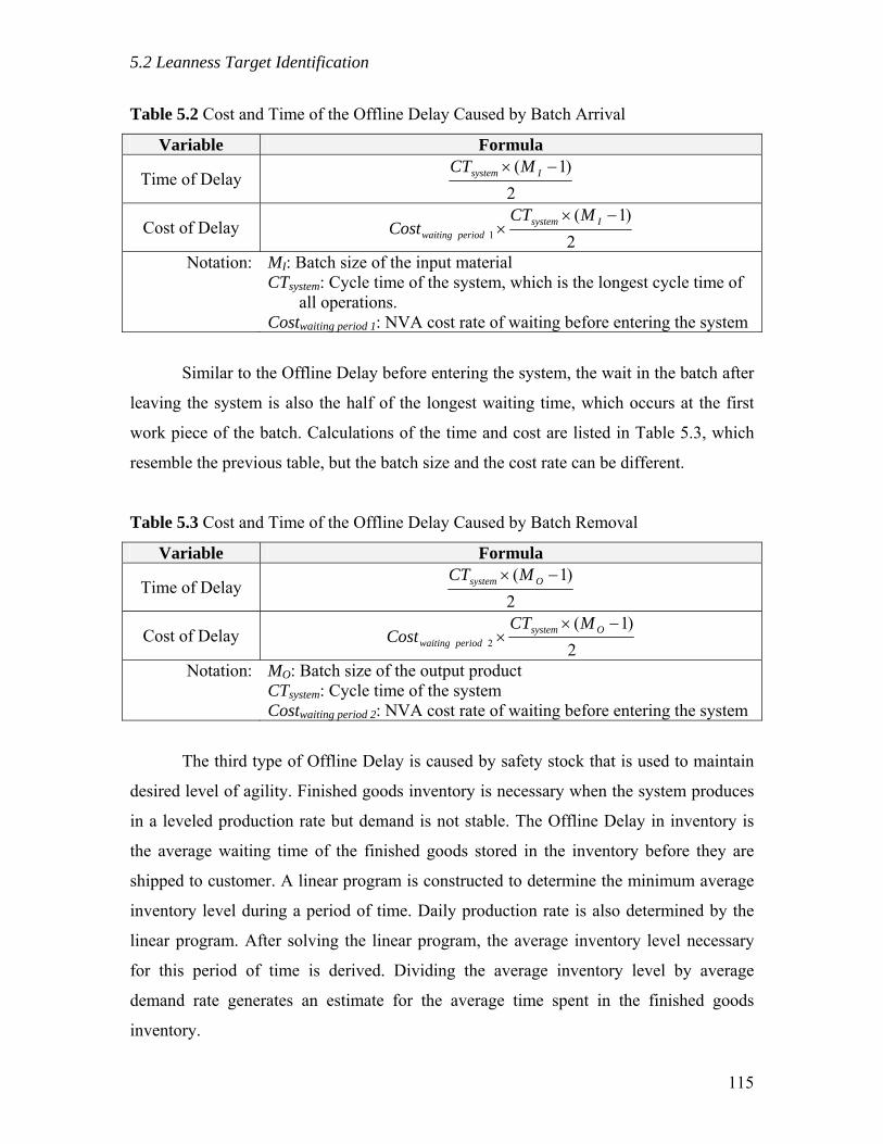
5.2 Leanness Target Identification
Table 5.2 Cost and Time of the Offline Delay Caused by Batch Arrival
Variable Formula
Time of Delay 2
)1( −× Isystem MCT
Cost of Delay 2
)1(1
−×× Isystem
periodwaiting
MCTCost
Notation: MI: Batch size of the input material CTsystem: Cycle time of the system, which is the longest cycle time of
all operations. Costwaiting period 1: NVA cost rate of waiting before entering the system
Similar to the Offline Delay before entering the system, the wait in the batch after
leaving the system is also the half of the longest waiting time, which occurs at the first
work piece of the batch. Calculations of the time and cost are listed in Table 5.3, which
resemble the previous table, but the batch size and the cost rate can be different.
Table 5.3 Cost and Time of the Offline Delay Caused by Batch Removal
Variable Formula
Time of Delay 2
)1( −× Osystem MCT
Cost of Delay 2
)1(2
−×× Osystem
periodwaiting
MCTCost
Notation: MO: Batch size of the output product CTsystem: Cycle time of the system Costwaiting period 2: NVA cost rate of waiting before entering the system
The third type of Offline Delay is caused by safety stock that is used to maintain
desired level of agility. Finished goods inventory is necessary when the system produces
in a leveled production rate but demand is not stable. The Offline Delay in inventory is
the average waiting time of the finished goods stored in the inventory before they are
shipped to customer. A linear program is constructed to determine the minimum average
inventory level during a period of time. Daily production rate is also determined by the
linear program. After solving the linear program, the average inventory level necessary
for this period of time is derived. Dividing the average inventory level by average
demand rate generates an estimate for the average time spent in the finished goods
inventory.
115

5.2 Leanness Target Identification
The linear program and the calculation of the acceptable Offline Delay are
discussed as follows.
Linear Program for Minimum Average Inventory
Min. k
Iz
k
ii∑
== 1 (34)
S.T. P + Ii-1 = Di + Ii for i= 1 to k (35)
where, z is the minimum average inventory level;
Ii is the daily inventory level;
k is the number of days being considered for a leveled production rate;
P is the daily production rate;
Di is the daily demand.
In the program, the number “k” is the time span being considered for a fixed
production rate. For a certain level of demand fluctuation, the choice of “k” determines
the inventory level and the production rate. For example, the production rate can be
chosen to be changed daily to meet the demand without inventory, or it can be changes
every week with an inventory level to satisfy the maximum demand of the week. If the
demand is not stable, a smaller k makes the production rate change frequently, but lower
safety stock level is needed. On the contrary, a larger k leads to stable production rate
over longer period of time, but higher inventory level is necessary to meet the changing
demand. There, the number k determines the agility level chosen by the decision maker.
If the daily production rate exceeds the capacity of the system, the demand can be met by
working overtime or outsourcing for extra capacity. Or the company may need to give up
on the extra portion of the demand if it cannot be back logged.
With the results of the linear program, the Offline Delay caused by finished goods
inventory can be calculated as shown in Table 5.4.
116
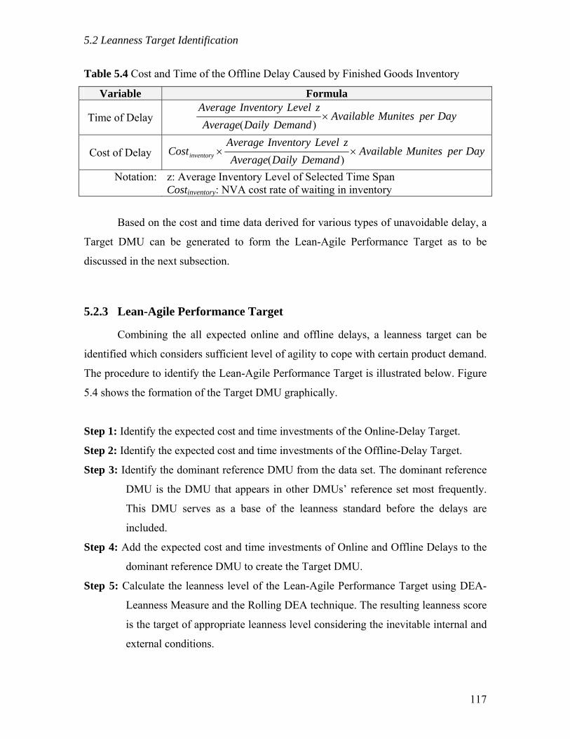
5.2 Leanness Target Identification
Table 5.4 Cost and Time of the Offline Delay Caused by Finished Goods Inventory
Variable Formula
Time of Delay DayperMunitesAvailableDemandDailyAverage
zLevelInventoryAverage×
)(
Cost of Delay DayperMunitesAvailableDemandDailyAverage
zLevelInventoryAverageCostinventory ××
)(Notation: z: Average Inventory Level of Selected Time Span
Costinventory: NVA cost rate of waiting in inventory
Based on the cost and time data derived for various types of unavoidable delay, a
Target DMU can be generated to form the Lean-Agile Performance Target as to be
discussed in the next subsection.
5.2.3 Lean-Agile Performance Target
Combining the all expected online and offline delays, a leanness target can be
identified which considers sufficient level of agility to cope with certain product demand.
The procedure to identify the Lean-Agile Performance Target is illustrated below. Figure
5.4 shows the formation of the Target DMU graphically.
Step 1: Identify the expected cost and time investments of the Online-Delay Target.
Step 2: Identify the expected cost and time investments of the Offline-Delay Target.
Step 3: Identify the dominant reference DMU from the data set. The dominant reference
DMU is the DMU that appears in other DMUs’ reference set most frequently.
This DMU serves as a base of the leanness standard before the delays are
included.
Step 4: Add the expected cost and time investments of Online and Offline Delays to the
dominant reference DMU to create the Target DMU.
Step 5: Calculate the leanness level of the Lean-Agile Performance Target using DEA-
Leanness Measure and the Rolling DEA technique. The resulting leanness score
is the target of appropriate leanness level considering the inevitable internal and
external conditions.
117
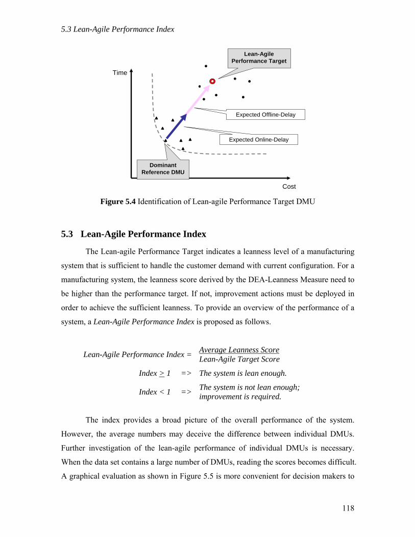
5.3 Lean-Agile Performance Index
Cost
Time
Expected Online-Delay
LeanLean--Agile Agile Performance TargetPerformance Target
Dominant Dominant Reference DMUReference DMU
Expected Offline-Delay
Figure 5.4 Identification of Lean-agile Performance Target DMU
5.3 Lean-Agile Performance Index
The Lean-agile Performance Target indicates a leanness level of a manufacturing
system that is sufficient to handle the customer demand with current configuration. For a
manufacturing system, the leanness score derived by the DEA-Leanness Measure need to
be higher than the performance target. If not, improvement actions must be deployed in
order to achieve the sufficient leanness. To provide an overview of the performance of a
system, a Lean-Agile Performance Index is proposed as follows.
Lean-Agile Performance Index = Average Leanness Score Lean-Agile Target Score
Index > 1 => The system is lean enough.
Index < 1 => The system is not lean enough; improvement is required.
The index provides a broad picture of the overall performance of the system.
However, the average numbers may deceive the difference between individual DMUs.
Further investigation of the lean-agile performance of individual DMUs is necessary.
When the data set contains a large number of DMUs, reading the scores becomes difficult.
A graphical evaluation as shown in Figure 5.5 is more convenient for decision makers to
118
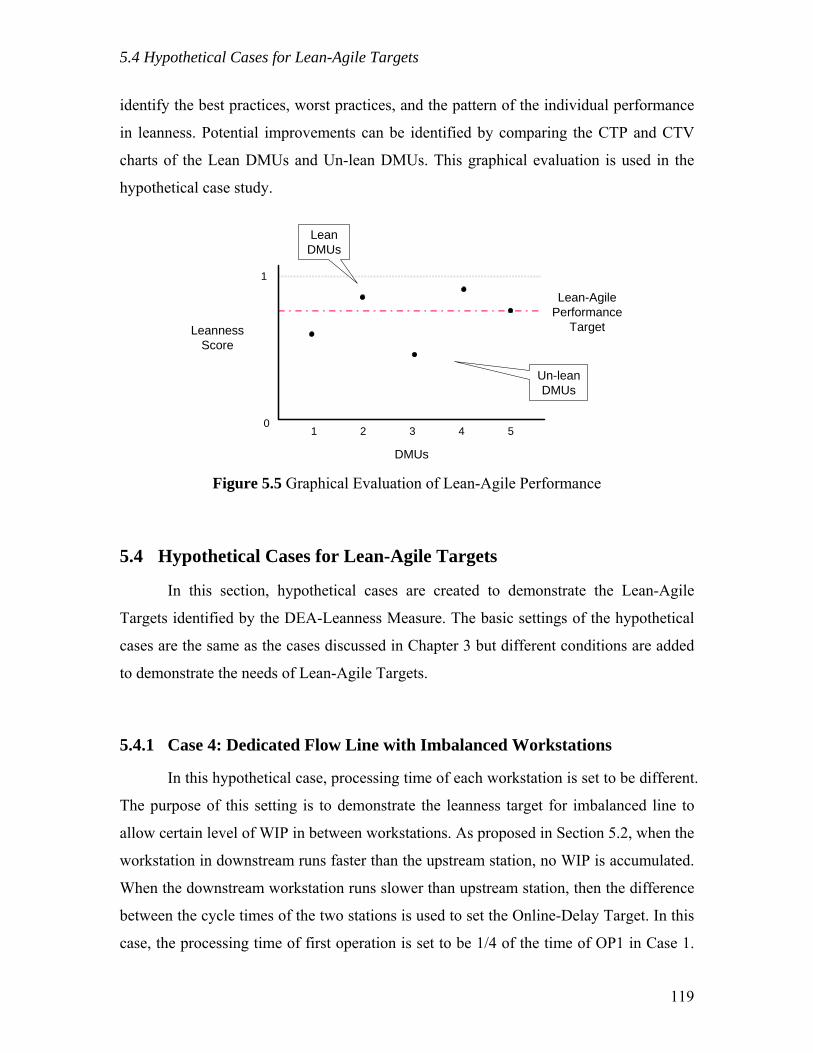
5.4 Hypothetical Cases for Lean-Agile Targets
identify the best practices, worst practices, and the pattern of the individual performance
in leanness. Potential improvements can be identified by comparing the CTP and CTV
charts of the Lean DMUs and Un-lean DMUs. This graphical evaluation is used in the
hypothetical case study.
DMUs
1 2 3 4 5
LeannessScore
0
1
Lean-AgilePerformance
Target
Un-lean DMUs
Lean DMUs
Figure 5.5 Graphical Evaluation of Lean-Agile Performance
5.4 Hypothetical Cases for Lean-Agile Targets
In this section, hypothetical cases are created to demonstrate the Lean-Agile
Targets identified by the DEA-Leanness Measure. The basic settings of the hypothetical
cases are the same as the cases discussed in Chapter 3 but different conditions are added
to demonstrate the needs of Lean-Agile Targets.
5.4.1 Case 4: Dedicated Flow Line with Imbalanced Workstations
In this hypothetical case, processing time of each workstation is set to be different.
The purpose of this setting is to demonstrate the leanness target for imbalanced line to
allow certain level of WIP in between workstations. As proposed in Section 5.2, when the
workstation in downstream runs faster than the upstream station, no WIP is accumulated.
When the downstream workstation runs slower than upstream station, then the difference
between the cycle times of the two stations is used to set the Online-Delay Target. In this
case, the processing time of first operation is set to be 1/4 of the time of OP1 in Case 1.
119
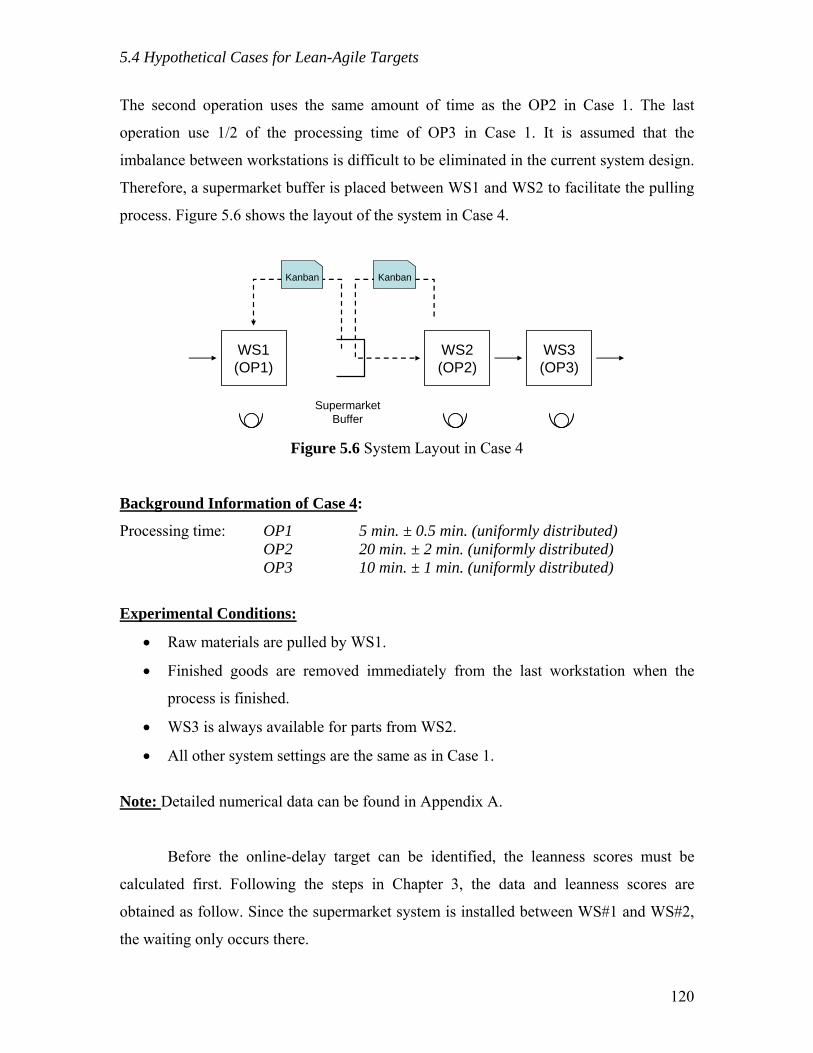
5.4 Hypothetical Cases for Lean-Agile Targets
The second operation uses the same amount of time as the OP2 in Case 1. The last
operation use 1/2 of the processing time of OP3 in Case 1. It is assumed that the
imbalance between workstations is difficult to be eliminated in the current system design.
Therefore, a supermarket buffer is placed between WS1 and WS2 to facilitate the pulling
process. Figure 5.6 shows the layout of the system in Case 4.
WS1(OP1)
WS2(OP2)
WS3(OP3)
SupermarketBuffer
KanbanKanban
Figure 5.6 System Layout in Case 4
Background Information of Case 4:
Processing time: OP1 5 min. ± 0.5 min. (uniformly distributed) OP2 20 min. ± 2 min. (uniformly distributed) OP3 10 min. ± 1 min. (uniformly distributed)
Experimental Conditions:
• Raw materials are pulled by WS1.
• Finished goods are removed immediately from the last workstation when the
process is finished.
• WS3 is always available for parts from WS2.
• All other system settings are the same as in Case 1.
Note: Detailed numerical data can be found in Appendix A.
Before the online-delay target can be identified, the leanness scores must be
calculated first. Following the steps in Chapter 3, the data and leanness scores are
obtained as follow. Since the supermarket system is installed between WS#1 and WS#2,
the waiting only occurs there.
120
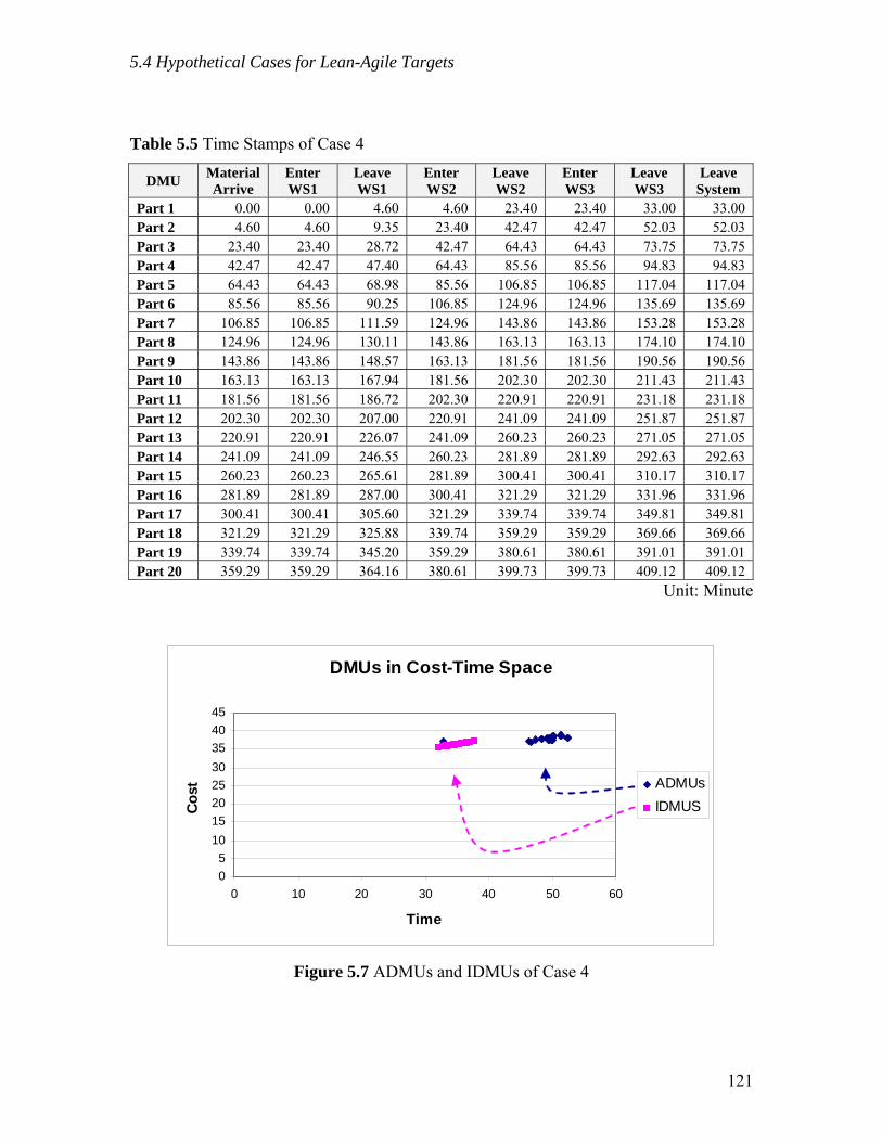
5.4 Hypothetical Cases for Lean-Agile Targets
Table 5.5 Time Stamps of Case 4
DMU Material Arrive
Enter WS1
Leave WS1
Enter WS2
Leave WS2
Enter WS3
Leave WS3
Leave System
Part 1 0.00 0.00 4.60 4.60 23.40 23.40 33.00 33.00 Part 2 4.60 4.60 9.35 23.40 42.47 42.47 52.03 52.03 Part 3 23.40 23.40 28.72 42.47 64.43 64.43 73.75 73.75 Part 4 42.47 42.47 47.40 64.43 85.56 85.56 94.83 94.83 Part 5 64.43 64.43 68.98 85.56 106.85 106.85 117.04 117.04 Part 6 85.56 85.56 90.25 106.85 124.96 124.96 135.69 135.69 Part 7 106.85 106.85 111.59 124.96 143.86 143.86 153.28 153.28 Part 8 124.96 124.96 130.11 143.86 163.13 163.13 174.10 174.10 Part 9 143.86 143.86 148.57 163.13 181.56 181.56 190.56 190.56 Part 10 163.13 163.13 167.94 181.56 202.30 202.30 211.43 211.43 Part 11 181.56 181.56 186.72 202.30 220.91 220.91 231.18 231.18 Part 12 202.30 202.30 207.00 220.91 241.09 241.09 251.87 251.87 Part 13 220.91 220.91 226.07 241.09 260.23 260.23 271.05 271.05 Part 14 241.09 241.09 246.55 260.23 281.89 281.89 292.63 292.63 Part 15 260.23 260.23 265.61 281.89 300.41 300.41 310.17 310.17 Part 16 281.89 281.89 287.00 300.41 321.29 321.29 331.96 331.96 Part 17 300.41 300.41 305.60 321.29 339.74 339.74 349.81 349.81 Part 18 321.29 321.29 325.88 339.74 359.29 359.29 369.66 369.66 Part 19 339.74 339.74 345.20 359.29 380.61 380.61 391.01 391.01 Part 20 359.29 359.29 364.16 380.61 399.73 399.73 409.12 409.12
Unit: Minute
DMUs in Cost-Time Space
05
1015202530354045
0 10 20 30 40 50 60
Time
Cost
ADMUsIDMUS
Figure 5.7 ADMUs and IDMUs of Case 4
121
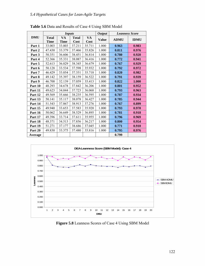
5.4 Hypothetical Cases for Lean-Agile Targets
Table 5.6 Data and Results of Case 4 Using SBM Model
Inputs Output Leanness Score DMU Total
Time VA
Time Total Cost
VA Cost Value ADMU IDMU
Part 1 33.003 33.003 37.211 35.711 1.000 0.963 0.983 Part 2 47.430 33.379 37.466 35.826 1.000 0.811 0.976 Part 3 50.351 36.606 38.451 36.814 1.000 0.780 0.920 Part 4 52.366 35.331 38.087 36.416 1.000 0.772 0.941 Part 5 52.613 36.029 38.345 36.679 1.000 0.767 0.929 Part 6 50.128 33.534 37.598 35.932 1.000 0.792 0.972 Part 7 46.429 33.054 37.351 35.718 1.000 0.820 0.982 Part 8 49.142 35.397 38.159 36.522 1.000 0.791 0.939 Part 9 46.700 32.139 37.059 35.413 1.000 0.822 1.000 Part 10 48.293 34.678 37.842 36.206 1.000 0.801 0.952 Part 11 49.623 34.044 37.723 36.068 1.000 0.793 0.963 Part 12 49.569 35.666 38.235 36.595 1.000 0.787 0.934 Part 13 50.141 35.117 38.078 36.427 1.000 0.785 0.944 Part 14 51.543 37.867 38.913 37.276 1.000 0.767 0.899 Part 15 49.940 33.653 37.583 35.920 1.000 0.793 0.970 Part 16 50.062 36.649 38.529 36.895 1.000 0.781 0.918 Part 17 49.396 33.714 37.611 35.955 1.000 0.796 0.969 Part 18 48.371 34.513 37.856 36.217 1.000 0.800 0.954 Part 19 51.271 37.177 38.686 37.045 1.000 0.771 0.910 Part 20 49.830 33.375 37.480 35.816 1.000 0.795 0.976 Average 0.799
DEA-Leanness Score (SBM Model): Case 4
0.000
0.100
0.200
0.300
0.400
0.500
0.600
0.700
0.800
0.900
1.000
1 2 3 4 5 6 7 8 9 10 11 12 13 14 15 16 17 18 19 20
DMU
Lean
nes
SBM ADMUSBM IDMU
Figure 5.8 Leanness Scores of Case 4 Using SBM Model
122
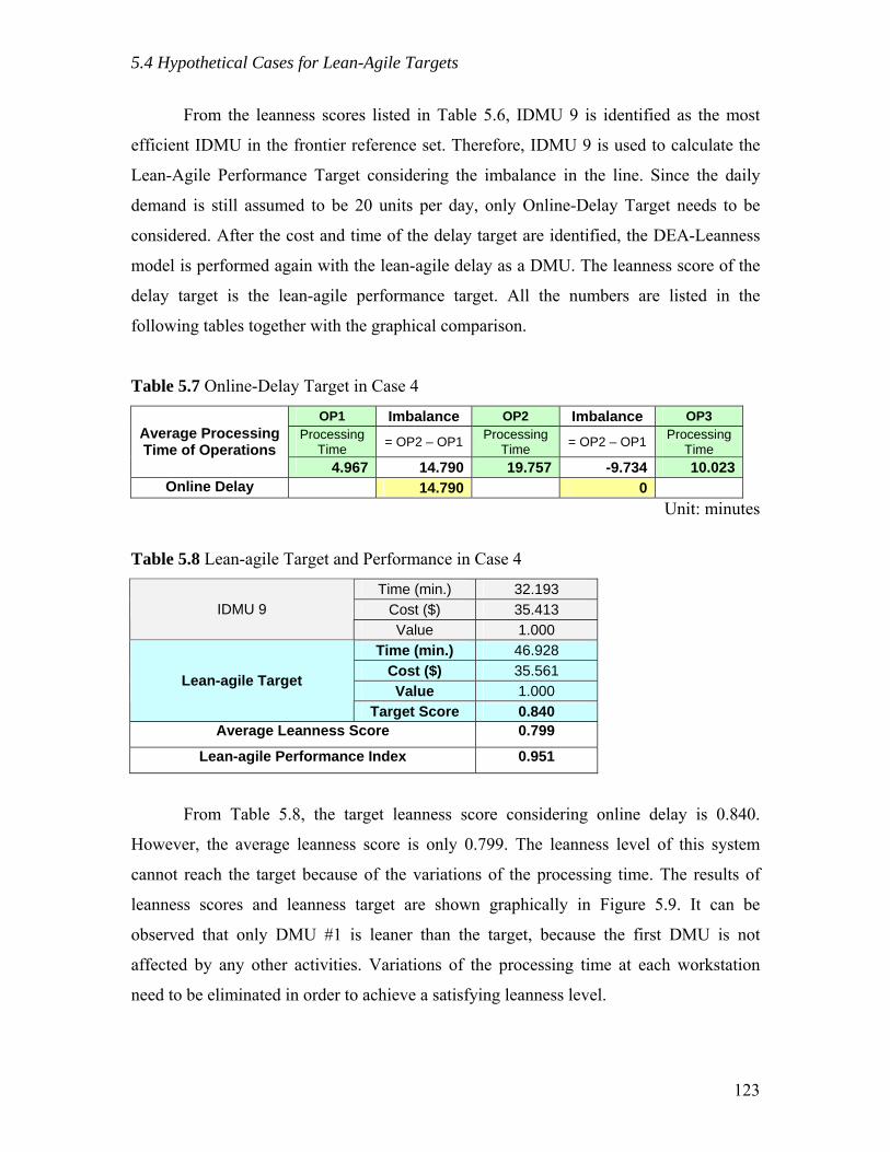
5.4 Hypothetical Cases for Lean-Agile Targets
From the leanness scores listed in Table 5.6, IDMU 9 is identified as the most
efficient IDMU in the frontier reference set. Therefore, IDMU 9 is used to calculate the
Lean-Agile Performance Target considering the imbalance in the line. Since the daily
demand is still assumed to be 20 units per day, only Online-Delay Target needs to be
considered. After the cost and time of the delay target are identified, the DEA-Leanness
model is performed again with the lean-agile delay as a DMU. The leanness score of the
delay target is the lean-agile performance target. All the numbers are listed in the
following tables together with the graphical comparison.
Table 5.7 Online-Delay Target in Case 4
OP1 Imbalance OP2 Imbalance OP3 Processing
Time = OP2 – OP1 Processing Time = OP2 – OP1 Processing
Time Average Processing Time of Operations
4.967 14.790 19.757 -9.734 10.023Online Delay 14.790 0
Unit: minutes
Table 5.8 Lean-agile Target and Performance in Case 4
Time (min.) 32.193 Cost ($) 35.413 IDMU 9 Value 1.000
Time (min.) 46.928 Cost ($) 35.561 Value 1.000
Lean-agile Target
Target Score 0.840 Average Leanness Score 0.799
Lean-agile Performance Index 0.951
From Table 5.8, the target leanness score considering online delay is 0.840.
However, the average leanness score is only 0.799. The leanness level of this system
cannot reach the target because of the variations of the processing time. The results of
leanness scores and leanness target are shown graphically in Figure 5.9. It can be
observed that only DMU #1 is leaner than the target, because the first DMU is not
affected by any other activities. Variations of the processing time at each workstation
need to be eliminated in order to achieve a satisfying leanness level.
123

5.4 Hypothetical Cases for Lean-Agile Targets
DEA-Leanness Score (SBM Model): Case 4
0.000
0.100
0.200
0.300
0.400
0.500
0.600
0.700
0.800
0.900
1.000
1 2 3 4 5 6 7 8 9 10 11 12 13 14 15 16 17 18 19 20
DMU
Lean
nes SBM ADMU
SBM IDMULeanness Target
Figure 5.9 Lean-Agile Target and Performance in Case 4
5.4.2 Case 5: Dedicated Flow Line with Fluctuating Demand
In this hypothetical case, fluctuation in demand quantity is introduced to
demonstrate the identification of Offline-Delay Target. The settings of this case are
created based on Case 1, but five days of production is considered. The detailed settings
of this case are listed below. Overtime will be used when the daily demand cannot be met
by the regular working time.
Background Information of Case 5:
Weekly Schedule: Day 1 20 units of Product A Day 2 15 units of Product A Day 3 30 units of Product A Day 4 10 units of Product A Day 5 25 units of Product A
Regular Working Time: 8 hours/day = 480 minutes/day
Daily Production Rate: 20 units/day
Takt Time: 24 minutes/unit
Processing time: OP1 20 min. ± 2 min. (uniformly distributed) OP2 20 min. ± 2 min. (uniformly distributed) OP3 20 min. ± 2 min. (uniformly distributed)
124
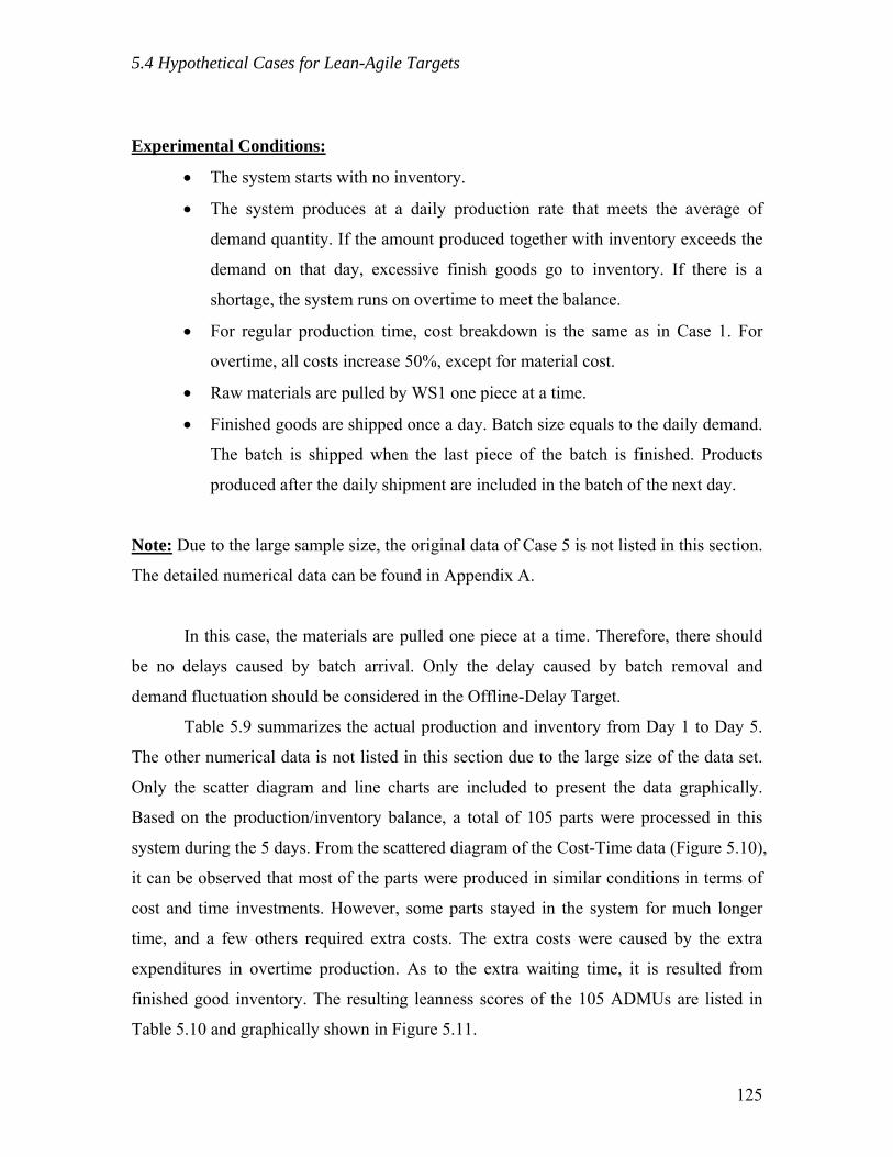
5.4 Hypothetical Cases for Lean-Agile Targets
Experimental Conditions:
• The system starts with no inventory.
• The system produces at a daily production rate that meets the average of
demand quantity. If the amount produced together with inventory exceeds the
demand on that day, excessive finish goods go to inventory. If there is a
shortage, the system runs on overtime to meet the balance.
• For regular production time, cost breakdown is the same as in Case 1. For
overtime, all costs increase 50%, except for material cost.
• Raw materials are pulled by WS1 one piece at a time.
• Finished goods are shipped once a day. Batch size equals to the daily demand.
The batch is shipped when the last piece of the batch is finished. Products
produced after the daily shipment are included in the batch of the next day.
Note: Due to the large sample size, the original data of Case 5 is not listed in this section.
The detailed numerical data can be found in Appendix A.
In this case, the materials are pulled one piece at a time. Therefore, there should
be no delays caused by batch arrival. Only the delay caused by batch removal and
demand fluctuation should be considered in the Offline-Delay Target.
Table 5.9 summarizes the actual production and inventory from Day 1 to Day 5.
The other numerical data is not listed in this section due to the large size of the data set.
Only the scatter diagram and line charts are included to present the data graphically.
Based on the production/inventory balance, a total of 105 parts were processed in this
system during the 5 days. From the scattered diagram of the Cost-Time data (Figure 5.10),
it can be observed that most of the parts were produced in similar conditions in terms of
cost and time investments. However, some parts stayed in the system for much longer
time, and a few others required extra costs. The extra costs were caused by the extra
expenditures in overtime production. As to the extra waiting time, it is resulted from
finished good inventory. The resulting leanness scores of the 105 ADMUs are listed in
Table 5.10 and graphically shown in Figure 5.11.
125

5.4 Hypothetical Cases for Lean-Agile Targets
Table 5.9 Actual Demand, Inventory and Overtime of Case 5
Daily Demand Inventory Unit Produced in Overtime Initial 0 Day 1 20 0 0 Day 2 15 5 0 Day 3 30 0 5 Day 4 10 10 0 Day 5 25 5 0
Daily Production: 20 units
Day 1 to Day 5 in Case 5
0.00
10.00
20.00
30.00
40.00
50.00
60.00
70.00
80.00
0.00 100.00 200.00 300.00 400.00 500.00 600.00 700.00 800.00
Time (min.)
Cos
t ($)
ADMU
IDMU
Figure 5.10 ADMUs and IDMUs in Case 5
Table 5.10 Summary of DEA-Leanness Measurement of Case 5
Average Leanness Score of ADMUs: 0.570
DMUs on Frontier IDMU 1 (referred frequency: 5/105)
IDMU 13 (referred frequency: 100/105)
126

5.4 Hypothetical Cases for Lean-Agile Targets
Leanness Score of Case 5
0
0.1
0.2
0.3
0.4
0.5
0.6
0.7
0.8
0.9
1
1 5 9 13 17 21 25 29 33 37 41 45 49 53 57 61 65 69 73 77 81 85 89 93 97 101 105
ADMU
Lean
ness
Figure 5.11 Leanness Scores of Case 5
From Table 5.10, IDMU 13 is clearly the dominant DMU on the frontier.
Therefore, the Offline-Delay Target DMU can be constructed using the Cost/Time/Value
data of IDMU 13. First, the Offline Delay caused by batch removal is calculated. The
average cycle time is 20 minutes. Since the demand changes daily, an average of the five
days’ data is calculated.
Table 5.11 Offline Delay of Case 5
Variable Offline Delay Caused by Batch Removal
Time of Delay Average ( 2
)1( −× Osystem MCT) = 190 minutes
Cost of Delay 2
)1(2
−×× Osystem
periodwaiting
MCTCost = $1.90
The next step is to calculate the minimum average inventory level with a constant
production rate. A mathematical program is developed to determine the minimum value.
127
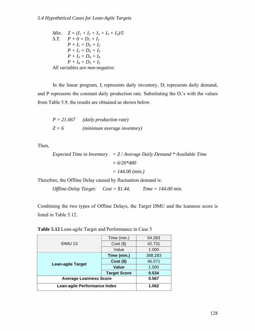
5.4 Hypothetical Cases for Lean-Agile Targets
Min. Z = (I1 + I2 + I3 + I4 + I5)/5 S.T. P + 0 = D1 + I1 P + I1 = D2 + I2 P + I2 = D3 + I3 P + I3 = D4 + I4 P + I4 = D5 + I5 All variables are non-negative.
In the linear program, Ii represents daily inventory, Di represents daily demand,
and P represents the constant daily production rate. Substituting the Di’s with the values
from Table 5.9, the results are obtained as shown below.
P = 21.667 (daily production rate)
Z = 6 (minimum average inventory)
Then,
Expected Time in Inventory = Z / Average Daily Demand * Available Time
= 6/20*480
= 144.00 (min.)
Therefore, the Offline Delay caused by fluctuation demand is:
Offline-Delay Target: Cost = $1.44, Time = 144.00 min.
Combining the two types of Offline Delays, the Target DMU and the leanness score is
listed in Table 5.12.
Table 5.12 Lean-agile Target and Performance in Case 5
Time (min.) 54.283 Cost ($) 42.731 IDMU 13 Value 1.000
Time (min.) 388.283 Cost ($) 46.071 Value 1.000
Lean-agile Target
Target Score 0.534 Average Leanness Score 0.567
Lean-agile Performance Index 1.062
128
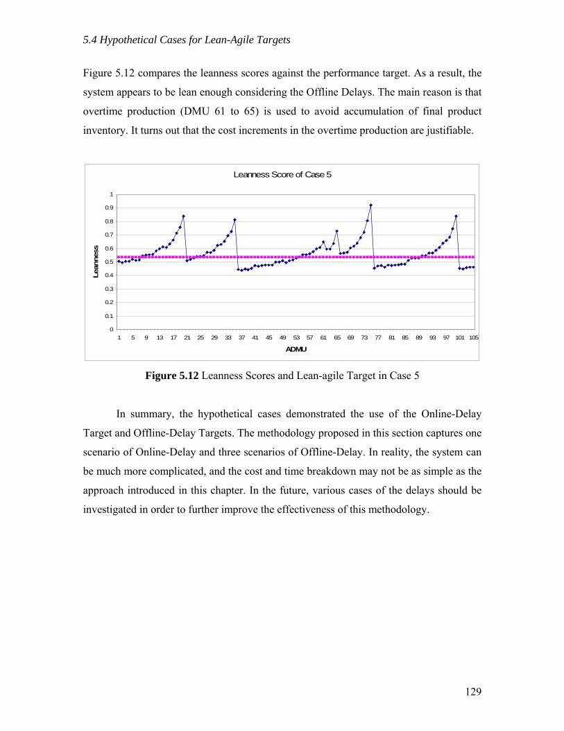
5.4 Hypothetical Cases for Lean-Agile Targets
Figure 5.12 compares the leanness scores against the performance target. As a result, the
system appears to be lean enough considering the Offline Delays. The main reason is that
overtime production (DMU 61 to 65) is used to avoid accumulation of final product
inventory. It turns out that the cost increments in the overtime production are justifiable.
Leanness Score of Case 5
0
0.1
0.2
0.3
0.4
0.5
0.6
0.7
0.8
0.9
1
1 5 9 13 17 21 25 29 33 37 41 45 49 53 57 61 65 69 73 77 81 85 89 93 97 101 105
ADMU
Lean
ness
Figure 5.12 Leanness Scores and Lean-agile Target in Case 5
In summary, the hypothetical cases demonstrated the use of the Online-Delay
Target and Offline-Delay Targets. The methodology proposed in this section captures one
scenario of Online-Delay and three scenarios of Offline-Delay. In reality, the system can
be much more complicated, and the cost and time breakdown may not be as simple as the
approach introduced in this chapter. In the future, various cases of the delays should be
investigated in order to further improve the effectiveness of this methodology.
129
6.1 A Web-based Kanban System
Chapter 6 Software Implementation of DEA-Leanness
Measure
The proposed methodology of DEA-Leanness Measure evaluates the leanness
level and lean-agile performance of manufacturing systems by comparing the production
activities of every work piece. To evaluate the leanness level, cost and time investments
of all activities on the value stream need to be recorded in detail, and the VA investments
need to be distinguished from the NVA investments. In order to handle the huge amount
of data, two computer programs have been developed to realize this methodology. First, a
Web-based Kanban System is developed to collect the time stamps of production
activities. This data can be transformed into VA and NVA intervals, and then, Cost and
Value data can be added to generate ADMUs and IDMUs for the DEA-Leanness
Measure. Another software program developed in this research is an Excel-based DEA
Solver that solves the SBM model and provides leanness scores. The CTV Charts of
DMUs are also generated for the users to identify wastes from the production processes.
With the two software programs, the cumbersome processes of data collection and
analysis can be carried out by computers. This chapter discusses the two software
programs starting with the Web-Kanban System.
6.1 A Web-based Kanban System
As introduced in the previous chapters, various approaches, such as Rolling DEA,
have been developed to address potential barriers of applying the DEA-Leanness
Measure. However, the methodologies and mathematical models introduced previously
have not addressed the potential difficulty on data collection for the leanness measure. If
a delicate computer system, such as Enterprise Resources Planning (ERP) system, is
already in place and can provide detailed information on Time, Cost and Value required
by the model, the data collection process should not a problem. Nevertheless, the
investment on installing an ERP system is known to be enormous and many small and
130

6.1 A Web-based Kanban System
medium sized companies cannot afford ERP. In that situation, the Cost and Value data
can be identified later when the processes are finished. However, time stamps of each
activity need to be recorded while it is progressing via various steps. The Time data can
be collected manually by operators or a dedicated observer on site. However, when the
products flow through the system with a relatively fast pace, manual timing would be a
burden for the online operators. On the other hand, timing each production activity by an
observer may be difficult if multiple products are processed in a production line by
different workstations. The observer will not be able to keep detailed track of each
product. Consequently, a computerized system that keeps the timing records of all
production activities is in need. A Web-based Kanban System developed in this research
is to facilitate the automated data collection for DEA-Leanness Measure.
6.1.1 Background of Web-Kanban System Development
Kanban is known to be one of the most important tools of the Toyota Production
System (TPS). The Japanese word, Kanban, means a card with visual information that
conducts the information flows in the TPS (Monden, 1998). Because of the simplicity
and effectiveness of the Kanban system in shop floor control, it has become one of the
most powerful tools for implementing lean concepts. However, lacking of the capability
to track and monitor physical Kanbans is the weakness of the traditional Kanban system.
In a conventional Kanban system, the Kanbans are not tracked, and the performance of
executing a task triggered by a Kanban is not monitored or recorded. A computerized
Kanban system can effectively address this weakness.
Among various programming environments, web-based programming owns
several features that facilitate the computerized Kanban system. A web-based Kanban
system can be simple, effective and easy to use. The reasons to integrate Kanban systems
with web-based technology are listed as follows.
1) Standard User Interface: Web browser has become a standard feature of every
operating system in computers. Various web browsers (e.g., Explorer by Microsoft,
Firefox by Netscape, etc.) have been developed, and all of them interpret the standard
131

6.1 A Web-based Kanban System
HyperText Markup Language (HTML) in the same way even in different operating
systems, such as Windows, Apple, or UNIX. Even some handheld devices, such as
Personal Digital Assistant (PDA) and cell phone, can browse web pages. Therefore,
the web browsers provide a standardized user interface regardless the type of
computer system. The cross-platform compatibility makes web-based programs
accessible to any users connected to the server.
2) Easy Connections: In the past decade, web connection has become readily available
in most of the working environments. Web services can be accessed by computers or
handheld devices through wired or wireless network. Implementing a web-based
Kanban system does not require additional investment on hardware if Internet or
Intranet service is available at workstations in the shop floor.
3) Improved Web-based Program Capability: The computational capacity of web-
based program has been improved dramatically in the past decade. Traditional HTML
files provide only static contents to the users. In contrast to the static web pages, the
newly developed web-based programming environment supports “dynamic” web
pages which facilitates interactive web browsing and computational capabilities.
Together with web-based databases, the servers can provide functional web pages for
various purposes. For manufacturing systems, the functions, such as Real-time
tracking, Performance measurement, Interactive input/output, Dynamic display, etc.,
can all be achieved by web-based programs now.
Based on the aforementioned features, developing a Kanban system using web-
based technology is a solution to address the weakness of the TPS tool. Following
improvements on functionality are expected when upgrading a physical Kanban system
to a web-based system.
1) Real-time Kanban Tracking: Improved capability on Kanban tracking and
monitoring can be achieved by web-based services. The time stamps of all
movements of a Kanban can be recorded in real time for performance analysis.
2) Higher Capacity of Information Flow: More information can be embedded and
delivered by a web-based Kanban than that of a physical Kanban. Not only the size of
132
6.1 A Web-based Kanban System
information carried by the Kanbans can be increased, the web-based Kanban can also
deliver different formats of information, such as electronic CAD/CAM files, audio
streams, video clips, etc., which dramatically improves the capability of conducting
the information flow. Furthermore, other online information can always be linked
from a web-based Kanban, which eliminates the limit of the size of information a
Kanban can carry.
3) Wide Range of Application: The web-based system can be applied to different
settings, including Pull Production System, Push Production System, Project-
Oriented Production, Project Management, Documentation System, etc.
4) Performance Monitoring: Most importantly for this research, the web-based Kanban
system can evaluate the performance of the system in real time. Since all Kanbans are
dispatched and monitored by the web server, the data of cost and time can be
generated accordingly. Therefore, the leanness measurement can be implemented
through the web-based Kanban system. Functionality extensions, such as integration
with sensors, barcode and RFID systems, are foreseeable to increase the efficiency of
leanness measurement.
With the abovementioned expectations, a Web-Kanban System is established
using server-executed web-based program together with Internet database. In this
research, the Web-Kanban System serves as an implementation of the DEA-Leanness
measure. It can also be a starting point for the construction of a web-based manufacturing
system. Eventually, a Performance-Oriented web-based manufacturing system can be
carried out (Wan and Chen, 2004). Details of the Web-Kanban System are introduced in
the following subsections.
6.1.2 Framework and Functionality of Web-Kanban System
In this research, a web-based program is developed to run a computerized Kanban
system which is capable of collecting time-based performance data for the DEA-
Leanness Measure. In addition to network connections, the Web-Kanban System
developed in this research contains the following components:
133
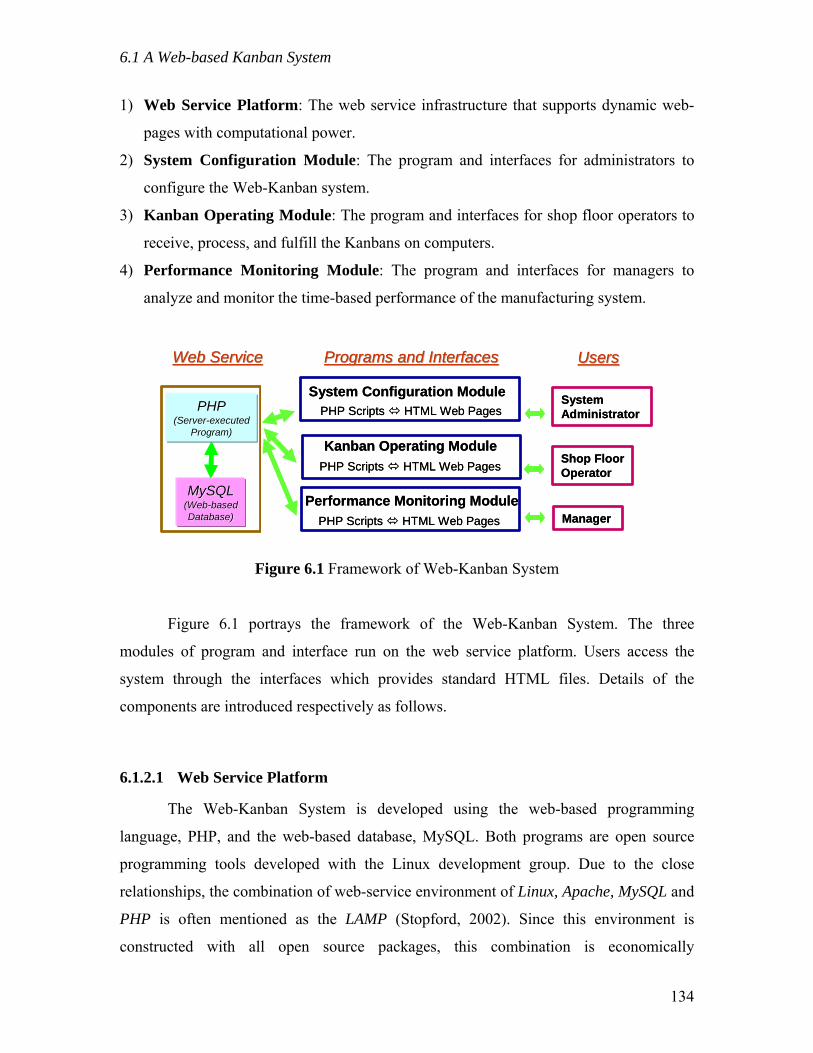
6.1 A Web-based Kanban System
1) Web Service Platform: The web service infrastructure that supports dynamic web-
pages with computational power.
2) System Configuration Module: The program and interfaces for administrators to
configure the Web-Kanban system.
3) Kanban Operating Module: The program and interfaces for shop floor operators to
receive, process, and fulfill the Kanbans on computers.
4) Performance Monitoring Module: The program and interfaces for managers to
analyze and monitor the time-based performance of the manufacturing system.
UsersUsersPrograms and InterfacesPrograms and InterfacesWeb ServiceWeb Service
PHPPHP(Server(Server--executedexecuted
Program)Program)
MySQLMySQL(Web(Web--basedbasedDatabase)Database)
UsersUsersPrograms and InterfacesPrograms and InterfacesWeb ServiceWeb Service
System Configuration Module
Kanban Operating Module
Performance Monitoring Module
PHP Scripts HTML Web Pages
PHP Scripts HTML Web Pages
PHP Scripts HTML Web Pages
SystemAdministrator
Shop FloorOperator
Manager
PHPPHP(Server(Server--executedexecuted
Program)Program)
MySQLMySQL(Web(Web--basedbasedDatabase)Database)
System Configuration Module
Kanban Operating Module
Performance Monitoring Module
PHP Scripts HTML Web Pages
PHP Scripts HTML Web Pages
PHP Scripts HTML Web Pages
SystemAdministrator
Shop FloorOperator
Manager
Figure 6.1 Framework of Web-Kanban System
Figure 6.1 portrays the framework of the Web-Kanban System. The three
modules of program and interface run on the web service platform. Users access the
system through the interfaces which provides standard HTML files. Details of the
components are introduced respectively as follows.
6.1.2.1 Web Service Platform
The Web-Kanban System is developed using the web-based programming
language, PHP, and the web-based database, MySQL. Both programs are open source
programming tools developed with the Linux development group. Due to the close
relationships, the combination of web-service environment of Linux, Apache, MySQL and
PHP is often mentioned as the LAMP (Stopford, 2002). Since this environment is
constructed with all open source packages, this combination is economically
134
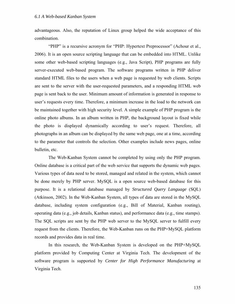
6.1 A Web-based Kanban System
advantageous. Also, the reputation of Linux group helped the wide acceptance of this
combination.
“PHP” is a recursive acronym for “PHP: Hypertext Preprocessor” (Achour et al.,
2006). It is an open source scripting language that can be embedded into HTML. Unlike
some other web-based scripting languages (e.g., Java Script), PHP programs are fully
server-executed web-based program. The software programs written in PHP deliver
standard HTML files to the users when a web page is requested by web clients. Scripts
are sent to the server with the user-requested parameters, and a responding HTML web
page is sent back to the user. Minimum amount of information is generated in response to
user’s requests every time. Therefore, a minimum increase in the load to the network can
be maintained together with high security level. A simple example of PHP program is the
online photo albums. In an album written in PHP, the background layout is fixed while
the photo is displayed dynamically according to user’s request. Therefore, all
photographs in an album can be displayed by the same web page, one at a time, according
to the parameter that controls the selection. Other examples include news pages, online
bulletin, etc.
The Web-Kanban System cannot be completed by using only the PHP program.
Online database is a critical part of the web service that supports the dynamic web pages.
Various types of data need to be stored, managed and related in the system, which cannot
be done merely by PHP server. MySQL is a open source web-based database for this
purpose. It is a relational database managed by Structured Query Language (SQL)
(Atkinson, 2002). In the Web-Kanban System, all types of data are stored in the MySQL
database, including system configuration (e.g., Bill of Material, Kanban routing),
operating data (e.g., job details, Kanban status), and performance data (e.g., time stamps).
The SQL scripts are sent by the PHP web server to the MySQL server to fulfill every
request from the clients. Therefore, the Web-Kanban runs on the PHP+MySQL platform
records and provides data in real time.
In this research, the Web-Kanban System is developed on the PHP+MySQL
platform provided by Computing Center at Virginia Tech. The development of the
software program is supported by Center for High Performance Manufacturing at
Virginia Tech.
135
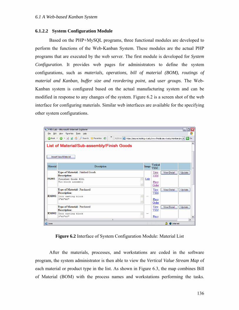
6.1 A Web-based Kanban System
6.1.2.2 System Configuration Module
Based on the PHP+MySQL programs, three functional modules are developed to
perform the functions of the Web-Kanban System. These modules are the actual PHP
programs that are executed by the web server. The first module is developed for System
Configuration. It provides web pages for administrators to define the system
configurations, such as materials, operations, bill of material (BOM), routings of
material and Kanban, buffer size and reordering point, and user groups. The Web-
Kanban system is configured based on the actual manufacturing system and can be
modified in response to any changes of the system. Figure 6.2 is a screen shot of the web
interface for configuring materials. Similar web interfaces are available for the specifying
other system configurations.
Figure 6.2 Interface of System Configuration Module: Material List
After the materials, processes, and workstations are coded in the software
program, the system administrator is then able to view the Vertical Value Stream Map of
each material or product type in the list. As shown in Figure 6.3, the map combines Bill
of Material (BOM) with the process names and workstations performing the tasks.
136
6.1 A Web-based Kanban System
Authorized users can place orders of selected material by using this interface. With
specified quantity and duedate, the order will be transformed into Kanbans (one for each
unit) to trigger the jobs. A pull system is embedded in the design, and materials are pulled
from upstream workstations when needed. The orders can be placed in Batches (pulling
multiple units all at once) or Leveled Pulling (evenly spreads the order amount over a
period of time) to the selected workstation. When the demand is leveled, the Kanban will
be dispatched automatically over the specified period, and thus the chance of human
errors on timing can be minimized.
Figure 6.3 Interface of System Configuration Module: Order Placement
137

6.1 A Web-based Kanban System
6.1.2.3 Kanban Operating Module
Following the system configuration module is the Kanban Operating Module. It
provides interfaces for operators at the workstations to receive, process, and fulfill the
Kanbans. When the system configuration is completed, users at each workstation can log
on to the system to view the designated Kanbans. Based on the predefined user groups
and authority levels, only the authorized user can see the designated Kanbans and
information from the operating page.
After logging into the system, a job list will be provided to the user. As shown in
Figure 6.4, new jobs, in-process jobs, pending jobs, and completed jobs are listed for the
user to view or execute. An orange “►” button is displayed on every Kanban operating
page to identify the task of highest priority. Therefore, the operator can follow the button
to execute the jobs in the order of urgency.
Figure 6.4 Interface of Kanban Operating Module: Job List
138
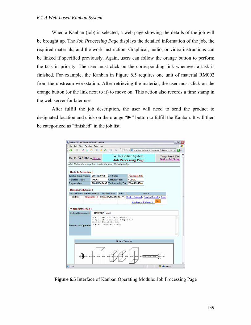
6.1 A Web-based Kanban System
When a Kanban (job) is selected, a web page showing the details of the job will
be brought up. The Job Processing Page displays the detailed information of the job, the
required materials, and the work instruction. Graphical, audio, or video instructions can
be linked if specified previously. Again, users can follow the orange button to perform
the task in priority. The user must click on the corresponding link whenever a task is
finished. For example, the Kanban in Figure 6.5 requires one unit of material RM002
from the upstream workstation. After retrieving the material, the user must click on the
orange button (or the link next to it) to move on. This action also records a time stamp in
the web server for later use.
After fulfill the job description, the user will need to send the product to
designated location and click on the orange “►” button to fulfill the Kanban. It will then
be categorized as “finished” in the job list.
Figure 6.5 Interface of Kanban Operating Module: Job Processing Page
139

6.1 A Web-based Kanban System
6.1.2.4 Performance Monitoring Module
The last functional module of the Web-Kanban System is for managers to monitor
and analyze the performance dispatched jobs. Currently, this module offers the functions
of Kanban Tracking, Work-in-Process (WIP) Level Monitoring, and Time-based
Performance Analysis. Also, the time stamps can be output to the Excel-based DEA
Solver for leanness measurement. Extensions of the functionality are discussed in the
next section.
In the Kanban Tracking interface, the quantity, status and timing of the Kanbans
are listed for the system manager. As shown in Figure 6.6, the managers can view the list
of Inactive (finished or scrapped) or Active (new, in-process, or reworking) Kanbans.
Details of each can be can also be found by following the links provided in the web page.
Figure 6.7 demonstrates the Vertical Value Stream that shows the WIP level of each
material involved. Managers can identify problematic areas of the value stream where
high WIP level is shown. In Figure 6.8, the time-based performance of each Kanban is
displayed. Accumulated time and accumulated VA time are listed together with a
graphical display of the VA time versus NVA time of each job. The time stamps of VA
and NVA activities are recorded in the web server, which are used to build ADMUs and
IDMUs for the DEA-Leanness Measure.
Figure 6.6 Interface of Performance Monitoring Module: Kanban Tracking
140

6.1 A Web-based Kanban System
Figure 6.7 Interface of Performance Monitoring Module: WIP Level Monitoring
Figure 6.8 Interface of Performance Monitoring Module: Time-based Performance
141

6.1 A Web-based Kanban System
6.1.3 Discussions on Web-Kanban System
The Web-Kanban System provides a way to collect time-based data automatically.
It is designed to be applicable to various environments; however the scope of application
is still limited. First, it is not necessary to implement the Web-Kanban System if a
computer-based system (such as ERP system) is already in place that can monitor and
record the time-based performance. Furthermore, the Web-Kanban is not applicable if
network connection is not available at the workstations. Besides, when the cycle time of a
process is short, clicking on the web pages may become a burden for the operators.
Therefore, the Web-Kanban is suitable for manufacturing systems where delicate
computer system is not available; network is accessible at workstations; and the work
pieces flow through the system in a moderate pace. Comparing to manual data collection,
when multiple products are in the system simultaneously, a dedicated observer may not
be sufficient. In that situation, the Web-Kanban System provides a solution.
Beside the scope of application, the functionality of the Web-kanban System is
limited in the following areas:
1) Model Solving: The web-based technology provides certain level of computational
power, but the capability of solving mathematical programs is limited. Although the
SBM model can be transformed into a linear program and solved by using Simplex
Method, the solver needs to be programmed from scratch. The solution in this
research is to feed the data collected by Web-Kanban to the Excel-based program,
which provides various built-in features for data analysis.
2) Graphical Display: The standard HTML web pages are capable of displaying
various types of data, such as text, image, audio, and video. However, the charts of
data analysis, which can be easily generated by spreadsheet packages, are not
included. Advanced web-based programming tools, such as Macromedia Flash, can
be the solution in the future.
3) Interface: Current version of the Web-Kanban System cannot work with other
software packages due to lacking of interfacing programs. If the interfaces can be
built to link the Web-Kanban with other shop floor control programs or data analysis
programs, it would improve the applicability of the system dramatically. More
142
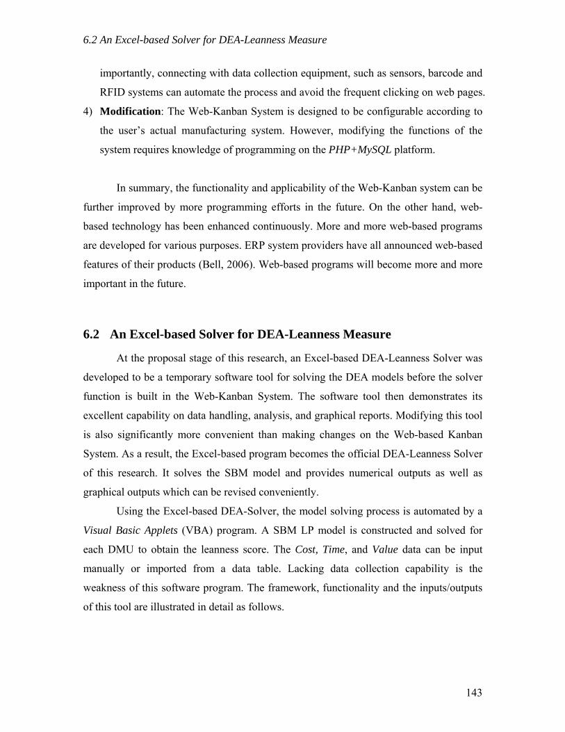
6.2 An Excel-based Solver for DEA-Leanness Measure
importantly, connecting with data collection equipment, such as sensors, barcode and
RFID systems can automate the process and avoid the frequent clicking on web pages.
4) Modification: The Web-Kanban System is designed to be configurable according to
the user’s actual manufacturing system. However, modifying the functions of the
system requires knowledge of programming on the PHP+MySQL platform.
In summary, the functionality and applicability of the Web-Kanban system can be
further improved by more programming efforts in the future. On the other hand, web-
based technology has been enhanced continuously. More and more web-based programs
are developed for various purposes. ERP system providers have all announced web-based
features of their products (Bell, 2006). Web-based programs will become more and more
important in the future.
6.2 An Excel-based Solver for DEA-Leanness Measure
At the proposal stage of this research, an Excel-based DEA-Leanness Solver was
developed to be a temporary software tool for solving the DEA models before the solver
function is built in the Web-Kanban System. The software tool then demonstrates its
excellent capability on data handling, analysis, and graphical reports. Modifying this tool
is also significantly more convenient than making changes on the Web-based Kanban
System. As a result, the Excel-based program becomes the official DEA-Leanness Solver
of this research. It solves the SBM model and provides numerical outputs as well as
graphical outputs which can be revised conveniently.
Using the Excel-based DEA-Solver, the model solving process is automated by a
Visual Basic Applets (VBA) program. A SBM LP model is constructed and solved for
each DMU to obtain the leanness score. The Cost, Time, and Value data can be input
manually or imported from a data table. Lacking data collection capability is the
weakness of this software program. The framework, functionality and the inputs/outputs
of this tool are illustrated in detail as follows.
143
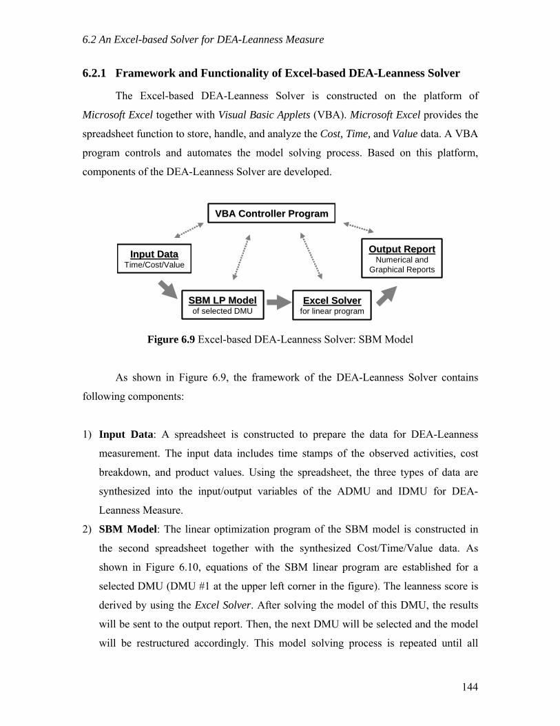
6.2 An Excel-based Solver for DEA-Leanness Measure
6.2.1 Framework and Functionality of Excel-based DEA-Leanness Solver
The Excel-based DEA-Leanness Solver is constructed on the platform of
Microsoft Excel together with Visual Basic Applets (VBA). Microsoft Excel provides the
spreadsheet function to store, handle, and analyze the Cost, Time, and Value data. A VBA
program controls and automates the model solving process. Based on this platform,
components of the DEA-Leanness Solver are developed.
Input DataInput DataTime/Cost/Value
SBM LP ModelSBM LP Modelof selected DMU
Excel SolverExcel Solverfor linear program
VBA Controller ProgramVBA Controller Program
Output ReportOutput ReportNumerical and
Graphical Reports
Input DataInput DataTime/Cost/Value
SBM LP ModelSBM LP Modelof selected DMU
Excel SolverExcel Solverfor linear program
VBA Controller ProgramVBA Controller Program
Output ReportOutput ReportNumerical and
Graphical Reports
Figure 6.9 Excel-based DEA-Leanness Solver: SBM Model
As shown in Figure 6.9, the framework of the DEA-Leanness Solver contains
following components:
1) Input Data: A spreadsheet is constructed to prepare the data for DEA-Leanness
measurement. The input data includes time stamps of the observed activities, cost
breakdown, and product values. Using the spreadsheet, the three types of data are
synthesized into the input/output variables of the ADMU and IDMU for DEA-
Leanness Measure.
2) SBM Model: The linear optimization program of the SBM model is constructed in
the second spreadsheet together with the synthesized Cost/Time/Value data. As
shown in Figure 6.10, equations of the SBM linear program are established for a
selected DMU (DMU #1 at the upper left corner in the figure). The leanness score is
derived by using the Excel Solver. After solving the model of this DMU, the results
will be sent to the output report. Then, the next DMU will be selected and the model
will be restructured accordingly. This model solving process is repeated until all
144
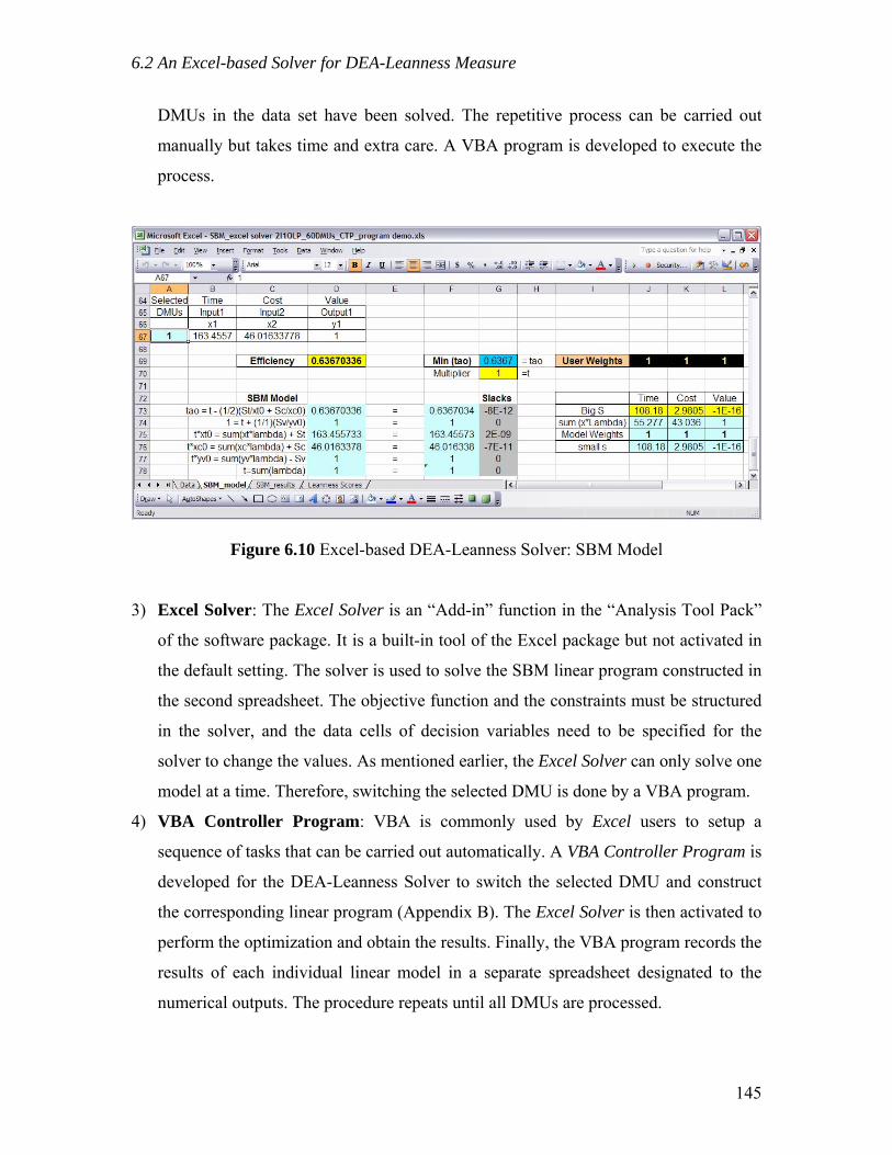
6.2 An Excel-based Solver for DEA-Leanness Measure
DMUs in the data set have been solved. The repetitive process can be carried out
manually but takes time and extra care. A VBA program is developed to execute the
process.
Figure 6.10 Excel-based DEA-Leanness Solver: SBM Model
3) Excel Solver: The Excel Solver is an “Add-in” function in the “Analysis Tool Pack”
of the software package. It is a built-in tool of the Excel package but not activated in
the default setting. The solver is used to solve the SBM linear program constructed in
the second spreadsheet. The objective function and the constraints must be structured
in the solver, and the data cells of decision variables need to be specified for the
solver to change the values. As mentioned earlier, the Excel Solver can only solve one
model at a time. Therefore, switching the selected DMU is done by a VBA program.
4) VBA Controller Program: VBA is commonly used by Excel users to setup a
sequence of tasks that can be carried out automatically. A VBA Controller Program is
developed for the DEA-Leanness Solver to switch the selected DMU and construct
the corresponding linear program (Appendix B). The Excel Solver is then activated to
perform the optimization and obtain the results. Finally, the VBA program records the
results of each individual linear model in a separate spreadsheet designated to the
numerical outputs. The procedure repeats until all DMUs are processed.
145
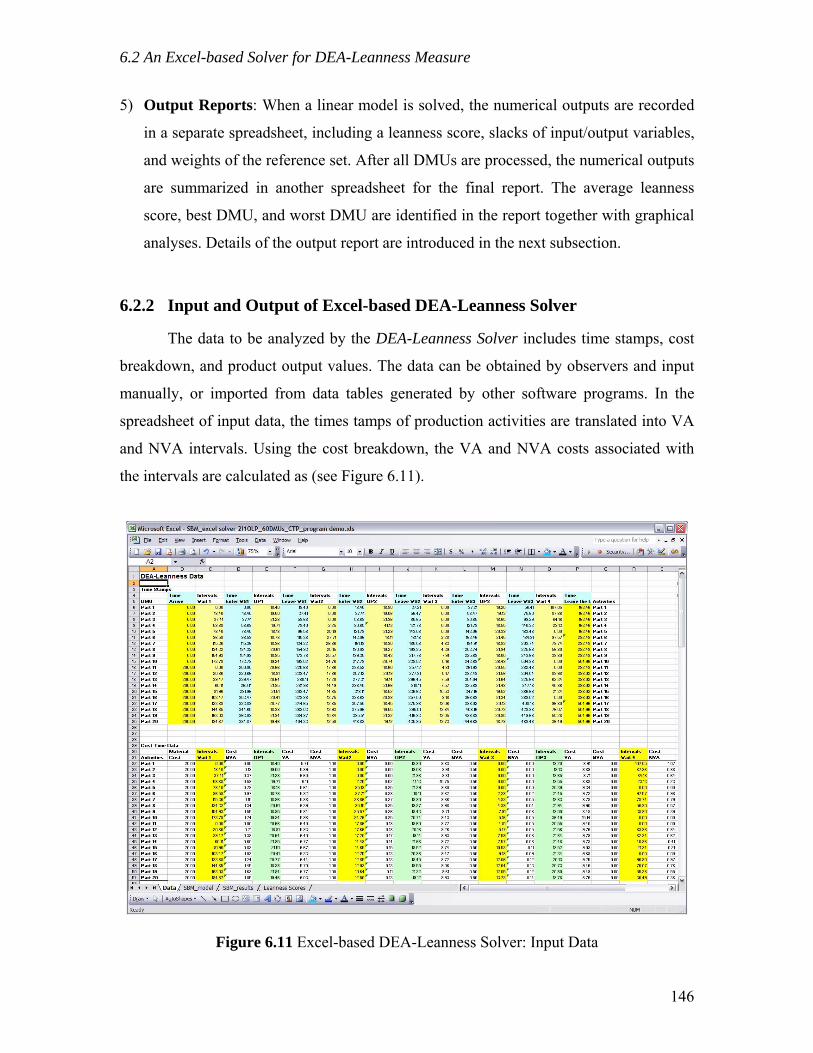
6.2 An Excel-based Solver for DEA-Leanness Measure
5) Output Reports: When a linear model is solved, the numerical outputs are recorded
in a separate spreadsheet, including a leanness score, slacks of input/output variables,
and weights of the reference set. After all DMUs are processed, the numerical outputs
are summarized in another spreadsheet for the final report. The average leanness
score, best DMU, and worst DMU are identified in the report together with graphical
analyses. Details of the output report are introduced in the next subsection.
6.2.2 Input and Output of Excel-based DEA-Leanness Solver
The data to be analyzed by the DEA-Leanness Solver includes time stamps, cost
breakdown, and product output values. The data can be obtained by observers and input
manually, or imported from data tables generated by other software programs. In the
spreadsheet of input data, the times tamps of production activities are translated into VA
and NVA intervals. Using the cost breakdown, the VA and NVA costs associated with
the intervals are calculated as (see Figure 6.11).
Figure 6.11 Excel-based DEA-Leanness Solver: Input Data
146
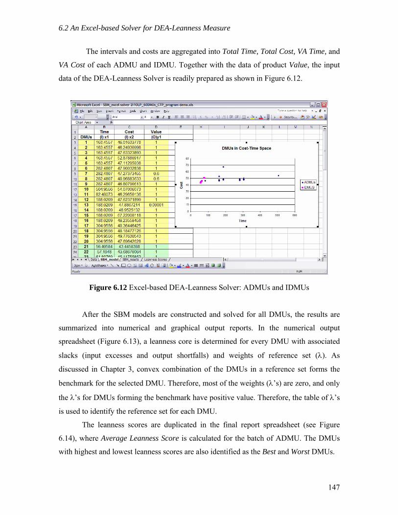
6.2 An Excel-based Solver for DEA-Leanness Measure
The intervals and costs are aggregated into Total Time, Total Cost, VA Time, and
VA Cost of each ADMU and IDMU. Together with the data of product Value, the input
data of the DEA-Leanness Solver is readily prepared as shown in Figure 6.12.
Figure 6.12 Excel-based DEA-Leanness Solver: ADMUs and IDMUs
After the SBM models are constructed and solved for all DMUs, the results are
summarized into numerical and graphical output reports. In the numerical output
spreadsheet (Figure 6.13), a leanness core is determined for every DMU with associated
slacks (input excesses and output shortfalls) and weights of reference set (λ). As
discussed in Chapter 3, convex combination of the DMUs in a reference set forms the
benchmark for the selected DMU. Therefore, most of the weights (λ’s) are zero, and only
the λ’s for DMUs forming the benchmark have positive value. Therefore, the table of λ’s
is used to identify the reference set for each DMU.
The leanness scores are duplicated in the final report spreadsheet (see Figure
6.14), where Average Leanness Score is calculated for the batch of ADMU. The DMUs
with highest and lowest leanness scores are also identified as the Best and Worst DMUs.
147
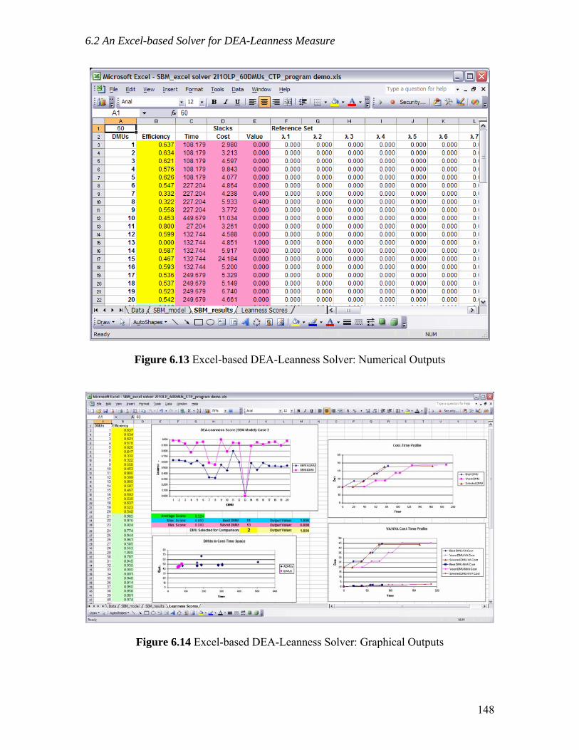
6.2 An Excel-based Solver for DEA-Leanness Measure
Figure 6.13 Excel-based DEA-Leanness Solver: Numerical Outputs
Figure 6.14 Excel-based DEA-Leanness Solver: Graphical Outputs
148

6.2 An Excel-based Solver for DEA-Leanness Measure
In the reporting spreadsheet (Figure 6.14), a line chart shows the leanness scores
graphically. The ADMUs and IDMUs are plotted in a scatter diagram in the Cost-Time
space for comparison. In addition, a Cost-Time-Profile (CTP) with Total Cost (Figure
6.15) and a CTV Chart with VA and NVA Costs (Figure 6.16) are plotted with the Best
ADMU, Worst ADMU, and a selected DMU. Using the CTP and CTV charts, the
profiles of production processes are compared to identify potential improvements as
discussed in Section 4.3.
Cost-Time Profile
0
10
20
30
40
50
60
0 20 40 60 80 100 120 140 160 180 200
Time
Cos
t Best DMUWorst DMUSelected DMU
Figure 6.15 Excel-based DEA-Leanness Solver: Cost-Time Profile
Cost-Time-Value Chart
05
101520253035404550
0 50 100 150 200
Time
Cos
t
Best DMU-VA CostWorst DMU-VA CostSelected DMU-VA CostBest DMU-NVA CostWorst DMU-NVA CostSelected DMU-NVA Cost
Figure 6.16 Excel-based DEA-Leanness Solver: VA vs. NVA Costs
149
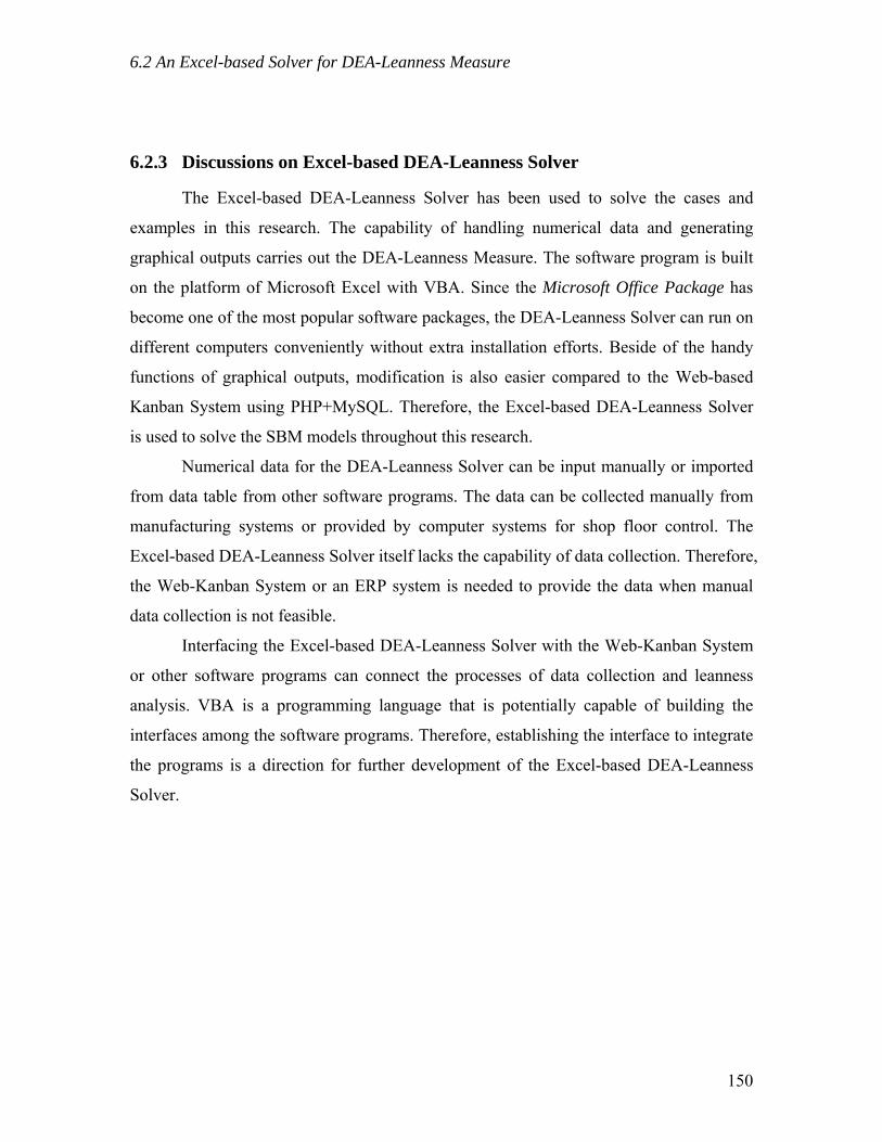
6.2 An Excel-based Solver for DEA-Leanness Measure
6.2.3 Discussions on Excel-based DEA-Leanness Solver
The Excel-based DEA-Leanness Solver has been used to solve the cases and
examples in this research. The capability of handling numerical data and generating
graphical outputs carries out the DEA-Leanness Measure. The software program is built
on the platform of Microsoft Excel with VBA. Since the Microsoft Office Package has
become one of the most popular software packages, the DEA-Leanness Solver can run on
different computers conveniently without extra installation efforts. Beside of the handy
functions of graphical outputs, modification is also easier compared to the Web-based
Kanban System using PHP+MySQL. Therefore, the Excel-based DEA-Leanness Solver
is used to solve the SBM models throughout this research.
Numerical data for the DEA-Leanness Solver can be input manually or imported
from data table from other software programs. The data can be collected manually from
manufacturing systems or provided by computer systems for shop floor control. The
Excel-based DEA-Leanness Solver itself lacks the capability of data collection. Therefore,
the Web-Kanban System or an ERP system is needed to provide the data when manual
data collection is not feasible.
Interfacing the Excel-based DEA-Leanness Solver with the Web-Kanban System
or other software programs can connect the processes of data collection and leanness
analysis. VBA is a programming language that is potentially capable of building the
interfaces among the software programs. Therefore, establishing the interface to integrate
the programs is a direction for further development of the Excel-based DEA-Leanness
Solver.
150

7.1 Summary and Conclusions
Chapter 7 Conclusions
7.1 Summary and Conclusions
The objective of this research is to develop a leanness measure for manufacturing
systems that tells lean practitioners “how lean their system is” and “how lean it should
be.” Since the late 1990’s, lean manufacturing has become one of the most popular
improvement strategies for manufacturing systems. The “waste elimination” concept is
simple yet effective for manufacturing systems and various other settings. Earlier tools
and techniques developed for implementing lean concepts focus mostly on “how to make
the system leaner.” Specific problems are tackled by these tools and techniques, and the
visible improvements of performance can be achieved. Using performance metrics, the
improvements can be quantified to justify the implementation of lean manufacturing.
However, the conventional lean metrics cannot tell the lean practitioners how lean their
system is, how much leaner it can be, or how lean it should be.
In this research, a DEA-Leanness Measure has been developed to quantify the
leanness level of manufacturing systems. The DEA technique evaluates performance of
DMUs by comparing the outputs/inputs ratio of each DMU. Most efficient DMUs form
the efficiency frontier, which provides a benchmark for every DMU to quantify its
performance. Using virtually generated IDMUs, the leanness frontier is pushed towards
an ideally lean stage. Thus, leanness scores of the DMUs can be calculated by comparing
the DMUs against the frontier. A CCR model is originally used to perform the DEA-
Leanness measurement. However, the scores of CCR model overestimate the leanness
level whenever slacks (i.e., input excesses or output shortfalls) exist in a benchmark.
From the hypothetical cases, it is found that the slacks exist frequently while measuring
leanness of manufacturing systems. A SBM model is then adapted to replace the CCR
model. The DEA-Leanness Measure using SBM model effectively identifies the leanness
benchmark and calculates the leanness scores accordingly. Through hypothetical cases,
the results obtained from the SBM model are proven to be more accurate than the CCR
model. Therefore, the DEA-Leanness Measure is developed based on SBM model.
151

7.1 Summary and Conclusions
Using the DEA-Leanness Measure, leanness level of manufacturing systems can
be quantified and compared. It is an indication of “how lean the system is.” On the other
hand, it tells practitioners “how much leaner” the system can be, because the leanness
score is obtained by comparing against a perfectly lean state.
Performing the DEA-Leanness measurement requires detailed Cost, Time, and
Value data of every DMU. Collecting, handling and analyzing the large amount of data
may require extra time and effort. Two software programs are then developed to perform
these tasks. A Web-Kanban System is developed to facilitate the data collection. It is a
computerized Kanban system enabled by web-based technology. Using the system, the
time stamps of every activity can be recorded and then translated into VA and NVA time
spans for forming the ADMUs and IDMUs. After the required data is collected, the
leanness scores can be derived by an Excel-based DEA-Leanness Solver. The solver is
developed to solve the SBM models of the DMUs and generate the leanness scores. CTP
of the DMUs with VA, NVA and total costs are generated automatically for the users to
identify potential improvements.
The abovementioned two software programs are developed to handle large
amount of DMUs. However, there are situations that only very little data can be obtained.
The application of DEA-Leanness Measure using VSM data is explored. It has been
demonstrated that as long as corresponding Costs and product Value can be identified, the
leanness level of a value stream can be measured based on the averages of time-based
performance found in a VSM. The SBM model is capable of generating a reasonable
leanness score using one pair of ADMU and IDMU. This application is useful for the
scenarios where detailed data is hard to obtained, such as manufacturing systems with
extremely short cycle time or complicated supply chains.
The DEA-Leanness Measure can also be an index for decision makers to compare
the effectiveness of different improvement initiatives. Tradeoffs between the initiatives
can be quantified using the leanness scores. Furthermore, weights can be applied to the
input/output variables (i.e., Cost, Time, and Value) of the leanness measure so that the
Weighted DEA-Leanness Measure can reflect the performance changes with
consideration of the company’s focus. Consequently, companies adapting different
competitive strategies can establish leanness measures that match their needs.
152
7.1 Summary and Conclusions
With the ability of measuring leanness, the next question to be answered is “how
lean the system should be.” A methodology is developed in this research to identify the
leanness target considering unavoidable delays in and out of the manufacturing system.
Internally, the imbalance between production processes delays the flow of products
inevitably. For this situation, an Online-delay target is identified based on the concept of
“supermarket pulling system” developed by Toyota. On the other hand, the fluctuation of
demand cannot always be addressed by adjusting the pace of production. Inventory or
working overtime is necessary to satisfy the customers with an acceptable agility level.
An Offline-delay target is developed to represent the necessary inventory level to address
the demand fluctuation. Combining the two targets, a leanness target can be identified for
certain level of agility. Based on the leanness target, the Lean-Agile Performance Index
shows whether the system is lean enough for the desired level of agility.
In conclusion, a DEA-Leanness Measure is developed to quantify leanness level
of manufacturing systems, which reflects the current state of a system against perfection,
and a leanness target can be identified for desired agility level. The effectiveness of the
leanness measure has been verified by hypothetical cases. Certain limitations associated
with the methodologies developed in this research are listed as follows.
1) Scope of the Measure: The DEA-Leanness Measure can be applied to different
levels of a manufacturing system. However, the scope of application and
granulation of details included in the input/output variables affect the result of
leanness measurement. In a single workstation or a small production cell,
transportation, buffering and other NVA activities are expected to be less than
those in a complicated production line or a whole factory. As a result, the leanness
scores associated with smaller scopes are expected to be higher than the overall
score of a large scope. Therefore, when two systems are compared using the
leanness score, the scope of the applications should be kept in mind while
interpreting the difference of the scores.
2) Granulation of the Input Data: The granulation of details of the input data also
affects the accuracy of the measure. While analyzing the VA and NVA
components of the production processes, including finer details tends to identify
153
7.1 Summary and Conclusions
more NVA cost and time from an activity since wastes can be hidden in the VA
activities. For example, if the time and cost spent in a workstation are considered
as fully value-adding, then the time wasted on load/unload and the cost of
scrapped material are mislabeled, and the leanness score would be overestimated.
Similarly for the leanness measure of a supply chain, the cost and time spent in
one plant should not be considered all VA. Keeping a finer granulation of the
input data can deliver a more accurate leanness score and more importantly, helps
the lean practitioners identify more opportunities of improvement.
3) Evaluation of Product Value: The output variable, Value, of DMU is designed
to reflect the customers’ perception of the product. Unlike the cost and time data,
some components of customer satisfaction can only be evaluated qualitatively.
Subjective judgments can sometimes affect the results of the leanness measure.
For example, if one of ten customers is unsatisfied with a product and the one is
included in a sample of two customers, the result will be quite different from the
fact. Nevertheless, following up the satisfaction rate of every customer is not
always possible. An appropriate sample size should be obtained to deliver more
reasonable evaluation of customer satisfaction.
4) Identification of Improvements: The CTP with VA and NVA costs provide a
way to identify wastes in the production processes. However, some wastes may
not be trivially visible in the chart. The CTV analysis may shed a light on
potential improvements by comparing costs and time spans, but more
improvement opportunities may be hidden in the charts. Detailed investigation on
the value stream is still the most effective way to identify wastes and further
improve the system.
The contributions of this research and potential directions of future research are
discussed in the following two sections.
154

7.2 Contributions of this Research
7.2 Contributions of this Research
The major accomplishment of this research is the development of a quantitative
leanness measure for manufacturing systems based on DEA technique. Unlike the
conventional lean manufacturing tools and techniques, the DEA-Leanness Measure helps
lean practitioners understand “how lean the system is” as well as “how lean it should be.”
The contributions of this research to the development and implementation of lean
manufacturing are listed below.
1) An Integrated Index of Leanness of Manufacturing Systems: The DEA-
Leanness Measure provides an integrated index of leanness level, which
eliminates the need to interpret several lean metrics at the same time. The Cost,
Time, and Value variables are considered simultaneously in the measure, and a
unit-invariant score between 0 and 1 is provided. It provides the information on
how much waste can possibly be removed from the current system in order to get
to the ideal leanness. The measure can be applied to different scopes of systems,
and the self-contained leanness benchmark eliminates the need to outsource the
performance standard repeatedly
2) A Weighted Leanness Measure Considering Competitive Strategies: The
DEA-Leanness Measure can take different weights assigned to the input/output
variables (i.e., Cost, Time and Value). The resulting leanness score can reflect the
performance of the system or the impact of improvement initiatives considering
the competitive focus of the company.
3) Leanness Target Identification Considering Agility Level: An appropriate
leanness level considering desirable agility level can be identified based on the
DEA-Leanness Measure. Acceptable delays in a manufacturing system or in
inventory are identified to form the leanness target that tells lean practitioners
“how lean the system should be.”
4) Potential Improvements Identification: The Cost-Time-Value analysis
developed in this research provides a way to identify potential improvements by
comparing the Cost-Time Profiles of different DMUs.
155
7.3 Future Research Areas
5) A Web-based Kanban System: A computerized Kanban system is developed
using web-based technology. Comparing to existing proprietary ERP or MES
systems, the Web-Kanban System demonstrates a possibility to computerize the
shop floor control simply using web services and standard web browsers. On the
other hand, the web-based system enhanced the functionality of Kanban system
by adding the capability of Kanban tracking and monitoring. The time-based data
can be recorded in detail and analyzed by the web server. Performance of the
system can then be monitored by authorized users in real time.
7.3 Future Research Areas
The goal of this research is to develop a methodology to help lean manufacturing
practitioners implement lean concepts in a more efficient and more effective way. The
solution provided by this research is a leanness measure that tells the lean practitioners
“how lean the system is,” “how lean it should be,” and eventually “how to achieve the
desired leanness level.” In the future, the methodology can be further enhanced in the
following areas.
1) Empirical Study on Real-World Systems: The approaches developed in this
research are verified using hypothetical cases. Case studies based on real
manufacturing system should be carried out to verify and improve the
methodology. The case studies should include leanness measure and target
identification for manufacturing systems, leanness measure using VSM, weighted
leanness measure for different strategies, and improvement direction
identification using CTP. Carrying out the case studies can help lean practitioners
gain more insight into the performance of their systems and the impacts of the
lean initiatives. Meanwhile, potential enhancements of the leanness measure can
be explored.
2) Including Cost-Time Investment (CTI) in the Leanness Measure: In the CTP
approach, the CTI (area under the curve) represents the time-value of monetary
investments. The objective to minimize CTI supports the Just-in-Time strategy
156
7.3 Future Research Areas
and the postponement of product differentiation in agile manufacturing. However,
the current DEA-Leanness Measure can hardly capture this characteristic since
the cost and time variables are separated. Revising the leanness measure to
include CTI as part of the input data may deliver a performance index that
identifies competitive advantages more effectively.
3) Applying DEA-Leanness Measure on Other Environments: The proposed
leanness measure is developed mainly for manufacturing systems. The same
methodology can possibly be applied to other circumstance, such as service
sectors, administrative works, research and development, etc. The way to identify
input/output variables and collecting appropriate data needs to be further
investigated.
4) Developing Leanness Target for Various Scenarios: Currently, the lean-agile
target is represented by a leanness score considering the imbalance within a
manufacturing system and the fluctuation of demand. The quantity and variability
of customer’s demand is taken as the requirement of agility, and inventory is
assumed to be the solution to address the agility. Besides, the imbalances between
workstations are assumed to be unchangeable. In reality, fluctuation in demand
can also be addressed by other actions, such as working overtime or outsourcing.
On the other hand, imbalances in the production line can be improved by
reengineering. The target of lean-agile performance should be further investigated
in order to develop a better methodology to help lean practitioners understand
“how lean the system should be” and “how to achieve the leanness.”
5) Constructing Web-based Manufacturing System: A Web-Kanban system has
been developed in this research to explore the possibility of computerizing the
Kanban system with web services and standard web browser. Although the
software program does not possess many functions, the simplicity and
effectiveness of web-based infrastructure demonstrates potential impacts on the
information system for manufacturing. Actually, web-based technology has been
improved dramatically in the past decade and will be further reinforced
continuously. The capability of real-time data collection and analysis and the
accessibility of online information have made web-based programming a trend for
157
7.3 Future Research Areas
the next generation of information system for manufacturing. The Web-Kanban
System can be further enhanced by adding the interfaces with data collection
devices and other computer programs for manufacturing systems. Also, leanness
measurement and other performance metrics can be built into the Web-Kanban
System. In the near future, developing “Performance-based Manufacturing
Systems” with web-based technology should be a promising area for research.
The Lean Manufacturing concepts continue to be the most popular improvement
strategy for manufacturing systems in 21st century. Furthermore, the Lean Thinking has
been expanded to cover various settings beyond manufacturing. The service sectors,
administrative works, health care systems and many other systems have all been explored
by supporters of lean thinking, and the results are impressive reportedly. This research
provides a novel approach to measure leanness level of manufacturing systems. The
effort is expected to bring impacts and contributions to the research and applications of
lean concepts. Hopefully, the ideas and methodologies will inspire more research in this
area to reinforce the impact of lean concepts continuously.
158
References
References
Achour, M., Betz, F., Dovgal, A., Lopes, N., Olson, P., Richter, G., Seguy, D., and Vrana, J., 2006, PHP Manual, PHP Documentation Group, (http://php.net).
Aitken, J., Christopher, M., and Towill, D., 2002, “Understanding, Implementing and Exploiting Agility and Leanness,” International Journal of Logistics, 5(1), 59-75.
Allen, J., Robinson, C., and Stewart, D., 2001, Lean Manufacturing: A plant floor guide, Society of Manufacturing Engineers, Dearborn, MI.
Arbos, L. C., 2002, “Design of a rapid response and high efficiency service by lean production principles: Methodology and evaluation of variability of performance,” International Journal of Production Economics, 80, 169-183.
Arteta, B. M. and Giachetti, R. E., 2004, “A measure of agility as the complexity of the enterprise system,” Robotics and Computer-Integrated Manufacturing, 20, 495-503.
Atkinson, L., 2002, Core MySQL, Prentice Hall, Upper Saddle River, NJ.
Babu, A. S., Nandurkar, K. N., and Thomas, A., 2000, “Development of virtual cellular manufacturing systems for SMEs,” Logistics Information Management, 13(4), 228-242.
Baykasoglu, A., 2003, “Capability-based distributed layout approach for virtual manufacturing cells,” International Journal of Production Research, 41(11), 2597-2618.
Bell, S., 2006, Lean Enterprise Systems: Using IT for Continuous Improvement, John Wiley & Sons, Hoboken, NJ.
Boussofiane, A., Dyson, R. G., and Thanassoulis, E., 1991, “Applied Data Envelopment Analysis,” European Journal of Operational Research, 52, 1-15.
Callen, J. L., Fader, C., and Krinsky, I., 2000, “Just-in-time: a cross-sectional plant analysis,” International Journal of Production Economics, 63, 277-301.
Charnes, A., Clark, T., Cooper, W. W., and Golany, B., 1985, “An envelopment study of data envelopment analysis in measuring the efficiency of maintenance units in the U.S. air forces,” Annals of Operations Research, 2, 95-112.
Charnes, A., Cooper, W. W., and Rhodes, E., 1978, “Measuring the efficiency of decision making units,” European Journal of Operational Research, 2(6), 429-444.
Christopher, M. and Towill, D. R., 2000, “Supply chain migration from lean and functional to agile and customised,” Supply Chain Management: An International Journal, 5(4), 206-213.
159
References
Comm, C. L. and Mathaisel, D. F. X., 2000, “A paradigm for benchmarking lean initiatives for quality improvement,” Benchmarking: An International Journal, 7(2), 118-127.
Conner, G., 2001, Lean Manufacturing for the Small Shop, Society of Manufacturing Engineers, Dearborn, MI.
Cooper, W. W., Seiford, L. M., and Tone, K., 2004, Data Envelopment Analysis, 4th edition, Kluwer Academic Publishers, Boston, MA.
Detty, R. B., and Yingling, J. C., 2000, “Quantifying benefits of conversion to lean manufacturing with discrete event simulation: a case study,” International Journal of Production Research, 38(2), 429-445.
Duggan, K. J., 2002, Creating Mixed Model Value Streams, Productivity Press, New York, NY.
Feld, W. M., 2000, Lean Manufacturing: Tools, Techniques, and How to Use Them, The St. Lucie Press/APICS Series on Resource Management, Alexandria, VA.
Fogarty, D. W., 1992, “Work in process: performance measures,” International Journal of Production Economics, 26, 169-172.
Fooks, J. H., 1993, Profiling for Performance: Total Quality Methods for Reducing Cycle Time, Addison-Wesley, Reading, MA.
Goldman, S. L., Nagel R. N., and Preiss, K., 1995, Agile Competitors and Virtual Organizations, Van Nostrand Reinhold, New York, NY.
Goranson, H. T., 1999, The Agile Virtual Enterprise: Cases, Metrics, Tools, Quorum Books, London.
Gunasekaran, A. and Yusuf, Y. Y., 2002, “Agile manufacturing: a taxonomy of strategic and technological imperatives,” International Journal of Production Research, 40(6), 1357-1385.
Helo, P., 2004, “Managing agility and productivity in the electronics industry,” Industrial Management and Data Systems, 104(7), 567-577.
Hopp. W. J. and Spearman, M. L., 2000, Factory Physics: Foundations of Manufacturing Management, McGraw-Hill, New York, NY.
Jackson, M. and Johansson, C., 2003, “An agility analysis from a production system perspective,” Integrated Manufacturing Systems, 14(6), 482-488.
Jina, J., Bhattacharya, A. K., and Walton, A. D., 1997, “Applying lean principles for high product variety and low volumes: some issues and propositions,” Logistics Information Management, 10 (1), 5-13.
160
References
Johansson, H. J., McHugh, P., Pendlebury, A. J., and Wheeler, W. A., 1993, Business Process Reengineering: Breakpoint strategies for Market Dominance, John Wiley and Sons, Chichester, UK.
Jones, D. T. and Womack, J. P., 2002, Seeing the Whole: Mapping the Extended Value Stream, Lean Enterprise Institute, Inc., Brookline MA.
Jordan, J. A., Jordan, J. A., Jr., and Michel, F. J., 2001, The Lean Company: Making the Right Choices, Society of Manufacturing Engineering, Dearborn, MI.
Kaplan, R. S. and Norton, D. P., 1992, “The Balanced Scorecard – measures that drive performance,” Harvard Business Review, January-February, 70-79.
Karlsson, C. and Ahlstrom, P., 1996, “Assessing changes towards lean production,” International Journal of Operations and Production Management, 16(2), 24-41.
Katayama, H. and Bennett, D., 1999, “Agility, adaptability and leanness: A comparison of concepts and a study of practice,” International Journal of Production Economics, 60-61, 43-51.
Leung, S. and Lee W. B., 2004, “Strategic manufacturing capability pursuance: a conceptual framework,” Benchmarking: An International Journal, 11(2), 156-174.
Levinson, W. A. and Rerick, R. A., 2002, Lean Enterprise: A synergistic approach to minimizing waste, American Society for Quality, Milwaukee, WI.
Maskell, B. and Baggaley, B., 2004, Practical Lean Accounting, Productivity Press, New York , NY.
Mason-Jones, R., Naylor, B., and Towill, D. R., 2000a, “Engineering the leagile supply chain,” International Journal of Agile Management Systems, 2(1), 54-61.
Mason-Jones, R., Naylor, B., and Towill, D. R., 2000b, “Lean, agile or leagile? Matching your supply chain to the marketplace,” International Journal of Production Research, 38(17), 4061-4070.
McIvor, R., 2001, “Lean supply: the design and cost reduction dimensions,” European Journal of Purchasing and Supply Management, 7, 227-242.
Monden, Y., 1998, Toyota Production System: an integrated approach to just-in-time, 3rd edition, Institute of Industrial Engineers, Norcross, GA.
Naylor, J. B., Naim, M. M., and Berry, D., 1999, “Leagility: Integrating The Lean and Agile Manufacturing Paradigms in The Total Supply Chain,” International Journal of Production Economics, 62, 107-118.
Ohno, T., 1988, Toyota Production System, Productivity Press, Portland, OR.
161

References
Prince, J. and Kay, J. M., 2003, “Combining lean and agile characteristics: Creation of virtual groups by enhanced production flow analysis,” International Journal of Production Economics, 85, 305-318.
Radnor, Z. J. and Boaden, R., 2004, “Developing and understanding of corporate anorexia,” International Journal of Operations and Production Management, 24(4), 424-440.
Ramasesh, R., Kulkarni, S., and Jayakumar, M., 2001, “Agility in manufacturing systems: an exploratory modeling framework and simulation,” Integrated Manufacturing Systems, 12(7), 534-548.
Ramaswamy, N. R., Selladurai, V., and Gunasekaran, A., 2002, “Just-in-time implementation in small and medium enterprises,” Work Study, 51(2), 85-90.
Rivera L. and Chen F. F., 2006, “Cost-time profiling: putting monetary measures onto value stream maps,” Annual Industrial Engineering Research Conference, Orlando, FL.
Rother, M. and Shook, J., 1998, Learning to See – Value Stream Mapping to Add Value and Eliminate Muda, The Lean Enterprise Institute, Brookline, MA.
Saaty, T. L., 1980, The Analytic Hierarchy Processes: Planning, Priority, Setting, Resource Allocation, McGraw-Hill, New York, NY.
Sanchez, A. M. and Perez, M. P., 2001, “Lean indicators and manufacturing strategies,” Interntaional Journal of Operations and Production Management, 21(11), 1433-1451.
Sanchez, L. M. and Nagi, R., 2001, “A review of agile manufacturing systems,” International Journal of Production Research, 39(16), 3561-3600.
Shah, R. and Ward, P. T., 2003, “Lean manufacturing: context, practice bundles, and performance,” Journal of Operations Management, 21, 129-149.
Sieger, D. B., Badiru, A. B., and Milatovic, M., 2000, “A metric for agility measurement in product development,” IIE Transactions, 32, 637-645.
Sipper, D. and Bulfin, R. L. JR., 1997, Production Planning, Control, and Integration, McGraw-Hill, New York, NY.
Soriano-Meier, H. and Forrester, P. L., 2002, “A model for evaluating the degree of leanness of manufacturing firms,” Integrated Manufacturing Systems, 13(2), 104-109.
Stopford, A., 2002, PHP Programming for Windows, New Riders, Indianapolis, IN.
Svensson, G., 2003, “The principle of balance between companies’ inventories and disturbances in logistics flow,” International Journal of Physical Distribution and Logistics Management, 33(9), 765-784.
162

References
Tapping, D., Luyster, T., and Shuker, T., 2002, Value Stream Management, Productivity Press, New York, NY.
Tone, K., 2001, “A Slacks-Based Measure of efficiency in Data Envelopment Analysis,” European Journal of Operational Research, 130, 498-509.
Towill, D. and Christopher, M., 2002, “The supply chain strategy conundrum: to be lean or agile or to be lean and agile?” International Journal of Logistics, 5(3), 299-309.
Van Hoek, R. I., 2000, “The Thesis of Leagility Revisited,” International Journal of Agile Management Systems, 2(3), 196-201.
Wan, H. and Chen, F., 2004, "A Framework for Performance-driven Web-based Manufacturing," Journal of Chinese Institute of Industrial Engineers, 21(6), pp.527-534.
Wan, H. and Chen, F., 2005, "Quantifying Leanness and Agility of Manufacturing Systems," Proc. of Annual Industrial Engineering Research Conference, Atlanta, GA.
Wan, H. and Chen, F., 2006a, "An Application of Slacks-Based Measure on Quantifying Leanness," Proc. of Annual Industrial Engineering Research Conference, Orlando, FL.
Wan, H. and Chen, F., 2006b, "A Web-based Tool for Implementation of Lean Manufacturing," 16th Int’l Conf. on Flexible Automation and Intelligent Manufacturing, Limerick, Ireland.
White, R. E. and Prybutok, V., 2001, “The relationship between JIT practices and type of production system,” International Journal of Management Science, 29, 113-124.
White, R. E., Pearson, J. N., and Wilson, J. R., 1999, “JIT Manufacturing: A survey of implementations in small and large U.S. manufacturers,” Management Science, 45(1), 1-15.
William, L., 2003, Office kaizen: transforming office operations into a strategic competitive advantage, American Society for Quality, Milwaukee, WI.
Womack, J. P. and Jones, D. T., 1996, Lean Thinking: Banish Waste and Create Wealth in Your Corporation, Simon and Schuster, New York, NY.
Womack, J. P. and Jones, D. T., 2005, Lean Solutions, Free Press, New York, NY.
Womack, J. P., Jones, D. T., and Roos, D., 1990, The Machine that Changed the World, Macmillan, New York, NY.
Yusuf, Y. Y. and Adeleye, E. O., 2002, “A Comparative Study of Lean and Agile Manufacturing with A Related Survey of Current Practices in The UK,” International Journal of Production Research, 40(17), 4545-4562.
163
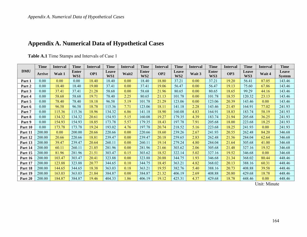
Appendix A. Numerical Data of Hypothetical Cases
Appendix A. Numerical Data of Hypothetical Cases Table A.1 Time Stamps and Intervals of Case 1
Time Interval Time Interval Time Interval Time Interval Time Interval Time Interval Time Interval Time DMU
Arrive Wait 1 Enter WS1 OP1 Leave
WS1 Wait2 Enter WS2 OP2 Leave
WS2 Wait 3 Enter WS3 OP3 Leave
WS3 Wait 4 Leave System
Part 1 0.00 0.00 0.00 18.40 18.40 0.00 18.40 18.80 37.21 0.00 37.21 19.20 56.41 87.05 143.46 Part 2 0.00 18.40 18.40 19.00 37.41 0.00 37.41 19.06 56.47 0.00 56.47 19.13 75.60 67.86 143.46 Part 3 0.00 37.41 37.41 21.28 58.68 0.00 58.68 21.96 80.65 0.00 80.65 18.65 99.29 44.16 143.46 Part 4 0.00 58.68 58.68 19.71 78.40 2.25 80.65 21.13 101.78 0.00 101.78 18.55 120.32 23.13 143.46 Part 5 0.00 78.40 78.40 18.18 96.58 5.19 101.78 21.29 123.06 0.00 123.06 20.39 143.46 0.00 143.46 Part 6 0.00 96.58 96.58 18.78 115.36 7.71 123.06 18.11 141.18 2.28 143.46 21.45 164.91 77.02 241.93 Part 7 0.00 115.36 115.36 18.96 134.32 6.86 141.18 18.90 160.08 4.83 164.91 18.83 183.74 58.19 241.93 Part 8 0.00 134.32 134.32 20.61 154.93 5.15 160.08 19.27 179.35 4.39 183.74 21.94 205.68 36.25 241.93 Part 9 0.00 154.93 154.93 18.85 173.78 5.57 179.35 18.43 197.78 7.91 205.68 18.00 223.68 18.25 241.93 Part 10 0.00 173.78 173.78 19.24 193.02 4.76 197.78 20.74 218.52 5.16 223.68 18.25 241.93 0.00 241.93 Part 11 200.00 0.00 200.00 20.66 220.66 0.00 220.66 18.60 239.26 2.67 241.93 20.55 262.48 84.20 346.68 Part 12 200.00 20.66 220.66 18.81 239.47 0.00 239.47 20.18 259.65 2.83 262.48 21.56 284.04 62.64 346.68 Part 13 200.00 39.47 239.47 20.64 260.11 0.00 260.11 19.14 279.24 4.80 284.04 21.64 305.68 41.00 346.68 Part 14 200.00 60.11 260.11 21.85 281.96 0.00 281.96 21.66 303.62 2.06 305.68 21.48 327.16 19.52 346.68 Part 15 200.00 81.96 281.96 21.51 303.47 0.15 303.62 18.52 322.14 5.02 327.16 19.52 346.68 0.00 346.68 Part 16 200.00 103.47 303.47 20.41 323.88 0.00 323.88 20.88 344.75 1.93 346.68 21.34 368.02 80.44 448.46 Part 17 200.00 123.88 323.88 20.77 344.65 0.10 344.75 18.45 363.21 4.82 368.02 20.13 388.16 60.31 448.46 Part 18 200.00 144.65 344.65 18.38 363.03 0.18 363.21 19.55 382.76 5.40 388.16 20.73 408.88 39.58 448.46 Part 19 200.00 163.03 363.03 21.84 384.87 0.00 384.87 21.32 406.19 2.69 408.88 20.80 429.68 18.78 448.46 Part 20 200.00 184.87 384.87 19.46 404.33 1.86 406.19 19.12 425.31 4.37 429.68 18.78 448.46 0.00 448.46
Unit: Minute
164
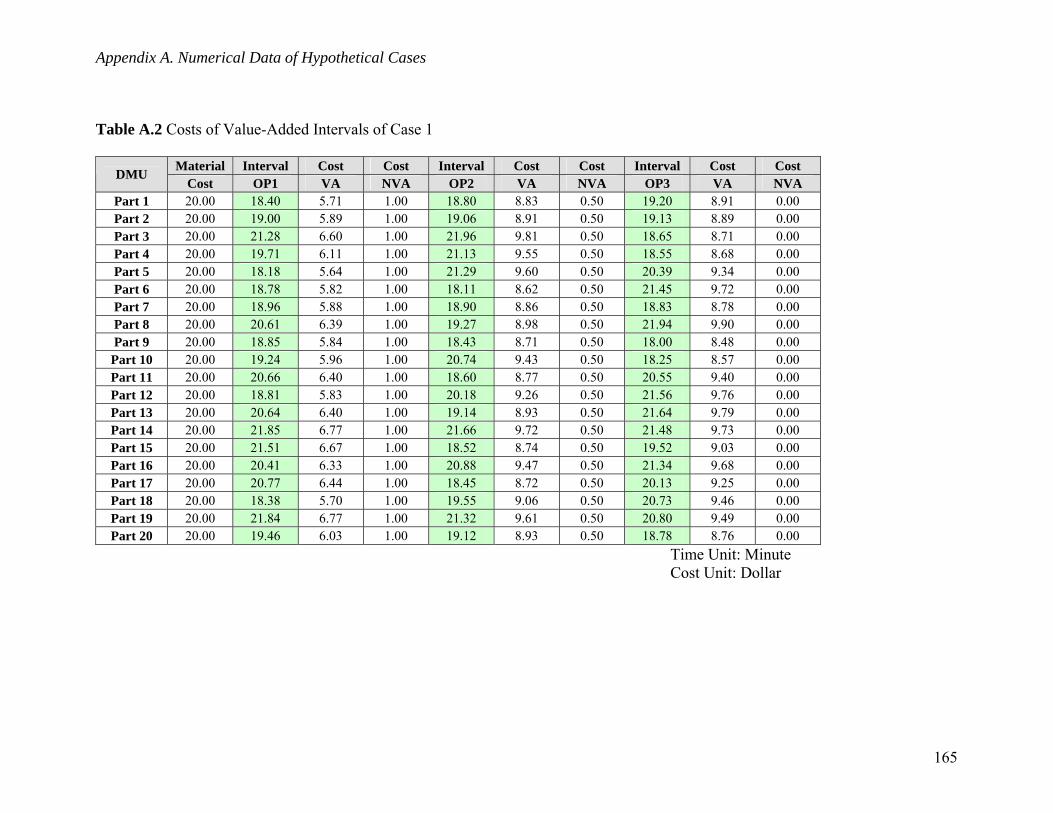
Appendix A. Numerical Data of Hypothetical Cases
Table A.2 Costs of Value-Added Intervals of Case 1
Material Interval Cost Cost Interval Cost Cost Interval Cost Cost DMU Cost OP1 VA NVA OP2 VA NVA OP3 VA NVA
Part 1 20.00 18.40 5.71 1.00 18.80 8.83 0.50 19.20 8.91 0.00 Part 2 20.00 19.00 5.89 1.00 19.06 8.91 0.50 19.13 8.89 0.00 Part 3 20.00 21.28 6.60 1.00 21.96 9.81 0.50 18.65 8.71 0.00 Part 4 20.00 19.71 6.11 1.00 21.13 9.55 0.50 18.55 8.68 0.00 Part 5 20.00 18.18 5.64 1.00 21.29 9.60 0.50 20.39 9.34 0.00 Part 6 20.00 18.78 5.82 1.00 18.11 8.62 0.50 21.45 9.72 0.00 Part 7 20.00 18.96 5.88 1.00 18.90 8.86 0.50 18.83 8.78 0.00 Part 8 20.00 20.61 6.39 1.00 19.27 8.98 0.50 21.94 9.90 0.00 Part 9 20.00 18.85 5.84 1.00 18.43 8.71 0.50 18.00 8.48 0.00 Part 10 20.00 19.24 5.96 1.00 20.74 9.43 0.50 18.25 8.57 0.00 Part 11 20.00 20.66 6.40 1.00 18.60 8.77 0.50 20.55 9.40 0.00 Part 12 20.00 18.81 5.83 1.00 20.18 9.26 0.50 21.56 9.76 0.00 Part 13 20.00 20.64 6.40 1.00 19.14 8.93 0.50 21.64 9.79 0.00 Part 14 20.00 21.85 6.77 1.00 21.66 9.72 0.50 21.48 9.73 0.00 Part 15 20.00 21.51 6.67 1.00 18.52 8.74 0.50 19.52 9.03 0.00 Part 16 20.00 20.41 6.33 1.00 20.88 9.47 0.50 21.34 9.68 0.00 Part 17 20.00 20.77 6.44 1.00 18.45 8.72 0.50 20.13 9.25 0.00 Part 18 20.00 18.38 5.70 1.00 19.55 9.06 0.50 20.73 9.46 0.00 Part 19 20.00 21.84 6.77 1.00 21.32 9.61 0.50 20.80 9.49 0.00 Part 20 20.00 19.46 6.03 1.00 19.12 8.93 0.50 18.78 8.76 0.00
Time Unit: Minute Cost Unit: Dollar
165

Appendix A. Numerical Data of Hypothetical Cases
Table A.3 Costs of Non-Value-Added Intervals of Case 1
Interval Cost Interval Cost Interval Cost Interval Cost DMU Wait 1 NVA Wait2 NVA Wait 3 NVA Wait 4 NVA
Part 1 0.00 0.00 0.00 0.00 0.00 0.00 87.05 0.87 Part 2 18.40 0.18 0.00 0.00 0.00 0.00 67.86 0.68 Part 3 37.41 0.37 0.00 0.00 0.00 0.00 44.16 0.44 Part 4 58.68 0.59 2.25 0.02 0.00 0.00 23.13 0.23 Part 5 78.40 0.78 5.19 0.05 0.00 0.00 0.00 0.00 Part 6 96.58 0.97 7.71 0.08 2.28 0.02 77.02 0.77 Part 7 115.36 1.15 6.86 0.07 4.83 0.05 58.19 0.58 Part 8 134.32 1.34 5.15 0.05 4.39 0.04 36.25 0.36 Part 9 154.93 1.55 5.57 0.06 7.91 0.08 18.25 0.18
Part 10 173.78 1.74 4.76 0.05 5.16 0.05 0.00 0.00 Part 11 0.00 0.00 0.00 0.00 2.67 0.03 84.20 0.84 Part 12 20.66 0.21 0.00 0.00 2.83 0.03 62.64 0.63 Part 13 39.47 0.39 0.00 0.00 4.80 0.05 41.00 0.41 Part 14 60.11 0.60 0.00 0.00 2.06 0.02 19.52 0.20 Part 15 81.96 0.82 0.15 0.00 5.02 0.05 0.00 0.00 Part 16 103.47 1.03 0.00 0.00 1.93 0.02 80.44 0.80 Part 17 123.88 1.24 0.10 0.00 4.82 0.05 60.31 0.60 Part 18 144.65 1.45 0.18 0.00 5.40 0.05 39.58 0.40 Part 19 163.03 1.63 0.00 0.00 2.69 0.03 18.78 0.19 Part 20 184.87 1.85 1.86 0.02 4.37 0.04 0.00 0.00
Time Unit: Minute Cost Unit: Dollar
166
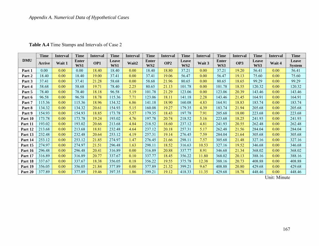
Appendix A. Numerical Data of Hypothetical Cases
Table A.4 Time Stamps and Intervals of Case 2
Time Interval Time Interval Time Interval Time Interval Time Interval Time Interval Time Interval Time DMU
Arrive Wait 1 Enter WS1 OP1 Leave
WS1 Wait2 Enter WS2 OP2 Leave
WS2 Wait 3 Enter WS3 OP3 Leave
WS3 Wait 4 Leave System
Part 1 0.00 0.00 0.00 18.40 18.40 0.00 18.40 18.80 37.21 0.00 37.21 19.20 56.41 0.00 56.41 Part 2 18.40 0.00 18.40 19.00 37.41 0.00 37.41 19.06 56.47 0.00 56.47 19.13 75.60 0.00 75.60 Part 3 37.41 0.00 37.41 21.28 58.68 0.00 58.68 21.96 80.65 0.00 80.65 18.65 99.29 0.00 99.29 Part 4 58.68 0.00 58.68 19.71 78.40 2.25 80.65 21.13 101.78 0.00 101.78 18.55 120.32 0.00 120.32 Part 5 78.40 0.00 78.40 18.18 96.58 5.19 101.78 21.29 123.06 0.00 123.06 20.39 143.46 0.00 143.46 Part 6 96.58 0.00 96.58 18.78 115.36 7.71 123.06 18.11 141.18 2.28 143.46 21.45 164.91 0.00 164.91 Part 7 115.36 0.00 115.36 18.96 134.32 6.86 141.18 18.90 160.08 4.83 164.91 18.83 183.74 0.00 183.74 Part 8 134.32 0.00 134.32 20.61 154.93 5.15 160.08 19.27 179.35 4.39 183.74 21.94 205.68 0.00 205.68 Part 9 154.93 0.00 154.93 18.85 173.78 5.57 179.35 18.43 197.78 7.91 205.68 18.00 223.68 0.00 223.68 Part 10 173.78 0.00 173.78 19.24 193.02 4.76 197.78 20.74 218.52 5.16 223.68 18.25 241.93 0.00 241.93 Part 11 193.02 0.00 193.02 20.66 213.68 4.84 218.52 18.60 237.12 4.81 241.93 20.55 262.48 0.00 262.48 Part 12 213.68 0.00 213.68 18.81 232.48 4.64 237.12 20.18 257.31 5.17 262.48 21.56 284.04 0.00 284.04 Part 13 232.48 0.00 232.48 20.64 253.12 4.19 257.31 19.14 276.45 7.59 284.04 21.64 305.68 0.00 305.68 Part 14 253.12 0.00 253.12 21.85 274.97 1.47 276.45 21.66 298.11 7.57 305.68 21.48 327.16 0.00 327.16 Part 15 274.97 0.00 274.97 21.51 296.48 1.63 298.11 18.52 316.63 10.53 327.16 19.52 346.68 0.00 346.68 Part 16 296.48 0.00 296.48 20.41 316.89 0.00 316.89 20.88 337.77 8.91 346.68 21.34 368.02 0.00 368.02 Part 17 316.89 0.00 316.89 20.77 337.67 0.10 337.77 18.45 356.22 11.80 368.02 20.13 388.16 0.00 388.16 Part 18 337.67 0.00 337.67 18.38 356.05 0.18 356.22 19.55 375.78 12.38 388.16 20.73 408.88 0.00 408.88 Part 19 356.05 0.00 356.05 21.84 377.89 0.00 377.89 21.32 399.21 9.67 408.88 20.80 429.68 0.00 429.68 Part 20 377.89 0.00 377.89 19.46 397.35 1.86 399.21 19.12 418.33 11.35 429.68 18.78 448.46 0.00 448.46
Unit: Minute
167

Appendix A. Numerical Data of Hypothetical Cases
Table A.5 Costs of Value-Added Intervals of Case 2
Material Interval Cost Cost Interval Cost Cost Interval Cost Cost DMU Cost OP1 VA NVA OP2 VA NVA OP3 VA NVA
Part 1 20.00 18.40 5.71 1.00 18.80 8.83 0.50 19.20 8.91 0.00 Part 2 20.00 19.00 5.89 1.00 19.06 8.91 0.50 19.13 8.89 0.00 Part 3 20.00 21.28 6.60 1.00 21.96 9.81 0.50 18.65 8.71 0.00 Part 4 20.00 19.71 6.11 1.00 21.13 9.55 0.50 18.55 8.68 0.00 Part 5 20.00 18.18 5.64 1.00 21.29 9.60 0.50 20.39 9.34 0.00 Part 6 20.00 18.78 5.82 1.00 18.11 8.62 0.50 21.45 9.72 0.00 Part 7 20.00 18.96 5.88 1.00 18.90 8.86 0.50 18.83 8.78 0.00 Part 8 20.00 20.61 6.39 1.00 19.27 8.98 0.50 21.94 9.90 0.00 Part 9 20.00 18.85 5.84 1.00 18.43 8.71 0.50 18.00 8.48 0.00 Part 10 20.00 19.24 5.96 1.00 20.74 9.43 0.50 18.25 8.57 0.00 Part 11 20.00 20.66 6.40 1.00 18.60 8.77 0.50 20.55 9.40 0.00 Part 12 20.00 18.81 5.83 1.00 20.18 9.26 0.50 21.56 9.76 0.00 Part 13 20.00 20.64 6.40 1.00 19.14 8.93 0.50 21.64 9.79 0.00 Part 14 20.00 21.85 6.77 1.00 21.66 9.72 0.50 21.48 9.73 0.00 Part 15 20.00 21.51 6.67 1.00 18.52 8.74 0.50 19.52 9.03 0.00 Part 16 20.00 20.41 6.33 1.00 20.88 9.47 0.50 21.34 9.68 0.00 Part 17 20.00 20.77 6.44 1.00 18.45 8.72 0.50 20.13 9.25 0.00 Part 18 20.00 18.38 5.70 1.00 19.55 9.06 0.50 20.73 9.46 0.00 Part 19 20.00 21.84 6.77 1.00 21.32 9.61 0.50 20.80 9.49 0.00 Part 20 20.00 19.46 6.03 1.00 19.12 8.93 0.50 18.78 8.76 0.00
Time Unit: Minute Cost Unit: Dollar
168

Appendix A. Numerical Data of Hypothetical Cases
Table A.6 Costs of Non-Value-Added Intervals of Case 2
Interval Cost Interval Cost Interval Cost Interval Cost DMU Wait 1 NVA Wait2 NVA Wait 3 NVA Wait 4 NVA
Part 1 0.00 0.00 0.00 0.00 0.00 0.00 0.00 0.00 Part 2 0.00 0.00 0.00 0.00 0.00 0.00 0.00 0.00 Part 3 0.00 0.00 0.00 0.00 0.00 0.00 0.00 0.00 Part 4 0.00 0.00 2.25 0.02 0.00 0.00 0.00 0.00 Part 5 0.00 0.00 5.19 0.05 0.00 0.00 0.00 0.00 Part 6 0.00 0.00 7.71 0.08 2.28 0.02 0.00 0.00 Part 7 0.00 0.00 6.86 0.07 4.83 0.05 0.00 0.00 Part 8 0.00 0.00 5.15 0.05 4.39 0.04 0.00 0.00 Part 9 0.00 0.00 5.57 0.06 7.91 0.08 0.00 0.00
Part 10 0.00 0.00 4.76 0.05 5.16 0.05 0.00 0.00 Part 11 0.00 0.00 4.84 0.05 4.81 0.05 0.00 0.00 Part 12 0.00 0.00 4.64 0.05 5.17 0.05 0.00 0.00 Part 13 0.00 0.00 4.19 0.04 7.59 0.08 0.00 0.00 Part 14 0.00 0.00 1.47 0.01 7.57 0.08 0.00 0.00 Part 15 0.00 0.00 1.63 0.02 10.53 0.11 0.00 0.00 Part 16 0.00 0.00 0.00 0.00 8.91 0.09 0.00 0.00 Part 17 0.00 0.00 0.10 0.00 11.80 0.12 0.00 0.00 Part 18 0.00 0.00 0.18 0.00 12.38 0.12 0.00 0.00 Part 19 0.00 0.00 0.00 0.00 9.67 0.10 0.00 0.00 Part 20 0.00 0.00 1.86 0.02 11.35 0.11 0.00 0.00
Time Unit: Minute Cost Unit: Dollar
169
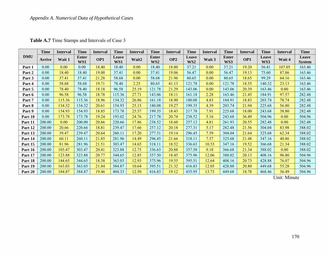
Appendix A. Numerical Data of Hypothetical Cases
Table A.7 Time Stamps and Intervals of Case 3
Time Interval Time Interval Time Interval Time Interval Time Interval Time Interval Time Interval Time DMU
Arrive Wait 1 Enter WS1 OP1 Leave
WS1 Wait2 Enter WS2 OP2 Leave
WS2 Wait 3 Enter WS3 OP3 Leave
WS3 Wait 4 Leave System
Part 1 0.00 0.00 0.00 18.40 18.40 0.00 18.40 18.80 37.21 0.00 37.21 19.20 56.41 107.05 163.46 Part 2 0.00 18.40 18.40 19.00 37.41 0.00 37.41 19.06 56.47 0.00 56.47 19.13 75.60 87.86 163.46 Part 3 0.00 37.41 37.41 21.28 58.68 0.00 58.68 21.96 80.65 0.00 80.65 18.65 99.29 64.16 163.46 Part 4 0.00 58.68 58.68 19.71 78.40 2.25 80.65 41.13 121.78 0.00 121.78 18.55 140.32 23.13 163.46 Part 5 0.00 78.40 78.40 18.18 96.58 25.19 121.78 21.29 143.06 0.00 143.06 20.39 163.46 0.00 163.46 Part 6 0.00 96.58 96.58 18.78 115.36 27.71 143.06 18.11 161.18 2.28 163.46 21.45 184.91 97.57 282.48 Part 7 0.00 115.36 115.36 18.96 134.32 26.86 161.18 18.90 180.08 4.83 184.91 18.83 203.74 78.74 282.48 Part 8 0.00 134.32 134.32 20.61 154.93 25.15 180.08 19.27 199.35 4.39 203.74 21.94 225.68 56.80 282.48 Part 9 0.00 154.93 154.93 18.85 173.78 25.57 199.35 18.43 217.78 7.91 225.68 18.00 243.68 38.80 282.48 Part 10 0.00 173.78 173.78 19.24 193.02 24.76 217.78 20.74 238.52 5.16 243.68 36.49 504.96 0.00 504.96 Part 11 200.00 0.00 200.00 20.66 220.66 17.86 238.52 18.60 257.12 4.81 261.93 20.55 282.48 0.00 282.48 Part 12 200.00 20.66 220.66 18.81 239.47 17.66 257.12 20.18 277.31 5.17 282.48 21.56 304.04 83.98 388.02 Part 13 200.00 39.47 239.47 20.64 260.11 17.20 277.31 19.14 296.45 7.59 304.04 21.64 325.68 62.34 388.02 Part 14 200.00 60.11 260.11 21.85 281.96 14.49 296.45 21.66 318.11 7.57 325.68 21.48 347.16 40.86 388.02 Part 15 200.00 81.96 281.96 21.51 303.47 14.65 318.11 18.52 336.63 10.53 347.16 19.52 366.68 21.34 388.02 Part 16 200.00 103.47 303.47 20.41 323.88 12.75 336.63 20.88 357.50 9.18 366.68 21.34 388.02 0.00 388.02 Part 17 200.00 123.88 323.88 20.77 344.65 12.85 357.50 18.45 375.96 12.06 388.02 20.13 408.16 96.80 504.96 Part 18 200.00 144.65 344.65 18.38 363.03 12.93 375.96 19.55 395.51 12.64 408.16 20.73 428.88 76.07 504.96 Part 19 200.00 163.03 363.03 21.84 384.87 10.64 395.51 21.32 416.83 12.05 428.88 20.80 449.68 55.28 504.96 Part 20 200.00 184.87 384.87 19.46 404.33 12.50 416.83 19.12 435.95 13.73 449.68 18.78 468.46 36.49 504.96
Unit: Minute
170

Appendix A. Numerical Data of Hypothetical Cases
Table A.8 Costs of Value-Added Intervals of Case 3
Material Interval Cost Cost Interval Cost Cost Interval Cost Cost DMU Cost OP1 VA NVA OP2 VA NVA OP3 VA NVA
Part 1 20.00 18.40 5.71 1.00 18.80 8.83 0.50 19.20 8.91 0.00 Part 2 20.00 19.00 5.89 1.00 19.06 8.91 0.50 19.13 8.89 0.00 Part 3 20.00 21.28 6.60 1.00 21.96 9.81 0.50 18.65 8.71 0.00 Part 4 20.00 19.71 6.11 1.00 41.13 15.75 0.50 18.55 8.68 0.00 Part 5 20.00 18.18 5.64 1.00 21.29 9.60 0.50 20.39 9.34 0.00 Part 6 20.00 18.78 5.82 1.00 18.11 8.62 0.50 21.45 9.72 0.00 Part 7 20.00 18.96 5.88 1.00 18.90 8.86 0.50 18.83 8.78 0.00 Part 8 20.00 20.61 6.39 1.00 19.27 8.98 0.50 21.94 9.90 0.00 Part 9 20.00 18.85 5.84 1.00 18.43 8.71 0.50 18.00 8.48 0.00 Part 10 20.00 19.24 5.96 1.00 20.74 9.43 0.50 36.49 15.14 0.00 Part 11 20.00 20.66 6.40 1.00 18.60 8.77 0.50 20.55 9.40 0.00 Part 12 20.00 18.81 5.83 1.00 20.18 9.26 0.50 21.56 9.76 0.00 Part 13 20.00 20.64 6.40 1.00 19.14 8.93 0.50 21.64 9.79 0.00 Part 14 20.00 21.85 6.77 1.00 21.66 9.72 0.50 21.48 9.73 0.00 Part 15 20.00 21.51 6.67 1.00 18.52 8.74 0.50 19.52 9.03 0.00 Part 16 20.00 20.41 6.33 1.00 20.88 9.47 0.50 21.34 9.68 0.00 Part 17 20.00 20.77 6.44 1.00 18.45 8.72 0.50 20.13 9.25 0.00 Part 18 20.00 18.38 5.70 1.00 19.55 9.06 0.50 20.73 9.46 0.00 Part 19 20.00 21.84 6.77 1.00 21.32 9.61 0.50 20.80 9.49 0.00 Part 20 20.00 19.46 6.03 1.00 19.12 8.93 0.50 18.78 8.76 0.00
Time Unit: Minute Cost Unit: Dollar
171
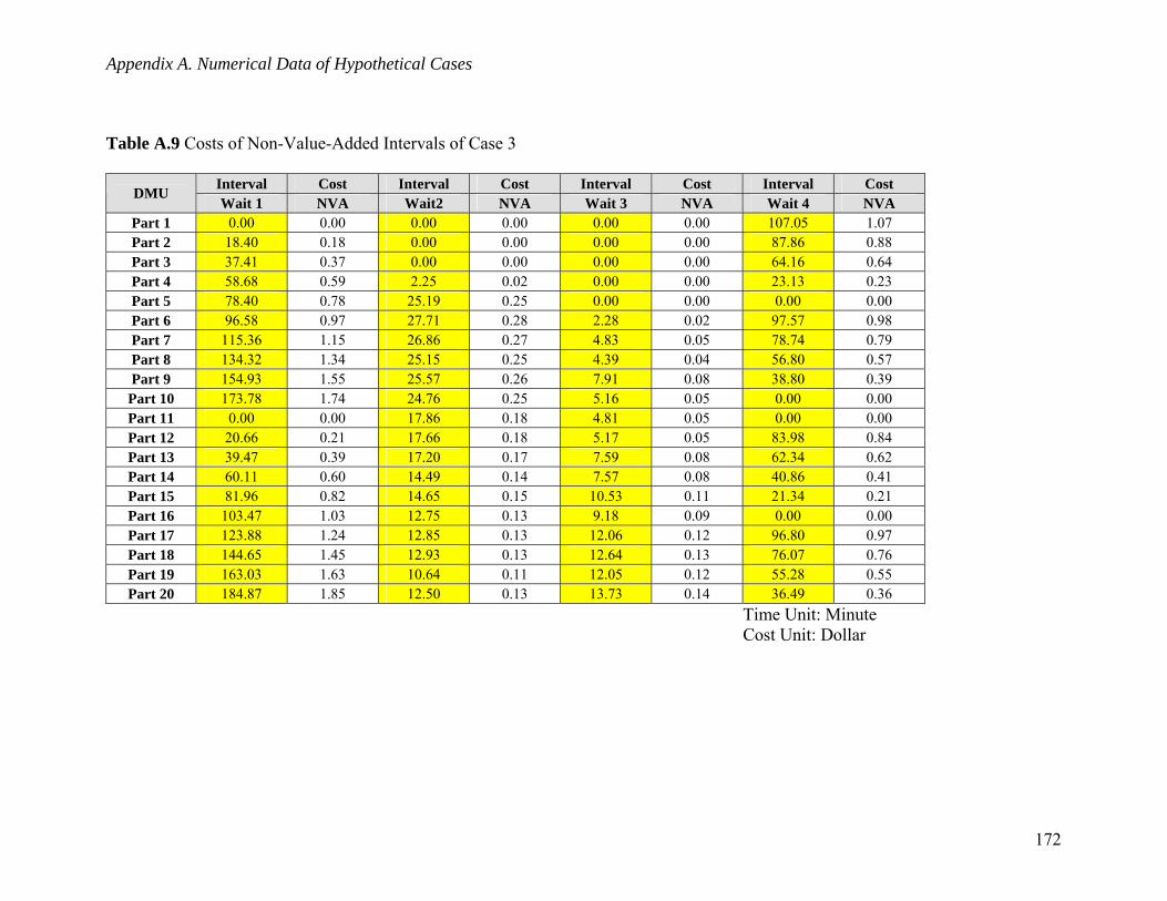
Appendix A. Numerical Data of Hypothetical Cases
Table A.9 Costs of Non-Value-Added Intervals of Case 3
Interval Cost Interval Cost Interval Cost Interval Cost DMU Wait 1 NVA Wait2 NVA Wait 3 NVA Wait 4 NVA
Part 1 0.00 0.00 0.00 0.00 0.00 0.00 107.05 1.07 Part 2 18.40 0.18 0.00 0.00 0.00 0.00 87.86 0.88 Part 3 37.41 0.37 0.00 0.00 0.00 0.00 64.16 0.64 Part 4 58.68 0.59 2.25 0.02 0.00 0.00 23.13 0.23 Part 5 78.40 0.78 25.19 0.25 0.00 0.00 0.00 0.00 Part 6 96.58 0.97 27.71 0.28 2.28 0.02 97.57 0.98 Part 7 115.36 1.15 26.86 0.27 4.83 0.05 78.74 0.79 Part 8 134.32 1.34 25.15 0.25 4.39 0.04 56.80 0.57 Part 9 154.93 1.55 25.57 0.26 7.91 0.08 38.80 0.39
Part 10 173.78 1.74 24.76 0.25 5.16 0.05 0.00 0.00 Part 11 0.00 0.00 17.86 0.18 4.81 0.05 0.00 0.00 Part 12 20.66 0.21 17.66 0.18 5.17 0.05 83.98 0.84 Part 13 39.47 0.39 17.20 0.17 7.59 0.08 62.34 0.62 Part 14 60.11 0.60 14.49 0.14 7.57 0.08 40.86 0.41 Part 15 81.96 0.82 14.65 0.15 10.53 0.11 21.34 0.21 Part 16 103.47 1.03 12.75 0.13 9.18 0.09 0.00 0.00 Part 17 123.88 1.24 12.85 0.13 12.06 0.12 96.80 0.97 Part 18 144.65 1.45 12.93 0.13 12.64 0.13 76.07 0.76 Part 19 163.03 1.63 10.64 0.11 12.05 0.12 55.28 0.55 Part 20 184.87 1.85 12.50 0.13 13.73 0.14 36.49 0.36
Time Unit: Minute Cost Unit: Dollar
172
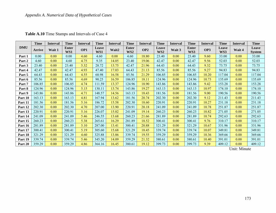
Appendix A. Numerical Data of Hypothetical Cases
Table A.10 Time Stamps and Intervals of Case 4
Time Interval Time Interval Time Interval Time Interval Time Interval Time Interval Time Interval Time DMU
Arrive Wait 1 Enter WS1 OP1 Leave
WS1 Wait2 Enter WS2 OP2 Leave
WS2 Wait 3 Enter WS3 OP3 Leave
WS3 Wait 4 Leave System
Part 1 0.00 0.00 0.00 4.60 4.60 0.00 4.60 18.80 23.40 0.00 23.40 9.60 33.00 0.00 33.00 Part 2 4.60 0.00 4.60 4.75 9.35 14.05 23.40 19.06 42.47 0.00 42.47 9.56 52.03 0.00 52.03 Part 3 23.40 0.00 23.40 5.32 28.72 13.75 42.47 21.96 64.43 0.00 64.43 9.32 73.75 0.00 73.75 Part 4 42.47 0.00 42.47 4.93 47.40 17.03 64.43 21.13 85.56 0.00 85.56 9.27 94.83 0.00 94.83 Part 5 64.43 0.00 64.43 4.55 68.98 16.58 85.56 21.29 106.85 0.00 106.85 10.20 117.04 0.00 117.04 Part 6 85.56 0.00 85.56 4.69 90.25 16.59 106.85 18.11 124.96 0.00 124.96 10.73 135.69 0.00 135.69 Part 7 106.85 0.00 106.85 4.74 111.59 13.37 124.96 18.90 143.86 0.00 143.86 9.42 153.28 0.00 153.28 Part 8 124.96 0.00 124.96 5.15 130.11 13.74 143.86 19.27 163.13 0.00 163.13 10.97 174.10 0.00 174.10 Part 9 143.86 0.00 143.86 4.71 148.57 14.56 163.13 18.43 181.56 0.00 181.56 9.00 190.56 0.00 190.56 Part 10 163.13 0.00 163.13 4.81 167.94 13.62 181.56 20.74 202.30 0.00 202.30 9.12 211.43 0.00 211.43 Part 11 181.56 0.00 181.56 5.16 186.72 15.58 202.30 18.60 220.91 0.00 220.91 10.27 231.18 0.00 231.18 Part 12 202.30 0.00 202.30 4.70 207.00 13.90 220.91 20.18 241.09 0.00 241.09 10.78 251.87 0.00 251.87 Part 13 220.91 0.00 220.91 5.16 226.07 15.02 241.09 19.14 260.23 0.00 260.23 10.82 271.05 0.00 271.05 Part 14 241.09 0.00 241.09 5.46 246.55 13.68 260.23 21.66 281.89 0.00 281.89 10.74 292.63 0.00 292.63 Part 15 260.23 0.00 260.23 5.38 265.61 16.29 281.89 18.52 300.41 0.00 300.41 9.76 310.17 0.00 310.17 Part 16 281.89 0.00 281.89 5.10 287.00 13.41 300.41 20.88 321.29 0.00 321.29 10.67 331.96 0.00 331.96 Part 17 300.41 0.00 300.41 5.19 305.60 15.68 321.29 18.45 339.74 0.00 339.74 10.07 349.81 0.00 349.81 Part 18 321.29 0.00 321.29 4.60 325.88 13.86 339.74 19.55 359.29 0.00 359.29 10.36 369.66 0.00 369.66 Part 19 339.74 0.00 339.74 5.46 345.20 14.09 359.29 21.32 380.61 0.00 380.61 10.40 391.01 0.00 391.01 Part 20 359.29 0.00 359.29 4.86 364.16 16.45 380.61 19.12 399.73 0.00 399.73 9.39 409.12 0.00 409.12
Unit: Minute
173

Appendix A. Numerical Data of Hypothetical Cases
Table A.11 Costs of Value-Added Intervals of Case 4
Material Interval Cost Cost Interval Cost Cost Interval Cost Cost DMU Cost OP1 VA NVA OP2 VA NVA OP3 VA NVA
Part 1 20.00 4.60 1.43 1.00 18.80 8.83 0.50 9.60 5.46 0.00 Part 2 20.00 4.75 1.47 1.00 19.06 8.91 0.50 9.56 5.44 0.00 Part 3 20.00 5.32 1.65 1.00 21.96 9.81 0.50 9.32 5.36 0.00 Part 4 20.00 4.93 1.53 1.00 21.13 9.55 0.50 9.27 5.34 0.00 Part 5 20.00 4.55 1.41 1.00 21.29 9.60 0.50 10.20 5.67 0.00 Part 6 20.00 4.69 1.46 1.00 18.11 8.62 0.50 10.73 5.86 0.00 Part 7 20.00 4.74 1.47 1.00 18.90 8.86 0.50 9.42 5.39 0.00 Part 8 20.00 5.15 1.60 1.00 19.27 8.98 0.50 10.97 5.95 0.00 Part 9 20.00 4.71 1.46 1.00 18.43 8.71 0.50 9.00 5.24 0.00 Part 10 20.00 4.81 1.49 1.00 20.74 9.43 0.50 9.12 5.28 0.00 Part 11 20.00 5.16 1.60 1.00 18.60 8.77 0.50 10.27 5.70 0.00 Part 12 20.00 4.70 1.46 1.00 20.18 9.26 0.50 10.78 5.88 0.00 Part 13 20.00 5.16 1.60 1.00 19.14 8.93 0.50 10.82 5.89 0.00 Part 14 20.00 5.46 1.69 1.00 21.66 9.72 0.50 10.74 5.87 0.00 Part 15 20.00 5.38 1.67 1.00 18.52 8.74 0.50 9.76 5.51 0.00 Part 16 20.00 5.10 1.58 1.00 20.88 9.47 0.50 10.67 5.84 0.00 Part 17 20.00 5.19 1.61 1.00 18.45 8.72 0.50 10.07 5.62 0.00 Part 18 20.00 4.60 1.42 1.00 19.55 9.06 0.50 10.36 5.73 0.00 Part 19 20.00 5.46 1.69 1.00 21.32 9.61 0.50 10.40 5.74 0.00 Part 20 20.00 4.86 1.51 1.00 19.12 8.93 0.50 9.39 5.38 0.00
Time Unit: Minute Cost Unit: Dollar
174

Appendix A. Numerical Data of Hypothetical Cases
Table A.12 Costs of Non-Value-Added Intervals of Case 4
Interval Cost Interval Cost Interval Cost Interval Cost DMU Wait 1 NVA Wait2 NVA Wait 3 NVA Wait 4 NVA
Part 1 0.00 0.00 0.00 0.00 0.00 0.00 0.00 0.00 Part 2 0.00 0.00 14.05 0.14 0.00 0.00 0.00 0.00 Part 3 0.00 0.00 13.75 0.14 0.00 0.00 0.00 0.00 Part 4 0.00 0.00 17.03 0.17 0.00 0.00 0.00 0.00 Part 5 0.00 0.00 16.58 0.17 0.00 0.00 0.00 0.00 Part 6 0.00 0.00 16.59 0.17 0.00 0.00 0.00 0.00 Part 7 0.00 0.00 13.37 0.13 0.00 0.00 0.00 0.00 Part 8 0.00 0.00 13.74 0.14 0.00 0.00 0.00 0.00 Part 9 0.00 0.00 14.56 0.15 0.00 0.00 0.00 0.00
Part 10 0.00 0.00 13.62 0.14 0.00 0.00 0.00 0.00 Part 11 0.00 0.00 15.58 0.16 0.00 0.00 0.00 0.00 Part 12 0.00 0.00 13.90 0.14 0.00 0.00 0.00 0.00 Part 13 0.00 0.00 15.02 0.15 0.00 0.00 0.00 0.00 Part 14 0.00 0.00 13.68 0.14 0.00 0.00 0.00 0.00 Part 15 0.00 0.00 16.29 0.16 0.00 0.00 0.00 0.00 Part 16 0.00 0.00 13.41 0.13 0.00 0.00 0.00 0.00 Part 17 0.00 0.00 15.68 0.16 0.00 0.00 0.00 0.00 Part 18 0.00 0.00 13.86 0.14 0.00 0.00 0.00 0.00 Part 19 0.00 0.00 14.09 0.14 0.00 0.00 0.00 0.00 Part 20 0.00 0.00 16.45 0.16 0.00 0.00 0.00 0.00
Time Unit: Minute Cost Unit: Dollar
175

Appendix A. Numerical Data of Hypothetical Cases
Table A.13 Time Stamps and Intervals of Case 5: Day 1
Time Interval Time Interval Time Interval Time Interval Time Interval Time Interval Time Interval Time DMU
Arrive Wait 1 Enter WS1 OP1 Leave
WS1 Wait2 Enter WS2 OP2 Leave
WS2 Wait 3 Enter WS3 OP3 Leave
WS3 Wait 4 Leave System
Part 1 0.00 0.00 0.00 18.05 18.05 0.00 18.05 18.09 36.14 0.00 36.14 18.14 54.28 383.45 437.73 Part 2 18.05 0.00 18.05 20.58 38.63 0.00 38.63 18.22 56.85 0.00 56.85 19.86 76.71 361.03 437.73 Part 3 38.63 0.00 38.63 18.65 57.28 0.00 57.28 20.70 77.98 0.00 77.98 18.76 96.74 340.99 437.73 Part 4 57.28 0.00 57.28 20.35 77.63 0.35 77.98 18.40 96.39 0.36 96.74 20.46 117.20 320.53 437.73 Part 5 77.63 0.00 77.63 18.84 96.47 0.00 96.47 18.60 115.07 2.13 117.20 18.36 135.56 302.17 437.73 Part 6 96.47 0.00 96.47 20.65 117.12 0.00 117.12 21.85 138.97 0.00 138.97 19.06 158.03 279.70 437.73 Part 7 117.12 0.00 117.12 21.19 138.31 0.66 138.97 19.37 158.34 0.00 158.34 21.54 179.88 257.86 437.73 Part 8 138.31 0.00 138.31 18.28 156.59 1.75 158.34 18.61 176.95 2.93 179.88 18.95 198.83 238.91 437.73 Part 9 156.59 0.00 156.59 19.00 175.59 1.36 176.95 18.73 195.68 3.14 198.83 18.46 217.29 220.44 437.73 Part 10 175.59 0.00 175.59 18.43 194.02 1.66 195.68 19.13 214.81 2.48 217.29 19.82 237.11 200.62 437.73 Part 11 194.02 0.00 194.02 20.71 214.74 0.08 214.81 18.71 233.52 3.59 237.11 20.70 257.81 179.92 437.73 Part 12 214.74 0.00 214.74 18.03 232.76 0.75 233.52 18.62 252.14 5.67 257.81 19.22 277.03 160.70 437.73 Part 13 232.76 0.00 232.76 18.12 250.88 1.26 252.14 18.09 270.24 6.80 277.03 18.07 295.11 142.63 437.73 Part 14 250.88 0.00 250.88 18.23 269.11 1.12 270.24 18.43 288.67 6.44 295.11 18.63 313.74 124.00 437.73 Part 15 269.11 0.00 269.11 21.21 290.32 0.00 290.32 21.91 312.23 1.51 313.74 18.61 332.34 105.39 437.73 Part 16 290.32 0.00 290.32 18.87 309.19 3.03 312.23 21.80 334.02 0.00 334.02 20.73 354.75 82.98 437.73 Part 17 309.19 0.00 309.19 18.47 327.66 6.36 334.02 21.85 355.87 0.00 355.87 21.23 377.10 60.63 437.73 Part 18 327.66 0.00 327.66 18.87 346.53 9.35 355.87 20.53 376.40 0.70 377.10 18.18 395.28 42.45 437.73 Part 19 346.53 0.00 346.53 19.17 365.70 10.70 376.40 19.98 396.38 0.00 396.38 20.78 417.16 20.57 437.73 Part 20 365.70 0.00 365.70 18.55 384.25 12.13 396.38 21.30 417.68 0.00 417.68 20.06 437.73 0.00 437.73
Unit: Minute
176
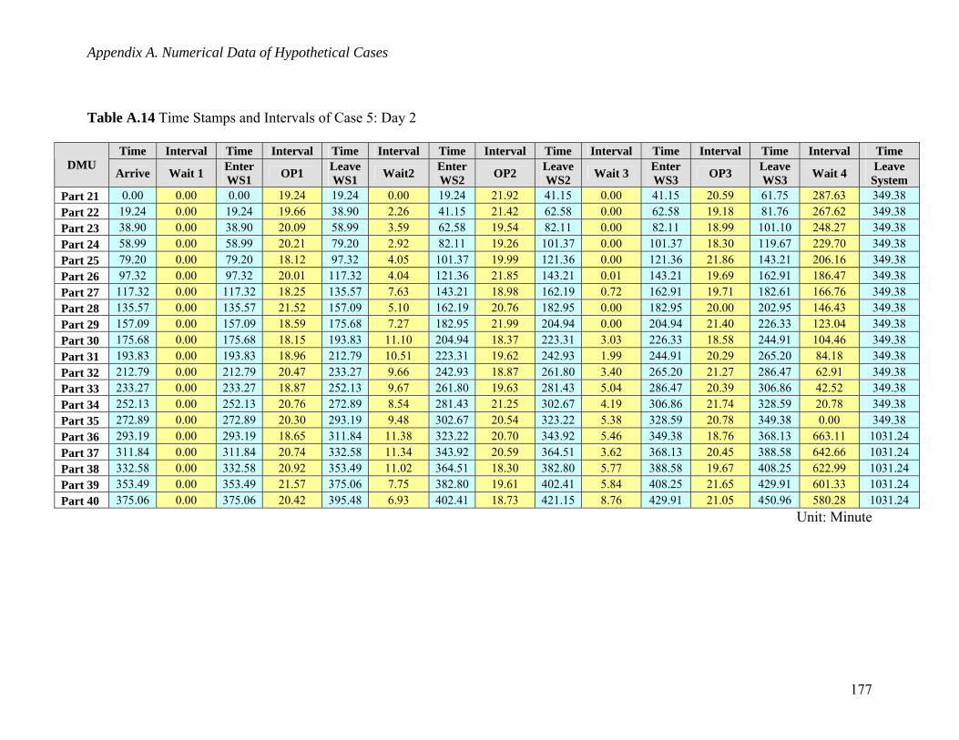
Appendix A. Numerical Data of Hypothetical Cases
Table A.14 Time Stamps and Intervals of Case 5: Day 2
Time Interval Time Interval Time Interval Time Interval Time Interval Time Interval Time Interval Time DMU
Arrive Wait 1 Enter WS1 OP1 Leave
WS1 Wait2 Enter WS2 OP2 Leave
WS2 Wait 3 Enter WS3 OP3 Leave
WS3 Wait 4 Leave System
Part 21 0.00 0.00 0.00 19.24 19.24 0.00 19.24 21.92 41.15 0.00 41.15 20.59 61.75 287.63 349.38 Part 22 19.24 0.00 19.24 19.66 38.90 2.26 41.15 21.42 62.58 0.00 62.58 19.18 81.76 267.62 349.38 Part 23 38.90 0.00 38.90 20.09 58.99 3.59 62.58 19.54 82.11 0.00 82.11 18.99 101.10 248.27 349.38 Part 24 58.99 0.00 58.99 20.21 79.20 2.92 82.11 19.26 101.37 0.00 101.37 18.30 119.67 229.70 349.38 Part 25 79.20 0.00 79.20 18.12 97.32 4.05 101.37 19.99 121.36 0.00 121.36 21.86 143.21 206.16 349.38 Part 26 97.32 0.00 97.32 20.01 117.32 4.04 121.36 21.85 143.21 0.01 143.21 19.69 162.91 186.47 349.38 Part 27 117.32 0.00 117.32 18.25 135.57 7.63 143.21 18.98 162.19 0.72 162.91 19.71 182.61 166.76 349.38 Part 28 135.57 0.00 135.57 21.52 157.09 5.10 162.19 20.76 182.95 0.00 182.95 20.00 202.95 146.43 349.38 Part 29 157.09 0.00 157.09 18.59 175.68 7.27 182.95 21.99 204.94 0.00 204.94 21.40 226.33 123.04 349.38 Part 30 175.68 0.00 175.68 18.15 193.83 11.10 204.94 18.37 223.31 3.03 226.33 18.58 244.91 104.46 349.38 Part 31 193.83 0.00 193.83 18.96 212.79 10.51 223.31 19.62 242.93 1.99 244.91 20.29 265.20 84.18 349.38 Part 32 212.79 0.00 212.79 20.47 233.27 9.66 242.93 18.87 261.80 3.40 265.20 21.27 286.47 62.91 349.38 Part 33 233.27 0.00 233.27 18.87 252.13 9.67 261.80 19.63 281.43 5.04 286.47 20.39 306.86 42.52 349.38 Part 34 252.13 0.00 252.13 20.76 272.89 8.54 281.43 21.25 302.67 4.19 306.86 21.74 328.59 20.78 349.38 Part 35 272.89 0.00 272.89 20.30 293.19 9.48 302.67 20.54 323.22 5.38 328.59 20.78 349.38 0.00 349.38 Part 36 293.19 0.00 293.19 18.65 311.84 11.38 323.22 20.70 343.92 5.46 349.38 18.76 368.13 663.11 1031.24 Part 37 311.84 0.00 311.84 20.74 332.58 11.34 343.92 20.59 364.51 3.62 368.13 20.45 388.58 642.66 1031.24 Part 38 332.58 0.00 332.58 20.92 353.49 11.02 364.51 18.30 382.80 5.77 388.58 19.67 408.25 622.99 1031.24 Part 39 353.49 0.00 353.49 21.57 375.06 7.75 382.80 19.61 402.41 5.84 408.25 21.65 429.91 601.33 1031.24 Part 40 375.06 0.00 375.06 20.42 395.48 6.93 402.41 18.73 421.15 8.76 429.91 21.05 450.96 580.28 1031.24
Unit: Minute
177
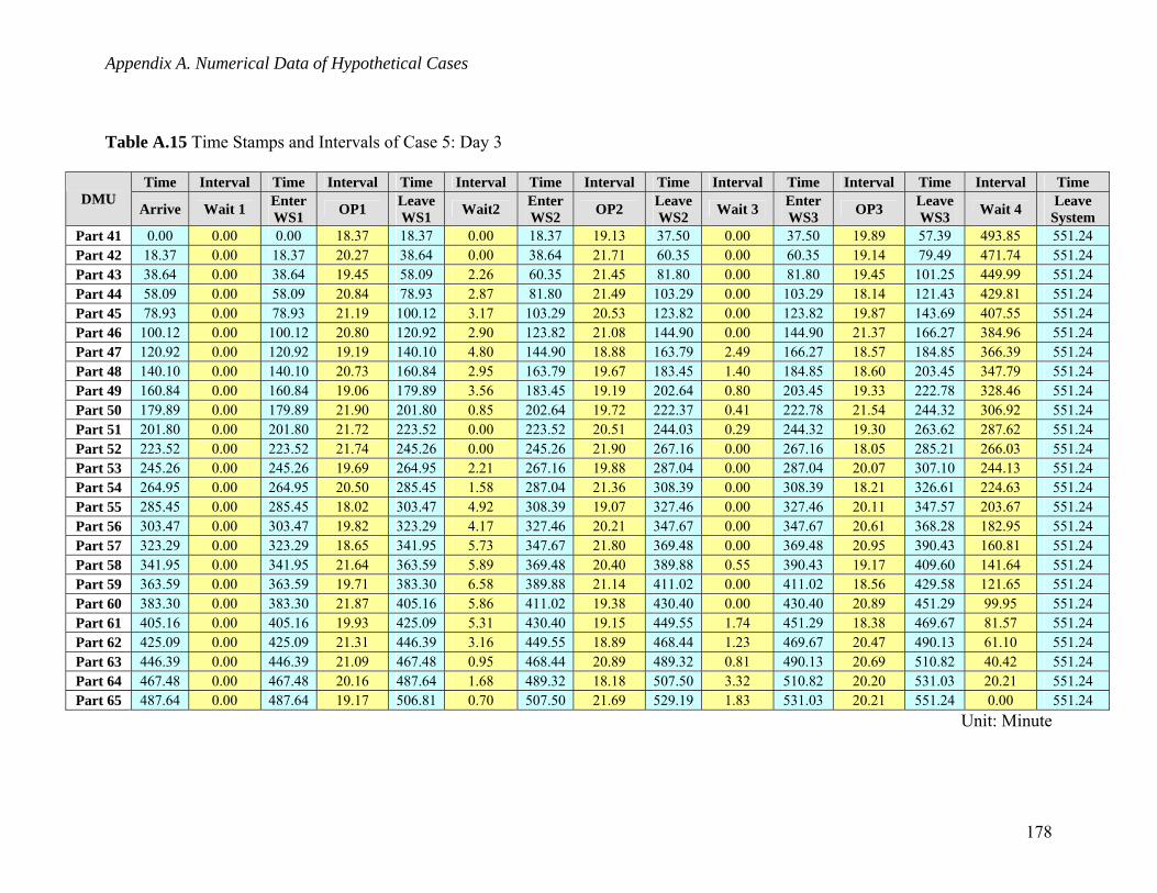
Appendix A. Numerical Data of Hypothetical Cases
Table A.15 Time Stamps and Intervals of Case 5: Day 3
Time Interval Time Interval Time Interval Time Interval Time Interval Time Interval Time Interval Time DMU
Arrive Wait 1 Enter WS1 OP1 Leave
WS1 Wait2 Enter WS2 OP2 Leave
WS2 Wait 3 Enter WS3 OP3 Leave
WS3 Wait 4 Leave System
Part 41 0.00 0.00 0.00 18.37 18.37 0.00 18.37 19.13 37.50 0.00 37.50 19.89 57.39 493.85 551.24 Part 42 18.37 0.00 18.37 20.27 38.64 0.00 38.64 21.71 60.35 0.00 60.35 19.14 79.49 471.74 551.24 Part 43 38.64 0.00 38.64 19.45 58.09 2.26 60.35 21.45 81.80 0.00 81.80 19.45 101.25 449.99 551.24 Part 44 58.09 0.00 58.09 20.84 78.93 2.87 81.80 21.49 103.29 0.00 103.29 18.14 121.43 429.81 551.24 Part 45 78.93 0.00 78.93 21.19 100.12 3.17 103.29 20.53 123.82 0.00 123.82 19.87 143.69 407.55 551.24 Part 46 100.12 0.00 100.12 20.80 120.92 2.90 123.82 21.08 144.90 0.00 144.90 21.37 166.27 384.96 551.24 Part 47 120.92 0.00 120.92 19.19 140.10 4.80 144.90 18.88 163.79 2.49 166.27 18.57 184.85 366.39 551.24 Part 48 140.10 0.00 140.10 20.73 160.84 2.95 163.79 19.67 183.45 1.40 184.85 18.60 203.45 347.79 551.24 Part 49 160.84 0.00 160.84 19.06 179.89 3.56 183.45 19.19 202.64 0.80 203.45 19.33 222.78 328.46 551.24 Part 50 179.89 0.00 179.89 21.90 201.80 0.85 202.64 19.72 222.37 0.41 222.78 21.54 244.32 306.92 551.24 Part 51 201.80 0.00 201.80 21.72 223.52 0.00 223.52 20.51 244.03 0.29 244.32 19.30 263.62 287.62 551.24 Part 52 223.52 0.00 223.52 21.74 245.26 0.00 245.26 21.90 267.16 0.00 267.16 18.05 285.21 266.03 551.24 Part 53 245.26 0.00 245.26 19.69 264.95 2.21 267.16 19.88 287.04 0.00 287.04 20.07 307.10 244.13 551.24 Part 54 264.95 0.00 264.95 20.50 285.45 1.58 287.04 21.36 308.39 0.00 308.39 18.21 326.61 224.63 551.24 Part 55 285.45 0.00 285.45 18.02 303.47 4.92 308.39 19.07 327.46 0.00 327.46 20.11 347.57 203.67 551.24 Part 56 303.47 0.00 303.47 19.82 323.29 4.17 327.46 20.21 347.67 0.00 347.67 20.61 368.28 182.95 551.24 Part 57 323.29 0.00 323.29 18.65 341.95 5.73 347.67 21.80 369.48 0.00 369.48 20.95 390.43 160.81 551.24 Part 58 341.95 0.00 341.95 21.64 363.59 5.89 369.48 20.40 389.88 0.55 390.43 19.17 409.60 141.64 551.24 Part 59 363.59 0.00 363.59 19.71 383.30 6.58 389.88 21.14 411.02 0.00 411.02 18.56 429.58 121.65 551.24 Part 60 383.30 0.00 383.30 21.87 405.16 5.86 411.02 19.38 430.40 0.00 430.40 20.89 451.29 99.95 551.24 Part 61 405.16 0.00 405.16 19.93 425.09 5.31 430.40 19.15 449.55 1.74 451.29 18.38 469.67 81.57 551.24 Part 62 425.09 0.00 425.09 21.31 446.39 3.16 449.55 18.89 468.44 1.23 469.67 20.47 490.13 61.10 551.24 Part 63 446.39 0.00 446.39 21.09 467.48 0.95 468.44 20.89 489.32 0.81 490.13 20.69 510.82 40.42 551.24 Part 64 467.48 0.00 467.48 20.16 487.64 1.68 489.32 18.18 507.50 3.32 510.82 20.20 531.03 20.21 551.24 Part 65 487.64 0.00 487.64 19.17 506.81 0.70 507.50 21.69 529.19 1.83 531.03 20.21 551.24 0.00 551.24
Unit: Minute
178
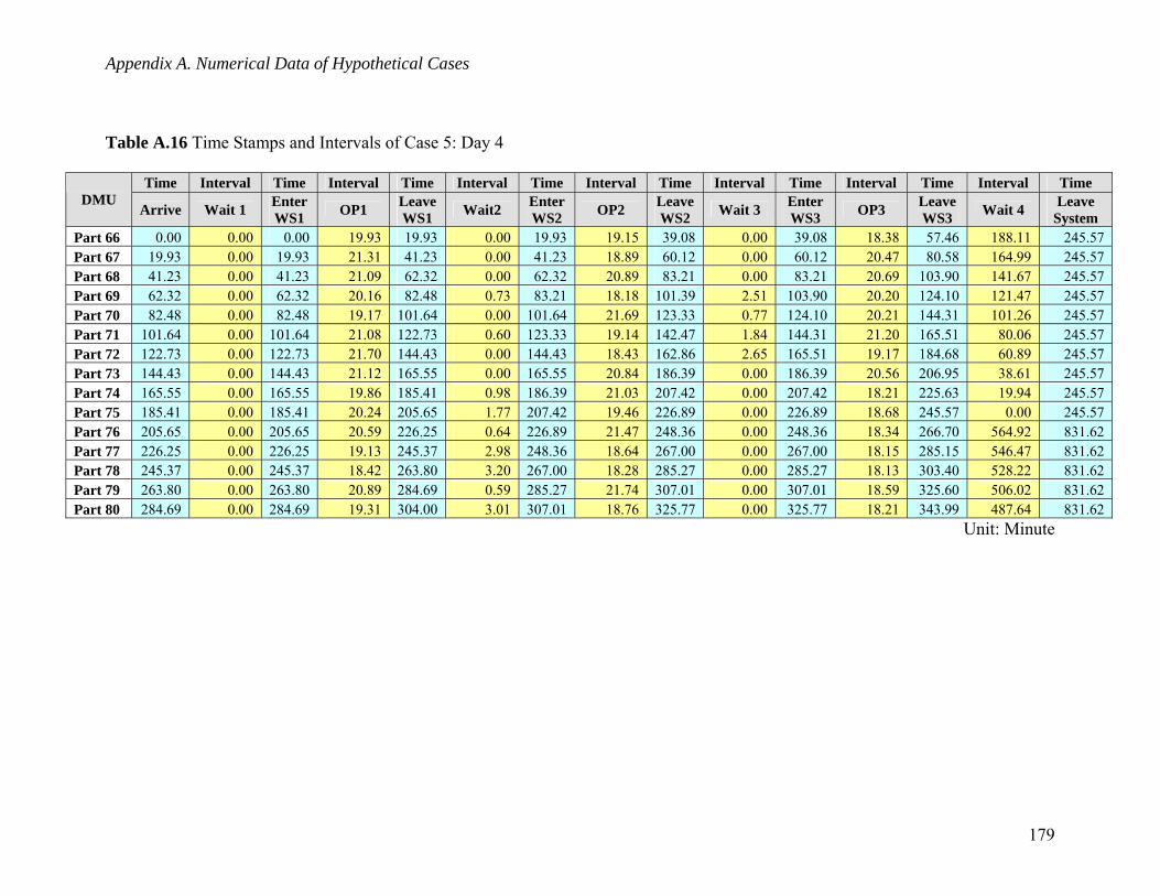
Appendix A. Numerical Data of Hypothetical Cases
Table A.16 Time Stamps and Intervals of Case 5: Day 4
Time Interval Time Interval Time Interval Time Interval Time Interval Time Interval Time Interval Time DMU
Arrive Wait 1 Enter WS1 OP1 Leave
WS1 Wait2 Enter WS2 OP2 Leave
WS2 Wait 3 Enter WS3 OP3 Leave
WS3 Wait 4 Leave System
Part 66 0.00 0.00 0.00 19.93 19.93 0.00 19.93 19.15 39.08 0.00 39.08 18.38 57.46 188.11 245.57 Part 67 19.93 0.00 19.93 21.31 41.23 0.00 41.23 18.89 60.12 0.00 60.12 20.47 80.58 164.99 245.57 Part 68 41.23 0.00 41.23 21.09 62.32 0.00 62.32 20.89 83.21 0.00 83.21 20.69 103.90 141.67 245.57 Part 69 62.32 0.00 62.32 20.16 82.48 0.73 83.21 18.18 101.39 2.51 103.90 20.20 124.10 121.47 245.57 Part 70 82.48 0.00 82.48 19.17 101.64 0.00 101.64 21.69 123.33 0.77 124.10 20.21 144.31 101.26 245.57 Part 71 101.64 0.00 101.64 21.08 122.73 0.60 123.33 19.14 142.47 1.84 144.31 21.20 165.51 80.06 245.57 Part 72 122.73 0.00 122.73 21.70 144.43 0.00 144.43 18.43 162.86 2.65 165.51 19.17 184.68 60.89 245.57 Part 73 144.43 0.00 144.43 21.12 165.55 0.00 165.55 20.84 186.39 0.00 186.39 20.56 206.95 38.61 245.57 Part 74 165.55 0.00 165.55 19.86 185.41 0.98 186.39 21.03 207.42 0.00 207.42 18.21 225.63 19.94 245.57 Part 75 185.41 0.00 185.41 20.24 205.65 1.77 207.42 19.46 226.89 0.00 226.89 18.68 245.57 0.00 245.57 Part 76 205.65 0.00 205.65 20.59 226.25 0.64 226.89 21.47 248.36 0.00 248.36 18.34 266.70 564.92 831.62 Part 77 226.25 0.00 226.25 19.13 245.37 2.98 248.36 18.64 267.00 0.00 267.00 18.15 285.15 546.47 831.62 Part 78 245.37 0.00 245.37 18.42 263.80 3.20 267.00 18.28 285.27 0.00 285.27 18.13 303.40 528.22 831.62 Part 79 263.80 0.00 263.80 20.89 284.69 0.59 285.27 21.74 307.01 0.00 307.01 18.59 325.60 506.02 831.62 Part 80 284.69 0.00 284.69 19.31 304.00 3.01 307.01 18.76 325.77 0.00 325.77 18.21 343.99 487.64 831.62
Unit: Minute
179
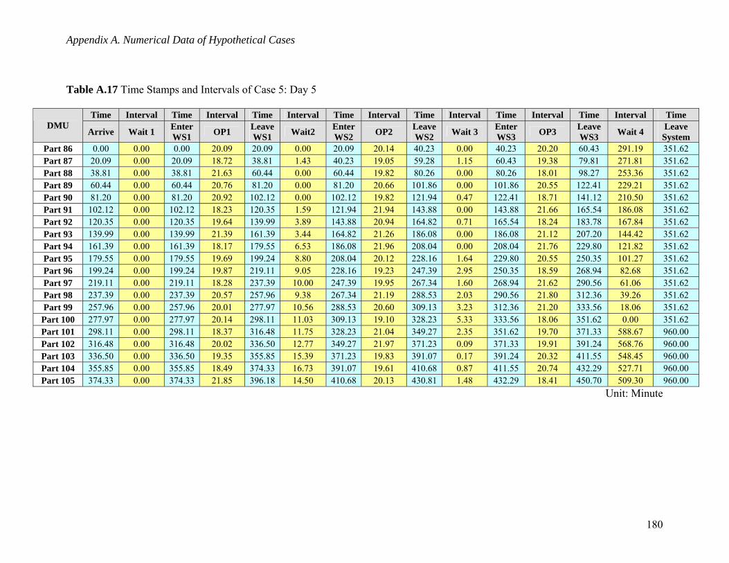
Appendix A. Numerical Data of Hypothetical Cases
Table A.17 Time Stamps and Intervals of Case 5: Day 5
Time Interval Time Interval Time Interval Time Interval Time Interval Time Interval Time Interval Time DMU
Arrive Wait 1 Enter WS1 OP1 Leave
WS1 Wait2 Enter WS2 OP2 Leave
WS2 Wait 3 Enter WS3 OP3 Leave
WS3 Wait 4 Leave System
Part 86 0.00 0.00 0.00 20.09 20.09 0.00 20.09 20.14 40.23 0.00 40.23 20.20 60.43 291.19 351.62 Part 87 20.09 0.00 20.09 18.72 38.81 1.43 40.23 19.05 59.28 1.15 60.43 19.38 79.81 271.81 351.62 Part 88 38.81 0.00 38.81 21.63 60.44 0.00 60.44 19.82 80.26 0.00 80.26 18.01 98.27 253.36 351.62 Part 89 60.44 0.00 60.44 20.76 81.20 0.00 81.20 20.66 101.86 0.00 101.86 20.55 122.41 229.21 351.62 Part 90 81.20 0.00 81.20 20.92 102.12 0.00 102.12 19.82 121.94 0.47 122.41 18.71 141.12 210.50 351.62 Part 91 102.12 0.00 102.12 18.23 120.35 1.59 121.94 21.94 143.88 0.00 143.88 21.66 165.54 186.08 351.62 Part 92 120.35 0.00 120.35 19.64 139.99 3.89 143.88 20.94 164.82 0.71 165.54 18.24 183.78 167.84 351.62 Part 93 139.99 0.00 139.99 21.39 161.39 3.44 164.82 21.26 186.08 0.00 186.08 21.12 207.20 144.42 351.62 Part 94 161.39 0.00 161.39 18.17 179.55 6.53 186.08 21.96 208.04 0.00 208.04 21.76 229.80 121.82 351.62 Part 95 179.55 0.00 179.55 19.69 199.24 8.80 208.04 20.12 228.16 1.64 229.80 20.55 250.35 101.27 351.62 Part 96 199.24 0.00 199.24 19.87 219.11 9.05 228.16 19.23 247.39 2.95 250.35 18.59 268.94 82.68 351.62 Part 97 219.11 0.00 219.11 18.28 237.39 10.00 247.39 19.95 267.34 1.60 268.94 21.62 290.56 61.06 351.62 Part 98 237.39 0.00 237.39 20.57 257.96 9.38 267.34 21.19 288.53 2.03 290.56 21.80 312.36 39.26 351.62 Part 99 257.96 0.00 257.96 20.01 277.97 10.56 288.53 20.60 309.13 3.23 312.36 21.20 333.56 18.06 351.62
Part 100 277.97 0.00 277.97 20.14 298.11 11.03 309.13 19.10 328.23 5.33 333.56 18.06 351.62 0.00 351.62 Part 101 298.11 0.00 298.11 18.37 316.48 11.75 328.23 21.04 349.27 2.35 351.62 19.70 371.33 588.67 960.00 Part 102 316.48 0.00 316.48 20.02 336.50 12.77 349.27 21.97 371.23 0.09 371.33 19.91 391.24 568.76 960.00 Part 103 336.50 0.00 336.50 19.35 355.85 15.39 371.23 19.83 391.07 0.17 391.24 20.32 411.55 548.45 960.00 Part 104 355.85 0.00 355.85 18.49 374.33 16.73 391.07 19.61 410.68 0.87 411.55 20.74 432.29 527.71 960.00 Part 105 374.33 0.00 374.33 21.85 396.18 14.50 410.68 20.13 430.81 1.48 432.29 18.41 450.70 509.30 960.00
Unit: Minute
180
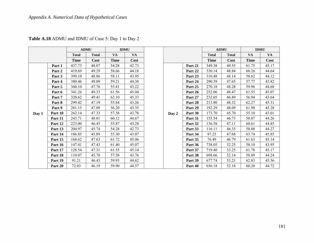
Appendix A. Numerical Data of Hypothetical Cases
Table A.18 ADMU and IDMU of Case 5: Day 1 to Day 2
ADMU IDMU ADMU IDMU Total Total VA VA Total Total VA VA
Time Cost Time Cost
Time Cost Time Cost Part 1 437.73 48.07 54.28 42.73 Part 21 349.38 49.55 61.75 45.17 Part 2 419.69 49.29 58.66 44.18 Part 22 330.14 48.84 60.26 44.64 Part 3 399.10 48.86 58.11 43.95 Part 23 310.48 48.14 58.62 44.12 Part 4 380.46 49.09 59.21 44.38 Part 24 290.39 47.65 57.77 43.82 Part 5 360.10 47.76 55.81 43.22 Part 25 270.18 48.28 59.96 44.68 Part 6 341.26 49.33 61.56 45.04 Part 26 252.06 48.47 61.55 45.07 Part 7 320.62 49.41 62.10 45.33 Part 27 232.05 46.89 56.94 43.64 Part 8 299.42 47.19 55.84 43.26 Part 28 213.80 48.32 62.27 45.31 Part 9 281.15 47.09 56.20 43.35 Part 29 192.29 48.09 61.98 45.28 Part 10 262.14 47.33 57.38 43.78 Part 30 173.70 45.70 55.10 43.01 Part 11 243.71 48.01 60.12 44.67 Part 31 155.54 46.73 58.87 44.26 Part 12 223.00 46.45 55.87 43.28 Part 32 136.58 47.11 60.61 44.85 Part 13 204.97 45.74 54.28 42.73 Part 33 116.11 46.35 58.88 44.27 Part 14 186.85 45.89 55.30 43.07 Part 34 97.25 47.68 63.74 45.85 Part 15 168.62 47.63 61.72 45.06 Part 35 76.49 46.79 61.63 45.14 Part 16 147.41 47.43 61.40 45.07 Part 36 738.05 52.25 58.10 43.95 Part 17 128.54 47.31 61.55 45.14 Part 37 719.40 53.25 61.78 45.17 Part 18 110.07 45.78 57.58 43.76 Part 38 698.66 52.14 58.89 44.24 Part 19 91.21 46.43 59.93 44.62 Part 39 677.74 53.21 62.83 45.56
Day 1
Part 20 72.03 46.19 59.90 44.57
Day 2
Part 40 656.18 52.18 60.20 44.72
181
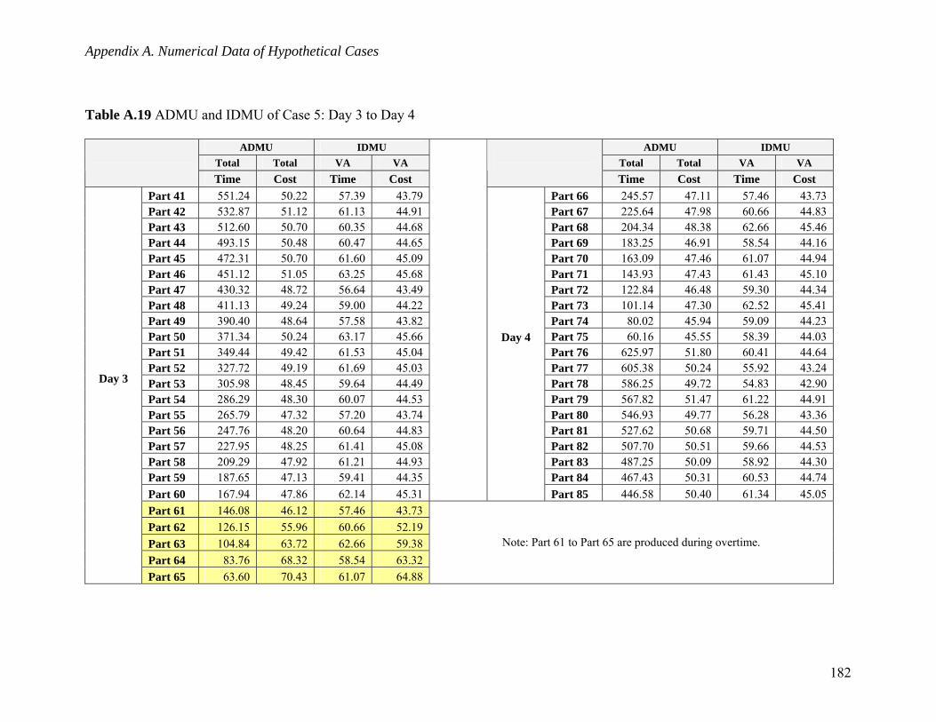
Appendix A. Numerical Data of Hypothetical Cases
Table A.19 ADMU and IDMU of Case 5: Day 3 to Day 4
ADMU IDMU ADMU IDMU Total Total VA VA Total Total VA VA
Time Cost Time Cost
Time Cost Time Cost Part 41 551.24 50.22 57.39 43.79 Part 66 245.57 47.11 57.46 43.73 Part 42 532.87 51.12 61.13 44.91 Part 67 225.64 47.98 60.66 44.83 Part 43 512.60 50.70 60.35 44.68 Part 68 204.34 48.38 62.66 45.46 Part 44 493.15 50.48 60.47 44.65 Part 69 183.25 46.91 58.54 44.16 Part 45 472.31 50.70 61.60 45.09 Part 70 163.09 47.46 61.07 44.94 Part 46 451.12 51.05 63.25 45.68 Part 71 143.93 47.43 61.43 45.10 Part 47 430.32 48.72 56.64 43.49 Part 72 122.84 46.48 59.30 44.34 Part 48 411.13 49.24 59.00 44.22 Part 73 101.14 47.30 62.52 45.41 Part 49 390.40 48.64 57.58 43.82 Part 74 80.02 45.94 59.09 44.23 Part 50 371.34 50.24 63.17 45.66 Part 75 60.16 45.55 58.39 44.03 Part 51 349.44 49.42 61.53 45.04 Part 76 625.97 51.80 60.41 44.64 Part 52 327.72 49.19 61.69 45.03 Part 77 605.38 50.24 55.92 43.24 Part 53 305.98 48.45 59.64 44.49 Part 78 586.25 49.72 54.83 42.90 Part 54 286.29 48.30 60.07 44.53 Part 79 567.82 51.47 61.22 44.91 Part 55 265.79 47.32 57.20 43.74 Part 80 546.93 49.77 56.28 43.36 Part 56 247.76 48.20 60.64 44.83 Part 81 527.62 50.68 59.71 44.50 Part 57 227.95 48.25 61.41 45.08 Part 82 507.70 50.51 59.66 44.53 Part 58 209.29 47.92 61.21 44.93 Part 83 487.25 50.09 58.92 44.30 Part 59 187.65 47.13 59.41 44.35 Part 84 467.43 50.31 60.53 44.74 Part 60 167.94 47.86 62.14 45.31
Day 4
Part 85 446.58 50.40 61.34 45.05 Part 61 146.08 46.12 57.46 43.73 Part 62 126.15 55.96 60.66 52.19 Part 63 104.84 63.72 62.66 59.38 Part 64 83.76 68.32 58.54 63.32
Day 3
Part 65 63.60 70.43 61.07 64.88
Note: Part 61 to Part 65 are produced during overtime.
182
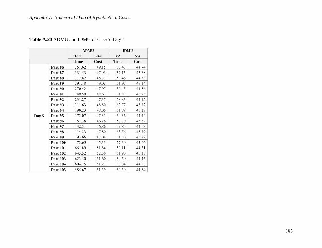
Appendix A. Numerical Data of Hypothetical Cases
Table A.20 ADMU and IDMU of Case 5: Day 5
ADMU IDMU Total Total VA VA
Time Cost Time Cost
Part 86 351.62 49.15 60.43 44.74 Part 87 331.53 47.93 57.15 43.68 Part 88 312.82 48.37 59.46 44.33 Part 89 291.18 49.03 61.97 45.24 Part 90 270.42 47.97 59.45 44.36 Part 91 249.50 48.63 61.83 45.25 Part 92 231.27 47.37 58.83 44.15 Part 93 211.63 48.80 63.77 45.82 Part 94 190.23 48.06 61.89 45.27 Part 95 172.07 47.35 60.36 44.74 Part 96 152.38 46.26 57.70 43.82 Part 97 132.51 46.86 59.85 44.63 Part 98 114.23 47.80 63.56 45.79 Part 99 93.66 47.04 61.80 45.22 Part 100 73.65 45.33 57.30 43.66 Part 101 661.89 51.84 59.11 44.31 Part 102 643.52 52.50 61.90 45.18 Part 103 623.50 51.60 59.50 44.46 Part 104 604.15 51.23 58.84 44.28
Day 5
Part 105 585.67 51.39 60.39 44.64
183

Appendix B. VBA Controller Program for Excel-based DEA-Leanness Solver
Appendix B. VBA Controller Program for Excel-based DEA-Leanness Solver Sub SBM_LP() ' ' DEA-SBM-LP Model for Leanness Measure of 60 DMUs ' Modified from Course Material ' ISE 5144 Performance and Productivity Measurement and Evaluation ' Dr. K. Triantis (Virginia Tech) ' ' Edited by Hung-da Wan ' Application.ScreenUpdating = False Dim n As Integer Sheets("SBM_results").Select Sheets("SBM_results").Range("B3").Select For n = 1 To 60 Sheets("SBM_model").Select Sheets("SBM_model").Range("A67").Value = n SolverOk SetCell:="$G$69", MaxMinVal:=2, ValueOf:=0, ByChange:= _ "$D$69,$G$70,$J$73:$L$73,$F$3:$F$62" SolverSolve (True) Sheets("SBM_model").Select Range("D69").Copy Sheets("SBM_results").Select ActiveCell.PasteSpecial Paste:=xlValue, Operation:=xlNone, SkipBlanks:= _ False, Transpose:=False ActiveCell.Offset(0, 1).Select Range("J76:L76").Copy Sheets("SBM_results").Select ActiveCell.PasteSpecial Paste:=xlValues, Operation:=xlNone, SkipBlanks:= _ False, Transpose:=False ActiveCell.Offset(0, 3).Select Range("G3:G62").Copy Sheets("SBM_results").Select ActiveCell.PasteSpecial Paste:=xlValues, Operation:=xlNone, SkipBlanks:= _ False, Transpose:=True
184
Appendix B. VBA Controller Program for Excel-based DEA-Leanness Solver
ActiveCell.Offset(1, -4).Select Next n End Sub *Note: The cells of the spreadsheet are constructed to represent the data, objective function, and constraints of the SBM model as introduced in Section 6.2.1.
185

Vita
Vita
Hung-da Wan was born in Taipei, Taiwan, in 1971. He received his B.S. degree
in Mechanical Engineering from National Taiwan University (NTU) in 1994. With his
strong interests in mechanical design, he won two titles in technology contests and
received one patent of new design during his undergraduate years. He continued his
studies in NTU and received his M.S. degree in Industrial Engineering in 1996. His thesis,
“Computer Integrated Rapid Prototyping and Reverse Engineering” supervised by Dr.
Ming-tzong Wang, was a pioneering work among researchers in Taiwan in the mid
1990’s. After serving two years in the army, he joined Mady Enterprise, one of the major
trading companies in bicycle and sporting goods in Taiwan. He started as a project leader
of product development and then became the manager of second division conducting
product developments and marketing of bicycles, exercisers, and automobile parts until
June 2002. His team brought out several new models of electric light vehicles and
received the “Best Design Award” of Year 2001 from the China External Trade
Development Council in Taiwan. During the four years of tenure in industry, he visited
various types of manufacturing facilities in several countries, which inspired him to
pursue further knowledge in the field of industrial engineering.
He entered the Ph.D. program in the Grado Department of Industrial and Systems
Engineering at Virginia Tech, Manufacturing Systems Engineering Option, in August
2002. At the same time, he joined the Center for High Performance Manufacturing
(CHPM) as a graduate research assistant under the direction of Dr. F. Frank Chen. Wan’s
major research interests include Lean Manufacturing, Web-based Manufacturing Systems,
Performance Measurement, and Lean Supply Chain. One of his works, “Decision
Support and Analysis Tool for Lean Manufacturing Assessment and Implementation,”
delivered a software program copyrighted in 2005. He also contributed to the research
project “Enhanced Lean Manufacturing and Six-sigma Integration” and led the major
R&D activities in the project “Flexible Web-based Kanban System.” He is a recipient of
2003-2004 Dover Endowed ISE Fellowship Award.
186