Measuring Water Conductivity with Polarized Electrodes

69

RESEARCH ARTICLE

Replication Attempt: Measuring Water

Conductivity with Polarized Electrodes

SERGE KERNBACH

Institute of Parallel and Distributed Systems, University of Stuttgart, Universitätstrasse 38, Stuttgart 70569, [email protected]

Submitted 3/12/2012, Accepted 11/23/2012, Prepublished 1/15/2013

Abstract—We attempted to reproduce the results of experiments related to measuring the conductivity of water with deeply polarized electrodes. As proposed in the original works, the polarized electrodes are sensitive to a high-penetrating emission generated by objects of diff erent origin. We demonstrate the experiment setup used and the results obtained in replica-tion and control experiments. Based on the trials carried out, we judge the results of this replication to be positive.

Introduction

This study is based on previous research related to underwater communication by means of electric fi elds. This approach is inspired by weakly electric fi sh (von der Emde, Schwarz, Gomez, Budelli, & Grant 1998, Sim & Kim, 2011) that use different features of electric fi elds for navigation, sensing, and the coordination of collective activities. The equipment for the generation and sensing of electric fi elds is installed on small mobile underwater devices (Kernbach, Dipper, & Sutantyo 2011, Dipper, Gebhardt, Kernbach, & von der Emde 2011). The fi elds produced by different devices interact with each other and provide an account of the global properties of the underwater environment (Schmickl, Thenius, Moslinger, Timmis, Tyrell, et al., 2011). In several experiments, the modulation frequency of the electric fi eld is very low (in the range of 0.01 to 0.001 Hz), which creates deeply polarized electrodes.

In carrying out these experiments on communication via electric fi elds, we noted two interesting effects. First, the results obtained are highly reproducible for relative values within one experiment. However, in the cases of deeply polarized electrodes, the results vary among experiments. The main factors identifi ed, which infl uenced many of the results, included sensitivity to mechanical vibrations, the emissions of blue-light LEDs (used for navigation purposes), and the duration of the experiment.

Journal of Scientifi c Exploration, Vol. 27, No. 1, pp. 69–105, 2013 0892-3310/13

70 Serge Kernbach

Several works report sensitivity in polarized electrodes to laser and LED light, and ultrasonic waves (Bobrov 2006, 1998). These works are denoted as lying within the fi eld of research related to “non-electromagnetic” (non-EM) fi elds. Despite controversial discussions, we also make use of this notion, because the original papers introduced it to explain the effects discovered in the electric double layer (EDL) (Muzalewskay & Bobrov 1988). The diffusion Gouy–Chapman layer in EDL is sensitive to, among other things, a spatial polarization of water dipoles, e.g., Lyklema (2005) and Belaya, Feigel’man, and Levadnyii (1987). Eliminating such factors as variation of temperature, EM fi elds, or vibrations, the authors Muzalewskay and Bobrov (1988) demonstrated that some active or passive objects can change the dielectric properties of EDL. These changes are detectable by measuring the current fl owing through the water–electrode system. As noted in existing research, for instance in Bobrov (2006), experiments are carried out not only with non-biological but also with biological objects such as seeds or bacteria (Bobrov 1992). Thus, the deeply polarized electrodes in water might represent a detector, which is sensitive to possible non-EM fi elds.

In particular, we are interested in the following experiment: polarized electrodes in a small container with water, representing a detector. Several such detectors were placed inside a metal box, protected from EM fi elds and temperature changes. Electronic equipment measured the conductivity of water in each of the detectors and recorded its dynamics. An LED generator was prepared, consisting of 128 yellow-light super-bright LEDs. Another container of water was irradiated by this LED generator (Bobrov 2002). As stated in Bobrov (2009, 2006), the detectors demonstrated different dynamics in the presence of irradiated water, normal water, and control experiments. In other words, the impact of non-EM fi elds from the LED generator is measurable not only directly but also indirectly through irradiated water. Since mechanical, acoustic, optical, capacitive, temperature, and EM infl uences were excluded from these experiments, the polarization of water dipoles by the LED generator created a number of deep scientifi c questions related to the nature of this interaction.

We decided to replicate this experiment in the context of our research. Primarily, the goal was not only to confi rm or refute the results of the experiment above, but also to estimate the value of a possible non-EM component and its use in the context of underwater communication. We changed the conditions of the experiments and compared the dynamics of the water conductivity (current fl owing though the water at a constant voltage) in the presence of (a) an active LED generator, (b) water irradiated by the LED generator, (c) normal water, and (d) control experiments. Comparing the dynamics of (a) and (b) to (d) could provide an account of

Measuring Water Conductivity with Polarized Electrodes 71

a possible non-EM fi eld and comparing (b) to (c) an account of the degree of spatial polarization of the water dipoles. Since conductivity is measured by a small current, we paid close attention to technical issues of accurate measurement and experimental reproducibility.

This article is structured as follows: The Methodology section describes the methodology and measurement approach used. The experiment setup is described in Appendix A. We performed three experiment series: series “A”—calibration and preliminary experiments, as described in the section Characterization of Sensors: Impact of Temperature, Vibration, and EM fi elds; series “C”—measuring the conductivity of water under the infl uence of the LED generator and irradiated water, as described in the section Experiment Series C. Additionally, in series “B” we measured the conductivity of water related to non-EM fi elds of biological origin (as described for example in Bobrov (2006)); however, these experiments are excluded from this work. Finally, in the sections Discussion of Results and Conclusion we generalize from the experiments carried out and conclude this paper.

Methodology

The electric double layer (EDL) appears on the surface of an object placed into a liquid. Electrokinetic phenomena are described by the Gouy–Chapman–Stern model (Lyklema 2005). Corresponding to this model, EDL can be represented by two layers: the internal Helmholtz (absorption) layer and the outer Gouy–Chapman (diffuse) layer (Kornyshev 2007). As mentioned in Bobrov (2006), the diffuse layer is of interest. In a number of works, e.g., Stenschke (1985), David, Gruen, and Marcelja (1983), and Belaya, Feigel’man, and Levadnyii (1987), dielectric behavior and properties of the Gouy–Chapman layer are investigated. In particular, the dielectric response of this layer depends on among other factors the temperature, ionic concentration, and spatial polarization of water dipoles. As proposed in the original works, e.g., Bobrov (2009), and confi rmed by a large number of different experiments, some non-biological as well as biological objects are capable of infl uencing the spatial polarization of dipoles and thus change dielectric properties of the Gouy–Chapman layer. Despite the fact that the principles of such an infl uence are not defi nitively identifi ed at the moment, the produced effects appeared in changing an electric current fl owing through the water–electrode system and thus can be experimentally measured. The main methodology of those experiments consisted of removing such factors as variation of temperature and EM fi elds, acoustic impacts, and vibrations from infl uence on the results. For statistical analysis the measurements are done by several sensors in parallel

72 Serge Kernbach

and repeated to achieve statistical signifi cance. This methodology is also adapted for our experiments.

We developed our own sensors by following the state of the art in conductometry. Conductometric analysis is a well-known approach that measures the conductivity of water. There are several different methods, using two or four electrodes, see Kirkham and Taylor (1949) or more recently Bristow, Kluitenberg, Goding, and Fitzgerald (2001), as well as inductive approaches. Generally, the results of measurements are infl uenced by (Orion Conductivity Theory no date):

• polarization of electrodes, that is appearance of EDL (Lyklema 2005);• temperature;• fringing effect of the electric fi eld (Parker 2002);• technical reasons, such as noise from the voltage generator, resistance of cables and connectors;• contamination of electrode surfaces.

In the vast literature, the process leading to an appearance of EDL is denoted as polarization of electrodes (Lyklema 2005). For conductometric purposes, the electrode polarization leads to a measurement error and therefore is undesirable. To minimize this error, the conductometry with two and four electrodes is performed with an AC voltage of up to 10 kHz frequency, see for example Spillner (1957). When using EDL as a sensor, the polarization of electrodes is required and takes about 6–8 hrs. To underline the difference from a normal conductometric analysis, such electrodes are denoted as deeply polarized electrodes.

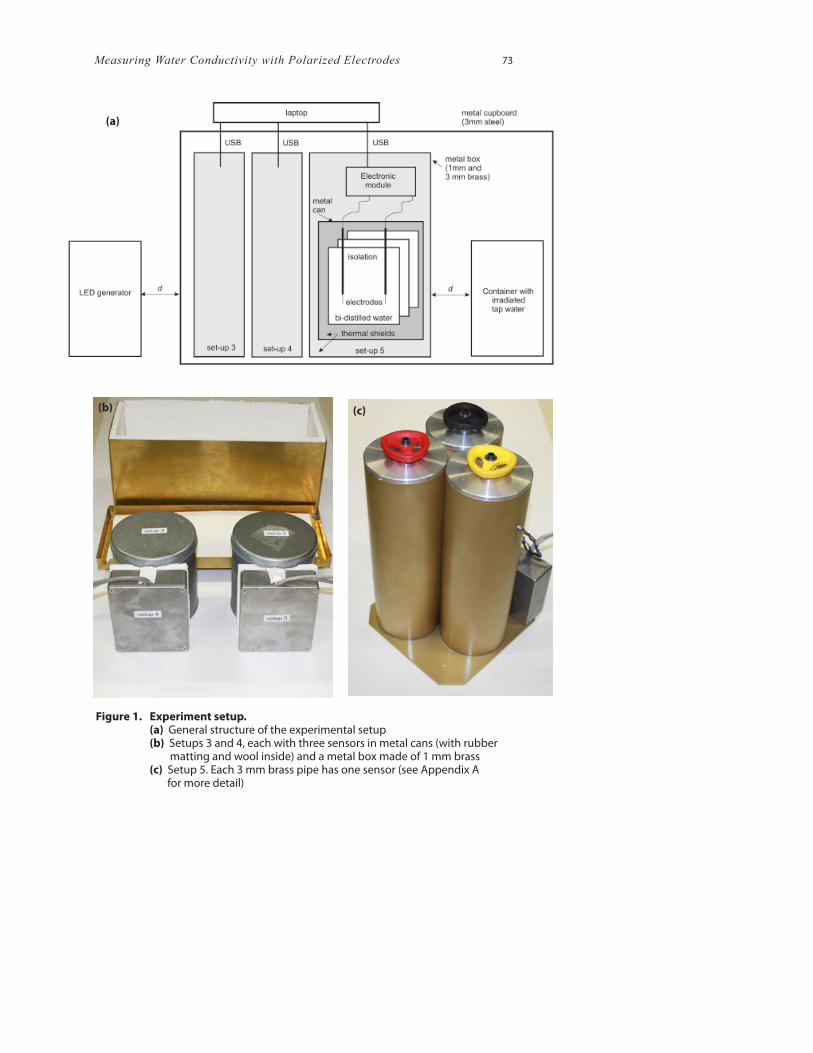
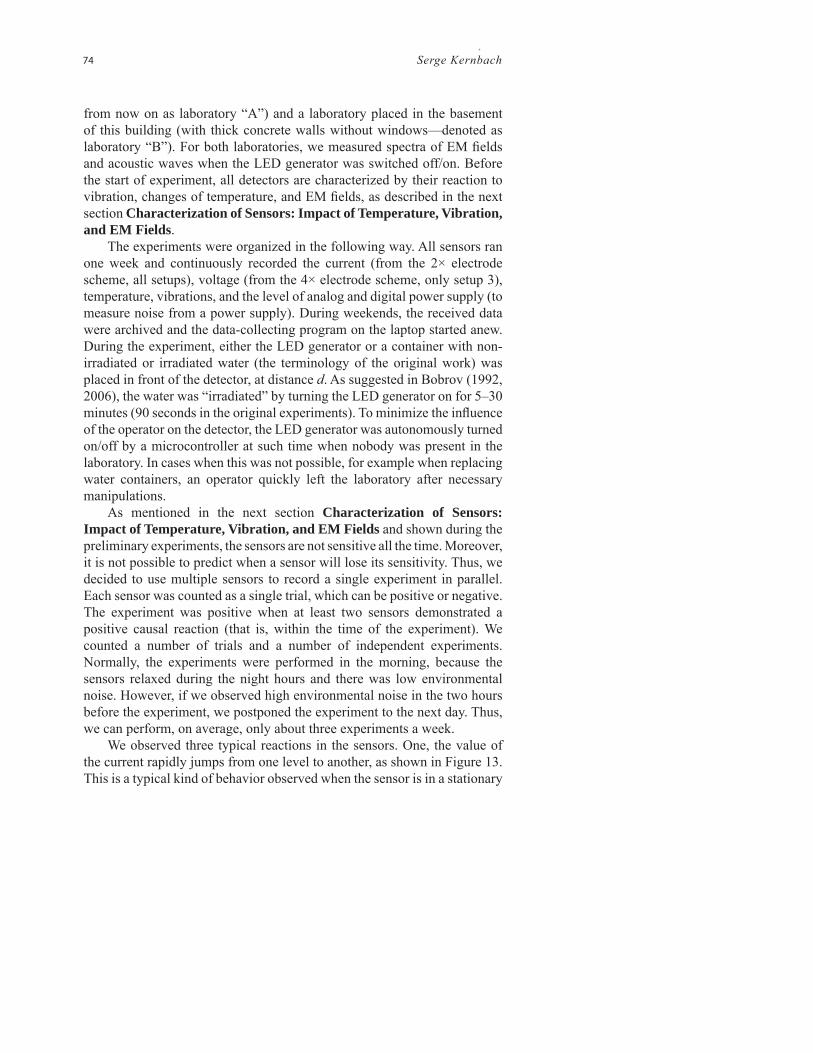
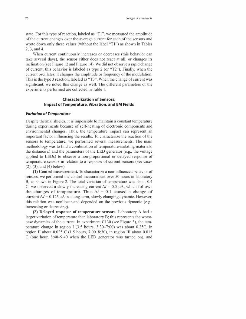
For our experiments, we prepared and used fi ve setups, as described in Appendix A (see four setups in Figure 19). The difference between them lies in the material, placement, and number of electrodes. In the following, we denote each set of electrodes in containers with water as sensors. Three identical sensors are collected into one setup, controlled by one microcontroller. For experiments, we used setups 3, 4, and 5 with nine sensors in total. To counter the infl uence of EM fi elds and parasitic couplings, the water containers with electrodes were inserted into several grounded metal boxes lined with rubber matting and wool (see Figure 1). Finally, detectors and the container with irradiated water were placed into a closed metal cupboard (the LED generator was placed outside the cupboard). The purpose of such multiple EM and temperature shields is to minimize the impact of temperature variation and environmental EM fi elds.

All experiments were performed in two laboratories: the normal electronic laboratory on the second fl oor of a university building (denoted


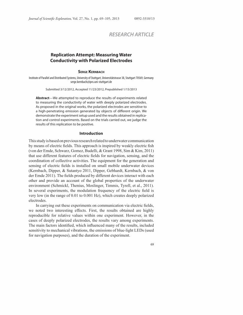
Figure 1. Experiment setup. (a) General structure of the experimental setup (b) Setups 3 and 4, each with three sensors in metal cans (with rubber matting and wool inside) and a metal box made of 1 mm brass (c) Setup 5. Each 3 mm brass pipe has one sensor (see Appendix A for more detail)

(a)

(b) (c)

74 Serge Kernbach

from now on as laboratory “A”) and a laboratory placed in the basement of this building (with thick concrete walls without windows—denoted as laboratory “B”). For both laboratories, we measured spectra of EM fi elds and acoustic waves when the LED generator was switched off/on. Before the start of experiment, all detectors are characterized by their reaction to vibration, changes of temperature, and EM fi elds, as described in the next section Characterization of Sensors: Impact of Temperature, Vibration, and EM Fields.

The experiments were organized in the following way. All sensors ran one week and continuously recorded the current (from the 2× electrode scheme, all setups), voltage (from the 4× electrode scheme, only setup 3), temperature, vibrations, and the level of analog and digital power supply (to measure noise from a power supply). During weekends, the received data were archived and the data-collecting program on the laptop started anew. During the experiment, either the LED generator or a container with non-irradiated or irradiated water (the terminology of the original work) was placed in front of the detector, at distance d. As suggested in Bobrov (1992, 2006), the water was “irradiated” by turning the LED generator on for 5–30 minutes (90 seconds in the original experiments). To minimize the infl uence of the operator on the detector, the LED generator was autonomously turned on/off by a microcontroller at such time when nobody was present in the laboratory. In cases when this was not possible, for example when replacing water containers, an operator quickly left the laboratory after necessary manipulations.

As mentioned in the next section Characterization of Sensors: Impact of Temperature, Vibration, and EM Fields and shown during the preliminary experiments, the sensors are not sensitive all the time. Moreover, it is not possible to predict when a sensor will lose its sensitivity. Thus, we decided to use multiple sensors to record a single experiment in parallel. Each sensor was counted as a single trial, which can be positive or negative. The experiment was positive when at least two sensors demonstrated a positive causal reaction (that is, within the time of the experiment). We counted a number of trials and a number of independent experiments. Normally, the experiments were performed in the morning, because the sensors relaxed during the night hours and there was low environmental noise. However, if we observed high environmental noise in the two hours before the experiment, we postponed the experiment to the next day. Thus, we can perform, on average, only about three experiments a week.

We observed three typical reactions in the sensors. One, the value of the current rapidly jumps from one level to another, as shown in Figure 13. This is a typical kind of behavior observed when the sensor is in a stationary


TABLE 1

Parameters of Experiment C

N Parameter Description

1 Type of electrodes Setup 3: 4-electrode scheme, chromium–stainless steel, 1 mm diameter (replaceable); Setup 4: 2-electrode scheme, fi rst electrode chromium–stainless steel, 1 mm diameter (replaceable); Setup 5: 2-electrode scheme, platinum, 1 mm diameter (non-replaceable)

2 Distance between electrodes 10 mm – 60 mm

3 Voltage level DC, 0.9 V – 4 V, changing of polarity is possible, noise level ±10 mV

4 Current level in DAC circuit 3 μA – 40 μA

5 EM (radio frequency and 50/60 Hz) and optical shield

All electrodes/electronics are placed inside several grounded metal boxes made of steel/brass. See Ott (1988) for more detail on EM production.

6 Temperature shield Foam rubber and wool in each metal box

7 Elimination of parasitic DC couplings Power via USB from a laptop, laptop in battery mode (in control experiments), LED generator powered by D-size batteries

8 Water used in sensors Purifi ed by osmosis (before Experiment C160) and bi-distilled (after Experiment C160), 50–150 ml in glass (setups 3 and 5) and stainless steel (setup 4) containers

9 Water used for irradiation Normal tap water, rested for 7–24 hours before the irradiation, 500 ml in glass container

10 Water used in control experiments Normal tap water, rested for 7–120 hours before the experiments, 500 ml in glass container

11 Type of sensor’s reaction Type 1, type 2, type 3

12 Exposure time of LED generator 20–40 minutes by 169 blue-light (470 nm), 11 cd LEDs

13 LED mode used in experiments Oscillations 1 and 2, rotation CCW and CW

14 Exposure time of irradiated water 30–80 minutes

15 Duration of irradiation of water 5–30 minutes

16 Distance between detector and LED generator / irradiated water

5–13, 30 cm

17 Time between irradiation of water and start of experiment

Immediately before, to 72 hours before

18 Number of sensors recording in parallel 3, 6, 9

76 Serge Kernbach

state. For this type of reaction, labeled as “T1”, we measured the amplitude of the current changes over the average current for each of the sensors and wrote down only these values (without the label “T1”) as shown in Tables 2, 3, and 4.

When current continuously increases or decreases (this behavior can take several days), the sensor either does not react at all, or changes its inclination (see Figure 12 and Figure 14). We did not observe a rapid change of current; this behavior is labeled as type 2 (or “T2”). Finally, when the current oscillates, it changes the amplitude or frequency of the modulation. This is the type 3 reaction, labeled as “T3”. When the change of current was signifi cant, we noted this change as well. The different parameters of the experiments performed are collected in Table 1.

Characterization of Sensors:

Impact of Temperature, Vibration, and EM Fields

Variation of Temperature

Despite thermal shields, it is impossible to maintain a constant temperature during experiments because of self-heating of electronic components and environmental changes. Thus, the temperature impact can represent an important factor infl uencing the results. To characterize the reaction of the sensors to temperature, we performed several measurements. The main methodology was to fi nd a combination of temperature-isolating materials, the distance d, and the parameters of the LED generator (e.g., the voltage applied to LEDs) to observe a non-proportional or delayed response of temperature sensors in relation to a response of current sensors (see cases (2), (3), and (4) below).

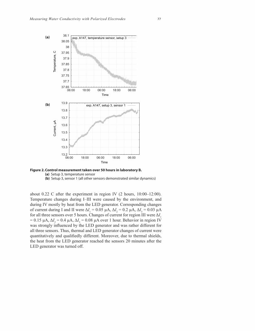
(1) Control measurement. To characterize a non-infl uenced behavior of sensors, we performed the control measurement over 50 hours in laboratory B, as shown in Figure 2. The total variation of temperature was about 0.4 C; we observed a slowly increasing current ΔI = 0.5 μA, which follows the changes of temperature. Thus Δt = 0.1 caused a change of current ΔI = 0.125 μA in a long-term, slowly changing dynamic. However, this relation was nonlinear and depended on the previous dynamic (e.g., increasing or decreasing).

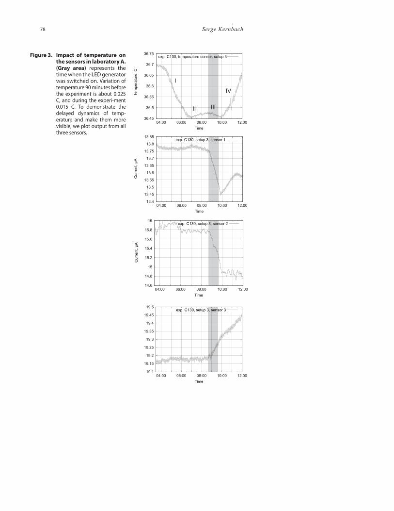
(2) Delayed response of temperature sensors. Laboratory A had a larger variation of temperature than laboratory B; this represents the worst-case dynamics of the current. In experiment C130 (see Figure 3), the tem-perature change in region I (3.5 hours, 3:30–7:00) was about 0.25C, in region II about 0.025 C (1.5 hours, 7:00–8:30), in region III about 0.015 C (one hour, 8:40–9:40 when the LED generator was turned on), and


about 0.22 C after the experiment in region IV (2 hours, 10:00–12:00). Temperature changes during I–III were caused by the environment, and during IV mostly by heat from the LED generator. Corresponding changes of current during I and II were ΔI1 = 0.05 μA, ΔI2 = 0.2 μA, ΔI3 = 0.03 μA for all three sensors over 5 hours. Changes of current for region III were ΔI1 = 0.15 μA, ΔI2 = 0.4 μA, ΔI3 = 0.08 μA over 1 hour. Behavior in region IV was strongly infl uenced by the LED generator and was rather different for all three sensors. Thus, thermal and LED generator changes of current were quantitatively and qualifi edly different. Moreover, due to thermal shields, the heat from the LED generator reached the sensors 20 minutes after the LED generator was turned off.

Figure 2. Control measurement taken over 50 hours in laboratory B. (a) Setup 3, temperature sensor (b) Setup 3, sensor 1 (all other sensors demonstrated similar dynamics)

37.65

37.7

37.75

37.8

37.85

37.9

37.95

38

38.05

38.1

06:00 18:00 06:00 18:00 06:00

Te

mp

era

ture

, C

Time

exp. A147, temperature sensor, setup 3

13.2

13.3

13.4

13.5

13.6

13.7

13.8

13.9

06:00 18:00 06:00 18:00 06:00

Cu

rre

nt,

μA

Time

exp. A147, setup 3, sensor 1

(a)

(b)

78 Serge Kernbach

Figure 3. Impact of temperature on the sensors in laboratory A.

(Gray area) represents the time when the LED generator was switched on. Variation of temperature 90 minutes before the experiment is about 0.025 C, and during the experi-ment 0.015 C. To demonstrate the delayed dynamics of temp-erature and make them more visible, we plot output from all three sensors.

IV

IIIII

I

36.45

36.5

36.55

36.6

36.65

36.7

36.75

04:00 06:00 08:00 10:00 12:00

Tem

pera

ture

, C

Time

exp. C130, temperature sensor, setup 3

13.4

13.45

13.5

13.55

13.6

13.65

13.7

13.75

13.8

13.85

04:00 06:00 08:00 10:00 12:00

Curr

ent, μ

A

Time

exp. C130, setup 3, sensor 1

14.6

14.8

15

15.2

15.4

15.6

15.8

16

04:00 06:00 08:00 10:00 12:00

Curr

ent, μ

A

Time


19.1

19.15

19.2

19.25

19.3

19.35

19.4

19.45

19.5

04:00 06:00 08:00 10:00 12:00

Time



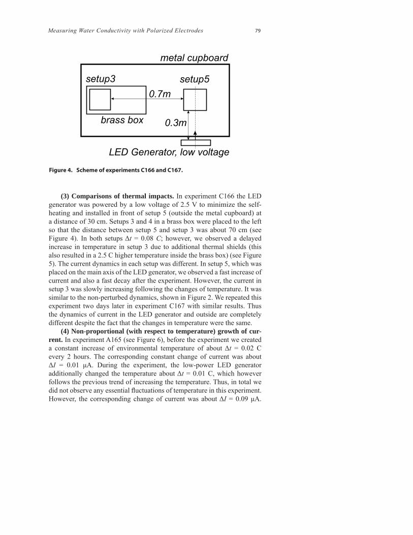
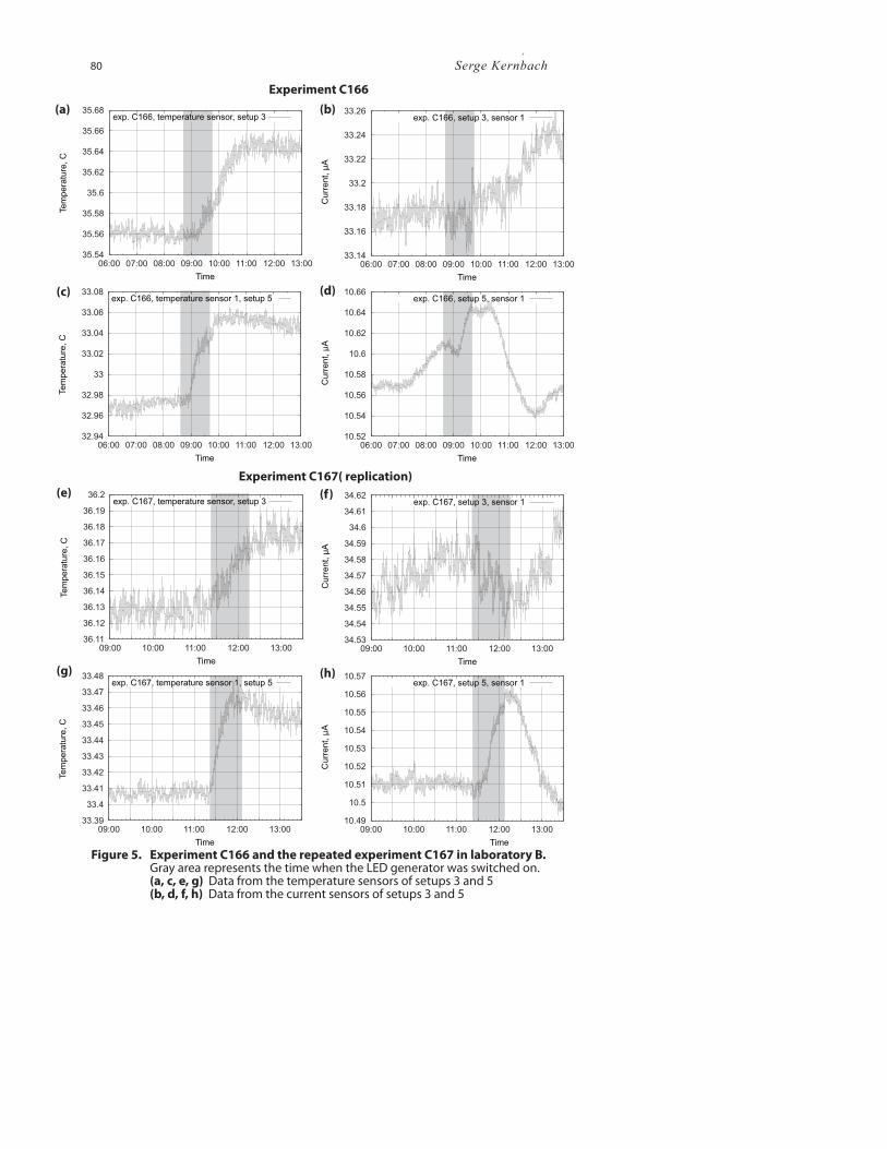
(3) Comparisons of thermal impacts. In experiment C166 the LED generator was powered by a low voltage of 2.5 V to minimize the self-heating and installed in front of setup 5 (outside the metal cupboard) at a distance of 30 cm. Setups 3 and 4 in a brass box were placed to the left so that the distance between setup 5 and setup 3 was about 70 cm (see Figure 4). In both setups Δt = 0.08 C; however, we observed a delayed increase in temperature in setup 3 due to additional thermal shields (this also resulted in a 2.5 C higher temperature inside the brass box) (see Figure 5). The current dynamics in each setup was different. In setup 5, which was placed on the main axis of the LED generator, we observed a fast increase of current and also a fast decay after the experiment. However, the current in setup 3 was slowly increasing following the changes of temperature. It was similar to the non-perturbed dynamics, shown in Figure 2. We repeated this experiment two days later in experiment C167 with similar results. Thus the dynamics of current in the LED generator and outside are completely different despite the fact that the changes in temperature were the same.

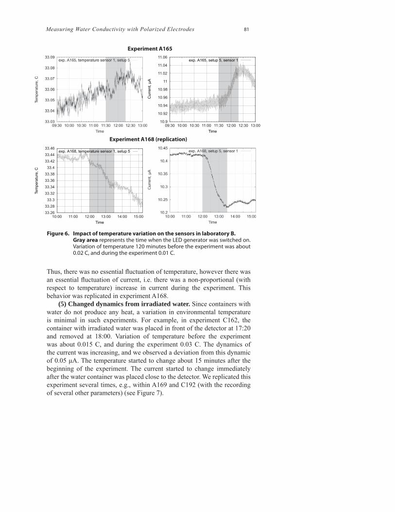
(4) Non-proportional (with respect to temperature) growth of cur-rent. In experiment A165 (see Figure 6), before the experiment we created a constant increase of environmental temperature of about Δt = 0.02 C every 2 hours. The corresponding constant change of current was about ΔI = 0.01 μA. During the experiment, the low-power LED generator additionally changed the temperature about Δt = 0.01 C, which however follows the previous trend of increasing the temperature. Thus, in total we did not observe any essential fl uctuations of temperature in this experiment. However, the corresponding change of current was about ΔI = 0.09 μA.

Figure 4. Scheme of experiments C166 and C167.

LED Generator, low voltage

metal cupboard

brass box

setup5

0.3m

0.7m

setup3

80 Serge Kernbach

Figure 5. Experiment C166 and the repeated experiment C167 in laboratory B. Gray area represents the time when the LED generator was switched on. (a, c, e, g) Data from the temperature sensors of setups 3 and 5 (b, d, f, h) Data from the current sensors of setups 3 and 5

35.54

35.56

35.58

35.6

35.62

35.64

35.66

35.68

06:00 07:00 08:00 09:00 10:00 11:00 12:00 13:00

Tem

pera

ture

, C

Time


33.14

33.16

33.18

33.2

33.22

33.24

33.26

06:00 07:00 08:00 09:00 10:00 11:00 12:00 13:00

Curr

ent, μ

A

Time


32.94

32.96

32.98

33

33.02

33.04

33.06

33.08

06:00 07:00 08:00 09:00 10:00 11:00 12:00 13:00

Tem

pera

ture

, C

Time

exp. C166, temperature sensor 1, setup 5

10.52

10.54

10.56

10.58

10.6

10.62

10.64

10.66

06:00 07:00 08:00 09:00 10:00 11:00 12:00 13:00

Curr

ent, μ

A

Time


36.11

36.12

36.13

36.14

36.15

36.16

36.17

36.18

36.19

36.2

09:00 10:00 11:00 12:00 13:00

Tem

pera

ture

, C

Time


34.53

34.54

34.55

34.56

34.57

34.58

34.59

34.6

34.61

34.62

09:00 10:00 11:00 12:00 13:00

Curr

ent, μ

A

Time


33.39

33.4

33.41

33.42

33.43

33.44

33.45

33.46

33.47

33.48

09:00 10:00 11:00 12:00 13:00

Tem

pera

ture

, C

Time


10.49

10.5

10.51

10.52

10.53

10.54

10.55

10.56

10.57

09:00 10:00 11:00 12:00 13:00

Curr

ent, μ

A

Time


(a) (b)

(c) (d)

(e) (f)

(g) (h)

Experiment C166

Experiment C167( replication)


Thus, there was no essential fl uctuation of temperature, however there was an essential fl uctuation of current, i.e. there was a non-proportional (with respect to temperature) increase in current during the experiment. This behavior was replicated in experiment A168.

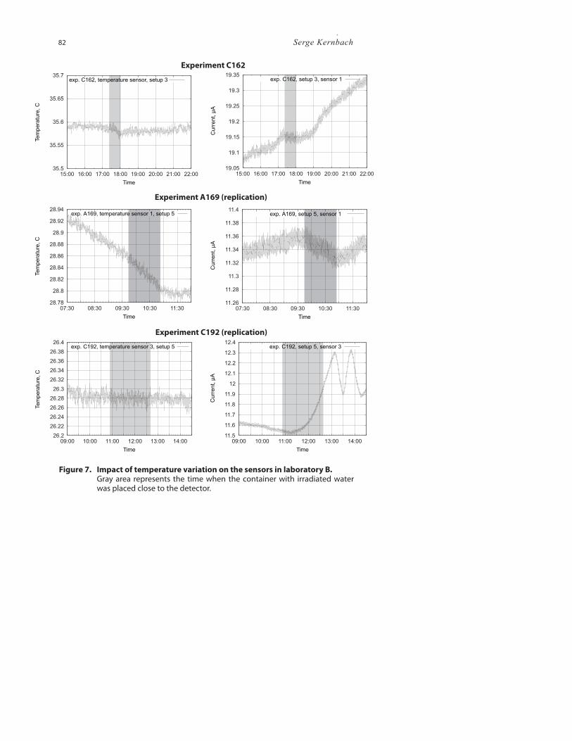
(5) Changed dynamics from irradiated water. Since containers with water do not produce any heat, a variation in environmental temperature is minimal in such experiments. For example, in experiment C162, the container with irradiated water was placed in front of the detector at 17:20 and removed at 18:00. Variation of temperature before the experiment was about 0.015 C, and during the experiment 0.03 C. The dynamics of the current was increasing, and we observed a deviation from this dynamic of 0.05 μA. The temperature started to change about 15 minutes after the beginning of the experiment. The current started to change immediately after the water container was placed close to the detector. We replicated this experiment several times, e.g., within A169 and C192 (with the recording of several other parameters) (see Figure 7).

Figure 6. Impact of temperature variation on the sensors in laboratory B. Gray area represents the time when the LED generator was switched on.

Variation of temperature 120 minutes before the experiment was about 0.02 C, and during the experiment 0.01 C.

10.9

10.92

10.94

10.96

10.98

11

11.02

11.04

11.06

09:30 10:00 10:30 11:00 11:30 12:00 12:30 13:00

Curr

ent, μ

A

Time


33.26

33.28

33.3

33.32

33.34

33.36

33.38

33.4

33.42

33.44

33.46

10:00 11:00 12:00 13:00 14:00 15:00

Tem

pera

ture

, C

Time

exp. A168, temperature sensor 1, setup 5

Experiment A168 (replication)

Experiment A165

82 Serge Kernbach

Figure 7. Impact of temperature variation on the sensors in laboratory B. Gray area represents the time when the container with irradiated water

was placed close to the detector.

35.5

35.55

35.6

35.65

35.7

15:00 16:00 17:00 18:00 19:00 20:00 21:00 22:00

Tem

pera

ture

, C

Time


19.05

19.1

19.15

19.2

19.25

19.3

19.35

15:00 16:00 17:00 18:00 19:00 20:00 21:00 22:00

Curr

ent, μ

A

Time


28.78

28.8

28.82

28.84

28.86

28.88

28.9

28.92

28.94

07:30 08:30 09:30 10:30 11:30

Tem

pera

ture

, C

Time

exp. A169, temperature sensor 1, setup 5

11.26

11.28

11.3

11.32

11.34

11.36

11.38

11.4

07:30 08:30 09:30 10:30 11:30

Curr

ent, μ

A

Time


26.2

26.22

26.24

26.26

26.28

26.3

26.32

26.34

26.36

26.38

26.4

09:00 10:00 11:00 12:00 13:00 14:00

Tem

pera

ture

, C

Time


11.5

11.6

11.7

11.8

11.9

12

12.1

12.2

12.3

12.4

09:00 10:00 11:00 12:00 13:00 14:00

Curr

ent, μ

A

Time


Experiment C162

Experiment A169 (replication)

Experiment C192 (replication)


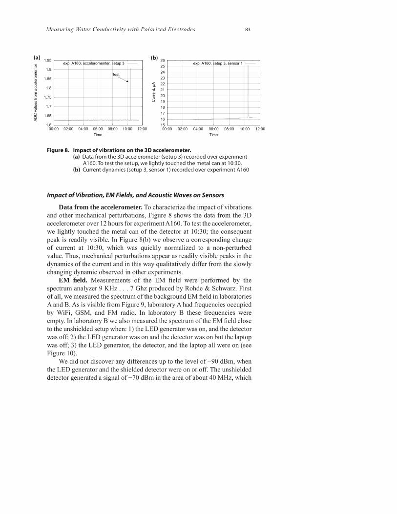
Figure 8. Impact of vibrations on the 3D accelerometer. (a) Data from the 3D accelerometer (setup 3) recorded over experiment A160. To test the setup, we lightly touched the metal can at 10:30. (b) Current dynamics (setup 3, sensor 1) recorded over experiment A160

1.6

1.65

1.7

1.75

1.8

1.85

1.9

1.95

00:00 02:00 04:00 06:00 08:00 10:00 12:00

AD

C v

alu

es fro

m a

ccele

rom

ente

r

Time

Test

exp. A160, acceleromenter, setup 3

15

16

17

18

19

20

21

22

23

24

25

26

00:00 02:00 04:00 06:00 08:00 10:00 12:00

Curr

ent, μ

A

Time


(a) (b)

Impact of Vibration, EM Fields, and Acoustic Waves on Sensors

Data from the accelerometer. To characterize the impact of vibrations and other mechanical perturbations, Figure 8 shows the data from the 3D accelerometer over 12 hours for experiment A160. To test the accelerometer, we lightly touched the metal can of the detector at 10:30; the consequent peak is readily visible. In Figure 8(b) we observe a corresponding change of current at 10:30, which was quickly normalized to a non-perturbed value. Thus, mechanical perturbations appear as readily visible peaks in the dynamics of the current and in this way qualitatively differ from the slowly changing dynamic observed in other experiments.

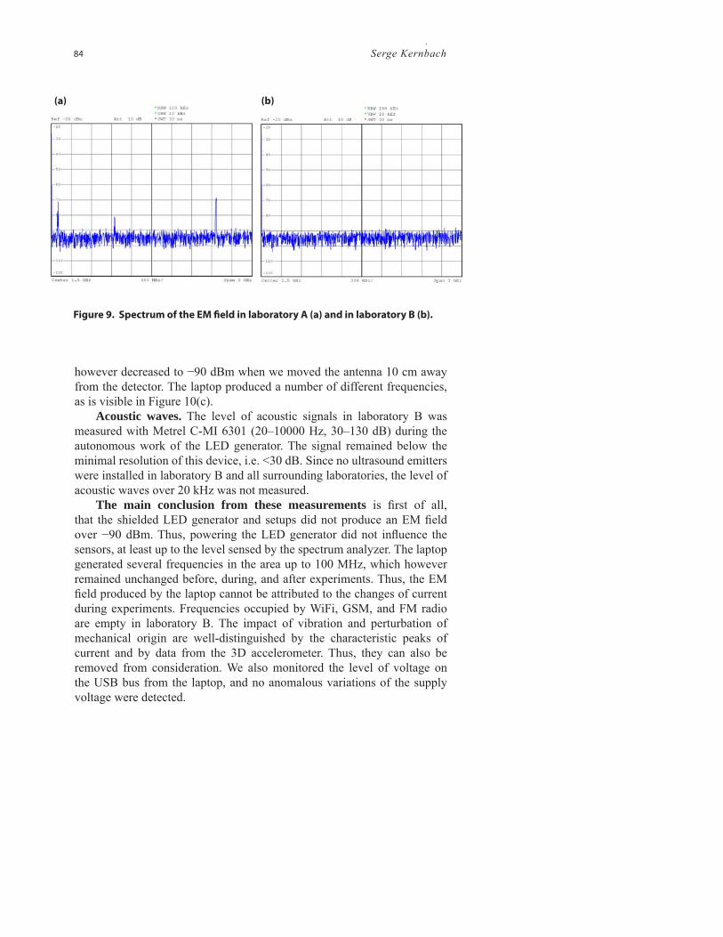
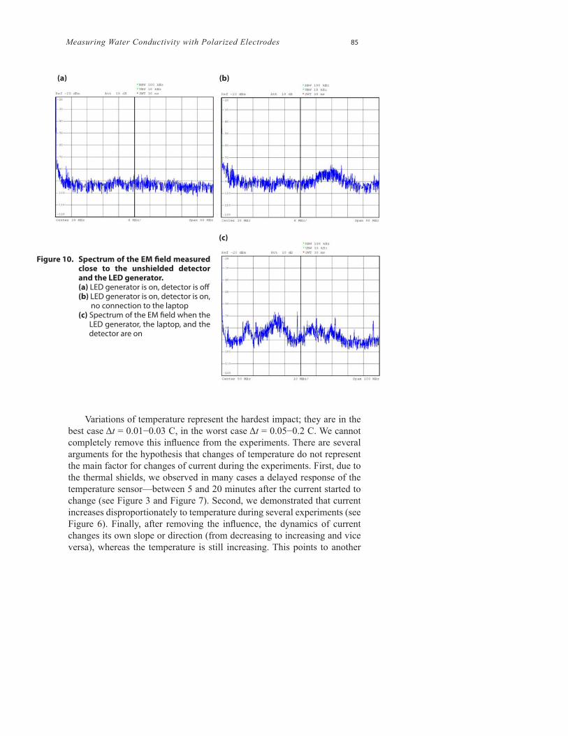
EM fi eld. Measurements of the EM fi eld were performed by the spectrum analyzer 9 KHz . . . 7 Ghz produced by Rohde & Schwarz. First of all, we measured the spectrum of the background EM fi eld in laboratories A and B. As is visible from Figure 9, laboratory A had frequencies occupied by WiFi, GSM, and FM radio. In laboratory B these frequencies were empty. In laboratory B we also measured the spectrum of the EM fi eld close to the unshielded setup when: 1) the LED generator was on, and the detector was off; 2) the LED generator was on and the detector was on but the laptop was off; 3) the LED generator, the detector, and the laptop all were on (see Figure 10).

We did not discover any differences up to the level of −90 dBm, when the LED generator and the shielded detector were on or off. The unshielded detector generated a signal of −70 dBm in the area of about 40 MHz, which

84 Serge Kernbach

Figure 9. Spectrum of the EM fi eld in laboratory A (a) and in laboratory B (b).

(a) (b)

however decreased to −90 dBm when we moved the antenna 10 cm away from the detector. The laptop produced a number of different frequencies, as is visible in Figure 10(c).

Acoustic waves. The level of acoustic signals in laboratory B was measured with Metrel C-MI 6301 (20–10000 Hz, 30–130 dB) during the autonomous work of the LED generator. The signal remained below the minimal resolution of this device, i.e. <30 dB. Since no ultrasound emitters were installed in laboratory B and all surrounding laboratories, the level of acoustic waves over 20 kHz was not measured.

The main conclusion from these measurements is fi rst of all, that the shielded LED generator and setups did not produce an EM fi eld over −90 dBm. Thus, powering the LED generator did not infl uence the sensors, at least up to the level sensed by the spectrum analyzer. The laptop generated several frequencies in the area up to 100 MHz, which however remained unchanged before, during, and after experiments. Thus, the EM fi eld produced by the laptop cannot be attributed to the changes of current during experiments. Frequencies occupied by WiFi, GSM, and FM radio are empty in laboratory B. The impact of vibration and perturbation of mechanical origin are well-distinguished by the characteristic peaks of current and by data from the 3D accelerometer. Thus, they can also be removed from consideration. We also monitored the level of voltage on the USB bus from the laptop, and no anomalous variations of the supply voltage were detected.


Figure 10. Spectrum of the EM fi eld measured close to the unshielded detector and the LED generator.

(a) LED generator is on, detector is off (b) LED generator is on, detector is on,

no connection to the laptop (c) Spectrum of the EM fi eld when the

LED generator, the laptop, and the detector are on

Variations of temperature represent the hardest impact; they are in the best case Δt = 0.01−0.03 C, in the worst case Δt = 0.05−0.2 C. We cannot completely remove this infl uence from the experiments. There are several arguments for the hypothesis that changes of temperature do not represent the main factor for changes of current during the experiments. First, due to the thermal shields, we observed in many cases a delayed response of the temperature sensor—between 5 and 20 minutes after the current started to change (see Figure 3 and Figure 7). Second, we demonstrated that current increases disproportionately to temperature during several experiments (see Figure 6). Finally, after removing the infl uence, the dynamics of current changes its own slope or direction (from decreasing to increasing and vice versa), whereas the temperature is still increasing. This points to another

(a) (b)

(c)

86 Serge Kernbach

factor (besides the variation in temperature) infl uencing the dynamics of the current.

Experiment Series C

Experiments with the LED Generator

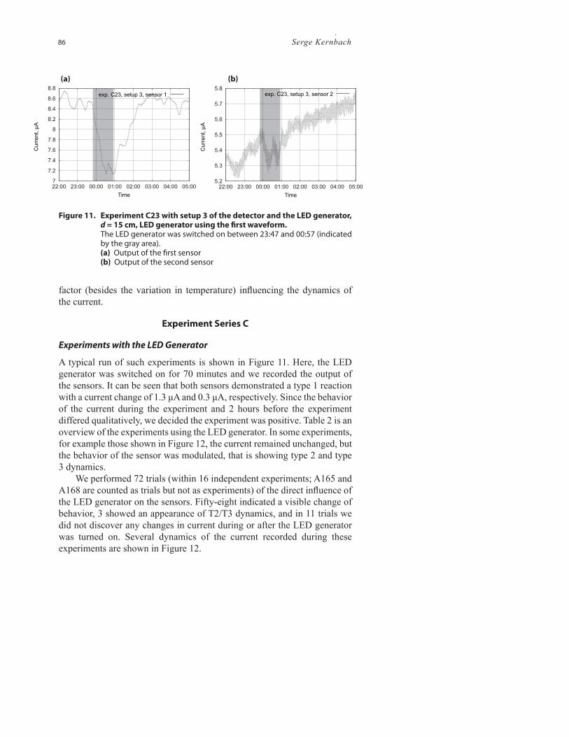
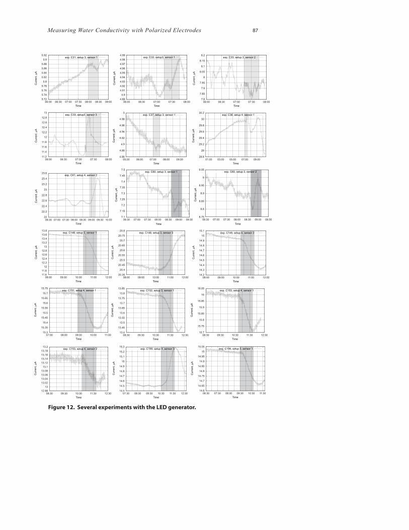
A typical run of such experiments is shown in Figure 11. Here, the LED generator was switched on for 70 minutes and we recorded the output of the sensors. It can be seen that both sensors demonstrated a type 1 reaction with a current change of 1.3 μA and 0.3 μA, respectively. Since the behavior of the current during the experiment and 2 hours before the experiment differed qualitatively, we decided the experiment was positive. Table 2 is an overview of the experiments using the LED generator. In some experiments, for example those shown in Figure 12, the current remained unchanged, but the behavior of the sensor was modulated, that is showing type 2 and type 3 dynamics.

We performed 72 trials (within 16 independent experiments; A165 and A168 are counted as trials but not as experiments) of the direct infl uence of the LED generator on the sensors. Fifty-eight indicated a visible change of behavior, 3 showed an appearance of T2/T3 dynamics, and in 11 trials we did not discover any changes in current during or after the LED generator was turned on. Several dynamics of the current recorded during these experiments are shown in Figure 12.

Figure 11. Experiment C23 with setup 3 of the detector and the LED generator, d = 15 cm, LED generator using the fi rst waveform.

The LED generator was switched on between 23:47 and 00:57 (indicated by the gray area).

(a) Output of the fi rst sensor (b) Output of the second sensor

7

7.2

7.4

7.6

7.8

8

8.2

8.4

8.6

8.8

22:00 23:00 00:00 01:00 02:00 03:00 04:00 05:00

Curr

ent, μ

A

Time


5.2

5.3

5.4

5.5

5.6

5.7

5.8

22:00 23:00 00:00 01:00 02:00 03:00 04:00 05:00

Curr

ent, μ

A

Time


(a) (b)


Figure 12. Several experiments with the LED generator.

5.72

5.74

5.76

5.78

5.8

5.82

5.84

5.86

5.88

5.9

5.92

06:00 06:30 07:00 07:30 08:00 08:30 09:00

Curr

ent, μ

A

Time


4.89

4.9

4.91

4.92

4.93

4.94

4.95

4.96

4.97

4.98

4.99

06:00 06:30 07:00 07:30 08:00

Curr

ent, μ

A

Time

exp. C33, setup3, sensor 1

7.8

7.85

7.9

7.95

8

8.05

8.1

8.15

8.2

06:00 06:30 07:00 07:30 08:00

Curr

ent, μ

A

Time


11.2

11.4

11.6

11.8

12

12.2

12.4

12.6

12.8

13

06:00 06:30 07:00 07:30 08:00

Curr

ent, μ

A

Time


4.86

4.88

4.9

4.92

4.94

4.96

4.98

5

05:00 06:00 07:00 08:00 09:00

Curr

ent, μ

A

Time


28.8

29

29.2

29.4

29.6

29.8

30

30.2

01:00 03:00 05:00 07:00 09:00

Curr

ent, μ

A

Time


22

22.2

22.4

22.6

22.8

23

23.2

23.4

23.6

06:30 07:00 07:30 08:00 08:30 09:00 09:30 10:00

Curr

ent, μ

A

Time


7.1

7.15

7.2

7.25

7.3

7.35

7.4

7.45

7.5

06:30 07:00 07:30 08:00 08:30 09:00 09:30


Curr

ent, μ

A

Time

8.75

8.8

8.85

8.9

8.95

9

9.05

06:30 07:00 07:30 08:00 08:30 09:00 09:30


Curr

ent, μ

A

Time

11.6

11.8

12

12.2

12.4

12.6

12.8

13

13.2

13.4

13.6

13.8

08:00 09:00 10:00 11:00 12:00

Curr

ent, μ

A

Time


20.35

20.4

20.45

20.5

20.55

20.6

20.65

20.7

20.75

20.8

08:00 09:00 10:00 11:00 12:00

Curr

ent, μ

A

Time


14.2

14.3

14.4

14.5

14.6

14.7

14.8

14.9

15

15.1

08:00 09:00 10:00 11:00 12:00

Curr

ent, μ

A

Time


15.3

15.35

15.4

15.45

15.5

15.55

15.6

15.65

15.7

15.75

07:00 08:00 09:00 10:00 11:00

Curr

ent, μ

A

Time


13.4

13.45

13.5

13.55

13.6

13.65

13.7

13.75

13.8

13.85

08:30 09:30 10:30 11:30 12:30

Curr

ent, μ

A

Time


15.7

15.75

15.8

15.85

15.9

15.95

16

16.05

08:30 09:30 10:30 11:30 12:30

Curr

ent, μ

A

Time


12.98

13

13.02

13.04

13.06

13.08

13.1

13.12

13.14

13.16

13.18

13.2

08:30 09:30 10:30 11:30 12:30

Curr

ent, μ

A

Time


14.4

14.5

14.6

14.7

14.8

14.9

15

15.1

15.2

15.3

07:30 08:30 09:30 10:30 11:30 12:30

Curr

ent, μ

A

Time


14.6

14.65

14.7

14.75

14.8

14.85

14.9

14.95

15

15.05

06:30 07:30 08:30 09:30 10:30 11:30

Curr

ent, μ

A

Time


88 Serge Kernbach

TABLE 2

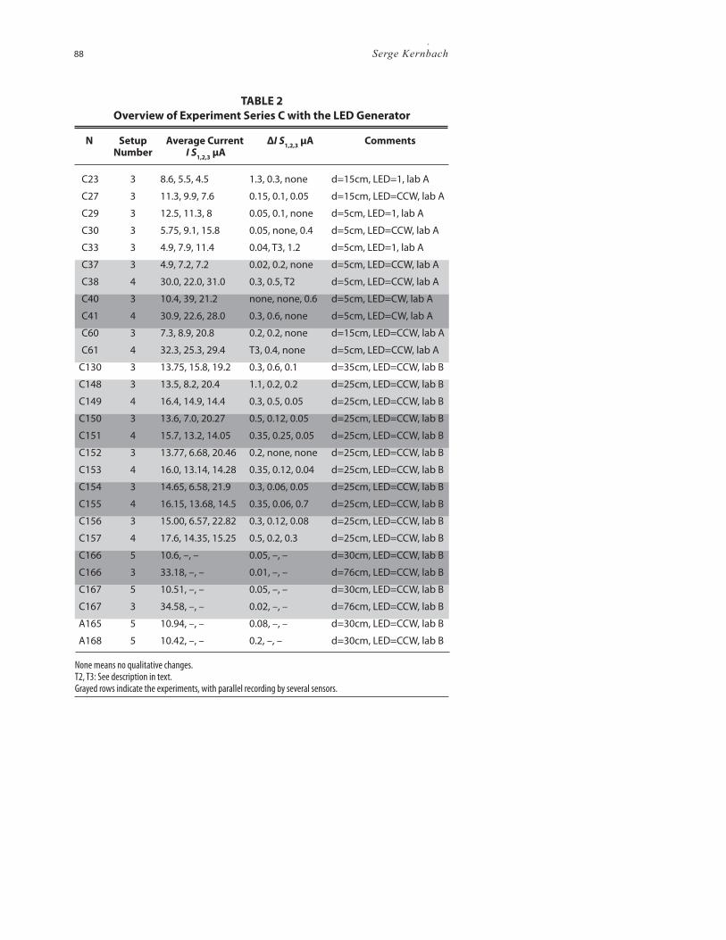
Overview of Experiment Series C with the LED Generator

N SetupNumber

Average Current I S

1,2,3 μA

ΔI S1,2,3

μA Comments

C23 3 8.6, 5.5, 4.5 1.3, 0.3, none d=15cm, LED=1, lab A

C27 3 11.3, 9.9, 7.6 0.15, 0.1, 0.05 d=15cm, LED=CCW, lab A

C29 3 12.5, 11.3, 8 0.05, 0.1, none d=5cm, LED=1, lab A

C30 3 5.75, 9.1, 15.8 0.05, none, 0.4 d=5cm, LED=CCW, lab A

C33 3 4.9, 7.9, 11.4 0.04, T3, 1.2 d=5cm, LED=1, lab A

C37 3 4.9, 7.2, 7.2 0.02, 0.2, none d=5cm, LED=CCW, lab A

C38 4 30.0, 22.0, 31.0 0.3, 0.5, T2 d=5cm, LED=CCW, lab A

C40 3 10.4, 39, 21.2 none, none, 0.6 d=5cm, LED=CW, lab A

C41 4 30.9, 22.6, 28.0 0.3, 0.6, none d=5cm, LED=CW, lab A

C60 3 7.3, 8.9, 20.8 0.2, 0.2, none d=15cm, LED=CCW, lab A

C61 4 32.3, 25.3, 29.4 T3, 0.4, none d=5cm, LED=CCW, lab A

C130 3 13.75, 15.8, 19.2 0.3, 0.6, 0.1 d=35cm, LED=CCW, lab B

C148 3 13.5, 8.2, 20.4 1.1, 0.2, 0.2 d=25cm, LED=CCW, lab B

C149 4 16.4, 14.9, 14.4 0.3, 0.5, 0.05 d=25cm, LED=CCW, lab B

C150 3 13.6, 7.0, 20.27 0.5, 0.12, 0.05 d=25cm, LED=CCW, lab B

C151 4 15.7, 13.2, 14.05 0.35, 0.25, 0.05 d=25cm, LED=CCW, lab B

C152 3 13.77, 6.68, 20.46 0.2, none, none d=25cm, LED=CCW, lab B

C153 4 16.0, 13.14, 14.28 0.35, 0.12, 0.04 d=25cm, LED=CCW, lab B

C154 3 14.65, 6.58, 21.9 0.3, 0.06, 0.05 d=25cm, LED=CCW, lab B

C155 4 16.15, 13.68, 14.5 0.35, 0.06, 0.7 d=25cm, LED=CCW, lab B

C156 3 15.00, 6.57, 22.82 0.3, 0.12, 0.08 d=25cm, LED=CCW, lab B

C157 4 17.6, 14.35, 15.25 0.5, 0.2, 0.3 d=25cm, LED=CCW, lab B

C166 5 10.6, –, – 0.05, –, – d=30cm, LED=CCW, lab B

C166 3 33.18, –, – 0.01, –, – d=76cm, LED=CCW, lab B

C167 5 10.51, –, – 0.05, –, – d=30cm, LED=CCW, lab B

C167 3 34.58, –, – 0.02, –, – d=76cm, LED=CCW, lab B

A165 5 10.94, –, – 0.08, –, – d=30cm, LED=CCW, lab B

A168 5 10.42, –, – 0.2, –, – d=30cm, LED=CCW, lab B

None means no qualitative changes.T2, T3: See description in text.Grayed rows indicate the experiments, with parallel recording by several sensors.


Experiments with Irradiated Water

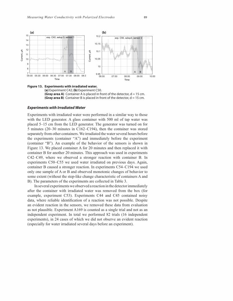
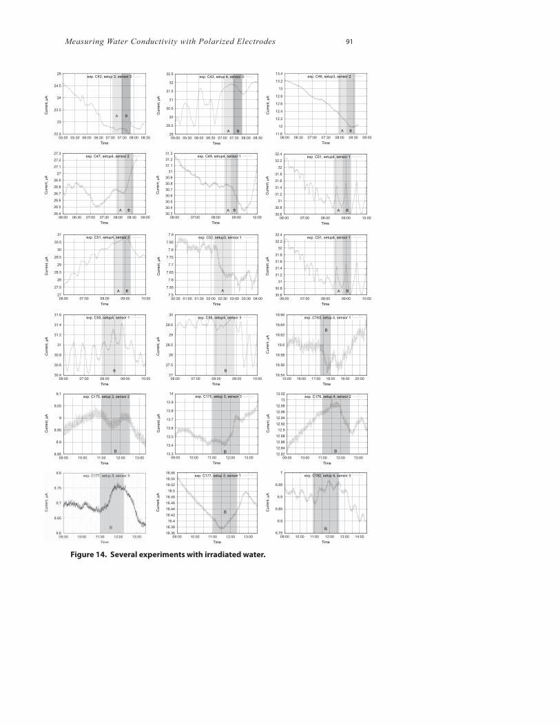
Experiments with irradiated water were performed in a similar way to those with the LED generator. A glass container with 500 ml of tap water was placed 5–15 cm from the LED generator. The generator was turned on for 5 minutes (20–30 minutes in C162–C194), then the container was stored separately from other containers. We irradiated the water several hours before the experiments (container “A”) and immediately before the experiment (container “B”). An example of the behavior of the sensors is shown in Figure 13. We placed container A for 20 minutes and then replaced it with container B for another 20 minutes. This approach was used in experiments C42–C49, where we observed a stronger reaction with container B. In experiments C50–C55 we used water irradiated on previous days. Again, container B caused a stronger reaction. In experiments C54–C194 we used only one sample of A or B and observed monotonic changes of behavior to some extent (without the step-like change characteristic of containers A and B). The parameters of the experiments are collected in Table 3.

In several experiments we observed a reaction in the detector immediately after the container with irradiated water was removed from the box (for example, experiment C53). Experiments C44 and C45 contained noisy data, where reliable identifi cation of a reaction was not possible. Despite an evident reaction in the sensors, we removed these data from evaluation as not plausible. Experiment A169 is counted as a single trial and not as an independent experiment. In total we performed 82 trials (16 independent experiments), in 24 cases of which we did not observe an evident reaction (especially for water irradiated several days before an experiment).

Figure 13. Experiments with irradiated water. (a) Experiment C42; (b) Experiment C50. (Gray area A) Container A is placed in front of the detector, d = 15 cm. (Gray area B) Container B is placed in front of the detector, d = 15 cm.

7

8

9

10

11

12

13

14

15

05:00 05:30 06:00 06:30 07:00 07:30 08:00 08:3

Curr

ent, μ

A

Time


A B BA9.95

10

10.05

10.1

10.15

10.2

06:00 07:00 08:00 09:00 10:00

Curr

ent, μ

A

Time


(a) (b)

90 Serge Kernbach

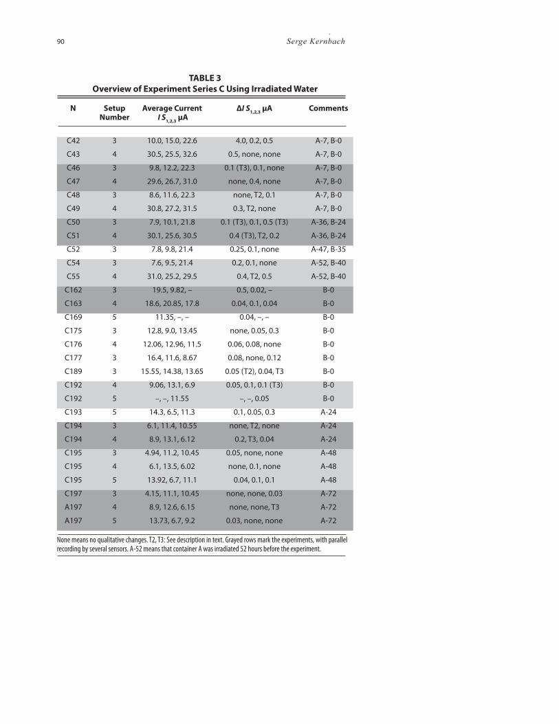
TABLE 3

Overview of Experiment Series C Using Irradiated Water

N SetupNumber

Average Current I S

1,2,3 μA

ΔI S1,2,3

μA Comments

C42 3 10.0, 15.0, 22.6 4.0, 0.2, 0.5 A-7, B-0

C43 4 30.5, 25.5, 32.6 0.5, none, none A-7, B-0

C46 3 9.8, 12.2, 22.3 0.1 (T3), 0.1, none A-7, B-0

C47 4 29.6, 26.7, 31.0 none, 0.4, none A-7, B-0

C48 3 8.6, 11.6, 22.3 none, T2, 0.1 A-7, B-0

C49 4 30.8, 27.2, 31.5 0.3, T2, none A-7, B-0

C50 3 7.9, 10.1, 21.8 0.1 (T3), 0.1, 0.5 (T3) A-36, B-24

C51 4 30.1, 25.6, 30.5 0.4 (T3), T2, 0.2 A-36, B-24

C52 3 7.8, 9.8, 21.4 0.25, 0.1, none A-47, B-35

C54 3 7.6, 9.5, 21.4 0.2, 0.1, none A-52, B-40

C55 4 31.0, 25.2, 29.5 0.4, T2, 0.5 A-52, B-40

C162 3 19.5, 9.82, – 0.5, 0.02, – B-0

C163 4 18.6, 20.85, 17.8 0.04, 0.1, 0.04 B-0

C169 5 11.35, –, – 0.04, –, – B-0

C175 3 12.8, 9.0, 13.45 none, 0.05, 0.3 B-0

C176 4 12.06, 12.96, 11.5 0.06, 0.08, none B-0

C177 3 16.4, 11.6, 8.67 0.08, none, 0.12 B-0

C189 3 15.55, 14.38, 13.65 0.05 (T2), 0.04, T3 B-0

C192 4 9.06, 13.1, 6.9 0.05, 0.1, 0.1 (T3) B-0

C192 5 –, –, 11.55 –, –, 0.05 B-0

C193 5 14.3, 6.5, 11.3 0.1, 0.05, 0.3 A-24

C194 3 6.1, 11.4, 10.55 none, T2, none A-24

C194 4 8.9, 13.1, 6.12 0.2, T3, 0.04 A-24

C195 3 4.94, 11.2, 10.45 0.05, none, none A-48

C195 4 6.1, 13.5, 6.02 none, 0.1, none A-48

C195 5 13.92, 6.7, 11.1 0.04, 0.1, 0.1 A-48

C197 3 4.15, 11.1, 10.45 none, none, 0.03 A-72

A197 4 8.9, 12.6, 6.15 none, none, T3 A-72

A197 5 13.73, 6.7, 9.2 0.03, none, none A-72

None means no qualitative changes. T2, T3: See description in text. Grayed rows mark the experiments, with parallel recording by several sensors. A-52 means that container A was irradiated 52 hours before the experiment.


Figure 14. Several experiments with irradiated water.

22.5

23

23.5

24

24.5

25

05:00 05:30 06:00 06:30 07:00 07:30 08:00 08:30

Curr

ent, μ

A

Time


A B

29

29.5

30

30.5

31

31.5

32

32.5

05:00 05:30 06:00 06:30 07:00 07:30 08:00 08:30

Curr

ent, μ

A

Time

A B


A B11.8

12

12.2

12.4

12.6

12.8

13

13.2

13.4

06:00 06:30 07:00 07:30 08:00 08:30 09:00

Curr

ent, μ

A

Time


A B26.4

26.5

26.6

26.7

26.8

26.9

27

27.1

27.2

27.3

06:00 06:30 07:00 07:30 08:00 08:30 09:00

Curr

ent, μ

A

Time


30.3

30.4

30.5

30.6

30.7

30.8

30.9

31

31.1

31.2

31.3

06:00 07:00 08:00 09:00 10:00

Curr

ent, μ

A

Time

A B


BA30.6

30.8

31

31.2

31.4

31.6

31.8

32

32.2

32.4

06:00 07:00 08:00 09:00 10:00

Curr

ent, μ

A

Time


BA27

27.5

28

28.5

29

29.5

30

30.5

31

06:00 07:00 08:00 09:00 10:00

Curr

ent, μ

A

Time


7.5

7.55

7.6

7.65

7.7

7.75

7.8

7.85

7.9

00:30 01:00 01:30 02:00 02:30 03:00 03:30 04:00

Curr

ent, μ

A

Time

A


BA30.6

30.8

31

31.2

31.4

31.6

31.8

32

32.2

32.4

06:00 07:00 08:00 09:00 10:00

Curr

ent, μ

A

Time


B

30.4

30.6

30.8

31

31.2

31.4

31.6

06:00 07:00 08:00 09:00 10:00

Curr

ent, μ

A

Time


B

27

27.5

28

28.5

29

29.5

30

06:00 07:00 08:00 09:00 10:00

Curr

ent, μ

A

Time


18.54

18.56

18.58

18.6

18.62

18.64

18.66

15:00 16:00 17:00 18:00 19:00 20:00

Curr

ent, μ

A

Time


B

8.85

8.9

8.95

9

9.05

9.1

09:00 10:00 11:00 12:00 13:00

Curr

ent, μ

A

Time


B13.3

13.4

13.5

13.6

13.7

13.8

13.9

14

09:00 10:00 11:00 12:00 13:00

Curr

ent, μ

A

Time


B12.82

12.84

12.86

12.88

12.9

12.92

12.94

12.96

12.98

13

13.02

09:00 10:00 11:00 12:00 13:00

Curr

ent, μ

A

Time


B

16.36

16.38

16.4

16.42

16.44

16.46

16.48

16.5

16.52

16.54

16.56

09:00 10:00 11:00 12:00 13:00

Curr

ent, μ

A

Time


B

6.75

6.8

6.85

6.9

6.95

7

09:00 10:00 11:00 12:00 13:00 14:00

Curr

ent, μ

A

Time


B

92 Serge Kernbach

Control Experiments

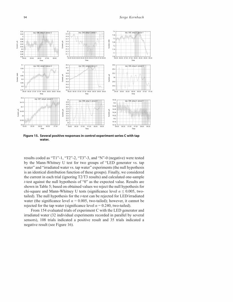
The control experiments were carried out under the same conditions as experiment series C; however, we used normal tap water. A container with water was rested 12 hours in the laboratory, then installed 15 cm in front of the detectors and exposed for between 30 minutes and 90 minutes. In several experiments (C62, C63, C199) the container remained in the laboratory for several days before an experiment. An overview of the control experiments is shown in Table 4. The reaction of the sensors in these experiments is signifi cantly weaker than in the previous ones. For instance, we observed a type 1 reaction with step-like changes of current, as shown for example in Figure 13 and Figure 11. From 79 trials (of 14 independent experiments) we obtained 63 negative and only 8 positive reactions. It should be noted that in the original experiments with irradiated water (Bobrov 2009) the authors also obtained reactions in the sensors in control experiments that were weaker than the reactions with the irradiated water. The dynamics of the current in several positive cases are shown in Figure 15. Based on the criteria for previous experiments, we qualifi ed several results from these experiments as positive. Within the boundaries of these experiments, we cannot identify whether these were caused by environmental noise or whether there were other pertinent factors, for instance a long resting time in the laboratory.

Discussion of Results

An overview of all experiments is given in Table 5. Since negative results are evaluated as results without any change in current, with a change of less than 0.01 μA, including where the parameters of the oscillations changed, there is doubt whether this was caused by irradiation or whether this oscillation has multiple frequencies. We excluded four datasets from the evaluation in which the sensors demonstrated a signifi cant change of current before or after the experiment, or where the data were not plausible due to noise from the environment. If two or more sensors in a series C experiment were simultaneously positive, that experiment was counted as positive.

Evaluating the experiments we performed, we can conclude that all independent experiments with the LED generator and the irradiated water are positive. Most of the experiments with the tap water are negative (except those where the tap water was rested for several days in the laboratory). We performed several statistical tests for the trials. First of all, positive trials are coded as “1”, negative trials as “0” (i.e. trials are considered as experiments with binary output, T2/T3 results are not counted), and then we ran the chi-square goodness of fi t test against the null hypothesis of the random character of the obtained data. Second, the


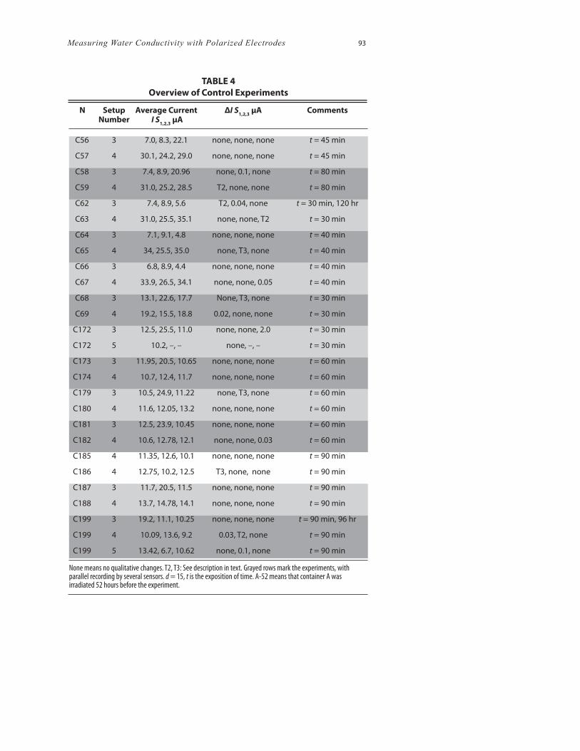
TABLE 4

Overview of Control Experiments

N SetupNumber

Average Current I S

1,2,3 μA

ΔI S1,2,3

μA Comments

C56 3 7.0, 8.3, 22.1 none, none, none t = 45 min


C58 3 7.4, 8.9, 20.96 none, 0.1, none t = 80 min

C59 4 31.0, 25.2, 28.5 T2, none, none t = 80 min

C62 3 7.4, 8.9, 5.6 T2, 0.04, none t = 30 min, 120 hr

C63 4 31.0, 25.5, 35.1 none, none, T2 t = 30 min


C65 4 34, 25.5, 35.0 none, T3, none t = 40 min


C67 4 33.9, 26.5, 34.1 none, none, 0.05 t = 40 min

C68 3 13.1, 22.6, 17.7 None, T3, none t = 30 min

C69 4 19.2, 15.5, 18.8 0.02, none, none t = 30 min

C172 3 12.5, 25.5, 11.0 none, none, 2.0 t = 30 min

C172 5 10.2, –, – none, –, – t = 30 min



C179 3 10.5, 24.9, 11.22 none, T3, none t = 60 min



C182 4 10.6, 12.78, 12.1 none, none, 0.03 t = 60 min


C186 4 12.75, 10.2, 12.5 T3, none, none t = 90 min



C199 3 19.2, 11.1, 10.25 none, none, none t = 90 min, 96 hr

C199 4 10.09, 13.6, 9.2 0.03, T2, none t = 90 min

C199 5 13.42, 6.7, 10.62 none, 0.1, none t = 90 min

None means no qualitative changes. T2, T3: See description in text. Grayed rows mark the experiments, with parallel recording by several sensors. d = 15, t is the exposition of time. A-52 means that container A was irradiated 52 hours before the experiment.

94 Serge Kernbach

Figure 15. Several positive responses in control experiment series C with tap water.

8.84

8.86

8.88

8.9

8.92

8.94

8.96

8.98

9

9.02

9.04

04:00 05:00 06:00 07:00 08:00

Curr

ent, μ

A

Time


31

31.1

31.2

31.3

31.4

31.5

31.6

31.7

31.8

31.9

32

04:00 04:30 05:00 05:30 06:00 06:30 07:00 07:30 08:00

Curr

ent, μ

A

Time


7.05

7.1

7.15

7.2

7.25

7.3

7.35

7.4

06:00 06:30 07:00 07:30 08:00 08:30 09:00 09:30

Curr

ent, m

kA

Time


8.75

8.8

8.85

8.9

8.95

9

9.05

9.1

06:00 06:30 07:00 07:30 08:00 08:30 09:00 09:30

Curr

ent, m

kA

Time


34.3

34.4

34.5

34.6

34.7

34.8

34.9

35

35.1

35.2

06:00 06:30 07:00 07:30 08:00 08:30 09:00 09:30

Curr

ent, μ

A

Time


24.4

24.6

24.8

25

25.2

25.4

25.6

04:30 05:00 05:30 06:00 06:30 07:00 07:30

Curr

ent, μ

A

Time


33.9

33.95

34

34.05

34.1

34.15

34.2

05:00 05:30 06:00 06:30 07:00


Curr

ent, μ

A

Time

21.9

22

22.1

22.2

22.3

22.4

22.5

22.6

22.7

22.8

22.9

23

06:00 06:30 07:00 07:30 08:00 08:30

Curr

ent, μ

A

Time


19.16

19.18

19.2

19.22

19.24

19.26

19.28

19.3

19.32

06:00 06:30 07:00 07:30 08:00 08:30

Curr

ent, μ

A

Time


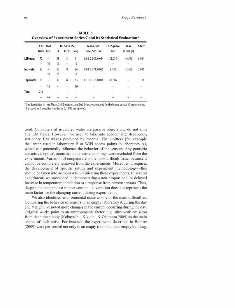
results coded as “T1”-1, “T2”-2, “T3”-3, and “N”-0 (negative) were tested by the Mann-Whitney U test for two groups of “LED generator vs. tap water” and “irradiated water vs. tap water” experiments (the null hypothesis is an identical distribution function of these groups). Finally, we considered the current in each trial (ignoring T2/T3 results) and calculated one-sample t-test against the null hypothesis of “0” as the expected value. Results are shown in Table 5; based on obtained values we reject the null hypothesis for chi-square and Mann-Whitney U tests (signifi cance level α ≤ 0.005, two-tailed). The null hypothesis for the t-test can be rejected for LED/irradiated water (the signifi cance level α = 0.005, two-tailed); however, it cannot be rejected for the tap water (signifi cance level α = 0.240, two-tailed).

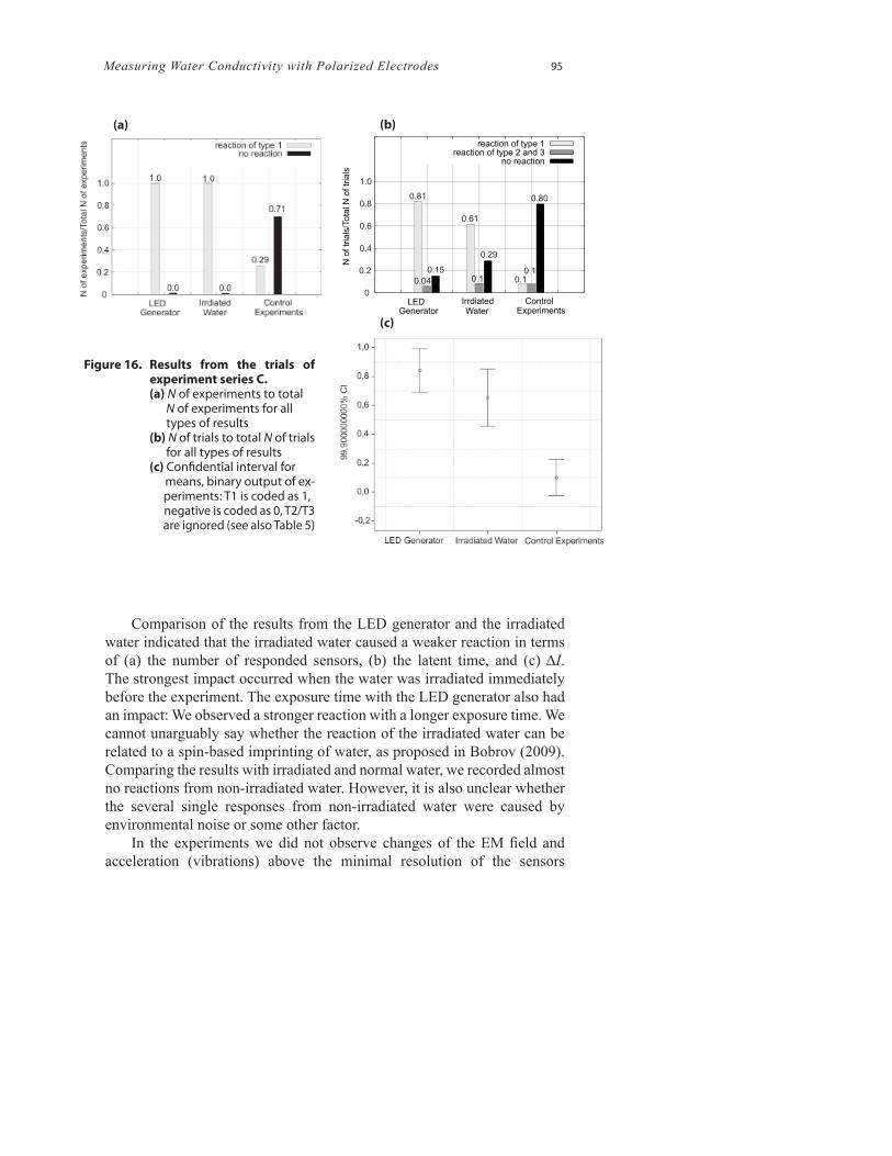
From 154 evaluated trials of experiment C with the LED generator and irradiated water (32 individual experiments recorded in parallel by several sensors), 108 trials indicated a positive result and 35 trials indicated a negative result (see Figure 16).


Figure 16. Results from the trials of experiment series C.

(a) N of experiments to total N of experiments for all types of results (b) N of trials to total N of trials for all types of results (c) Confi dential interval for means, binary output of experiments: T1 is coded as 1, negative is coded as 0, T2/T3

are ignored (see also Table 5)

LED IrrdiatedWaterGenerator Experiments

Control0

0.2

0.4

0.6

0.80.81

0.61

0.80

0.29

0.150.1

0.1

1.0

N o

f tr

ials

/Tota

l N

of tr

ials

reaction of type 1reaction of type 2 and 3

no reaction

0.04 0.1

(a) (b)

(c)

Comparison of the results from the LED generator and the irradiated water indicated that the irradiated water caused a weaker reaction in terms of (a) the number of responded sensors, (b) the latent time, and (c) ΔI. The strongest impact occurred when the water was irradiated immediately before the experiment. The exposure time with the LED generator also had an impact: We observed a stronger reaction with a longer exposure time. We cannot unarguably say whether the reaction of the irradiated water can be related to a spin-based imprinting of water, as proposed in Bobrov (2009). Comparing the results with irradiated and normal water, we recorded almost no reactions from non-irradiated water. However, it is also unclear whether the several single responses from non-irradiated water were caused by environmental noise or some other factor.

In the experiments we did not observe changes of the EM fi eld and acceleration (vibrations) above the minimal resolution of the sensors

96 Serge Kernbach

used. Containers of irradiated water are passive objects and do not emit any EM fi elds. However, we need to take into account high-frequency, stationary EM waves produced by external EM emitters (for example the laptop used in laboratory B or WiFi access points in laboratory A), which can potentially infl uence the behavior of the sensors. Any parasitic capacitive, optical, acoustic, and electric couplings were excluded from the experiments. Variation of temperature is the most diffi cult issue, because it cannot be completely removed from the experiments. Moreover, it requires the development of specifi c setups and experiment methodology—this should be taken into account when replicating these experiments. In several experiments we succeeded in demonstrating a non-proportional or delayed increase in temperature in relation to a response from current sensors. Thus, despite the temperature-impact sensors, its variation does not represent the main factor for the changing current during experiments.

We also identifi ed environmental noise as one of the main diffi culties. Comparing the behavior of sensors in an empty laboratory A during the day and at night, we noted more changes in the current occurring during the day. Original works point to an anthropogenic factor, e.g., ultraweak emission from the human body (Kobayashi, Kikuchi, & Okamura 2009) as the main source of such noise. For instance, the experiments described in Bobrov (2009) were performed not only in an empty room but in an empty building.

TABLE 5

Overview of Experiment Series C and Its Statistical Evaluation*

N of N of RESULTS Mean, Std. Chi-Square M-W t-Test

Trials Exp. T1 T2/T3 Neg. Dev., Std. Err. Test U-Test (z)

LED gen. 72 – 58 3 11 0.84, 0.369, 0.044 32.014 −6.596 6.914

– 16 16 – 0 – – – –

Irr. water 82 – 50 8 24 0.68, 0.471, 0.055 9.135 −5.468 3.041

– 16 16 – 0 – – – –

Tap water 79 – 8 8 63 0.11, 0.318, 0.038 42.606 – 1.184

– 14 4 – 10 – – – –

Total 233 – – – – – – – –

– 46 – – – – – – –

* See description in text. Mean, Std. Deviation, and Std. Error are calculated for the binary output of experiments.T1 is coded as 1, negative is coded as 0, T2/T3 are ignored.


Thus, more robust experiments need to be performed in a special physical laboratory, where temperature, EM, and environmental and anthropogenic infl uences can be minimized by several orders of magnitude.

In brief, excluding EM, temperature, mechanical, optical, capacitive, and acoustic interactions, and any parasitic couplings, the publications cited mention two possible explanations for this behavior. First, Bobrov (2009, 2006) points to spin waves, which have been recently polemicized in the physics community. Experiments carried out with rotating objects, sources of radioactivity, and plant and animal cells support this theory to some extent and possibly explain interactions between biological and non-biological objects. Original publications suppose that spin waves generated by LEDs (or by the 630 nm helium–neon laser) are in charge of a spatial polarization of water dipoles in the Gouy–Chapman layer. Second, Zenin (2000) introduced stable macroclusters of water dipoles, which can exist for a long time (Zenin 2005). For instance, the behavior of a

inV on voltage electrodes in setup 2 (see Figure 21) can be explained by the appearance of such macroclusters of dipoles. Since sensors contain water, macroclusters of dipoles can infl uence conductivity and thus the current. In turn, the combination of different weak signals can affect the behavior of macroclusters. However, as mentioned in the Introduction, the goal of this work is only to replicate the cited experiments without deep physical or chemical discussions explaining the behavior of the sensors.

Conclusion

In several experiments we observed a causal dependency between switching on the LED generator or installing the water container and the reactions of the sensors. Between two and six sensors simultaneously recorded such reactions. The recorded data were evaluated about two hours before and after the experiments. The active LED generator and passive irradiated water caused a similar impact on the detectors, whereas tap water and a normal state (night hours without any objects close by) indicated mostly a monotonic dynamic in the sensors. The impact of such infl uences as temperature, EM fi elds, and others was minimized up to the level sensed by the measuring devices. Based on these results, we evaluate the main part of the replication attempt as successful.

We offer several notes regarding these experiments. First, the measured level of current is about 1−50 μA with a resolution of 0.01 μA. Measuring such a small current is sensitive to many factors: resistance of cables, input impedance of operational amplifi ers, temperature drift of electronic components, and electronic noise. Thus, while the setup has the advantage of compactness, it can only be used to detect changes. It is not intended for

98 Serge Kernbach

precise measurement of ionic processes appearing in the electric double layer. Second, the setup is protected from mechanical, optical, capacitive, temperature, and EM infl uences only up to the level allowed in a normal electronic laboratory. To improve the level of protection, for example when investigating the effect of very small infl uences, the experiments would have to be repeated in a special laboratory. We also did not investigate physico–chemical properties of water before and after experiments; these tests should be performed in such a laboratory. Third, we did not explore the impact of the geometrical placement of sensors and LED generator/water in all experiments, however it is assumed that such an impact exists and that the obtained results are infl uenced by it.

In the context of our research, the interaction between blue-light LEDs and deeply polarized electrodes introduces a new component in underwater communication. We observed this behavior in our original experiments. After performing experiment series C, this dependency became clearer. Since electric double layers are generally sensitive to mechanical and EM infl uences, it is possible that strong light or even the movement of mobile devices can be used to modulate an electric fi eld. This suggests future work.

Acknowledgment

We are very grateful to A.V. Bobrov for many suggestions on designing the experiment setup, performing the experiments, and evaluating the results.

References

Belaya, M. L., Feigel’man, M. V., & Levadnyii, V. G. (1987). Structural forces as a result of nonlocal water polarizability. Langmuir, 3(5), 648–654.

Bobrov, A. V. (1992). Investigating the mechanism of non-specifi c perception. In Современые проблемы изучения и сохранения биосферы, (Volume 2). pp. N2223–В2001, М. 2001 УДК: 577.38 + 612.014.

Bobrov, A. V. (1998). Experimental substantiation of the possible mechanism of laser therapy. In Electronic Instrument Engineering Proceedings, APEIE-98 (Volume 1), 4th International Conference on Actual Problems of EIE. pp. 175–78.

Bobrov, A. V. (2002). Биологические И Физические Свойства Активированной Воды [Biological and Physical Properties of Activated Water]. IEEE Proceedings 2282.

Bobrov, A. V. (2006). Investigating a Field Concept of Consciousness [Модельное Исследование Полевой Концепции Механизма Сознания]. Orel, Russia: Orel State Technical University.

Bobrov, A. V. (2009). Interaction between spin fi elds of material objects. In Материалы международной научной конференции; Khosta, Russia; August 25–29, 2009. pp. 76–86.

Bristow, K. L., Kluitenberg, G. J., Goding, C. J., & Fitzgerald, T. S. (2001). A small multi-needle probe for measuring soil thermal properties, water content, and electrical conductivity. Computers and Electronics in Agriculture, 31(3), 265–280.


David, W., Gruen, R., & Marcelja, S. (1983). Spatially varying polarization in water. A model for the electric double layer and the hydration force. Journal of the Chemical Society, Faraday Transactions 2, 79, 225–242.

Dipper, T., Gebhardt, K., Kernbach, S., & von der Emde, G. (2011). Investigating the behaviour of weakly electric fi sh with a fi sh avatar. In International Workshop on Bio-inspired Robots.

von der Emde, G., Schwarz, S., Gomez, L. Budelli, R., & Grant, K. (1998). Electric fi sh measure distance in the dark. Nature, 395, 890–894.

Kernbach, S., Dipper, T., & Sutantyo, D. (2011). Multi-modal local sensing and communication for collective underwater systems. In Proceedings of the 11th International Conference on Mobile Robots and Competitions, ROBOTICA 11. pp. 96–101.

Kirkham, D., & Taylor, G. S. (1949). Some tests of a four-electrode probe for soil moisture measurement. Proceedings, Soil Science Society of America 14, 42–46.

Kobayashi, M., Kikuchi, D., & Okamura, H. (2009). Imaging of ultraweak spontaneous photon emission from the human body displaying diurnal rhythm. PLoS ONE, 4(7), 6256.

Kornyshev, A. A. (2007). Double-layer in ionic liquids: A paradigm change? The Journal of Physical Chemistry B, 111(20), 5545–5557. PMID: 17469864.

Kumar, R., & Skinner, J. L. (2008). Water simulation model with explicit three-molecule interactions. The Journal of Physical Chemistry B, 112(28), 8311–8318. PMID: 18570461.

Lyklema, J. (2005). Fundamentals of Interface and Colloid Science. Academic Press.Muzalewskay, N. I., & Bobrov, А. V. (1988). On a possible role of the electrical double layer in the

reaction of biological objects to external infl uences. Биофизика [Biophysics], 33(4), 725. Orion Conductivity Theory, Orion Products—The Technical Edge. Technical report. http://www.thermo.com/eThermo/CMA/PDFs/Articles/articlesFile_11377.pdfOtt, H. (1988). Noise Reduction Techniques in Electronic Systems. New York: John Wiley & Sons.Parker, G. W. (2002). Electric fi eld outside a parallel plate capacitor. American Journal of Physics,

70(5), 502. Rai, D., Kulkarni, A. D., Gejji, S. P., & Pathak, R. K. (2008). Water clusters (H2On, n = 6–8) in external

electric fi elds. The Journal of Chemical Physics, 128(3), 034310.Schmickl, T., Thenius, R., Moslinger, C., Timmis, J., Tyrell, A. Read, M. Hilder, J. Halloy, J. Campo,

A., Stefanini, C., Manfredi, L., Orofi no, S. Kernbach, S., Dipper, T., & Sutantyo, D. (2011). Self-Adaptive and Self-Organizing Systems Workshops (SASOW). In Proceedings of the Fifth IEEE Conference on The Self-Aware Underwater Swarm, October 2011, pp. 120-126. doi 10.1109/SASOW.2011.11

Sim, M., & Kim, D. (2011). Electrolocation with an electric organ discharge waveform for biomimetic application. Adaptive Behavior, 19(3), 172–186.

Spillner, F. (1957). Vier-elektroden-konduktometrische analyse (4-ek-analyse). Chemie Ingenieur Technik, 29(1), 24–27.

Stenschke, H. (1985). Polarization of water in the metal/electrolyte interface. Journal of Electroanalytical Chemistry and Interfacial Electrochemistry, 196(2), 261–274.

Vegiri, A., & Schevkunov, S. V. (2001). A molecular dynamics study of structural transitions in small water clusters in the presence of an external electric fi eld. The Journal of Chemical Physics, 115(9), 4175–4185.

Zenin, S. (2000). Scientifi c Foundation and Application Problems of Energo-Information Interactions in Nature [Научные основы и прикладные проблемы энергоинформацион-ных взаимодействий в природе и обществе]. Мoscow: Russian State Library.

Zenin, S. (2005). Structured State of Water as a Basis for Monitoring of Living Systems [Структурированное состояние воды как основа управления по-ведением и безопасностью живых систем]. Moscow: Russian State Library.

100 Serge Kernbach

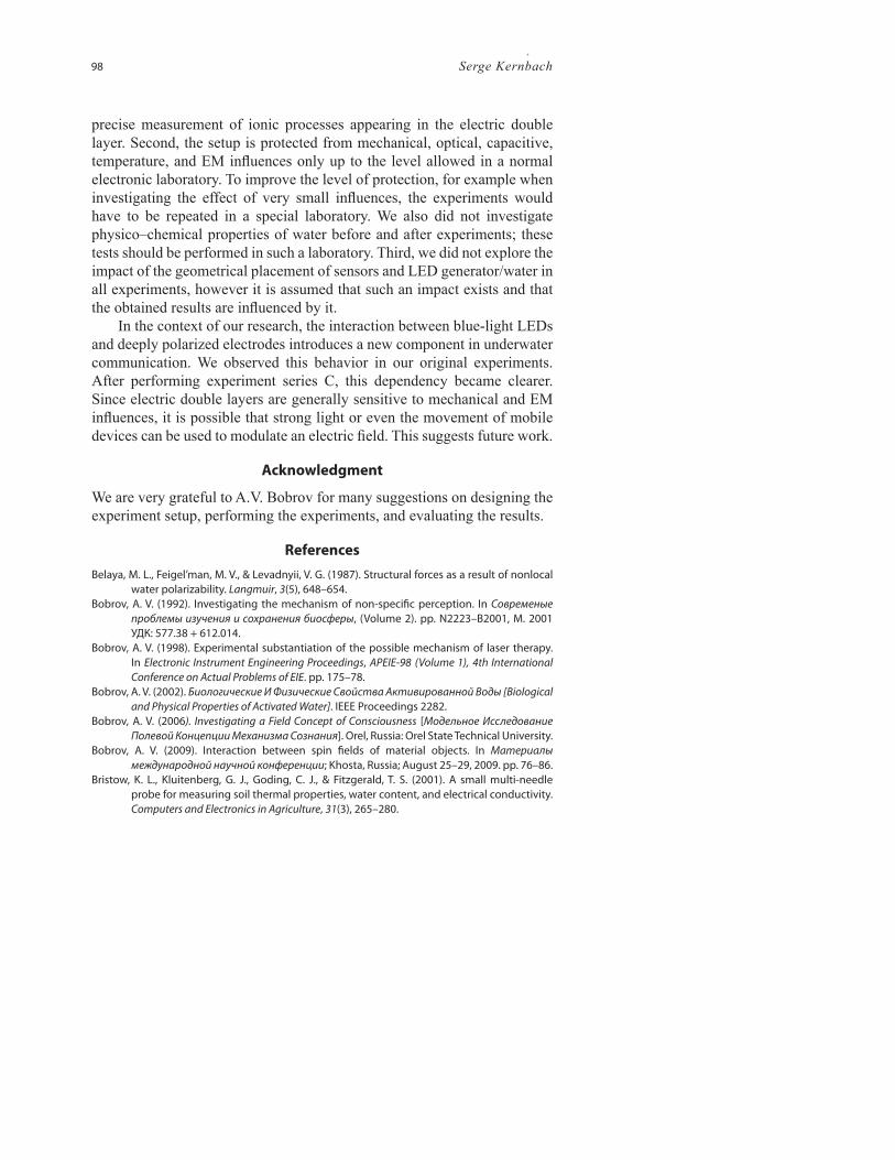
Appendix AExperiment Setup

The original experiments (Bobrov 2009) used DC voltage up to 30 V. For the replication experiments we used the well-known four-electrode scheme (see Figure 17). The electrodes Vout take their voltage from a digital–analog converter (DAC) in the range of ±5 V. The current fl owing in the DAC circuit is converted to a voltage and digitalized by an analog–digital converter (ADC). The voltage from Vin electrodes is amplifi ed by an operational amplifi er and also digitalized by an ADC. Both the DAC and ADC are connected to the microcontroller. Data are transmitted via a USB interface to a laptop and sampled at a frequency of 1 Hz in real time (each measurement from the ADC is time-stamped). We used two versions of this equipment. The fi rst version has an instrumental operational amplifi er (AD8226), external DAC (AD5322), and ADC (AD7656), and provides an accuracy of current and voltage measurement of μA and mV ranges of 0.1%.

The second version uses a programmable system on chip (PSoC)

Figure 17. Structural scheme of the experiment setup. Voltage electrodes are installed only in setups 2 and 3.

OpAmp

Vout

Vin

Vin

Vout current to

temperature

converter

voltage

3D accelerometer

ADC

DAC

USB

microcontroller

PSoC 5 CY8CKIT-014

I

V

I

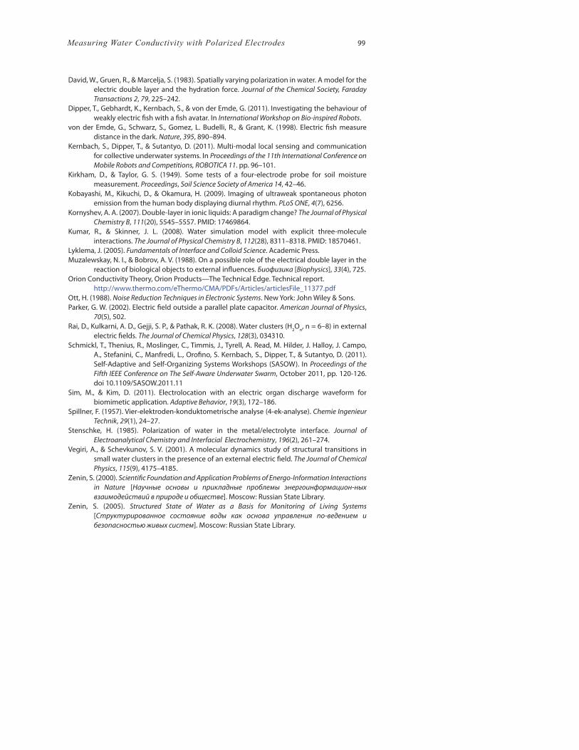
Figure 18. Noise produced by the DAC and power supply.


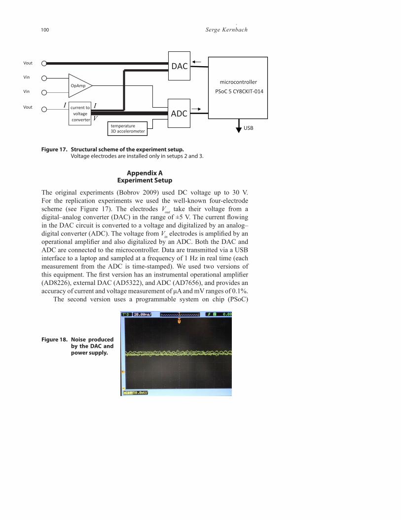
Figure 19. Description of the experiment setups. (a) Setup 1, with a 1000 ml glass bottle containing a plastic tube of 3 cm diameter. The electrodes are made of copper (in the form of a ring) and installed on the plastic tube, distance between electrodes as shown. The glass bottle is closed by a plastic cover, with the electrodes inside. (b) Setup 2 uses 300 ml water with 8 electrodes made from stainless steel of 1 mm diameter. (c) Setup 3 has 3 independent sets of electrodes made from stainless steel of 1 mm diameter. Corresponding containers are glass jars of about 50 ml. (d) Setup 4 has 3 independent sets of electrodes. The anode is a 1 mm wire, the cathode is a cylinder, both electrodes are made from stainless steel.

Vout

Vin

8cm5cm

Vin

Vout

24mm

12mm

V

V

V

V

V

V

b

b

a

a

out

out

in

in

in

in

86mm

o= mm36

58mm

Vout

Vout

(a) (b)

(c) (d)

CY8C5588AXI 060 with internal amplifi ers, DAC, and ADC. Accuracy of measurement is about 3%. The system is powered at 5 V through a USB interface from a laptop. The noise from the DAC and power supply is shown in Figure 18 and is in the range ±10 mV, about 0.3% of the voltage generated. To reduce the level of noise, a software fi lter averages values

102 Serge Kernbach

from the ADC (current and voltage) within a sliding frame of fi ve steps.The electronics also contain a 3D accelerometer KXSC7-2050

(sensitivity 660 mV/g) and three types of temperature sensors: NCP21XV103J03RA (installed on PCB), LM35AH, and AD592CNZ (installed in the containers with electrodes). The sensitivity of temperature measurement is below 0.01 C with a 20-bit ADC. Setups 3, 4, and 5 have two, two, and four temperature sensors, respectively. Data from temperature, acceleration sensors, and voltage of power supply were recorded during all the experiments to demonstrate the infl uence of these factors. For calibration and test measurements, an Agilent Technology oscilloscope DSO1014A and true RMS Multimeter 72-7730 for accurate DC current measurement in the range ±(0.1% + 15) were used.

All setups were shielded in a similar manner. All sensors from setups 3 and 4 were fi rst inserted into metal cans made of 0.5 mm steel (three sensors in each) (see Figure 1), and then both cans were placed into a box made from 1 mm brass. Each sensor from setup 5 was inserted into a pipe made of 3 mm brass. All metal cans, boxes, and pipe were grounded. Temperature shields were experimentally selected from several materials. First we used boxes made of 80-mm–thick styrofoam; however, it seems this material is not suitable for experiments. Finally, all metal containers were lined with 10-mm rubber matting and empty space was fi lled up with wool.

Since the fi rst setup remained from our previous experiments and had copper electrodes, it was removed from further tests. All other electrodes were made from chromium–nickel stainless steel (setups 2, 3, 4) and platinum (setup 5) of 1 mm diameter. Setup 5 is similar to setup 3, only the electrodes are made of platinum and they can be shifted inside a glass container. In all setups we used deionized water produced by Walter Schmidt Chemie GmbH (osmosis approach) and double-distilled water produced by AuxynHairol.

The LED generator is shown in Figure 20. It consists of 169 blue-light (470 nm) LEDs LC503FBL1-15Q-A3 placed in an area 120 × 120 mm2. These have a luminous intensity of 11 cd and opening angle of 15 degrees. The LED generator has eight switchable fi elds and is controlled by an ATMega328 microcontroller. Powering of the digital part and LEDs is independent for each, and the voltage applied to LEDs can be varied within 2.5–6 V. In other experiments with deeply polarized electrodes, we applied up to 48 V to LEDs—we have experimental evidence that LEDs with a higher voltage impact more intensively on sensors. The microcontroller has a temperature sensor. For experiments without an operator, the microcontroller monitors the environmental temperature and can autonomously start an experiment when the variation of temperature is


Figure 20. The LED generator. (a) Structure of the LED generator (b) LED generator made with 169 blue-light (470 nm) LEDs (c) LED generator: rotation of sectors CCW and CW

Powersupply0-6V

8x independentN MOSFETSTS2DNF30L

LEDsegments 1-8

LDO 3V,XC6206

UARTinterface to PC

microcontrollerATMega328

temperaturesensor

...

...

(a)

(b) (c)

rotation CW

rotation CCW

low (there is a log of all activities of the LED generator). We programmed four modes of operation: oscillation 1 (LED = 1, “on” pulse—1 μs, “off”—333 μs), oscillation 2 (LED = 2, “on” pulse—100 ms, “off”—100 ms), and rotation of sectors CCW and CW (LED = CCW, CW, “on” pulse—100 ms, “off”—100 ms) (see Figure 20(c)). To avoid parasitic coupling, the LED generator ran on two, three, or four D-size batteries.

104 Serge Kernbach

Loss of sensitivity. After a while, sensors lose their sensitivity. This loss shows when the current quickly stabilizes to a particular value and does not indicate even normal environmental noise. This effect was confi rmed by A.V. Bobrov for his sensors. The timeframe within which a sensor loses sensitivity varies between a few days and a few weeks. We surmised that contamination of the electrodes was the reason for this effect; when it appeared, we replaced all the electrodes and changed the water. Sensors are also less sensitive when they relax after disturbances or after powering the systems. Usually, we waited for 6–8 hours after powering before operating the sensors. After disturbances, the relaxation time is between 3 and 12 hours. Loss of sensitivity could be one of the reasons why, in several experiments, some sensors did not record any changes of current, whereas other sensors did.

Voltage in ainV and b

inV electrodes. In the second and third setups we used a

inV and binV electrodes to test the hypothesis that macroclusters

of water dipoles were created (Zenin 2000). The idea is inspired by Orion Conductivity Theory (no date), in which a “current position” ( b

inV ) and a “fi eld position” ( a

inV ) in the four-electrode scheme are distinguished. Analyzing the state of the art in this area, we discovered a number of works (Vegiri & Schevkunov 2001, Rai, Kulkarni, Gejji, & Pathak 2008) concerning the clustering of water in electric fi elds as well as the simulation of clustering behavior (Kumar & Skinner 2008). Based on these works, we anticipated different potential dynamics of a

inV and binV electrodes. This

was experimentally confi rmed, for instance in Figure 21 we plot ainV and

binV in two particular experiments. It can be seen that the potential for a

inV can change its polarity (the polarity of Vout remained constant); artefacts on

Figure 21. “Current position” vs. “fi eld position”. (a) Experiment A10 (b) Experiment A15

(a) (b)


Figure 22. DAC current, “fi eld position,” and “current position”.

See description in the text. Dynamics of the current

in the DAC circuit (a), and the voltage on b

inV in the electrodes (b) and on a

inV in the electrodes (c) are shown.

30

30.2

30.4

30.6

30.8

31

31.2

31.4

08:00 08:30 09:00 09:30 10:00

Curr

ent, μ

A

Time

0.006

0.008

0.01

0.012

0.014

0.016

0.018

0.02

0.022

0.024

08:00 08:30 09:00 09:30 10:00

Voltage, V

Time

Voltage on V electrodesb

in

0.3665

0.367

0.3675

0.368

0.3685

0.369

0.3695

0.37

0.3705

08:00 08:30 09:00 09:30 10:00

Voltage, V

Time

Voltage on V electrodesa

in

(a) (b)

(c)

one set of electrodes were not observed on other sets of electrodes. In the preliminary experiments with the LED generator (discussed in the section Experiment Series C) we recorded the dynamics a

inV and binV and the

current in the DAC circuit, as shown in Figure 22.We can see that a

inV demonstrates similar dynamics on the current, that is the voltage of the four- and six-electrode schemes are also sensitive to non-EM fi elds. Since these experiments move away from the original approach (Bobrov 2006), we decided to postpone them and, for this work, concentrate on current detection. In setups 3, 4, and 5 we analyzed only the current fl owing through the DAC circuit.

Auto-oscillation mode. As mentioned in Bobrov (2009, 2006), sensors can enter a so-called “auto-oscillation” mode. The period of these oscillations varies between a few minutes and a few hours. We are unable to estimate the current range in which the auto-oscillation can appear. We observed the spontaneous start of oscillations between 4 and 40 μA, that is, in the whole range of current measurement. Bobrov (2006) suggested that this mode is more sensitive to non-EM fi elds.

Documents

Measuring Water Conductivity with Polarized Electrodes