1

27th

June 2015 PJH

Tutorial on CellML, OpenCOR & the Physiome Model Repository

This tutorial shows you how to install and run the OpenCOR1 software [1], to author and edit CellML

models2 [2] and to use the Physiome Model Repository (PMR)

3 [3]. We start by giving a brief

background on the VPH-Physiome project. We then create a simple model, save it as a CellML file

and run model simulations. We next try opening existing CellML models, both from a local directory

and from the Physiome Model Repository. The various features of CellML4 and OpenCOR are then

explained in the context of increasingly complex biological models. A simple linear first order ODE

model and a nonlinear third order model are introduced. Ion channel gating models are used to

introduce the way that CellML handles units, components, encapsulation groups and connections.

More complex potassium and sodium ion channel models are then developed and subsequently

imported into the Hodgkin-Huxley 1952 squid axon neural model using the CellML model import

facility. The Noble 1962 model of a cardiac cell action potential is used to illustrate importing of units

and parameters. The tutorial finishes with sections on model annotation and the facilities available

on the CellML website and the Physiome Model Repository to support model development,

including the links to bioinformatic databases. There is a strong emphasis in the tutorial on

establishing ‘best practice’ in the creation of CellML models and using the PMR resources,

particularly in relation to modular approaches (model hierarchies) and model annotation.

Note: This tutorial relies on readers having some background in algebra and calculus, but tries to

explain all mathematical concepts beyond this, along with the physical principles, as they are needed

for the development of CellML models.5

Contents page 1. Background to the VPH-Physiome project ..................................................................................... 2

2. Install and launch OpenCOR ............................................................................................................ 3

3. Create and run a simple CellML model: editing and simulation ..................................................... 4

4. Open an existing CellML file from a local directory or the Physiome Model Repository ............... 8

5. A simple first order ODE ................................................................................................................. 9

6. The Lorenz attractor ..................................................................................................................... 10

7. A model of ion channel gating and current: Introducing CellML units ........................................ 12

8. A model of the potassium channel: Introducing CellML components and connections ............. 16

9. A model of the sodium channel: Introducing CellML encapsulation and interfaces ................... 20

10. A model of the nerve action potential: Introducing CellML imports ........................................... 24

11. A model of the cardiac action potential: Importing units and parameters ................................. 28

12. Model annotation ......................................................................................................................... 34

13. The Physiome Model Repository and the link to bioinformatics ................................................. 38

14. Speed comparisons with MATLAB ................................................................................................ 42

15. SED-ML, functional curation and Web Lab .................................................................................. 43

16. Future developments ................................................................................................................... 44

17. References .................................................................................................................................... 45

1 OpenCOR is an open source, freely available, C

++ desktop application written by Alan Garny at INRIA with

funding support from the Auckland Bioengineering Institute (www.abi.auckland.ac.nz) and the NIH-funded

Virtual Physiological Rat (VPR) project led by Dan Beard at the University of Michigan (http://virtualrat.org). 2 For an overview and the background of CellML see www.cellml.org. This project is led by Poul Nielsen and

David (Andre) Nickerson at the Auckland (University) Bioengineering Institute (ABI: www.abi.auckland.ac.nz). 3 https://models.physiomeproject.org. The PMR project is led by Tommy Yu at the ABI.

4 For details on the specifications of CellML1.0 see www.cellml.org/specifications/cellml_1.0.

5 Please send any errors discovered or suggested improvements to p.hunter@auckland.ac.nz.

MedTech CoRE

2

1. Background to the VPH-Physiome project

To be of benefit to applications in healthcare, organ and whole organism

physiology needs to be understood at both a systems level and in terms of

subcellular function and tissue properties. Understanding a re-entrant

arrhythmia in the heart, for example, depends on knowledge of not only

numerous cellular ionic current mechanisms and signal transduction

pathways, but also larger scale myocardial tissue structure and the spatial

variation in protein expression. As reductionist biomedical science succeeds

in elucidating ever more detail at the molecular level, it is increasingly

difficult for physiologists to relate integrated whole organ function to

underlying biophysically detailed mechanisms that exploit this molecular

knowledge. Multi-scale computational modelling is used by engineers and

physicists to design and analyse mechanical, electrical and chemical

engineering systems. Similar approaches could benefit the understanding of

physiological systems. To address these challenges and to take advantage

of bioengineering approaches to modelling anatomy and physiology, the

International Union of Physiological Sciences (IUPS) formed the Physiome

Project in 1997 as an international collaboration to provide a computational

framework for understanding human physiology6.

One of the primary goals of the Physiome Project [4] has been to promote

the development of standards for the exchange of information between

models. The first of these standards, dealing with time varying but spatially

lumped processes, is CellML [5]. The second (dealing with spatially and time

varying processes) is FieldML [6,7]7. A further goal of the Physiome Project

has been the development of open source tools for creating and visualizing

standards-based models and running model simulations. OpenCOR is the

latest in a series of software projects aimed at providing a modelling

environment for CellML models. Similar tools exist for FieldML models.

Following the publication of the STEP8 (Strategy for a European Physiome)

Roadmap in 2006, the European Commission in 2007 initiated the Virtual

Physiological Human (VPH) project [8]. A related US initiative by the

Interagency Modeling and Analysis Group (IMAG) began in 20039. These

projects and similar initiatives are now coordinated and are collectively

referred to here as the ‘VPH-Physiome’ project10. The VPH-Institute

11 was

formed in 2012 as a virtual organisation to providing strategic leadership,

initially in Europe but now globally, for the VPH-Physiome Project.

6 www.iups.org. The IUPS President, Denis Noble from Oxford University, and Jim Bassingthwaighte from the University of

Washington in Seattle have been two of the driving forces behind the Physiome Project. Peter Hunter from the University

of Auckland was appointed Chair of the newly created Physiome Commission of the IUPS in 2000. The IUPS Physiome

Committee, formed in 2008, was co-chaired by Peter Hunter and Sasha Popel (JHU) and is now chaired by Andrew

McCulloch from UCSD. The UK Wellcome Trust provided initial support for the Physiome Project through the Heart

Physiome grant awarded in 2004 to David Paterson, Denis Noble and Peter Hunter. 7 CellML began as a joint public-private initiative in 1998 with funding by the US company Physiome Sciences (CEO Jeremy

Levin), before being launched under IUPS as a fully open source project in 1999. 8 The STEP report, led by Marco Viceconte (University of Sheffield, UK), is available at www.europhysiome.org/roadmap.

9 This coordinates various US Governmental funding agencies involved in multi-scale bioengineering modeling research

including NIH, NSF, NASA, the Dept of Energy (DoE), the Dept of Defense (DoD), the US Dept of Agriculture and the Dept of

Veteran Affairs. See www.nibib.nih.gov/Research/MultiScaleModeling/IMAG. Grace Peng of NHBIB leads the IMAG group. 10

Other significant contributions to the VPH-Physiome project have come from Yoshi Kurachi in Japan (www.physiome.jp),

Stig Omholt in Norway (www.ntnu) and Chae-Hun Leem in Korea (www.physiome.or.kr). 11

www.vph-institute.org. Formed in 2012, the inaugural Director was Marco Viceconti. The current Director is Adriano

Henney. The inaugural and current President of the VPH-Institute is Denis Noble.

VPH-Institute

3

2. Install and launch OpenCOR

Download OpenCOR from www.opencor.ws. Versions are available for Windows, Mac and Linux.

Note that the annotation section of this tutorial relies on the OpenCOR snapshot 2015-06-09 (or

later). Create a shortcut to the executable (found in the bin directory) on your desktop and click on

this to launch OpenCOR. A window will appear that looks like Figure 1(a).

(a) (b)

Figure 1. (a) Default positioning of dockable windows. (b) An alternative configuration achieved by dragging

and dropping the dockable windows.

The central area is used to interact with files. By default, no files are open, hence the OpenCOR logo

is shown instead. To the sides, there are dockable windows, which provide additional features.

Those windows can be dragged and dropped to the top or bottom of the central area as shown in

Figure 1(b) or they can be individually undocked or closed. All closed panels can be re-displayed by

enabling them in the View menu, or by using the Tools menu Reset All option. Clicking on ‘CTRL’12 &

‘spacebar’ on the Windows version, removes (for less clutter) or restores these two side panels.

Any of the subpanels (Physiome Model Repository, File Browser, and File Organiser) can be closed

with the top right delete button, and then restored from the View .. Windows.. menu. Files can be

dragged and dropped into the File Organiser to create a local directory structure for your files.

OpenCOR has a plugin architecture

and can be used with or without a

range of modules. These can be

viewed under the Tools menu. By

default they are all included, as

shown in Figure 2. Information

about developing plugins for

OpenCOR is also available13

.

12

The ⌘ key being the equivalent on Macs. 13

www.opencor.ws/developer/develop/plugins/index.html

Figure 2. Showing the plugins for

OpenCOR that are selectable. Untick

the box on the bottom left to show all

plugins.

4

3. Create and run a simple CellML model: editing and simulation

In this example we create a simple CellML model and run it. The model is the Van der Pol oscillator14

defined by the second order equation

( )

with initial conditions . The parameter controls the magnitude of the damping

term. To create a CellML model we convert this to two first order equations15

by defining the

velocity

as a new variable :

( )

The initial conditions are now .

With the central pane in Editing mode (e.g. CellML Text view), under the File menu and New, click on

CellML 1.1 File then type in the following lines of code after deleting the three lines that indicate

where the code should go:

def model van_der_pol_model as

def comp main as

var t: dimensionless {init: 0}; var x: dimensionless {init: -2}; var y: dimensionless {init: 0}; var mu: dimensionless {init: 1};

// These are the ODEs

ode(x,t)=y;

ode(y,t)=mu*(1{dimensionless}-sqr(x))*y-x;

enddef; enddef;

Things to note16

are: (i) the closing semicolon at the end of each line (apart from the first two def statements that are opening a CellML construct); (ii) the need to indicate dimensions for each

variable and constant (all dimensionless in this example – but more on dimensions later); (iii) the use

of ode(x,t) to indicate a first order17

ODE in x and t, (iv) the use of the squaring function sqr(x) for ,

and (v) the use of ‘//’ to indicate a comment.

A partial list of mathematical functions available for OpenCOR is:

sqr(x) √ sqrt(x) ln(x) log(x) exp(x) pow(x,a)

sin(x) cos(x) tan(x) csc(x) sec(x) cot(x)

asin(x) acos(x) atan(x) acsc(x) asec(x) acot(x)

sinh(x) cosh(x) tanh(x) csch(x) sech(x) coth(x)

asinh(x) acosh(x) atanh(x) acsch(x) asech(x) acoth(x)

Table 1. The list of mathematical functions available for coding in OpenCOR.

Positioning the cursor over either of the ODEs renders the maths in standard form above the code as

shown in Figure 3(a).

14

en.wikipedia.org/wiki/Van_der_Pol_oscillator 15

Note that gray boxes are used to indicate equations that are implemented directly in OpenCOR. 16

For more on the CellML Text view see opencor.ws/user/plugins/editing/CellMLTextView.html. 17

Note that a more elaborated version of this is ‘ode(x, t, 1{dimensionless})’ and a 2nd order ODE can be

specified as ‘ode(x, t, 2{dimensionless})’. 1st order is assumed as the default.

5

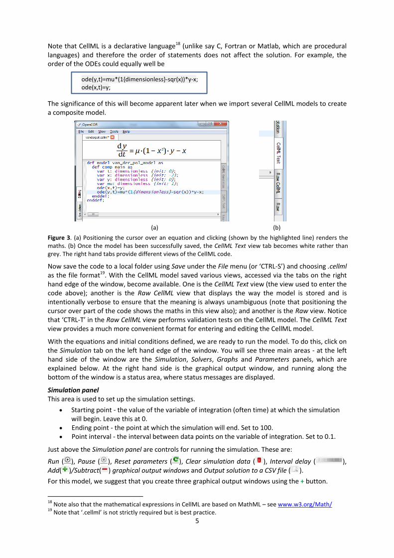
Note that CellML is a declarative language18

(unlike say C, Fortran or Matlab, which are procedural

languages) and therefore the order of statements does not affect the solution. For example, the

order of the ODEs could equally well be

The significance of this will become apparent later when we import several CellML models to create

a composite model.

(a) (b)

Figure 3. (a) Positioning the cursor over an equation and clicking (shown by the highlighted line) renders the

maths. (b) Once the model has been successfully saved, the CellML Text view tab becomes white rather than

grey. The right hand tabs provide different views of the CellML code.

Now save the code to a local folder using Save under the File menu (or ‘CTRL-S’) and choosing .cellml as the file format

19. With the CellML model saved various views, accessed via the tabs on the right

hand edge of the window, become available. One is the CellML Text view (the view used to enter the

code above); another is the Raw CellML view that displays the way the model is stored and is

intentionally verbose to ensure that the meaning is always unambiguous (note that positioning the

cursor over part of the code shows the maths in this view also); and another is the Raw view. Notice

that ‘CTRL-T’ in the Raw CellML view performs validation tests on the CellML model. The CellML Text view provides a much more convenient format for entering and editing the CellML model.

With the equations and initial conditions defined, we are ready to run the model. To do this, click on

the Simulation tab on the left hand edge of the window. You will see three main areas - at the left

hand side of the window are the Simulation, Solvers, Graphs and Parameters panels, which are

explained below. At the right hand side is the graphical output window, and running along the

bottom of the window is a status area, where status messages are displayed.

Simulation panel This area is used to set up the simulation settings.

x Starting point - the value of the variable of integration (often time) at which the simulation

will begin. Leave this at 0.

x Ending point - the point at which the simulation will end. Set to 100.

x Point interval - the interval between data points on the variable of integration. Set to 0.1.

Just above the Simulation panel are controls for running the simulation. These are:

Run ( ), Pause ( ), Reset parameters ( ), Clear simulation data ( ), Interval delay ( ),

Add( )/Subtract( ) graphical output windows and Output solution to a CSV file ( ).

For this model, we suggest that you create three graphical output windows using the + button.

18

Note also that the mathematical expressions in CellML are based on MathML – see www.w3.org/Math/ 19

Note that ‘.cellml’ is not strictly required but is best practice.

ode(y,t)=mu*(1{dimensionless}-sqr(x))*y-x;

ode(x,t)=y;

6

Solvers panel This area is used to configure the solver that will run the simulation.

x Name - this is used to set the solver algorithm. It will be set by default to be the most

appropriate solver for the equations you are solving. OpenCOR allows you to change this to

another solver appropriate to the type of equations you are solving if you choose to. For

example, CVODE for ODE (ordinary differential equation) problems, IDA for DAE (differential

algebraic equation) problems, KINSOL for NLA (non-linear algebraic) problems20

.

x Other parameters for the chosen solver – e.g. Maximum step, Maximum number of steps,

and Tolerance settings for CVODE and IDA. For more information on the solver parameters,

please refer to the documentation for the particular solver.

Note: these can all be left at their default values for our simple demo problem21

.

Graphs panel This shows what parameters are being plotted once these have been defined in the Parameters panel. These can be selected/deselected by clicking in the box next to a parameter.

Parameters panel This panel lists all the model parameters, and allows you to select one or more to plot against the

variable of integration or another parameter in the graphical output windows. OpenCOR supports

graphing of any parameter against any other. All variables from the model are listed here, arranged

by the components in which they appear, and in alphabetical order. Parameters are displayed with

their variable name, their value, and their units. The icons alongside them have the following

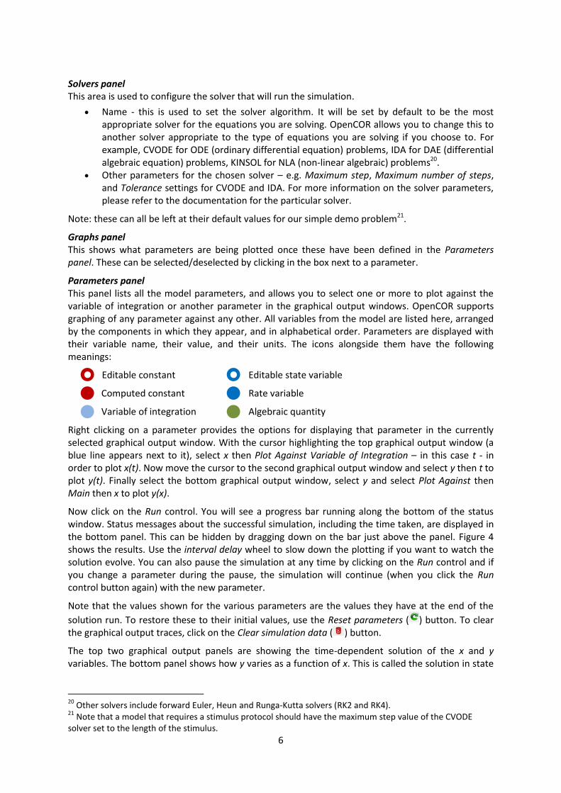
meanings:

Editable constant Editable state variable

Computed constant Rate variable

Variable of integration Algebraic quantity

Right clicking on a parameter provides the options for displaying that parameter in the currently

selected graphical output window. With the cursor highlighting the top graphical output window (a

blue line appears next to it), select x then Plot Against Variable of Integration – in this case t - in

order to plot x(t). Now move the cursor to the second graphical output window and select y then t to

plot y(t). Finally select the bottom graphical output window, select y and select Plot Against then

Main then x to plot y(x).

Now click on the Run control. You will see a progress bar running along the bottom of the status

window. Status messages about the successful simulation, including the time taken, are displayed in

the bottom panel. This can be hidden by dragging down on the bar just above the panel. Figure 4

shows the results. Use the interval delay wheel to slow down the plotting if you want to watch the

solution evolve. You can also pause the simulation at any time by clicking on the Run control and if

you change a parameter during the pause, the simulation will continue (when you click the Run

control button again) with the new parameter.

Note that the values shown for the various parameters are the values they have at the end of the

solution run. To restore these to their initial values, use the Reset parameters ( ) button. To clear

the graphical output traces, click on the Clear simulation data ( ) button.

The top two graphical output panels are showing the time-dependent solution of the x and y

variables. The bottom panel shows how y varies as a function of x. This is called the solution in state

20

Other solvers include forward Euler, Heun and Runga-Kutta solvers (RK2 and RK4). 21

Note that a model that requires a stimulus protocol should have the maximum step value of the CVODE

solver set to the length of the stimulus.

7

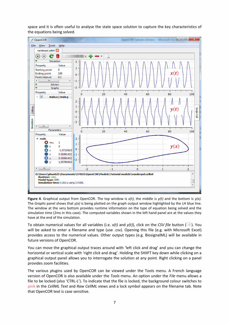
space and it is often useful to analyse the state space solution to capture the key characteristics of

the equations being solved.

Figure 4. Graphical output from OpenCOR. The top window is x(t), the middle is y(t) and the bottom is y(x). The Graphs panel shows that y(x) is being plotted on the graph output window highlighted by the LH blue line.

The window at the very bottom provides runtime information on the type of equation being solved and the

simulation time (2ms in this case). The computed variables shown in the left hand panel are at the values they

have at the end of the simulation.

To obtain numerical values for all variables (i.e. x(t) and y(t)), click on the CSV file button ( ). You

will be asked to enter a filename and type (use .csv). Opening this file (e.g. with Microsoft Excel)

provides access to the numerical values. Other output types (e.g. BiosignalML) will be available in

future versions of OpenCOR.

You can move the graphical output traces around with ‘left click and drag’ and you can change the horizontal or vertical scale with ‘right click and drag’. Holding the SHIIFT key down while clicking on a graphical output panel allows you to interrogate the solution at any point. Right clicking on a panel

provides zoom facilities.

The various plugins used by OpenCOR can be viewed under the Tools menu. A French language

version of OpenCOR is also available under the Tools menu. An option under the File menu allows a

file to be locked (also ‘CTRL-L’). To indicate that the file is locked, the background colour switches to

pink in the CellML Text and Raw CellML views and a lock symbol appears on the filename tab. Note

that OpenCOR text is case sensitive.

𝒙(𝒕)

𝒚(𝒕)

𝒚(𝒙)

8

4. Open an existing CellML file from a local directory or the Physiome Model Repository

Go to the File menu and select Open.... Browse to the folder that contains your existing models and

select one. Note that this brings up a new tabbed window and you can have any number of CellML

models open at the same time in order to quickly move between them. A model can be removed

from this list by clicking on next to the CellML model name.

You can also access models from the left hand panel in Figure 1(a). If this panel is not currently

visible, use ‘CTRL-spacebar’ to make it reappear. Models can then be accessed from any one of the three subdivisions of this panel – File Browser, Physiome Model Repository or File Organiser. For a

file under File Browser or File Organiser, either double-click it or ‘drag&drop’ it over the central

workspace to open that model. Clicking on a model in the Physiome Model Repository (PMR) (e.g.

Chen, Popel, 2007) opens a new browser window with that model (PMR is covered in more detail in

Section 13). You can either load this model directly into OpenCOR or create an identical copy (clone)

of the model in your local directory. Note that PMR contains workspaces and exposures. Workspaces

are online environments for the collaborative development of models (e.g. by geographically

dispersed groups) and can have password protected access. Exposures are workspaces that are

exposed for public view and mostly contain models from peer-reviewed journal publications. There

are about 600 exposures based on journal papers and covering many areas of cell processes and

other ODE/algebraic models, but these are currently being supplemented with reusable protein-

based models – see discussion in a Section 13.

To load a model directly into OpenCOR, click on the right-most of the two buttons in Figure 5 - this

lists the CellML models in that exposure - and then click on the model you want. Clicking on the left

hand button copies the PMR workspace to a local directory that you specify. This is useful if you

want to use that model as a template for a new one you are creating.

Figure 5. The Physiome Model Repository (PMR) window listing all

PMR models. These can be opened from within OpenCOR using

the two buttons to the right of a model, as explained below.

RH button lists all CellML files for this model. Clicking on

one of those uploads the model into OpenCOR.

LH button copies the PMR workspace to a local directory.

9

5. A simple first order ODE

The simplest example of a first order ODE is

with the solution

( ) . ( )

/ ,

where ( ) or , the value of ( ) at , is the initial condition. The final steady state solution as

is ( | )

(see Figure 6). Note that

is called the time constant of the

exponential decay, and that

( ) . ( )

/ .

At , ( ) has therefore fallen to (or about 37%) of the difference between the initial ( ( ))

and final steady state ( ( )) values.22

Choosing parameters and ( ) , the CellML Text for this model is

def model first_order_model as

def comp main as

var t: dimensionless {init: 0}; var y: dimensionless {init: 5}; var a: dimensionless {init: 1}; var b: dimensionless {init: 2};

ode(y,t)=-a*y+b;

enddef;

enddef;

The solution by OpenCOR is shown in Figure 7(a) for these parameters (a decaying exponential) and

in Figure 7(b) for parameters and ( ) (an inverted decaying exponential). Note

the simulation panel with Ending point=10, Point interval=0.1. Try putting .

(a) (b)

Figure 7. OpenCOR output ( ) for the simple ODE model with parameters (a) and ( ) ,

and (b) and ( ) . The red arrow indicates the point at which the trace reaches the time

constant ( or ≈37% of the difference between the initial and final solution values). The black arrows

indicate the initial and final (steady state) solutions. Note that the parameters on the left have been reset to

their initial values for this figure – normally they would be at their final solution values.

22 It is often convenient to write a first order equation as

, so that its solution is expressed in

terms of time constant , initial condition and steady state solution as: ( ) ( ) ⁄ .

𝝉 𝟏

𝝉 𝟏

𝒚

𝒚

𝒚𝟎

𝒚𝟎

exponential

decay

Figure 6. Solution of 1st

order equation.

𝑡

𝑦(𝑡)

𝑏𝑎

𝑦

𝑦

10

These two solutions have the same exponential time constant ( ) but different initial and

final (steady state) values.

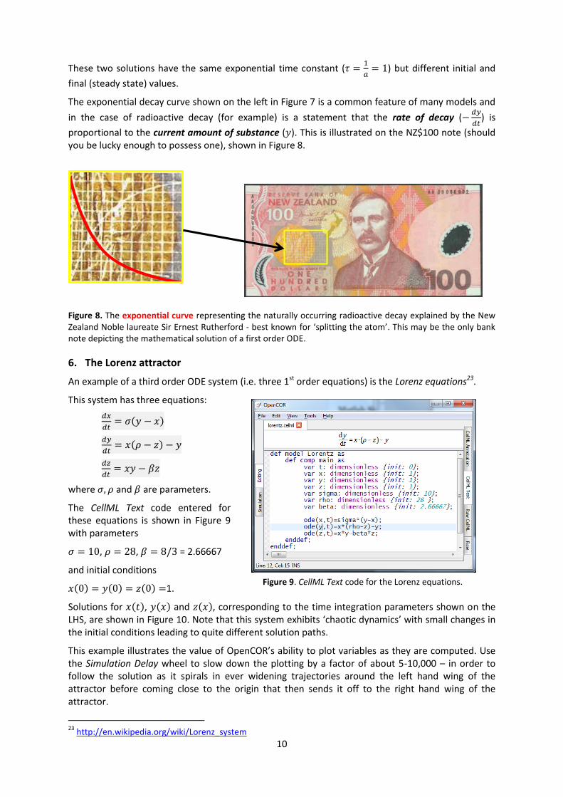
The exponential decay curve shown on the left in Figure 7 is a common feature of many models and

in the case of radioactive decay (for example) is a statement that the rate of decay (

) is

proportional to the current amount of substance ( ). This is illustrated on the NZ$100 note (should

you be lucky enough to possess one), shown in Figure 8.

Figure 8. The exponential curve representing the naturally occurring radioactive decay explained by the New

Zealand Noble laureate Sir Ernest Rutherford - best known for ‘splitting the atom’. This may be the only bank

note depicting the mathematical solution of a first order ODE.

6. The Lorenz attractor

An example of a third order ODE system (i.e. three 1st

order equations) is the Lorenz equations23.

This system has three equations:

( )

( )

where and are parameters.

The CellML Text code entered for

these equations is shown in Figure 9

with parameters

, , = 2.66667

and initial conditions

( ) ( ) ( ) 1.

Solutions for ( ), ( ) and ( ), corresponding to the time integration parameters shown on the

LHS, are shown in Figure 10. Note that this system exhibits ‘chaotic dynamics’ with small changes in

the initial conditions leading to quite different solution paths.

This example illustrates the value of OpenCOR’s ability to plot variables as they are computed. Use

the Simulation Delay wheel to slow down the plotting by a factor of about 5-10,000 – in order to

follow the solution as it spirals in ever widening trajectories around the left hand wing of the

attractor before coming close to the origin that then sends it off to the right hand wing of the

attractor.

23

http://en.wikipedia.org/wiki/Lorenz_system

Figure 9. CellML Text code for the Lorenz equations.

11

Figure 10. Solutions of the Lorenz equations. Note that the parameters on the left have been reset to their

initial values for this figure – normally they would be at their final solution values.

Solutions to the Lorenz equations are organised by the 2D ‘Lorenz manifold’. This surface has a very

beautiful shape and has become an art form – even rendered in crochet!24

(See Figure 11).

Exercise for the reader

Another example of intriguing and unpredictable behaviour from a simple deterministic ODE system

is the ‘blue sky catastrophe’ model [9] defined by the following equations:

with parameter and initial conditions ( ) , ( ) . Run to with

and plot ( ) and ( ). Also try with to see how sensitive the solution is to small

changes in parameter values. 24

www.math.auckland.ac.nz/~hinke/crochet/

𝒙(𝒕)

𝒚(𝒙)

𝒛(𝒙)

Figure 11. The crocheted Lorenz manifold

made by Hinke Osinga and Bernd Krauskopf

of the Mathematics Department at the

University of Auckland, New Zealand.

12

7. A model of ion channel gating and current: Introducing CellML units

A good example of a model based on a first order equation is the one used by Hodgkin and Huxley

[10] to describe the gating behaviour of an ion channel (see also next three sections). Before we

describe the gating behaviour of an ion channel, however, we need to explain the concepts of the

‘Nernst potential’ and channel conductance.

An ion channel is a protein or protein complex embedded in the bilipid membrane surrounding a cell

and containing a pore through which an ion (or ) can pass when the channel is open. If the

concentration of this ion is , - outside the cell and , - inside the cell, the force driving an ion

through the pore is calculated from the change in entropy.

Entropy (J.K-1

) is a measure of the number of microstates

available to a system, as defined by Boltzmann’s equation , where is the number of ways of arranging a given

distribution of microstates of a system and is Boltzmann’s constant

25. The driving force for ion movement is the dispersal of

energy into a more probable distribution (see Figure 12; cf the

second law of thermodynamics26

).

The energy change associated with this change of entropy

at temperature is (J).

For a given volume of fluid the number of microstates

available to a solute (and hence the entropy of the solute) at a

high concentration is less than that for a low concentration27

. The

energy difference driving ion movement from a high ion

concentration , - (lower entropy) to a lower ion concentration

, - (higher entropy) is therefore

. [ ] [ ] /

0 1

0 1 (J.ion

-1)

or

0 1

0 1

(J.mol

-1).

≈ 1.34x10-23

(J.K-1

) x 6.02x1023

(mol-1) ≈ 8.4 (J.mol

-1K

-1) is the ‘universal gas constant’28

.

At 25°C (298K), ≈ 2.5 kJ.mol-1

.

Every positively charged ion that crosses the membrane raises the

potential difference and produces an electrostatic driving force

that opposes the entropic force (see Figure 13). To move an

electron of charge e (≈1.6x10-19

C) through a voltage change of

(V) requires energy �(J) and therefore the energy needed

to move an ion �of valence z=1 (the number of charges per ion)

through a voltage change of is ��(J.ion-1

) or

(J.mol-1

). Using Faraday’s constant , where

≈0.96x105 C.mol

-1, the change in energy density at the macroscopic scale is (J.mol

-1).

25

The Brownian motion of individual molecules has energy (J), where the Boltzmann constant is

approximately 1.34x10-23

(J.K-1

). At 25°C, or 298K, = 4.10-21

(J) is the minimum amount of energy to contain

a ‘bit’ of information at that temperature. 26

The first law of thermodynamics states that energy is conserved, and the second law (that natural processes

are accompanied by an increase in entropy of the universe) deals with the distribution of energy in space. 27

At infinitely high concentration the specified volume is jammed packed with solute and the entropy is zero. 28

is Avogadro’s number (6.023x1023) and is the scaling factor between molecular and macroscopic

processes. Boltzmann’s constant and electron charge e operate at the atomic/molecular scale. Their effect

at the physiological scale is via the universal gas constant and Faraday’s constant .

Figure 12. Distribution of microstates

in a system [11]. The 16 particles in a

confined region (left) have only one

possible arrangement (𝑊 = 1) and

therefore zero entropy (𝑘𝐵𝑙𝑛𝑊 ).

When the barrier is removed and the

number of possible locations for each

particle increases 4x (right), the

number of possible arrangements for

the 16 particles increases by 416

and

the increase in entropy is therefore

ln(416

) or 16ln4. The thermal energy

(temperature) of the previously

confined particles on the left has

been redistributed in space to

achieve a more probable (higher

entropy) state. If we now added more

particles to the container on the right,

the concentration would increase and

the entropy would decrease.

Figure 13.The balance between

entropic and electrostatic forces

determines the Nernst potential.

𝑖 𝑌

,𝑌 -𝑖

,𝑌 -𝑜

Intracellular

Extracellular

13

(a) (b)

Figure 16. Transient behaviour for one

gate (left) and 𝛾 gates in series (right).

Note that the right hand graph has an

initial S-shaped increase, reflecting

the multiple gates in series.

1

𝑡

𝑦

𝑡

𝑦𝛾

0

No further movement of ions takes place when the force for entropy driven ion movement exactly

equals the opposing electrostatic driving force associated with charge movement:

0 1

0 1

(J.mol

-1) or

0 1

0 1

(J.C

-1 or V)

where is the ‘equilibrium’ or ‘Nernst’ potential for . At 25°C (298K),

(J.C-1) ≈ 25mV.

For an open channel the electrochemical current flow is

driven by the open channel conductance times the

difference between the transmembrane voltage and the

Nernst potential for that ion:

( ).

This defines a linear current-voltage relation (‘Ohms law’) as shown in Figure 14. The gates to be discussed below modify

this open channel conductance.

To describe the time dependent transition between the

closed and open states of the channel, Hodgkin and Huxley

introduced the idea of channel gates that control the

passage of ions through a membrane ion channel. If the

fraction of gates that are open is y, the fraction of gates

that are closed is 1-y, and a first order ODE can be used to

describe the transition between the two states (see Fig.15):

( )

where is the opening rate and is the closing rate.

The solution to this ODE is

( )

The constant can be interpreted as ( )

as

in the previous example and, with ( ) (i.e. all gates

initially shut), the solution looks like Figure 16(a).

The experimental data obtained by Hodgkin and Huxley for the squid axon, however, indicated that

the initial current flow began more slowly (Figure 16b) and they modelled this by assuming that the

ion channel had gates in series so that conduction would only occur when all gates were at least

partially open. Since is the probability of a gate being open, is the probability of all gates

being open (since they are assumed to be independent) and the current through the channel is

( )

where ( ) is the steady state current through the open gate.

We can represent this in OpenCOR with a simple extension of the first order ODE model, but in

developing this model we will also demonstrate the way in which CellML deals with units29

.

29

The decision to deal with units in CellML, rather than just ignoring them or insisting that all equations are

represented in dimensionless form, was made in order to be able to be able to check the physical consistency

of all terms in each equation. It is well accepted in engineering analysis that thinking about and dealing with

units is a key aspect of modelling. Taking the ratio of dimensionally consistent terms provides non-dimensional

numbers which can be used to decide when a term in an equation can be omitted in the interests of modelling

simplicity. We investigate this idea further in a later section.

𝛼𝑦

Figure 15. Ion channel gating kinetics.

𝑦 is the fraction of gates in the open

state. 𝛼𝑦 and 𝛽𝑦 are the rate

constants for opening and closing,

respectively.

𝛽𝑦 𝑦

𝑦

𝑖 𝑌

𝐸𝑌 𝑉

𝑖 𝑌 𝑔 𝑌(𝑉 𝐸𝑌)

Figure 14. Open channel linear current-

voltage relation.

14

There are seven base physical quantities defined by the Système International d’Unités (SI)30

.

These are (with their SI units):

x length (meter or m)

x time (second or s)

x amount of substance (mole)

x temperature (K)

x mass (kilogram or kg)

x current (amp or A)

x luminous intensity (candela).

All other units are derived from these seven. Additional derived units that CellML defines intrinsically

(with their dependence on previously defined units) are: Hz (s−1

); Newton, N (kg⋅m⋅s−2); Joule, J

(N.m); Pascal, Pa (N.m-2

); Watt, W (J.s−1

); Volt, V (W.A−1

); Siemen, S (A.V−1

); Ohm, (V.A−1

);

Coulomb, C (s.A); Farad, F (C.V−1

); Weber, Wb (V.s); and Henry, H (Wb.A−1

). Multiples and fractions

of these are defined as follows:

Multiples

Prefix deca hecto kilo mega giga tera peta exa zetta yotta

Symbol da h k M G T P E Z Y

Factor 100 10

1 10

2 10

3 10

6 10

9 10

12 10

15 10

18 10

21 10

24

Fractions

Prefix deci centi milli micro nano pico femto atto zepto yocto

Symbol d c m μ n p f a z y

Factor 100 10

−1 10

−2 10

−3 10

−6 10

−9 10

−12 10

−15 10

−18 10

−21 10

−24

Units for this model, with multiples and fractions, are illustrated in the following CellML Text code:

def model first_order_model as

def unit millisec as

unit second {pref: milli}; enddef; def unit per_millisec as

unit second {pref: milli, expo: -1}; enddef;

def unit millivolt as

unit volt {pref: milli}; enddef;

def unit microA_per_cm2 as

unit ampere {pref: micro}; unit metre {pref: centi, expo: -2}; enddef; def unit milliS_per_cm2 as

unit siemens {pref: milli}; unit metre {pref: centi, expo: -2}; enddef;

def comp ion_channel as

var V: millivolt {init: 0}; var t: millisec {init: 0}; var y: dimensionless {init: 0}; var E_y: millivolt {init: -85}; var i_y: microA_per_cm2;

var g_y: milliS_per_cm2 {init: 36}; var gamma: dimensionless {init: 4}; var alpha_y: per_millisec {init: 1}; var beta_y: per_millisec {init: 2};

ode(y, t) = alpha_y*(1{dimensionless}-y)-beta_y*y;

i_y = g_y*pow(y, gamma)*(V-E_y);

enddef; enddef;

30

http://en.wikipedia.org/wiki/International_System_of_Units

Define units and initial conditions for variables

Define units for time as millisecs

Define per_millisec units

Define units for voltage as millivolts

Define units for current as microAmps per cm2

Define units for conductance as milliSiemens per cm2

Define ODE for gating variable y

Define channel current

15

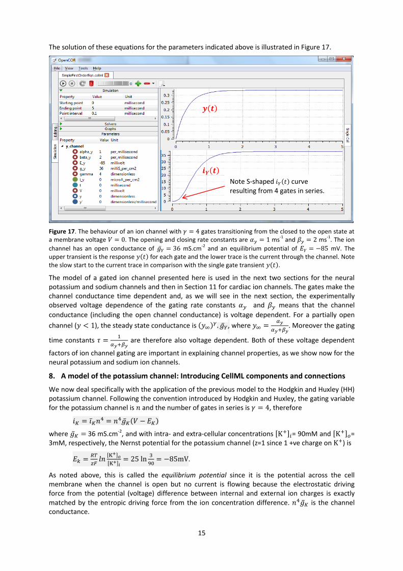
The solution of these equations for the parameters indicated above is illustrated in Figure 17.

Figure 17. The behaviour of an ion channel with gates transitioning from the closed to the open state at

a membrane voltage . The opening and closing rate constants are ms-1

and ms-1

. The ion

channel has an open conductance of mS.cm-2

and an equilibrium potential of mV. The

upper transient is the response ( ) for each gate and the lower trace is the current through the channel. Note

the slow start to the current trace in comparison with the single gate transient ( ).

The model of a gated ion channel presented here is used in the next two sections for the neural

potassium and sodium channels and then in Section 11 for cardiac ion channels. The gates make the

channel conductance time dependent and, as we will see in the next section, the experimentally

observed voltage dependence of the gating rate constants and means that the channel

conductance (including the open channel conductance) is voltage dependent. For a partially open

channel ( ), the steady state conductance is ( ) , where

. Moreover the gating

time constants

are therefore also voltage dependent. Both of these voltage dependent

factors of ion channel gating are important in explaining channel properties, as we show now for the

neural potassium and sodium ion channels.

8. A model of the potassium channel: Introducing CellML components and connections

We now deal specifically with the application of the previous model to the Hodgkin and Huxley (HH)

potassium channel. Following the convention introduced by Hodgkin and Huxley, the gating variable

for the potassium channel is and the number of gates in series is , therefore

( )

where 36 mS.cm-2

, and with intra- and extra-cellular concentrations , - = 90mM and , - =

3mM, respectively, the Nernst potential for the potassium channel (z=1 since 1 +ve charge on ) is

,

- , -

.

As noted above, this is called the equilibrium potential since it is the potential across the cell

membrane when the channel is open but no current is flowing because the electrostatic driving

force from the potential (voltage) difference between internal and external ion charges is exactly

matched by the entropic driving force from the ion concentration difference. is the channel

conductance.

Note S-shaped 𝑖𝑌(𝑡) curve

resulting from 4 gates in series.

𝒚(𝒕)

𝒊𝒀(𝒕)

16

The gating kinetics are described (as before) by

( )

with time constant

(see page 9).

The main difference from the gating model in our previous

example is that Hodgkin and Huxley found it necessary to make

the rate constants functions of the membrane potential (see

Figure 18) as follows31

:

( )

( )

;

( ) .

Note that under steady state conditions when and

, |

.

The voltage dependence of the steady state channel

conductance is then

.

/ .

(see Figure 18). The steady state current-voltage relation for

the channel is illustrated in Figure 19.

These equations are captured with OpenCOR CellML Text view (together with the previous unit

definitions) on the next page. But first we need to explain some further CellML concepts.

We introduced CellML units above. We now need to

introduce three more CellML constructs: components,

connections (mappings between components) and groups.

For completeness we also show one other construct in

Figure 20 that will be used later in Section 10: imports.

Defining components serves two purposes: it preserves a

modular structure for CellML models, and allows these

component modules to be imported into other models, as

we will illustrate later [2]. For the potassium channel

model we define components representing (i) the

environment, (ii) the potassium channel conductivity, and

(iii) the dynamics of the n-gate.

Since certain variables (t, V and n) are shared between

components, we need to also define the component maps

as indicated in the CellML Text view on the next page.

31 The original expression in the HH paper used

( )

( )

and , where is defined

relative to the resting potential (-75mV) with +ve corresponding to +ve inward current and ( ).

CellML model

component variable

math

group relationshipRef

componentRef

imported units

imported component

import

units unit

connection mapComponent

mapVariable

Figure 20. Key entities in a CellML model.

1

𝛼𝑛

𝛽𝑛

𝑉

Figure 18. Voltage dependence of

rate constants 𝛼𝑛 and 𝛽𝑛 (ms-1

),

time constant 𝜏𝑛(ms) and relative

conductance 𝑔𝑆𝑆 𝑔 𝑌 .

𝜏𝑛

𝑔𝑆𝑆 𝑔 𝑌

𝑉

Figure 19. The steady-state current-

voltage relation for the potassium

channel.

𝐸𝐾

𝐼

Needs checking

17

The CellML Text code for the potassium ion channel model is as follows32

:

Potassium_ion_channel.cellml

def model potassium_ion_channel as

def unit millisec as

unit second {pref: milli}; enddef; def unit per_millisec as

unit second {pref: milli, expo: -1}; enddef; def unit millivolt as

unit volt {pref: milli}; enddef;

def unit per_millivolt as

unit millivolt {expo: -1};

enddef;

def unit per_millivolt_millisec as

unit per_millivolt;

unit per_millisec;

enddef; def unit microA_per_cm2 as

unit ampere {pref: micro}; unit metre {pref: centi, expo: -2}; enddef;

def unit milliS_per_cm2 as

unit siemens {pref: milli}; unit metre {pref: centi, expo: -2}; enddef; def unit mM as

unit mole {pref: milli}; enddef;

def comp environment as

var V: millivolt { pub: out}; var t: millisec {pub: out}; V = sel

case (t > 5 {millisec}) and (t < 15 {millisec}): -85.0 {millivolt}; otherwise:

0.0 {millivolt}; endsel;

enddef;

def group as encapsulation for

comp potassium_channel incl

comp potassium_channel_n_gate;

endcomp;

enddef;

def comp potassium_channel as

var V: millivolt {pub: in , priv: out}; var t: millisec {pub: in, priv: out}; var n: dimensionless {priv: in}; var i_K: microA_per_cm2 {pub: out}; var g_K: milliS_per_cm2 {init: 36}; var Ko: mM {init: 3}; var Ki: mM {init: 90}; var RTF: millivolt {init: 25}; var E_K: millivolt; var K_conductance: milliS_per_cm2 {pub: out};

E_K=RTF*ln(Ko/Ki);

K_conductance = g_K*pow(n, 4{dimensionless});

i_K = K_conductance*(V-E_K);

enddef;

32

From here on we use a coloured background to identify code blocks that relate to a particular CellML

construct: units, components, mappings and encapsulation groups and later imports.

Define voltage step

Define units

Define component ‘environment’

Define component ‘potassium channel’

Define encapsulation of n_gate

18

def comp potassium_channel_n_gate as

var V: millivolt {pub: in}; var t: millisec {pub: in}; var n: dimensionless {init: 0.325, pub: out}; var alpha_n: per_millisec;

var beta_n: per_millisec;

alpha_n = 0.01{per_millivolt_millisec}*(V+10{millivolt})

/(exp((V+10{millivolt})/10{millivolt})-1{dimensionless});

beta_n = 0.125{per_millisec}*exp(V/80{millivolt});

ode(n, t) = alpha_n*(1{dimensionless}-n)-beta_n*n;

enddef;

def map between environment and potassium_channel for

vars V and V;

vars t and t;

enddef; def map between potassium_channel and potassium_channel_n_gate for

vars V and V;

vars t and t;

vars n and n;

enddef;

enddef;

Note that several other features have been added:

¾ the event control select case which indicates that the voltage is specified to jump from 0mV

to -85mV at t=5ms then back to 0mV at t=15ms. This is only used here in order to test the K

channel model; when the potassium_channel component is later imported into a neuron

model, the environment component is not imported.

¾ the use of encapsulation to embed the potassium_channel_n_gate inside the

potassium_channel. This avoids the need to establish mappings from environment to

potassium_channel_n_gate since the gate component is entirely within the channel

component.

¾ the use of * + and * + to indicate which variables are either supplied as inputs to

a component or produced as outputs from a component33

. Any variables not labelled as in or

out are local variables or parameters defined and used only within that component. Public

(and private) interfaces are discussed in more detail in the next section.

We now use OpenCOR, with Ending point 40 and Point interval 0.1, to solve the equations for the

potassium channel under a voltage step condition in which the membrane voltage is clamped

initially at 0mV and then stepped down to -85mV for 10ms before being returned to 0mV. At 0mV,

the steady state value of the n gate is

0.324 and, at -85mV, 0.945.

The voltage traces are shown at the top of Figure 21. The n-gate response, shown next, is to open

further from its partially open value of 0.324 at 0mV and then plateau at an almost fully open

state of 0.945 at the Nernst potential -85mV before closing again as the voltage is stepped back

to 0mV. Note that the gate opening behaviour (set by the voltage dependence of the opening

rate constant) is faster than the closing behaviour (set by the voltage dependence of the closing

rate constant). The channel conductance ( ) is shown next – note the initial s-shaped

conductance increase caused by the (four gates in series) effect on conductance. Finally the

channel current conductance x ( ) is shown at the bottom. Because the voltage is

clamped at the Nernst potential (-85mV) during the period when the gate is opening, there is no

current flow, but when the voltage is stepped back to 0mV, the open gates begin to close and the

33

Note that a later version of CellML will remove the terms in and out since it is now thought that the direction

of information flow should not be constrained.

Define mappings between components for

variables that are shared between these

components

Define component ‘potassium channel n gate’

19

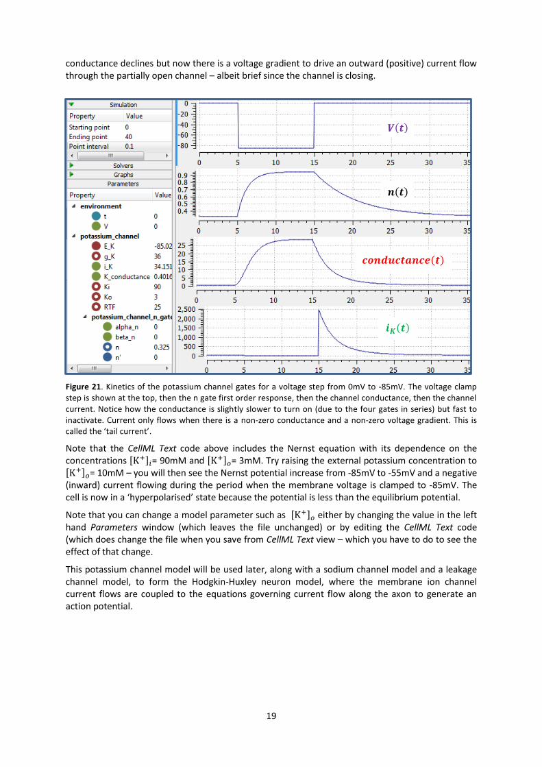
conductance declines but now there is a voltage gradient to drive an outward (positive) current flow

through the partially open channel – albeit brief since the channel is closing.

Figure 21. Kinetics of the potassium channel gates for a voltage step from 0mV to -85mV. The voltage clamp

step is shown at the top, then the n gate first order response, then the channel conductance, then the channel

current. Notice how the conductance is slightly slower to turn on (due to the four gates in series) but fast to

inactivate. Current only flows when there is a non-zero conductance and a non-zero voltage gradient. This is

called the ‘tail current’.

Note that the CellML Text code above includes the Nernst equation with its dependence on the

concentrations , - = 90mM and , - = 3mM. Try raising the external potassium concentration to

, - = 10mM – you will then see the Nernst potential increase from -85mV to -55mV and a negative

(inward) current flowing during the period when the membrane voltage is clamped to -85mV. The

cell is now in a ‘hyperpolarised’ state because the potential is less than the equilibrium potential.

Note that you can change a model parameter such as , - either by changing the value in the left

hand Parameters window (which leaves the file unchanged) or by editing the CellML Text code

(which does change the file when you save from CellML Text view – which you have to do to see the

effect of that change.

This potassium channel model will be used later, along with a sodium channel model and a leakage

channel model, to form the Hodgkin-Huxley neuron model, where the membrane ion channel

current flows are coupled to the equations governing current flow along the axon to generate an

action potential.

𝑽(𝒕)

𝒏(𝒕)

𝒄𝒐𝒏𝒅𝒖𝒄𝒕𝒂𝒏𝒄𝒆(𝒕)

𝒊𝑲(𝒕)

20

9. A model of the sodium channel: Introducing CellML encapsulation and interfaces

The HH sodium channel has two types of gate, an gate (of which there are 3) that is initially closed

( ) before activating and inactivating back to the closed state, and an gate that is initially open

( ) before activating and inactivating back to the open state. The short period when both types

of gate are open allows a brief window current to pass through the channel. Therefore,

( )

where 120 mS.cm-2

, and with , - = 30mM and , - = 140mM, the Nernst potential for

the sodium channel (z=1) is

,

- , -

.

The gating kinetics are described by

( ) ;

( )

where the voltage dependence of these four rate constants is determined experimentally to be34

( )

( )

;

( ) ;

( ) ;

( )

.

Before we construct a CellML model of the sodium channel, we first introduce some further CellML

concepts that help deal with the complexity of biological models: first the use of encapsulation groups and public and private interfaces to control the visibility of information in modular CellML

components. To understand encapsulation, it is useful to use the terms ‘parent’, ‘child’ and ‘sibling’.

We define the CellML components sodium_channel_m_gate

and sodium_channel_h_gate below. Each of these components

has its own equations (voltage-dependent gates and first

order gate kinetics) but they are both parts of one protein –

the sodium channel – and it is useful to group them into one

sodium_channel component as shown on the right:

We can then talk about the sodium channel as the parent of two children: the m gate and the h gate, which are therefore siblings. A private interface allows a parent to talk to its children and a public interface allows siblings to talk among themselves and to their parents (see Figure 22).

Figure 22. Children talk to each other as siblings, and to their parents, via public interfaces. But the outside

world can only talk to children through their parents via a private interface. Note that the siblings m_gate and

h_gate could talk via a public interface but only if a mapping is established between them (not needed here).

34 The HH paper used

( )

( )

; ;

;

( )

(see footnote on page 16).

def group as encapsulation for

comp sodium_channel incl

comp sodium_channel_m_gate;

comp sodium_channel_h_gate;

endcomp;

enddef;

Sib

lin

gs c

om

mu

nic

ate

via

pub

lic in

terf

ace

Parents communicate with children

via private to public interface

sodium_channel

m_gate

h_gate

m: {priv: in} & {pub: out}

h: {priv: in} & {pub: out}

V, t: {priv: out} & {pub: in}

environment

V, t:

{pub: out} {pub: in}

i_Na:

{pub: in} {pub: out}

Sib

lin

gs c

om

mu

nic

ate

via

pub

lic in

terf

ace

(bu

t n

ot

use

d h

ere

)

21

The OpenCOR CellML Text for the HH sodium ion channel is given below.

Sodium_ion_channel.cellml

def model sodium_ion_channel as def unit millisec as

unit second {pref: milli}; enddef; def unit per_millisec as

unit second {pref: milli, expo: -1}; enddef; def unit millivolt as

unit volt {pref: milli}; enddef; def unit per_millivolt as

unit millivolt {expo: -1};

enddef; def unit per_millivolt_millisec as

unit per_millivolt;

unit per_millisec;

enddef; def unit microA_per_cm2 as

unit ampere {pref: micro}; unit metre {pref: centi, expo: -2}; enddef; def unit milliS_per_cm2 as

unit siemens {pref: milli}; unit metre {pref: centi, expo: -2}; enddef; def unit mM as

unit mole {pref: milli}; enddef;

def comp environment as

var V: millivolt {pub: out}; var t: millisec {pub: out}; V = sel

case (t > 5 {millisec}) and (t < 15 {millisec}): -20.0 {millivolt}; otherwise:

-85.0 {millivolt}; endsel;

enddef;

def group as encapsulation for

comp sodium_channel incl

comp sodium_channel_m_gate;

comp sodium_channel_h_gate;

endcomp;

enddef;

def comp sodium_channel as

var V: millivolt {pub: in, priv: out}; var t: millisec {pub: in, priv: out }; var m: dimensionless {priv: in}; var h: dimensionless {priv: in}; var g_Na: milliS_per_cm2 {init: 120}; var E_Na: millivolt {init: 35}; var i_Na: microA_per_cm2 {pub: out}; var Nao: mM {init: 140}; var Nai: mM {init: 30}; var RTF: millivolt {init: 25}; var E_Na: millivolt; var Na_conductance: milliS_per_cm2 {pub: out};

E_Na=RTF*ln(Nao/Nai);

Na_conductance = g_Na*pow(m, 3{dimensionless})*h);

i_Na= Na_conductance*(V-E_Na);

enddef;

Define voltage step

Define units

Define component ‘environment’

Define component ‘sodium channel’

Define encapsulation of m_gate and h_gate

22

def comp sodium_channel_m_gate a s

var V: millivolt {pub: in}; var t: millisec {pub: in}; var alpha_m: per_millisec;

var beta_m: per_millisec;

var m: dimensionless {init: 0.05, pub: out};

alpha_m = 0.1{per_millivolt_millisec}*(V+25{millivolt})

/(exp((V+25{millivolt})/10{millivolt})-1{dimensionless});

beta_m = 4{per_millisec}*exp(V/18{millivolt});

ode(m, t) = alpha_m*(1{dimensionless}-m)-beta_m*m;

enddef;

def comp sodium_channel_h_gate as

var V: millivolt {pub: in}; var t: millisec {pub: in}; var alpha_h: per_millisec; var beta_h: per_millisec;

var h: dimensionless {init: 0.6, pub: out};

alpha_h = 0.07{per_millisec}*exp(V/20{millivolt});

beta_h = 1{per_millisec}/(exp((V+30{millivolt})/10{millivolt})+1{dimensionless});

ode(h, t) = alpha_h*(1{dimensionless}-h)-beta_h*h;

enddef;

def map between environment and sodium_channel for

vars V and V;

vars t and t;

enddef; def map between sodium_channel and sodium_channel_m_gate for

vars V and V;

vars t and t;

vars m and m;

enddef; def map between sodium_channel and sodium_channel_h_gate for

vars V and V;

vars t and t;

vars h and h;

enddef;

enddef;

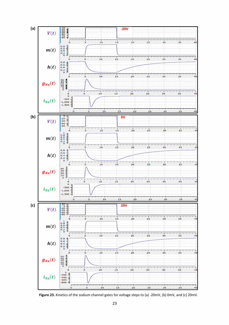
The results of the OpenCOR computation, with Ending point 40 and Point interval 0.1, are shown in

Figure 23 with plots of ( ), ( ), ( ), ( ) and ( ) for voltage steps from (a) -85mV to

-20mV, (b) -85mV to 0mV and (c) -85mV to 20mV. There are several things to note:

(i) The kinetics of the m-gate are much faster than the h-gate.

(ii) The opening behaviour is faster as the voltage is stepped to higher values since

reduces with increasing V (see Figure 18).

(iii) The sodium channel conductance rises (activates) and then falls (inactivates) under a positive

voltage step from rest since the three m-gates turn on but the h-gate turns off and the

conductance is a product of these. Compare this with the potassium channel conductance

shown in Figure 21 which is only reduced back to zero by stepping the voltage back to its

resting value – i.e. deactivating it.

(iv) The only time current flows through the sodium channel is during the brief period when

the m-gate is rapidly opening and the much slower h-gate is beginning to close. A small

current flows during the reverse voltage step but this is at a time when the h-gate is now

firmly off so the magnitude is very small.

(v) The large sodium current is an inward current and hence negative.

Note that the bottom trace does not quite line up at t=0 because the values shown on the axes are

computed automatically and hence can take more or less space depending on their magnitude.

Define mappings between

components for variables that are

shared between these components

Define component ‘sodium channel h gate’

Define component ‘sodium channel m gate’

23

Figure 23. Kinetics of the sodium channel gates for voltage steps to (a) -20mV, (b) 0mV, and (c) 20mV.

(a)

(b)

(c)

𝑽(𝒕)

𝒎(𝒕)

𝒉(𝒕)

𝒊𝑵𝒂(𝒕)

𝒈𝑵𝒂(𝒕)

𝑽(𝒕)

𝒎(𝒕)

𝒉(𝒕)

𝒊𝑵𝒂(𝒕)

𝒈𝑵𝒂(𝒕)

𝑽(𝒕)

𝒎(𝒕)

𝒉(𝒕)

𝒊𝑵𝒂(𝒕)

𝒈𝑵𝒂(𝒕)

-20V

0V

20V

24

10. A model of the nerve action potential: Introducing CellML imports

Here we describe the first (and most famous) model of nerve fibre electrophysiology based on the

membrane ion channels that we have discussed in the last two sections. This is the work by Alan

Hodgkin and Andrew Huxley in 1952 [10] that won them (together with John Eccles) the 1963 Noble

prize in Physiology or Medicine for "their discoveries concerning the ionic mechanisms involved in excitation and inhibition in the peripheral and central portions of the nerve cell membrane".

Cable equation

The cable equation was developed in 189035

to predict the degradation of an electrical signal passing

along the transatlantic cable. It is derived as follows:

If the voltage is raised at the left hand end of the cable (shown

by the deep red in Figure 24), a current (A) will flow that

depends on the voltage gradient, given by

(V.m-1

) and the

resistance (:.m-1), Ohm’s law gives

. But if the

cable leaks current (A.m-1

) per unit length of cable, conservation of current gives and

therefore, substituting for , .

/ . There are two sources of membrane current ,

one associated with the capacitance ( ) of the membrane,

, and one associated

with holes or channels in the membrane, . Inserting these into the RHS gives

.

/

Rearranging gives the cable equation (for constant ):

where all terms represent current density (current per membrane area) and have units of .

Action potentials The cable equation can be used to model the propagation of an

action potential along a neuron or any other excitable cell. The

‘leak’ current is associated primarily with the inward movement of sodium ions through the membrane ‘sodium channel’, giving

the inward membrane current , and the outward movement

of potassium ions through a membrane ‘potassium channel’, giving the outward current (see Figure 25). A further small leak current ( ) associated with chloride and other ions is also included.

When the membrane potential rises

due to axial current flow, the Na

channels open and the K channels close,

such that the membrane potential

moves towards the Nernst potential for

sodium. The subsequent decline of the

Na channel conductance and the

increasing K channel conductance as

the voltage drops rapidly repolarises

the membrane to its resting potential of

-85mV (see Figure 26).

35

http://en.wikipedia.org/wiki/Cable_theory

Figure 24. Current flow in a leaky cable.

equation.

𝑖𝑚

𝑖𝑎 𝑉 𝑥

I(V) during upstroke

of action potential

(depolarisation )

field 𝐶(𝒙)

I(V) during repolarisation

I

V 30mV -85mV

Figure 26. Current-voltage trajectory during an action potential.

Injection of outward current pulse

pushes V to a threshold where Na channels

open to allow a large inward (-ve) current

I(V) for open K channel

I(V) for open Na channel

Figure 25. Current flow in a neuron.

𝑖𝐾 𝑖𝑁𝑎 𝑖𝐾

𝑉

25

We can neglect36

the term (

) (the rate of change of axial current along the cable) for the

present models since we assume the whole cell is clamped with an axially uniform potential. We can

therefore obtain the membrane potential by integrating the first order ODE

( ) .

Figure 27. A schematic cell diagram describing the current flows across the

cell bilipid membrane that are captured in the Hodgkin-Huxley model. The

membrane ion channels are a sodium (Na+) channel, a potassium (K

+)

channel, and a leakage (L) channel (for chloride and other ions) through

which the currents INa, IK and IL flow, respectively.

We use this example to demonstrate the importing feature of CellML. CellML imports are used to

bring a previously defined CellML model of a component into the new model (in this case the Na and

K channel components defined in the previous two sections, together with a leakage ion channel

model specified below). Note that importing a component brings the children components with it

along with their connections and units, but it does not bring the siblings of that component with it.

To establish a CellML model of the HH equations we first lay out the model components with their

public and private interfaces (Figure 28).

Figure 28. Overall structure of the HH CellML model showing the encapsulation hierarchy (purple), the CellML

model imports (blue) and the other key parts (units, components & mappings) of the top level CellML model.

The HH model is the top level model. The CellML Text code for the HH model, together with the

leakage_channel model, is given on the next page. The imported potassium_ion_channel model and

sodium_ion_channel model are unchanged from the previous sections

36

This term is needed when determining the propagation of the action potential, including its wave speed.

Environment

Units

Imports

Groups

Mappings V, t: {pub: out} {pub: in}

Membrane

Sodium

channel

h_gate

m_gate

m: {priv: in} & {pub: out}

h: {priv: in} & {pub: out}

V, t: {priv: out} & {pub: in} Na

channel Import

Potassium

channel n_gate

n: {priv: in} & {pub: out}

V, t: {priv: out} & {pub: in}

K

channel Import

Leakage

channel

L

channel Import

Enca

psul

ate

sodium_ion_channel.cellml

potassium_ion_channel.cellml

leakage_ion_channel.cellml

HH.cellml

26

HH.cellml def model HH as def import using "sodium_ion_channel.cellml" for

comp Na_channel using comp sodium_channel;

enddef; def import using "potassium_ion_channel.cellml" for

comp K_channel using comp potassium_channel;

enddef; def import using "leakage_ion_channel.cellml" for

comp L_channel using comp leakage_channel;

enddef;

def unit millisec as

unit second {pref: milli};

enddef; def unit millivolt as

unit volt {pref: milli};

enddef; def unit microA_per_cm2 as

unit ampere {pref: micro};

unit metre {pref: centi, expo: -2};

enddef; def unit microF_per_cm2 as

unit farad {pref: micro};

unit metre {pref: centi, expo: -2};

enddef;

def group as encapsulation for

comp membrane incl

comp Na_channel; comp K_channel; comp L_channel; endcomp;

enddef;

def comp environment as

var V: millivolt {init: -85, pub: out};

var t: millisec {pub: out};

enddef;

def map between environment and membrane for

vars V and V;

vars t and t;

enddef; def map between membrane and Na_channel for

vars V and V;

vars t and t;

vars i_Na and i_Na;

enddef; def map between membrane and K_channel for

vars V and V;

vars t and t;

vars i_K and i_K;

enddef; def map between membrane and L_channel for

vars V and V;

vars i_L and i_L;

enddef;

def comp membrane as

var V: millivolt {pub: in, priv: out};

var t: millisec {pub: in, priv: out};

var i_Na: microA_per_cm2 {pub: out, priv: in};

var i_K: microA_per_cm2 {pub: out, priv: in};

var i_L: microA_per_cm2 {pub: out, priv: in};

var Cm: microF_per_cm2 {init: 1};

var i_Stim: microA_per_cm2;

var i_Tot: microA_per_cm2;

i_Stim = sel

case (t >= 1{millisec}) and (t <= 1.2{millisec}):

100{microA_per_cm2};

otherwise:

0{microA_per_cm2};

endsel;

i_Tot = i_Stim + i_Na + i_K + i_L;

ode(V,t) = -i_Tot/Cm;

enddef;

enddef;

Leakage_ion_channel.cellml def model leakage_ion_channel as def unit millisec as

unit second {pref: milli};

enddef; def unit millivolt as

unit volt {pref: milli};

enddef; def unit per_millivolt as

unit millivolt {expo: -1};

enddef; def unit microA_per_cm2 as

unit ampere {pref: micro};

unit metre {pref: centi, expo: -2};

enddef; def unit milliS_per_cm2 as

unit siemens {pref: milli};

unit metre {pref: centi, expo: -2};

enddef;

def comp environment as

var V: millivolt {init: 0, pub: out};

var t: millisec {pub: out};

enddef;

def map between leakage_channel and environment for

vars V and V;

enddef;

def comp leakage_channel as

var V: millivolt {pub: in};

var i_L: microA_per_cm2 {pub: out};

var g_L: milliS_per_cm2 {init: 0.3};

var E_L: millivolt {init: -54.4};

i_L = g_L*(V-E_L);

enddef;

enddef;

Note that the CellML Text code for the

potassium and sodium channel modules

imported here is given on pages 17 and 21,

respectively.

27

Note that the only units that need to be defined for this top level HH model are the ones explicitly

required for the membrane component. All the other units, required for the various imported sub-

models, are imported along with the imported components.

The results generated by the HH model are shown in Figure 29.

Figure 29. Results from OpenCOR for the Hodgkin Huxley (HH) CellML model. The top panel shows the

generated action potential. Note that the stimulus current is not really needed as the background outward

leakage current is enough to drive the membrane potential up to the threshold for sodium channel opening.

𝒊𝑵𝒂(𝒕) 𝒊𝑲(𝒕) 𝒊𝑳 𝒊𝒔𝒕𝒊𝒎

𝑽(𝒕)

𝒊𝑵𝒂(𝒕)

𝒊𝑲(𝒕)

𝒊𝒔𝒕𝒊𝒎(𝒕)

28

Important note

It is often convenient to have the sub-models – in this case the sodium_ion_channel.cellml model,

the potassium_ion_channel.cellml model and the leakage_ion_channel.cellml model - loaded into

OpenCOR at the same time as the high level model (HH.cellml), as shown in Figure 30. If you make

changes to a model in the CellML Text view, you must save the file (CTRL-S) before running a new

simulation since the simulator works with the saved model. Furthermore, a change to a sub-model

will only affect the high level model which imports it if you also save the high level model (or use the

Reload option under the File menu). An asterisk appears next to the name of a file when a change

has been made and the file has not been saved. The asterisk disappears when the file is saved.

Figure 30. The HH.cellml model and its three sub-models are available under separate tabs in OpenCOR.

11. A model of the cardiac action potential: Importing units and parameters

We now examine the Noble 1962 model [12] that applied the Hodgkin-Huxley approach to cardiac

cells and thereby initiated the development of a long line of cardiac cell models that, in their human

cell formulation, are now used clinically and are the most sophisticated models of any cell type. It

was the incorporation of these models into whole heart bioengineering models that initiated the

Physiome Project. We also illustrate the use of imported units and imported parameter sets.

Cardiac cells have similar gradients of potassium and sodium ions that operate in a similar way to

neurons (as do all electrically active cells). There is one major difference, however, in the potassium

channel that holds the cells in their resting state at -85mV (HH neuron) or -100mV (cardiac Purkinje

cells). This difference is illustrated in Figure 31a. When the membrane potential is raised above the

equilibrium potential for potassium, the cardiac channel conductance shown by the dashed line

drops to nearly zero – i.e. it is an inward rectifier since it rectifies (‘cuts off’) the outward current that

otherwise would have flowed through the channel at that potential. This is an evolutionary

adaptation of the potassium channel to avoid loss of potassium ions out of the cell during the long

plateau phase of the cardiac action potential (Figure 31b) needed to give the heart time to contract.

This evolutionary change saves the additional energy that would otherwise be needed to pump

potassium ions back into the cell, but this Faustian “pact with the devil” is also the reason the heart is so susceptible to conduction failure (more on this later). To explain his data on Purkinje cells Noble

[12] postulated the existence of two inward rectifier potassium channels, one with a conductance

that showed voltage dependence but no significant time dependence and another with

conductance that showed less severe rectification with time dependent gating similar to the HH

four-gated potassium channel.

(a) (b)

Figure 31. Current-voltage relations (a) around the equilibrium potentials for the potassium and sodium

channels in cardiac cells. The sodium channel is similar to the one in neurons but the two potassium channels

have an inward rectifying property that stops leakage of potassium ions out of the cell when the membrane

potential (illustrated in (b)) is high during the plateau phase of the cardiac action potential.

I

V 30mV -100mV

I(V) for open K channels

Rectification

V

-100mV

30mV

t

Plateau

𝒊𝑲𝟏

𝒊𝑲𝟐

29

To model the cardiac action potential in Purkinje fibres (a cardiac cell specialised for rapid

conduction from the atrio-ventricular node to the apical ventricular myocardial tissue), Noble [12]

proposed two potassium channels (one of these being the inwardly rectifying potassium channel

described above and the other called the delayed potassium channel), one sodium channel (very

similar to the HH neuronal sodium channel) and one leakage channel (also similar to the HH one).

The equations for these are as follows: (as for the HH model, time is in ms, voltages are in mV,

concentrations are in mM, conductances are in mS, currents are in PA and capacitance is in PF).

Inward rectifying potassium channel (voltage dependent only)

( ), with ,

- , -

.

( )

( )

Inward rectifying potassium channel (voltage and time dependent)37

( ).

( ) , where

( )

( )

and

( ) .

Note that the rate constants here reflect a much slower onset of the time dependent change in

conductance than in the HH potassium channel.

Sodium channel

( )( ), with ,

- , -

.

where

( ) , where

( )

( )

and

( )

( )

( ) , where

( ) and

( )

Leakage channel

( ), with and .

Membrane equation

( ) where .

38

Figure 32 shows the structure of the model, including separate files for units, parameters, and the

three ion channels (the two potassium channels are lumped together). We include the Nernst

equations dependence on potassium and sodium ion concentrations in order to demonstrate the

use of parameter values, defined in a separate parameters file, that are read in at the top (whole cell

model) level and passed down to the individual ion channel models.

37

The second inwardly rectifying channel model was later replaced with two currents and , so that

modern cardiac cell models do not include but they do include the inward rectifier (see later section). 38

The Purkinje fibre membrane capacitance is 12 times higher than that found for squid axon. The use of

PF ensures unit consistency with ms, mV and PA since F is equivalent to C.V-1

or s.A.V-1

and therefore PA/PF or

PA/(ms.PA. mV-1

) on the RHS matches mV/ms on the LHS).

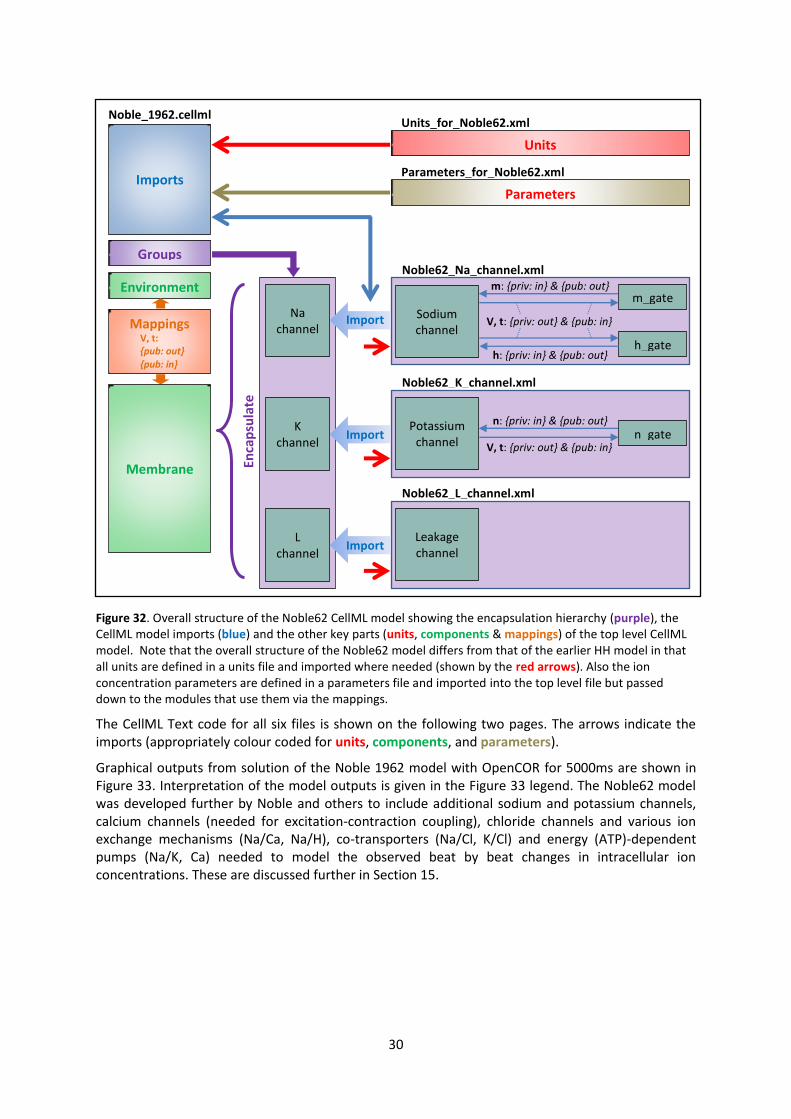
30

Figure 32. Overall structure of the Noble62 CellML model showing the encapsulation hierarchy (purple), the

CellML model imports (blue) and the other key parts (units, components & mappings) of the top level CellML

model. Note that the overall structure of the Noble62 model differs from that of the earlier HH model in that

all units are defined in a units file and imported where needed (shown by the red arrows). Also the ion

concentration parameters are defined in a parameters file and imported into the top level file but passed

down to the modules that use them via the mappings.

The CellML Text code for all six files is shown on the following two pages. The arrows indicate the

imports (appropriately colour coded for units, components, and parameters).

Graphical outputs from solution of the Noble 1962 model with OpenCOR for 5000ms are shown in

Figure 33. Interpretation of the model outputs is given in the Figure 33 legend. The Noble62 model

was developed further by Noble and others to include additional sodium and potassium channels,

calcium channels (needed for excitation-contraction coupling), chloride channels and various ion

exchange mechanisms (Na/Ca, Na/H), co-transporters (Na/Cl, K/Cl) and energy (ATP)-dependent

pumps (Na/K, Ca) needed to model the observed beat by beat changes in intracellular ion

concentrations. These are discussed further in Section 15.

Environment

Groups

Imports

Units Units_for_Noble62.xml

Parameters Parameters_for_Noble62.xml

Mappings V, t: {pub: out} {pub: in}

Membrane

Sodium

channel

h_gate

m_gate

m: {priv: in} & {pub: out}

h: {priv: in} & {pub: out}

V, t: {priv: out} & {pub: in} Na

channel Import

Potassium

channel n_gate

n: {priv: in} & {pub: out}

V, t: {priv: out} & {pub: in}

K

channel Import

Leakage

channel

L

channel Import

Enca

psul

ate

Noble62_Na_channel.xml

Noble62_K_channel.xml

Noble62_L_channel.xml

Noble_1962.cellml

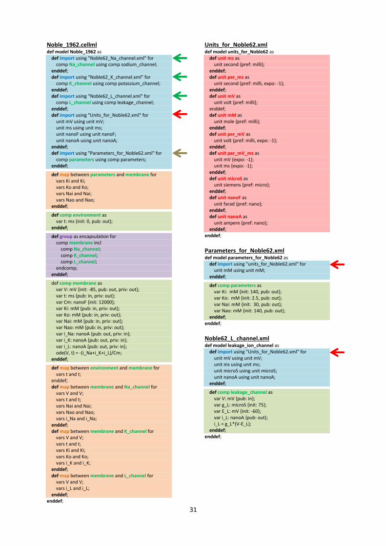
31

Noble_1962.cellml def model Noble_1962 as

def import using "Noble62_Na_channel.xml" for

comp Na_channel using comp sodium_channel;

enddef; def import using "Noble62_K_channel.xml" for

comp K_channel using comp potassium_channel;

enddef; def import using "Noble62_L_channel.xml" for

comp L_channel using comp leakage_channel;

enddef; def import using "Units_for_Noble62.xml" for

unit mV using unit mV;

unit ms using unit ms;

unit nanoF using unit nanoF;

unit nanoA using unit nanoA;

enddef; def import using "Parameters_for_Noble62.xml" for

comp parameters using comp parameters;

enddef;

def map between parameters and membrane for

vars Ki and Ki;

vars Ko and Ko;

vars Nai and Nai;

vars Nao and Nao;

enddef;

def comp environment as

var t: ms {init: 0, pub: out};

enddef;

def group as encapsulation for

comp membrane incl

comp Na_channel; comp K_channel; comp L_channel; endcomp;

enddef;

def comp membrane as

var V: mV {init: -85, pub: out, priv: out};

var t: ms {pub: in, priv: out};

var Cm: nanoF {init: 12000};

var Ki: mM {pub: in, priv: out};

var Ko: mM {pub: in, priv: out};

var Nai: mM {pub: in, priv: out};

var Nao: mM {pub: in, priv: out};

var i_Na: nanoA {pub: out, priv: in};

var i_K: nanoA {pub: out, priv: in};

var i_L: nanoA {pub: out, priv: in};

ode(V, t) = -(i_Na+i_K+i_L)/Cm;

enddef;

def map between environment and membrane for

vars t and t;

enddef;

def map between membrane and Na_channel for

vars V and V;

vars t and t;

vars Nai and Nai;

vars Nao and Nao;

vars i_Na and i_Na;

enddef; def map between membrane and K_channel for

vars V and V;

vars t and t;

vars Ki and Ki;

vars Ko and Ko;

vars i_K and i_K;

enddef; def map between membrane and L_channel for

vars V and V;

vars i_L and i_L;

enddef; enddef;

Units_for_Noble62.xml def model units_for_Noble62 as

def unit ms as

unit second {pref: milli};

enddef; def unit per_ms as

unit second {pref: milli, expo: -1};

enddef; def unit mV as

unit volt {pref: milli};

enddef;

def unit mM as

unit mole {pref: milli};

enddef; def unit per_mV as

unit volt {pref: milli, expo: -1};

enddef; def unit per_mV_ms as

unit mV {expo: -1};

unit ms {expo: -1};

enddef; def unit microS as

unit siemens {pref: micro};

enddef; def unit nanoF as

unit farad {pref: nano};

enddef; def unit nanoA as

unit ampere {pref: nano};

enddef; enddef;

Parameters_for_Noble62.xml def model parameters_for_Noble62 as

def import using "units_for_Noble62.xml" for

unit mM using unit mM;

enddef;

def comp parameters as

var Ki: mM {init: 140, pub: out};

var Ko: mM {init: 2.5, pub: out};

var Nai: mM {init: 30, pub: out};

var Nao: mM {init: 140, pub: out};

enddef; enddef;

Noble62_L_channel.xml def model leakage_ion_channel as

def import using "Units_for_Noble62.xml" for

unit mV using unit mV;

unit ms using unit ms;

unit microS using unit microS;

unit nanoA using unit nanoA;

enddef;

def comp leakage_channel as

var V: mV {pub: in};

var g_L: microS {init: 75};

var E_L: mV {init: -60};

var i_L: nanoA {pub: out};

i_L = g_L*(V-E_L);

enddef; enddef;

32

Noble62_Na_channel.xml def model sodium_ion_channel as

def import using "Units_for_Noble62.xml" for

unit mV using unit mV;

unit ms using unit ms;

unit mM using unit mM;

unit per_ms using unit per_ms;

unit per_mV using unit per_mV;

unit per_mV_ms using unit per_mV_ms;

unit microS using unit microS;

unit nanoA using unit nanoA;

enddef;

def group as encapsulation for

comp sodium_channel incl

comp sodium_channel_m_gate;

comp sodium_channel_h_gate;

endcomp;

enddef;

def comp sodium_channel as

var V: mV {pub: in, priv: out};

var t: ms {pub: in, priv: out};

var g_Na_max: microS {init: 400000};

var g_Na: microS;

var E_Na: mV;

var m: dimensionless {priv: in};

var h: dimensionless {priv: in};

var Nai: mM {pub: in};

var Nao: mM {pub: in};

var RTF: mV {init: 25};

var i_Na: nanoA {pub: out};

E_Na = RTF*ln(Nao/Nai);

g_Na = pow(m, 3{dimensionless})*h*g_Na_max;

i_Na = (g_Na+140{microS})*(V-E_Na);

enddef;

def comp sodium_channel_m_gate as

var V: mV {pub: in};

var t: ms {pub: in};

var m: dimensionless {init: 0.01, pub: out};

var alpha_m: per_ms;

var beta_m: per_ms;

alpha_m = -0.10{per_mV_ms}*(V+48{mV})

/(exp(-(V+48{mV})/15{mV})-1{dimensionless});

beta_m = 0.12{per_mV_ms}*(V+8{mV})

/(exp((V+8{mV})/5{mV})-1{dimensionless});

ode(m, t)=alpha_m*(1{dimensionless}-m)-beta_m*m;

enddef;

def comp sodium_channel_h_gate as

var V: mV {pub: in};

var t: ms {pub: in};

var h: dimensionless {init: 0.8, pub: out};

var alpha_h: per_ms;

var beta_h: per_ms;

alpha_h = 0.17{per_ms}*exp(-(V+90{mV})/20{mV});

beta_h = 1.00{per_ms}

/(1{dimensionless}+exp(-(V+42{mV})/10{mV}));

ode(h, t) = alpha_h*(1{dimensionless}-h)-beta_h*h;

enddef;

def map between sodium_channel and sodium_channel_m_gate for

vars V and V;

vars t and t;

vars m and m;

enddef;

def map between sodium_channel and sodium_channel_h_gate for

vars V and V;

vars t and t;

vars h and h;

enddef; enddef;

Noble62_K_channel.xml def model potassium_ion_channel as

def import using "Units_for_Noble62.xml" for

unit mV using unit mV;

unit ms using unit ms;

unit mM using unit mM;

unit per_ms using unit per_ms;

unit per_mV using unit per_mV;

unit per_mV_ms using unit per_mV_ms;

unit microS using unit microS;

unit nanoA using unit nanoA;

enddef;

def group as encapsulation for

comp potassium_channel incl

comp potassium_channel_n_gate;

endcomp;

enddef;

def comp potassium_channel as

var V: mV {pub: in, priv: out};

var t: ms {pub: in, priv: out};

var n: dimensionless {priv: in};

var Ki: mM {pub: in};

var Ko: mM {pub: in};

var RTF: mV {init: 25};

var E_K: mV;

var g_K1: microS;

var g_K2: microS;

var i_K: nanoA {pub: out};

E_K = RTF*ln(Ko/Ki);

g_K1 = 1200{microS}*exp(-(V+90{mV})/50{mV})

+15{microS}*exp((V+90{mV})/60{mV});

g_K2 = 1200{microS}*pow(n, 4{dimensionless});

i_K = (g_K1+g_K2)*(V-E_K);

enddef;

def comp potassium_channel_n_gate as

var V: mV {pub: in};

var t: ms {pub: in};

var n: dimensionless {init: 0.01, pub: out};

var alpha_n: per_ms;

var beta_n: per_ms;

alpha_n = -0.0001{per_mV_ms}*(V+50{mV})

/(exp(-(V+50{mV})/10{mV})-1{dimensionless});

beta_n = 0.0020{per_ms}*exp(-(V+90{mV})/80{mV});

ode(n,t)= alpha_n*(1{dimensionless}-n)-beta_n*n;

enddef;

def map between environment

and potassium_channel for

vars V and V;

vars t and t;

enddef; def map between potassium_channel and

potassium_channel_n_gate for

vars V and V;

vars t and t;

vars n and n;

enddef; enddef;

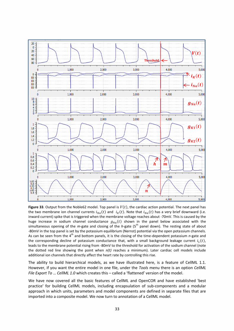
33

Figure 33. Output from the Noble62 model. Top panel is ( ), the cardiac action potential. The next panel has

the two membrane ion channel currents ( ) and ( ). Note that ( ) has a very brief downward (i.e.

inward current) spike that is triggered when the membrane voltage reaches about -70mV. This is caused by the

huge increase in sodium channel conductance ( ) shown in the panel below associated with the

simultaneous opening of the m-gate and closing of the h-gate (5th

panel down). The resting state of about

-80mV in the top panel is set by the potassium equilibrium (Nernst) potential via the open potassium channels.

As can be seen from the 4th

and bottom panels, it is the closing of the time-dependent potassium n-gate and

the corresponding decline of potassium conductance that, with a small background leakage current ( ), leads to the membrane potential rising from -80mV to the threshold for activation of the sodium channel (note

the dotted red line showing the point when n(t) reaches a minimum). Later cardiac cell models include

additional ion channels that directly affect the heart rate by controlling this rise.

The ability to build hierarchical models, as we have illustrated here, is a feature of CellML 1.1.

However, if you want the entire model in one file, under the Tools menu there is an option CellML File Export To … CellML 1.0 which creates this – called a ‘flattened’ version of the model.

We have now covered all the basic features of CellML and OpenCOR and have established 'best

practice' for building CellML models, including encapsulation of sub-components and a modular

approach in which units, parameters and model components are defined in separate files that are

imported into a composite model. We now turn to annotation of a CellML model.

𝑽(𝒕)

𝒊𝑵𝒂(𝒕) 𝒊𝑲(𝒕)

𝒈𝑵𝒂(𝒕)

𝒈𝑲𝟏(𝒕)

𝒈𝑲𝟐(𝒕)

𝒉 𝒎

𝒏

Threshold

34

12. Model annotation

One of the most powerful features of CellML is its ability to import models. This means that complex

models can be built up by combining previously defined models. There is a potential problem with

this process, however, since the imported models (often developed by completely different

modellers) may represent the same biological or biophysical entity with different expressions. The

potassium channel model in Section 8, for example, represents the intracellular concentration of

potassium as ‘Ki’ (see the CellML Text code on page 17) but another model involving the intracellular

potassium concentration may use a different expression.

The solution to this dilemma is to annotate the CellML variables with names from controlled

vocabularies that have been agreed upon by the relevant scientific community. In this case we may

simply want to annotate Ki as ‘the concentration of potassium in the cytosol’. This expression, however, refers to three distinct entities: concentration, potassium and cytosol. We might also want

to specify that we are referring to the cytosol of a neuron … and that the neuron comes from a

particular part of a giant squid (the experimental animal used by Hodgkin and Huxley). Annotations

can clearly get very complicated!

What comes to our rescue here is that most scientific communities have developed controlled

vocabularies together with the relationships between the terms of that vocabulary – called

ontologies. Furthermore relationships can always be expressed in the form subject-predicate-object. E.g. Ki is-the-concentration-of potassium is one relationship and potassium in-the cytosol is

another. Each object can become the subject of another expression. We could continue, for

example, with cytosol of-the neuron, neuron of-the squid and so on. The terms is-the-concentration-of, in-the and of-the are the predicates and these semantically rich expressions too

have to come from controlled vocabularies. Each of these subject-predicate-object expressions is

called an RDF triple and the World Wide Web consortium39

has established a framework called the

Resource Description Framework (RDF40

) to support these.

CellML models therefore contain two parts, one dealing with syntax (the MathML definition of the

models together with the structure of components, connections, groups, units, etc) as discussed in

previous sections, and one dealing with semantics (the meanings of the terms used in the models)

discussed in this section41

. This latter is also referred to as metadata – i.e. data about data.

In the CellML metadata specification42

the first RDF subject of a triple is a CellML element (e.g. a

variable such as ‘Ki’), the RDF predicate is chosen from the Biomodels Biological Qualifiers43

list, and

the RDF object is a URI (the string of characters used to identify the name of a resource44

).

Establishing these RDF links to biological and biophysical meaning is the goal of annotation.

Note the different types of subject/object used in the RDF triples: the concentration is a biophysical

entity, potassium is a chemical entity, the cytosol is an anatomical entity. In fact, to cover all the

terminology used in the models, CellML uses five separate ontologies:

x ChEBI (Chemical Entities of Biological Interest) www.ebi.ac.uk/chebi

x GO (Gene Ontology) www.geneontology.org

x FMA (Foundation Model of Anatomy) fma.biostr.washington.edu/projects/fm/

x Cell type ontology code.google.com/p/cell-ontology

x OPB sbp.bhi.washington.edu/projects/the-ontology-of-physics-for-biology-opb

These ontologies are available through OpenCOR’s annotation facilities as explained below.

39

Referred to as W3C – see www.w3.org 40

www.w3.org/RDF 41

For details on the annotation plugin see opencor.ws/user/plugins/editing/CellMLAnnotationView.html 42

See www.cellml.org/specifications/metadata/ and www.cellml.org/specifications/metadata/mcdraft 43

http://co.mbine.org/standards/qualifiers 44

http://en.wikipedia.org/wiki/Uniform_resource_identifier

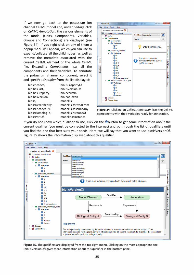
35

If we now go back to the potassium ion

channel CellML model and, under Editing, click

on CellML Annotation, the various elements of

the model (Units, Components, Variables,

Groups and Connections) are displayed (see

Figure 34). If you right click on any of them a

popup menu will appear, which you can use to

expand/collapse all the child nodes, as well as

remove the metadata associated with the

current CellML element or the whole CellML

file. Expanding Components lists all the

components and their variables. To annotate

the potassium channel component, select it

and specify a Qualifier from the list displayed:

bio:encodes, bio:isPropertyOf

bio:hasPart, bio:isVersionOf

bio:hasProperty, bio:occursIn

bio:hasVersion, bio:hasTaxon

bio:is, model:is

bio:isDescribedBy, model:isDerivedFrom

bio:isEncodedBy, model:isDescribedBy

bio:isHomologTo, model:isInstanceOf

bio:isPartOf, model:hasInstance

If you do not know which qualifier to use, click on the button to get some information about the

current qualifier (you must be connected to the internet) and go through the list of qualifiers until

you find the one that best suits your needs. Here, we will say that you want to use bio:isVersionOf.

Figure 35 shows the information displayed about this qualifier.

Figure 35. The qualifiers are displayed from the top right menu. Clicking on the most appropriate one

(bio:isVersionOf) gives more information about this qualifier in the bottom panel.

Figure 34. Clicking on CellML Annotation lists the CellML

components with their variables ready for annotation.

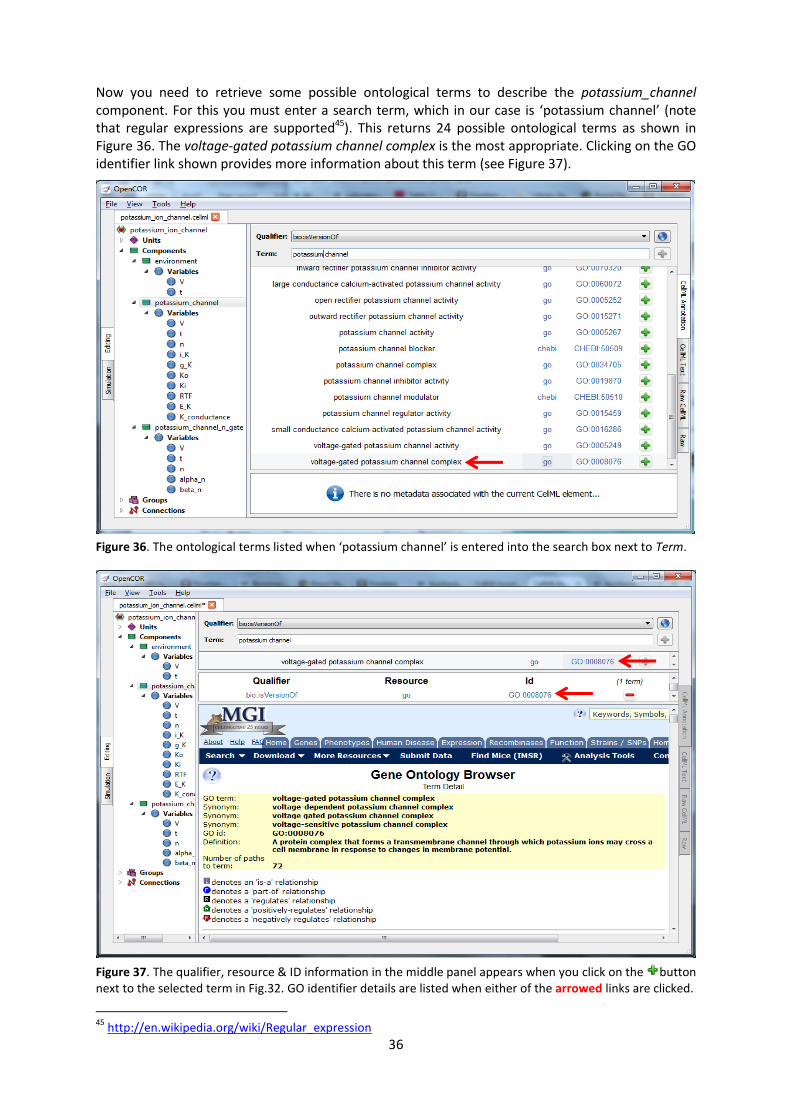
36

Now you need to retrieve some possible ontological terms to describe the potassium_channel component. For this you must enter a search term, which in our case is ‘potassium channel’ (note

that regular expressions are supported45

). This returns 24 possible ontological terms as shown in

Figure 36. The voltage-gated potassium channel complex is the most appropriate. Clicking on the GO

identifier link shown provides more information about this term (see Figure 37).

Figure 36. The ontological terms listed when ‘potassium channel’ is entered into the search box next to Term.

Figure 37. The qualifier, resource & ID information in the middle panel appears when you click on the button

next to the selected term in Fig.32. GO identifier details are listed when either of the arrowed links are clicked.

45

http://en.wikipedia.org/wiki/Regular_expression

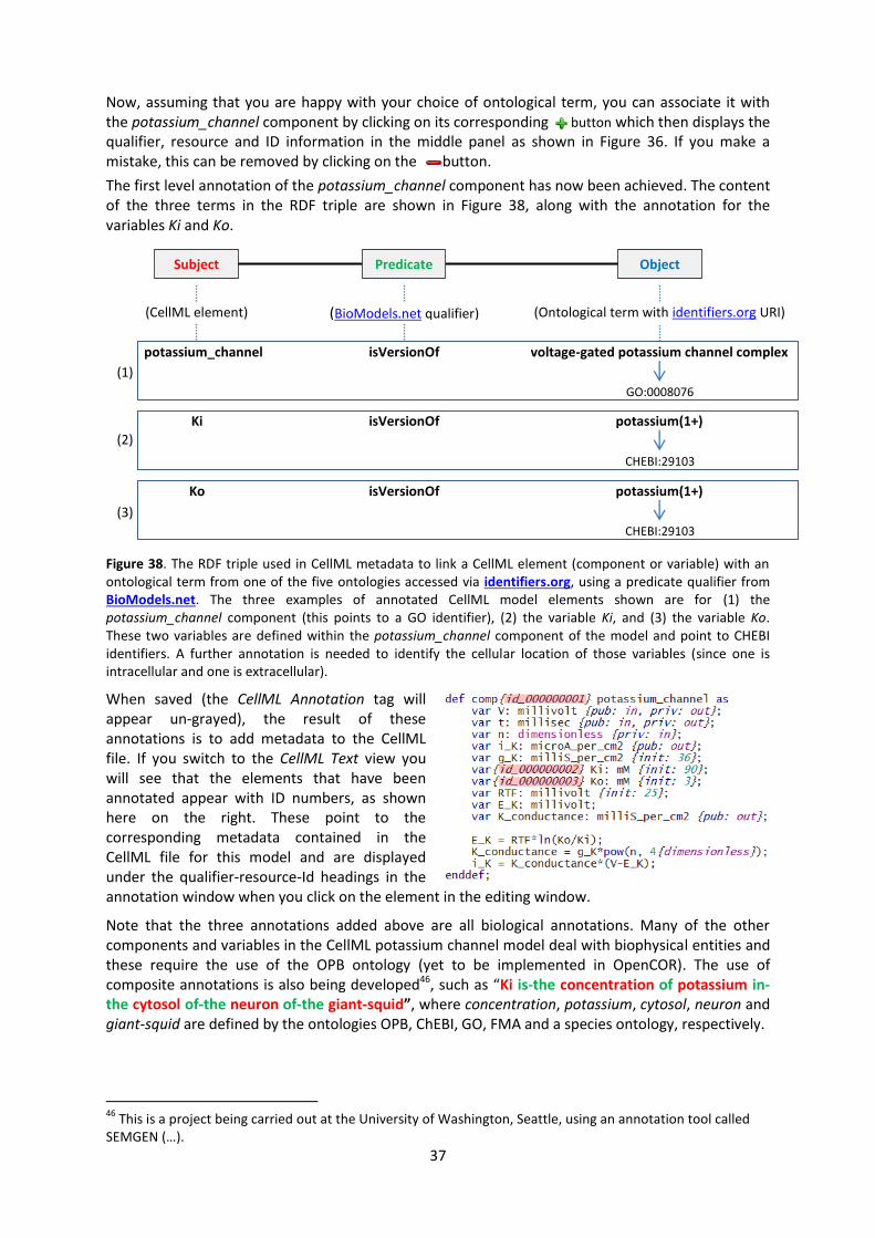
37

Now, assuming that you are happy with your choice of ontological term, you can associate it with

the potassium_channel component by clicking on its corresponding button which then displays the

qualifier, resource and ID information in the middle panel as shown in Figure 36. If you make a

mistake, this can be removed by clicking on the button.

The first level annotation of the potassium_channel component has now been achieved. The content

of the three terms in the RDF triple are shown in Figure 38, along with the annotation for the

variables Ki and Ko.

Figure 38. The RDF triple used in CellML metadata to link a CellML element (component or variable) with an

ontological term from one of the five ontologies accessed via identifiers.org, using a predicate qualifier from

BioModels.net. The three examples of annotated CellML model elements shown are for (1) the

potassium_channel component (this points to a GO identifier), (2) the variable Ki, and (3) the variable Ko.

These two variables are defined within the potassium_channel component of the model and point to CHEBI

identifiers. A further annotation is needed to identify the cellular location of those variables (since one is

intracellular and one is extracellular).

When saved (the CellML Annotation tag will

appear un-grayed), the result of these

annotations is to add metadata to the CellML

file. If you switch to the CellML Text view you

will see that the elements that have been

annotated appear with ID numbers, as shown

here on the right. These point to the

corresponding metadata contained in the

CellML file for this model and are displayed

under the qualifier-resource-Id headings in the

annotation window when you click on the element in the editing window.

Note that the three annotations added above are all biological annotations. Many of the other

components and variables in the CellML potassium channel model deal with biophysical entities and

these require the use of the OPB ontology (yet to be implemented in OpenCOR). The use of

composite annotations is also being developed46

, such as “Ki is-the concentration of potassium in-the cytosol of-the neuron of-the giant-squid”, where concentration, potassium, cytosol, neuron and

giant-squid are defined by the ontologies OPB, ChEBI, GO, FMA and a species ontology, respectively.

46

This is a project being carried out at the University of Washington, Seattle, using an annotation tool called

SEMGEN (…).

(1)

(2)

(3)

Subject

(CellML element)

Predicate

(BioModels.net qualifier)

qualifier

Object

(Ontological term with identifiers.org URI)

potassium_channel isVersionOf voltage-gated potassium channel complex

GO:0008076

Ki isVersionOf potassium(1+)

CHEBI:29103

Ko isVersionOf potassium(1+)

CHEBI:29103

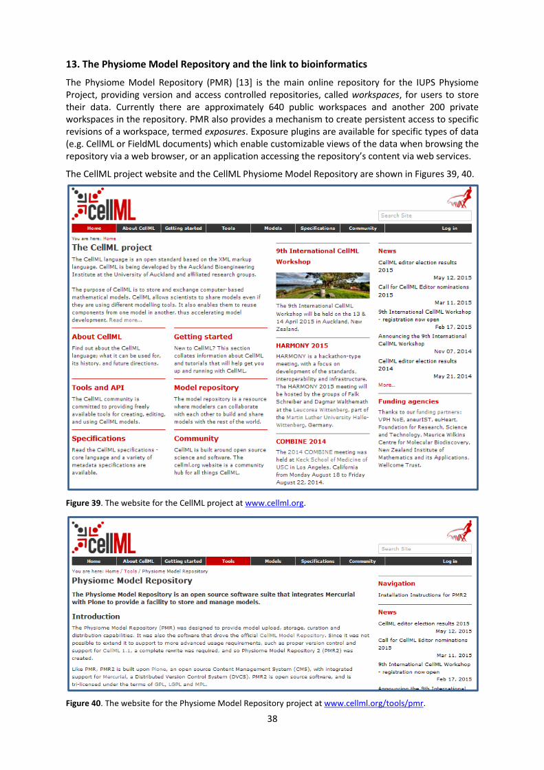
38

13. The Physiome Model Repository and the link to bioinformatics

The Physiome Model Repository (PMR) [13] is the main online repository for the IUPS Physiome

Project, providing version and access controlled repositories, called workspaces, for users to store

their data. Currently there are approximately 640 public workspaces and another 200 private

workspaces in the repository. PMR also provides a mechanism to create persistent access to specific

revisions of a workspace, termed exposures. Exposure plugins are available for specific types of data

(e.g. CellML or FieldML documents) which enable customizable views of the data when browsing the

repository via a web browser, or an application accessing the repository’s content via web services.

The CellML project website and the CellML Physiome Model Repository are shown in Figures 39, 40.

Figure 39. The website for the CellML project at www.cellml.org.

Figure 40. The website for the Physiome Model Repository project at www.cellml.org/tools/pmr.

39

The CellML models on models.physiomeproject.org are listed under 20 categories, shown below:

(numbers of exposures in each category are given besides the bar graph)

Browse by category x Calcium Dynamics 140

x Cardiovascular Circulation 60

x Cell Cycle 38

x Cell Migration 2

x Circadian Rhythms 22

x Electrophysiology 230

x Endocrine 60

x Excitation-Contraction Coupling 22

x Gene Regulation 12

x Hepatology 29

x Immunology 55

x Ion transport 13

x Mechanical Constitutive Laws 19

x Metabolism 86

x Myofilament Mechanics 22

x Neurobiology 33

x pH regulation 2

x PKPD 11

x Signal Transduction 120

x Synthetic Biology 6

Note that searching of models can be done anywhere on the site using the search box on the upper

right hand corner. An important benefit of ensuring that the models on the PMR are annotated is

that models can then be retrieved by a web-search using any of the annotated terms in the models.

To illustrate the features of PMR, click on the Hund, Rudy 2004 (Basic) model in the alphabetic listing

of models under Electrophysiology. This opens a web page (Figure 41) using a 32 character string

that has been randomly generated as the ID for the exposure page for that model.

Figure 41. The Physiome Model Repository exposure page for the basic Hund-Rudy 2004 model.

40

Note that the string is still unique even with only 5 characters:

e.g. https://models.physiomeproject.org/exposure/f4b71/hund_rudy_2004_a.cellml/view

The section labelled ‘Model Structure’ contains the journal paper abstract and often a diagram of

the model47

. This is shown for the Hund-Rudy 2004 model in Figure 42. This model, with over 22

separate protein model components, is also a good example of why it is important to build models

from modular components [14], and in particular the individual ion channels for electrophysiology

models.

Figure 42. A diagrammatic representation of the Hund-Rudy 2004 model.

There is a list of ‘Views Available’ for the CellMLmodel on the lower right hand side of the exposure

page. The function of each of these views is as follows:

Views Available Documentation - Takes you to the main exposure page.

Model Metadata - Lists metadata including authors, title, journal, Pubmed ID and model annotations.

Model Curation - Provides the curation status of the model. Note: this is soon to be updated.

Mathematics - Displays all the mathematical equations contained in the model.

Generated Code - Creates code (C, C-IDA, F77, MATLAB or Python) for the model.

Cite this model - Provides details on how to cite use of the CellML model.

Source view - Gives a full listing of the XML code for the model.

Simulate using OpenCell - This will be OpenCOR once the SED-ML API is included in OpenCOR.

Note that CellML models are available under a Creative Commons Attribution 3.0 Unported

License48

. This means that you are free to:

x Share — copy and redistribute the material in any medium or format

x Adapt — remix, transform, and build upon the material

for any purpose, including commercial use.

47

These are currently hand drawn SVG diagrams but the plan is to automatically generate them from the

model annotation and also (at some stage!) to animate them as the model is executed. 48

https://creativecommons.org/licenses/by/3.0/

41

The next stage of content development for PMR is to provide a list of the modular components of

these models each with their own exposure. For example, models for each of the individual ion

channels used in the publication-based electrophysiological models will be available as standalone

models that can then be imported as appropriate into a new composite model. Similarly for enzymes

in metabolic pathways and signalling complexes in signalling pathways, etc. Some examples of these

protein modules are:

Sodium/hydrogen exchanger 3 https://models.physiomeproject.org/e/236/

Thiazide-sensitive Na-Cl cotransporter https://models.physiomeproject.org/e/231/

Sodium/glucose cotransporter 1 https://models.physiomeproject.org/e/232/

Sodium/glucose cotransporter 2 https://models.physiomeproject.org/e/233/

Note that in each case, as well as the CellML-encoded mathematical model, links are provided (see

Figure 43) to the UniProt Knowledgebase for that protein, and to the Foundational Model of

Anatomy (FMA) ontology (via the EMBLE-EBI Ontology Lookup Service) for information about tissue

regions relevant to the expression of that protein (e.g. Proximal convoluted tubule, Apical plasma membrane; Epithelial cell of proximal tubule; Proximal straight tubule). Similar facilities are available

for SMBL-encoded biochemical reaction models through the Biomodels database [15].

Figure 43. The PMR workspace for the Thiazide-sensitive Na-Cl cotransporter. Bioinformatic data for this

model is accessed via the links under the headings highlight by the arrows and include Protein (labelled A) and

the model Location (labelled B). Other information is as already described for the Hund-Rudy 2004 model.

A B

42

14. Speed comparisons with MATLAB

Solution speed is important for complex computational models and here we compare the

performance of OpenCOR with MATLAB49

. Nine representative CellML models were chosen from

the PMR model repository. For the MATLAB tests we used the MATLAB code, generated

automatically from CellML, that is available on the PMR site. These comparisons are based on using

the default solvers (listed below) available in the two packages.

Testing environment

x MacBook Pro (Retina, Mid 2012).

x Processor: 2.6 GHz Intel Core i7.

x Memory: 16 GB 1600 MHz DDR3.

x Operating system: OS X Yosemite 10.10.3.

OpenCOR x Version: 0.4.1.

x Solver: CVODE with its default settings, except for its Maximum step parameter, which is set

to the model's stimulation duration, if needed.

MATLAB x Version: R2013a.

x Solver: ode15s (i.e. a solver suitable for stiff problems and which has low to medium order of

accuracy) with both its RelTol and AbsTol parameters set to 1e-7 and its MaxStep parameter

set to the stimulation duration, if needed.

Testing protocol x Run a model for a given simulation duration.

x Generate simulation data every milliseconds.

x Only keep track of all the simulation data (i.e. no graphical output).

x Run a model 7 times, discard the 2 slowest runs (to account for unpredictable slowdowns of

the testing machine) and average the resulting computational times.

x Computational times are obtained directly from OpenCOR and MATLAB (through a couple of

calls to cputime in the case of MATLAB).

Results

CellML model (from PMR on 18/6/2015)

Duration (s)

OpenCOR time (s)

MATLAB time (s)

Time ratio (MATLAB/OpenCOR)

Bondarenko et al. 2004 10 1.16 140.14 121

Courtemanche et al. 1998 * 100 0.998 45.720 46

Faber & Rudy 2000 50 0.717 29.010 40

Garny et al. 2003 100 0.996 48.180 48

Luo & Rudy 1991* 200 0.666 70.070 105

Noble 1962 1000 1.42 310.02 218

Noble et al. 1998 100 0.834 42.010 50

Nygren et al. 1998 100 0.824 31.370 38

ten Tusscher & Panfilov 2006 100 0.969 59.080 61

*The value of membrane.stim_end was increased so as to get action potentials for the duration of the simulation

Conclusions For this range of tests, OpenCOR is between 38 and 218 times faster than MATLAB.

A more extensive evaluation of these results is available on GitHub50

.

49

www.mathworks.com/products/matlab 50

https://github.com/opencor/speedcomparison. These tests were carried out by Alan Garny.

43

15. SED-ML, functional curation and Web Lab

In the same way that CellML models can be defined unambiguously, and shared easily, in a machine-

readable format, there is a need to do the same thing with 'protocols' – i.e. to define what you have

to do to replicate/simulate an experiment, and to analyse the results. An XML standard for this

called SED-ML51

is being developed by the CellML/SBML community and the API for SED-ML will

implemented in the next full version release of OpenCOR in order to allow precise and reproducible

control over the OpenCOR simulation and graphical output. This will also facilitate the curation of

models according to their functional behaviour under a range of experimental scenarios.

The key idea behind functional curation is that, when mathematical and computational models are

being developed, a primary goal should be the continuous comparison of those models against

experimental data. When computational models are being re-used in new studies, it is similarly

important to check that they behave appropriately in the new situation to which you're applying

them. To achieve this goal, a pre-requisite is to be able to replicate in-silico precisely the same

protocols used in an experiment of interest. A language for describing rich 'virtual experiment'

protocols and software for running these on compatible models is being developed in the

Computational Biology Group at Oxford University52

.

An online system called Web Lab53

is also being developed that supports definition of experimental

protocols for cardiac electrophysiology, and allows any CellML model to be tested under these

protocols [16]. This enables comparison of the behaviours of cellular models under different

experimental protocols: both to characterise a model’s behaviour, and comparing hypotheses by seeing how different models react under the same protocol (Figure 44).

Figure 44. A schematic of the way we organise model and protocol descriptions. Web Lab provides an interface

to a Model/Protocol Simulator, storing and displaying the results for cardiac electrophysiology models.

(Adapted from [16]).

The Web Lab website provides tools for comparing how two different cardiac electrophysiology

models behave under the same experimental protocols. Note that Web Lab demonstration for

CellML models of cardiac electrophysiology is a prototype for a more general approach to defining

simulation protocols for all CellML models.

51

The ‘Simulation Experiment Description Markup Language’: sed-ml.org 52

travis.cs.ox.ac.uk/FunctionalCuration/about.html This initiative is led by Jonathan Cooper and Gary Mirams. 53

travis.cs.ox.ac.uk/FunctionalCuration.

44

16. Future developments

Both CellML and OpenCOR are continuing to be developed. These notes will be updated to reflect

new features of both. The next release of OpenCOR (0.5) will include

¾ the SED-ML API which means that all the variables controlling the simulation and its output

can be specified in a file for that simulation

¾ the BioSignalML API which will allow experimental data to be read into OpenCOR in a

standardised way

¾ colour plots, to better distinguish overlapping traces in the output windows

Priorities for later releases of OpenCOR include the incorporation of GIT into OpenCOR to enable the

upload of models to PMR, graphical rendering of the model structure (using SVG), model building

templates, such as templates for creating Markov models, tools for parameter estimation and tools

for analysing model outputs.

The next release of CellML (1.2) will include the ability to specify a probability distribution for a

parameter value. Together with SED-ML, this will allow OpenCOR to generate error bounds on the

solutions, corresponding to the specified parameter uncertainty.

These notes are currently being extended to include

¾ a discussion of system identification and parameter estimation

¾ more extensive discussion of membrane protein models along the lines of the discussion on

page 41 of Section 13, and the creation of a PMR library of these models

¾ CellML modules for signal transduction pathways

45

References 1. Garny A and Hunter PJ. OpenCOR: OpenCOR: a modular and interoperable approach to

computational biology. Frontiers in Physiology 6, 26 (2015).

2. Cuellar AA, Lloyd CM, Nielsen PF, Halstead MDB, Bullivant DP, Nickerson DP and Hunter PJ.

An overview of CellML 1.1, a biological model description language. SIMULATION: Transactions of the Society for Modeling and Simulation 79(12):740-747, 2003

3. Yu T et al. The Physiome Model Repository 2. Bioinformatics 27, 743–744, 2011.

4. Hunter PJ. The IUPS Physiome Project: a framework for computational physiology. Progress in Biophysics and Molecular Biology 85, 551–569, 2004.

5. See www.cellml.org/about/publications for a more extensive list of publications on CellML and

OpenCOR.

6. Christie R, Nielsen PMF, Blackett S, Bradley C and Hunter PJ. FieldML: concepts and

implementation. Philosophical Transactions of the Royal Society (London) A367(1895):1869-

1884, 2009.

7. Britten RD, Christie GR, Little C, Miller AK, Bradley C, Wu A, Yu T, Hunter P, Nielsen P. FieldML, a

proposed open standard for the Physiome project for mathematical model representation. Med Biol Eng Comput 51(11), 1191-1207, 2013.

8. Hunter PJ et al. A vision and strategy for the virtual physiological human: 2012 update. Interface Focus 3, 2013. http://journal.frontiersin.org/article/10.3389/fphys.2015.00026/abstract

9. Thompson JMT and Stewart HB. Nonlinear Dynamics and Chaos, 2nd

Edn. Wiley, 2002.

10. Hodgkin AL and Huxley AF. A quantitative description of membrane current and its application to

conduction and excitation in nerve. Journal of Physiology 117, 500-544, 1952. PubMed ID:

12991237

11. Wigglesworth J. ‘Energy and Life’, Taylor & Francis Ltd, 1997.

12. Noble D. A modification of the Hodgkin-Huxley equations applicable to Purkinje fibre action and

pace-maker potentials. Journal of Physiology 160, 317-352, 1962.

13. Lloyd CM, Lawson JR, Hunter PJ and Nielsen PF. The CellML Model Repository. Bioinformatics 24,

2122-2123, 2008.

14. Cooling M, Hunter PJ and Crampin EJ. Modeling biological modularity with CellML. IET Systems Biology 2(2):73-79, 2008.

15. www.biomodels.org

16. Cooper J, Vik JO, Waltemath D. A call for virtual experiments: Accelerating the scientific process.

Progress in Biophysics and Molecular Biology 117, 99–106, 2015.