San Jose State University San Jose State University

SJSU ScholarWorks SJSU ScholarWorks

Master's Theses Master's Theses and Graduate Research

Spring 2020

Methods for Sensitive Detection of Magneto Optic Kerr Effect Methods for Sensitive Detection of Magneto Optic Kerr Effect

James Creed San Jose State University

Follow this and additional works at: https://scholarworks.sjsu.edu/etd_theses

Recommended Citation Recommended Citation Creed, James, "Methods for Sensitive Detection of Magneto Optic Kerr Effect" (2020). Master's Theses. 5092. DOI: https://doi.org/10.31979/etd.8brz-y9ww https://scholarworks.sjsu.edu/etd_theses/5092

This Thesis is brought to you for free and open access by the Master's Theses and Graduate Research at SJSU ScholarWorks. It has been accepted for inclusion in Master's Theses by an authorized administrator of SJSU ScholarWorks. For more information, please contact scholarworks@sjsu.edu.

METHODS FOR SENSITIVE DETECTION OF MAGNETO OPTIC

KERR EFFECT

A Thesis

Presented to

The Faculty of the Department of Physics & Astronomy

San Jose State University

In Partial Fulfillment

of the Requirements for the Degree

Master of Science

by

James K. Creed

May 2020

c© 2020

James K. Creed

ALL RIGHTS RESERVED

The Designated Thesis Committee Approves the Thesis Titled

METHODS FOR SENSITIVE DETECTION OF MAGNETO OPTICKERR EFFECT

by

James K. Creed

APPROVED FOR THE DEPARTMENT OF PHYSICS & ASTRONOMY

SAN JOSE STATE UNIVERSITY

May 2020

Dr. Peter Beyersdorf Department of Physics and Astronomy

Dr. Chris Smallwood Department of Physics and Astronomy

Dr. Ranko Heindl Department of Physics and Astronomy

ABSTRACT

METHODS FOR SENSITIVE DETECTION OF MAGNETO OPTICKERR EFFECT

by James K. Creed

The focus of this project is to numerically model the phenomenon known as

the Magneto Optic Kerr Effect, MOKE, where the interaction between light and

surface in the presence of a magnetic field, results in a rotation of the polarization

axis of the reflected light, and to develop a method by which to experimentally

measure the strength of the interaction. The amount of polarization rotation is

proportional to the strength of the magnetic field and changes in polarization can be

detected using polarizing optics. This thesis project successfully develops a

numerical model for MOKE and an experimental method is outlined in order to

measure the change in intensity using polarizing optics.

DEDICATION

I would like to dedicate this to my parents, Debbie and Kevin Creed without

whom I wouldn’t have the deepest love for science that I do and my wife Sarah Creed

who has supported me throughout so many years and made me believe that I can do

whatever I set my mind to.

v

ACKNOWLEDGEMENTS

I would like to also thank my SJSU professors for putting up with me and

getting me through school. Dr. Peter Beyersdorf, Dr. Ranko Heindl, Dr. Chris

Smallwood, Dr. Hamill, Dr. Wharton and Dr. Switz.

vi

TABLE OF CONTENTS

CHAPTER

1 INTRODUCTION TO THESIS 1

2 THEORY/BACKGROUND 2

2.1 Magneto-Optics . . . . . . . . . . . . . . . . . . . . . . . . . . . . . . 2

2.2 Jones Calculus . . . . . . . . . . . . . . . . . . . . . . . . . . . . . . 4

2.2.1 MOKE Material as Jones Matrix . . . . . . . . . . . . . . . . 5

2.3 Maxwell’s Equations at a Non-Magnetic Boundary . . . . . . . . . . . 7

2.3.1 Gauss’ Law . . . . . . . . . . . . . . . . . . . . . . . . . . . . 7

2.3.2 Faraday’s Law . . . . . . . . . . . . . . . . . . . . . . . . . . . 8

2.3.3 Gauss’ Law for Magnetism . . . . . . . . . . . . . . . . . . . . 9

2.3.4 Ampere’s Law . . . . . . . . . . . . . . . . . . . . . . . . . . . 9

2.3.5 Boundary Conditions: Summary . . . . . . . . . . . . . . . . . 10

2.4 Applying the Boundary Conditions . . . . . . . . . . . . . . . . . . . 10

2.4.1 S-Polarized Incident Light . . . . . . . . . . . . . . . . . . . . 11

2.4.2 p-polarized Incident Light . . . . . . . . . . . . . . . . . . . . 12

2.5 Maxwell Equations at Magnetic Interface . . . . . . . . . . . . . . . . 13

2.5.1 Air Glass Interface . . . . . . . . . . . . . . . . . . . . . . . . 17

2.6 Measuring Phase as Variations in Intensity . . . . . . . . . . . . . . . 21

2.6.1 Half Wave Plate: Major Axis of Polarization Rotation . . . . . 21

2.6.2 Quarter Wave Plate: Circular to Linear Polarization Conversion 22

vii

3 NUMERICAL MODEL IN PYTHON 24

3.0.1 Numerical Calculation Methods . . . . . . . . . . . . . . . . . 25

3.1 Results of Python Code . . . . . . . . . . . . . . . . . . . . . . . . . 26

3.2 Sensitivity Analysis . . . . . . . . . . . . . . . . . . . . . . . . . . . . 30

3.3 Sensitivity Improvements . . . . . . . . . . . . . . . . . . . . . . . . . 33

3.3.1 Balanced Detection . . . . . . . . . . . . . . . . . . . . . . . . 33

3.3.2 Modulated Detection . . . . . . . . . . . . . . . . . . . . . . . 34

4 FUTURE WORK: EXPERIMENT 35

4.1 Polarization Measurement System . . . . . . . . . . . . . . . . . . . . 35

4.2 Interpreting Results . . . . . . . . . . . . . . . . . . . . . . . . . . . . 36

4.3 Imaging System Design . . . . . . . . . . . . . . . . . . . . . . . . . . 36

5 CONCLUSION 39

APPENDIX

A APPENDIX 40

A.1 PyJones . . . . . . . . . . . . . . . . . . . . . . . . . . . . . . . . . . 40

A.2 Python Code . . . . . . . . . . . . . . . . . . . . . . . . . . . . . . . 41

A.3 Surface Plot . . . . . . . . . . . . . . . . . . . . . . . . . . . . . . . . 42

BIBLIOGRAPHY 44

viii

LIST OF TABLES

Table

2.1 Jones Matrices and Vectors . . . . . . . . . . . . . . . . . . . . . . . 5

ix

LIST OF FIGURES

Figure

2.1 Polar (a), Longitudinal (b), Transverse (c) MOKE Geometries . . . . 3

2.2 Boundary condition using Gauss’ Law . . . . . . . . . . . . . . . . . . 7

2.3 Boundary condition using Faraday’s Law . . . . . . . . . . . . . . . . 8

2.4 Reflection and transmission at an air glass interface using calculations

of equations 2.7 and 2.8 . . . . . . . . . . . . . . . . . . . . . . . . . 17

2.5 s-polarized vs. Incident Angle: Polar orientation . . . . . . . . . . . . 19

2.6 s-polarized Versus Incident Angle: Longitudinal orientation . . . . . . 19

2.7 p-polarized versus Incident Angle: polar orientation ; Calculated from

the Fresnel boundary equations for Polar orientation . . . . . . . . . 20

2.8 p-polarized Versus Incident Angle: longitudinal orientation ; Calcu-

lated from the Fresnel boundary equations for Longitudinal orientation 20

3.1 Optical experiment that is being modeled in Python . . . . . . . . . . 25

3.2 Intensity vs. Quarter Wave-Plate Angle: P Polarization . . . . . . . . 27

3.3 Intensity vs. Wave-Plate Angle: S Polarization . . . . . . . . . . . . . 27

3.4 S and p-polarized Versus Q: Longitudinal orientation . . . . . . . . . 28

3.5 S and p-polarized Versus Q: Polar orientation . . . . . . . . . . . . . 29

3.6 Changes in Intensity with Increasing Magnetic Field . . . . . . . . . . 30

4.1 Imaging Optics . . . . . . . . . . . . . . . . . . . . . . . . . . . . . . 38

x

CHAPTER 1

INTRODUCTION TO THESIS

This thesis project studies and models the interaction between light and

magnetic fields. Specifically, the focus of this thesis is to model the rotation of the

major axis of polarization of light after a reflection off of a metallic material that is

in the presence of a magnetic field. This effect is known as the Magneto Optic Kerr

Effect, MOKE, for short, and was discovered by John Kerr in 1877. MOKE is the

rotation of the major axis of polarization of light upon reflection from a

magnetically active material in the presence of a magnetic field. The amount of

rotation is proportional to the strength of the applied magnetic field. If an optical

system is designed to measure polarization rotations by changes in intensity, then it

is possible to measure the amount of intensity change due to MOKE. This thesis

project numerically models the MOKE phenomenon in Python and develops an

experimental method by which to detect the change in intensity due to MOKE.

2

CHAPTER 2

THEORY/BACKGROUND

2.1 Magneto-Optics

The term magneto-optics refers to the interaction between light and a magnetic

field and how magnetic fields can be utilized to manipulate properties of light.

MOKE is one specific interaction where the effect rotates the major axis of

polarization of light after reflecting off of a MOKE sample in the presence of a

magnetic field. A MOKE sample is a material that in the presence of a magnetic

field, exhibits MOKE. For example, a thin film of nickel will is a material when in

the presence of a magnetic field, will exhibit MOKE. John Kerr describes this effect

as a rotation of the polarization axis in the opposite direction of the magnetizing

current [2]. There are two effects that emerge when light reflects off of a magnetic

surface namely magnetic circular birefringence and magnetic circular dichroism. The

former is a difference in the index of refraction of the magnetic material, and the

latter refers to the difference in amount of absorption depending on the polarization

state. Magnetic circular dichroism converts linearly polarized light into elliptical

polarization by means of introducing a phase delay between the polarization

components. Circular birefringence rotates the major axis of polarization by

delaying both components equally. These effects scale with the strength of the

applied magnetic field however, these effects do not have equal magnitudes. The

dominating effect is the rotation of the major axis of polarization and only a slight

change in ellipticity for oblique incident light [2]. The focus of this thesis will be on

modeling the rotation of the major axis of polarization which is measured by an

3

optical system that converts changes in polarization to changes in intensity.

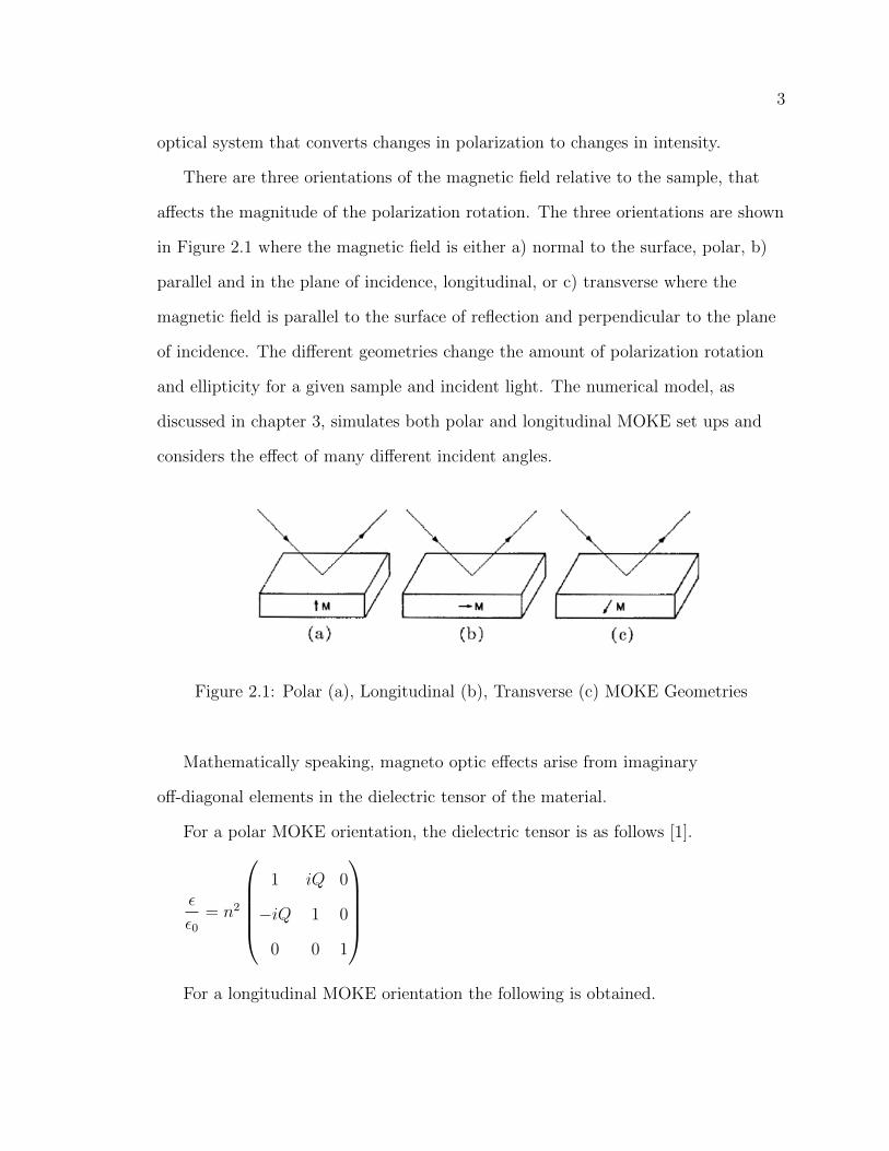
There are three orientations of the magnetic field relative to the sample, that

affects the magnitude of the polarization rotation. The three orientations are shown

in Figure 2.1 where the magnetic field is either a) normal to the surface, polar, b)

parallel and in the plane of incidence, longitudinal, or c) transverse where the

magnetic field is parallel to the surface of reflection and perpendicular to the plane

of incidence. The different geometries change the amount of polarization rotation

and ellipticity for a given sample and incident light. The numerical model, as

discussed in chapter 3, simulates both polar and longitudinal MOKE set ups and

considers the effect of many different incident angles.

Figure 2.1: Polar (a), Longitudinal (b), Transverse (c) MOKE Geometries

Mathematically speaking, magneto optic effects arise from imaginary

off-diagonal elements in the dielectric tensor of the material.

For a polar MOKE orientation, the dielectric tensor is as follows [1].

ε

ε0= n2

1 iQ 0

−iQ 1 0

0 0 1

For a longitudinal MOKE orientation the following is obtained.

4

ε

ε0= n2

1 0 −iQ

0 1 0

iQ 0 1

Where Q is a magnetic parameter that is proportional to the strength of the

magnetic field and dependent on the properties of the material. n is the average

index of refraction of the material. The off-diagonal elements are what give rise to

the changes in polarization by affecting the phase of the polarization components of

light.

2.2 Jones Calculus

The mathematical basis used to model the behavior of the components in the

experiment and model the outcome of the experiment is known as Jones calculus.

Jones calculus, is the mathematical formulation by which optical elements are

defined as matrices, known as Jones matrices, that perform a coordinate rotation on

the polarization components of the incident light which is represented by a Jones

vector. To compute the end polarization state or intensity of the light after passing

through a series of optics is a series of matrix multiplications, resulting in a 2x1

vector matrix representing the electric field polarization. Squaring this vector results

in a vector representing the intensity. Below are the relevant Jones vectors and

matrices used in this experiment and later in the paper, I will go into some sample

calculations that demonstrate how to use Jones calculus as well as how some of these

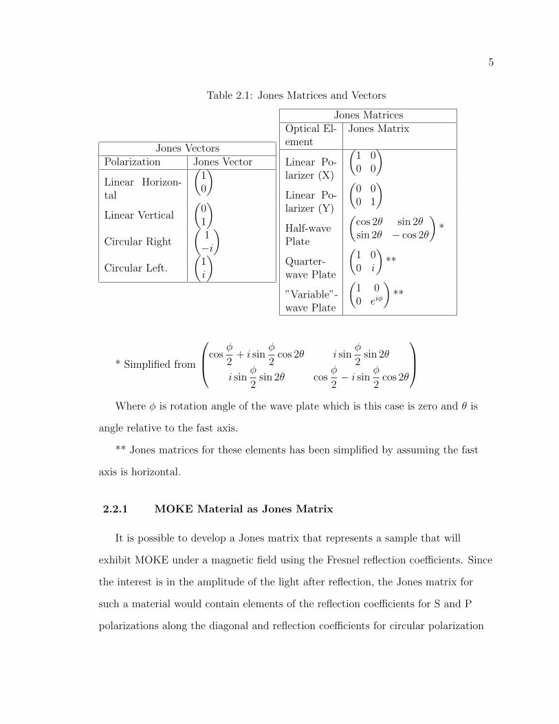
optical elements will be used. Table 2.1 below, shows the relevant Jones matrices

and vectors for the given optical elements that are considered in the calculations.

5

Table 2.1: Jones Matrices and Vectors

Jones VectorsPolarization Jones Vector

Linear Horizon-tal

(10

)Linear Vertical

(01

)Circular Right

(1−i

)Circular Left.

(1i

)

Jones MatricesOptical El-ement

Jones Matrix

Linear Po-larizer (X)

(1 00 0

)Linear Po-larizer (Y)

(0 00 1

)Half-wavePlate

(cos 2θ sin 2θsin 2θ − cos 2θ

)*

Quarter-wave Plate

(1 00 i

)**

”Variable”-wave Plate

(1 00 eiφ

)**

* Simplified from

cosφ

2+ i sin

φ

2cos 2θ i sin

φ

2sin 2θ

i sinφ

2sin 2θ cos

φ

2− i sin

φ

2cos 2θ

Where φ is rotation angle of the wave plate which is this case is zero and θ is

angle relative to the fast axis.

** Jones matrices for these elements has been simplified by assuming the fast

axis is horizontal.

2.2.1 MOKE Material as Jones Matrix

It is possible to develop a Jones matrix that represents a sample that will

exhibit MOKE under a magnetic field using the Fresnel reflection coefficients. Since

the interest is in the amplitude of the light after reflection, the Jones matrix for

such a material would contain elements of the reflection coefficients for S and P

polarizations along the diagonal and reflection coefficients for circular polarization

6

states, a combination of S and P, on the off diagonal elements. Below is the

definition of the Jones matrix representing a MOKE material which has also been

derived in a paper by Zak et. al. [1].

MOKE Jones Matrix:

rss rsp

rps rpp

In a numerical model, these reflection coefficients can be calculated by applying

the boundary conditions as defined by Maxwell’s equations to an interface between

a non-magnetic, air, and a magnetic surface, the sample. Then solving the system of

equations for the Fresnel coefficients. The amount of polarization rotation due to

MOKE is also defined in terms of the Fresnel coefficients as the following.

For S-Polarized incident light: θKerr =rpsrss

for P - Polarized incident light: θKerr =rsprpp

Computationally the Fresnel coefficients will be solved for using the method laid

out by Zak et. al. and used to estimate the amount of rotation of the axis of

polarization and the intensity change due to MOKE assuming a completely ideal

system.

A general approach to evaluating the boundary conditions between a magnetic

and non magnetic material comes from a method developed by Zak et al. which has

been generalized to solve the boundary conditions between either a non-magnetic or

magnetic interface[1]. Since his method is general to any materials, applying it to an

interface where the results are well defined, e.g. air to glass, is done as a verification

that this method works as expected.

7

2.3 Maxwell’s Equations at a Non-Magnetic Boundary

The Fresnel coefficient equations come from applying Maxwell’s equations across

the interface of two materials. Let us walk through applying Maxwell’s equations

between two non-magnetic materials to understand the constraints that allow us to

solve for the Fresnel coefficients.

2.3.1 Gauss’ Law

Let’s start with applying Gauss’ Law across the interface. The first step is to

define a Gaussian loop between the interfaces of the materials which provide us with

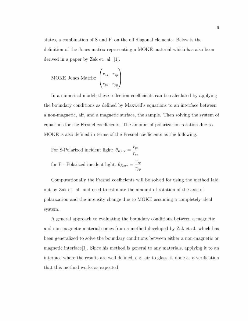
the behavior of the perpendicular component of the electric field. The boundary

condition is derived by applying Gauss’ Law, equation 2.1, across the boundary

shown in Figure 2.2

Figure 2.2: Boundary condition using Gauss’ Law

Starting with Gauss’ Law and expanding the equation to both sides of the

boundary [5]. ∮εE · dA = q (2.1)

8

The following expression is obtained by expanding Gauss’ law based on the fact

that the charge inside a dielectric is zero.

ε1E1⊥ − ε2E2⊥ = 0

Where E2⊥ and ε2 represent the perpendicular component of the electric field

and the permittivity of the second medium. Simplifying results in equation 2.2

below.

ε1E1⊥ = ε2E2⊥ (2.2)

The result here is that the perpendicular components of the electric field must

be equal across the boundary.

2.3.2 Faraday’s Law

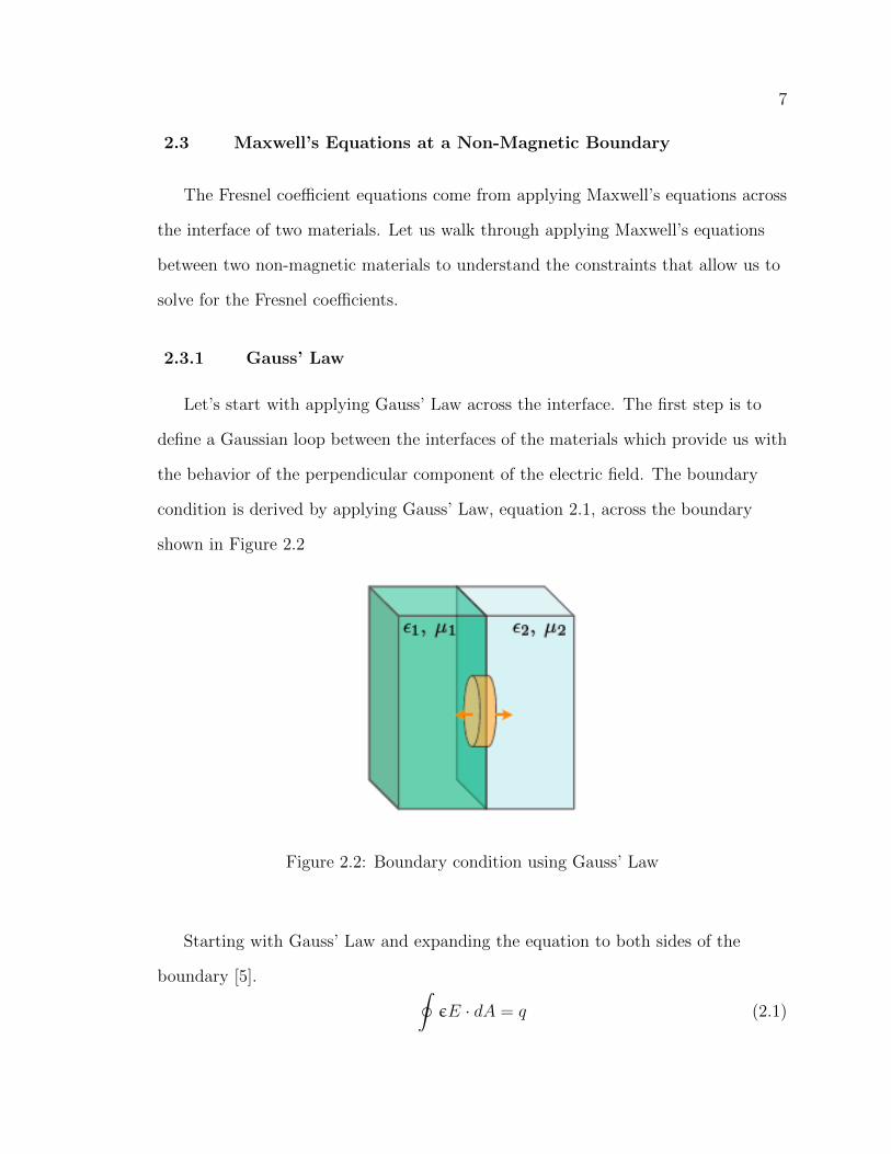
Applying Faraday’s at the interface will yield the relationship between the

parallel components of the electric field [5]. The boundary is shown below in Figure

2.3.

Figure 2.3: Boundary condition using Faraday’s Law

9

∮E · ds = − d

dt

∫B · dA

The area of the loop is infinitesimal so the right ride of Faraday’s law becomes

zero.

E1‖ = E2‖

Where E1‖ and E2‖ are the parallel components of the electric field of first and

second medium respectively. Applying Faraday’s law at the interface shows that the

parallel components of the electric field must be equal.

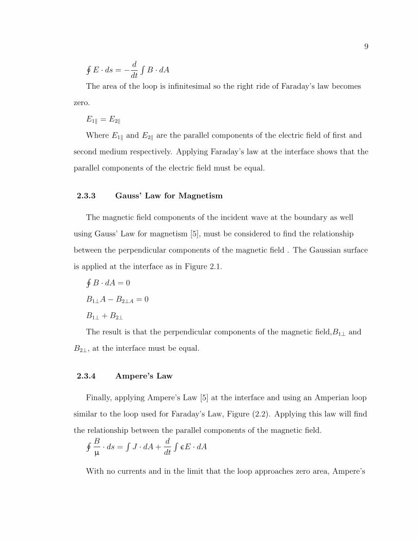
2.3.3 Gauss’ Law for Magnetism

The magnetic field components of the incident wave at the boundary as well

using Gauss’ Law for magnetism [5], must be considered to find the relationship

between the perpendicular components of the magnetic field . The Gaussian surface

is applied at the interface as in Figure 2.1.∮B · dA = 0

B1⊥A−B2⊥A = 0

B1⊥ +B2⊥

The result is that the perpendicular components of the magnetic field,B1⊥ and

B2⊥, at the interface must be equal.

2.3.4 Ampere’s Law

Finally, applying Ampere’s Law [5] at the interface and using an Amperian loop

similar to the loop used for Faraday’s Law, Figure (2.2). Applying this law will find

the relationship between the parallel components of the magnetic field.∮ Bµ· ds =

∫J · dA+

d

dt

∫εE · dA

With no currents and in the limit that the loop approaches zero area, Ampere’s

10

law reduces to the following.

B1‖

µ1

L−B2‖

µ2

L = 0

B1‖

µ1

=B2‖

µ2

Finally the last boundary condition constrains the parallel components of the

magnetic field to be equal at the interface.

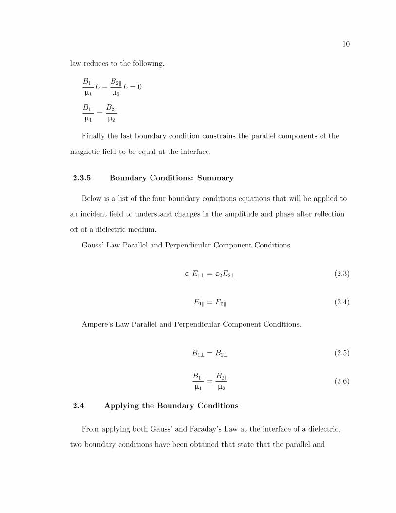
2.3.5 Boundary Conditions: Summary

Below is a list of the four boundary conditions equations that will be applied to

an incident field to understand changes in the amplitude and phase after reflection

off of a dielectric medium.

Gauss’ Law Parallel and Perpendicular Component Conditions.

ε1E1⊥ = ε2E2⊥ (2.3)

E1‖ = E2‖ (2.4)

Ampere’s Law Parallel and Perpendicular Component Conditions.

B1⊥ = B2⊥ (2.5)

B1‖

µ1

=B2‖

µ2

(2.6)

2.4 Applying the Boundary Conditions

From applying both Gauss’ and Faraday’s Law at the interface of a dielectric,

two boundary conditions have been obtained that state that the parallel and

11

perpendicular components of the electric field must be equal at the interface. Now

that the boundary conditions are defined, the next step is to solve for the Fresnel

coefficients for two interface cases. The first case is that of a non-magnetic material

interface and the second is a MOKE material in the presence of a magnetic field.

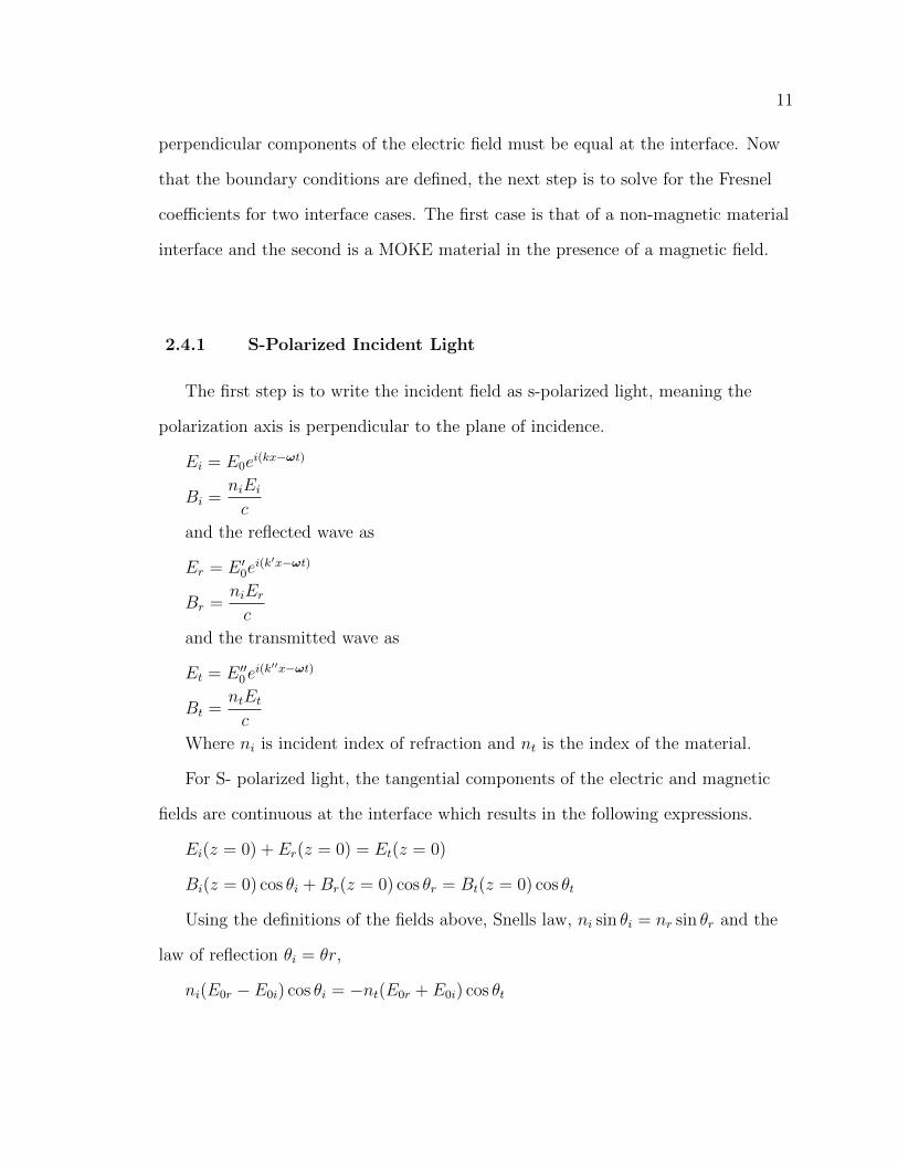
2.4.1 S-Polarized Incident Light

The first step is to write the incident field as s-polarized light, meaning the

polarization axis is perpendicular to the plane of incidence.

Ei = E0ei(kx−ωt)

Bi =niEic

and the reflected wave as

Er = E ′0ei(k′x−ωt)

Br =niErc

and the transmitted wave as

Et = E ′′0ei(k′′x−ωt)

Bt =ntEtc

Where ni is incident index of refraction and nt is the index of the material.

For S- polarized light, the tangential components of the electric and magnetic

fields are continuous at the interface which results in the following expressions.

Ei(z = 0) + Er(z = 0) = Et(z = 0)

Bi(z = 0) cos θi +Br(z = 0) cos θr = Bt(z = 0) cos θt

Using the definitions of the fields above, Snells law, ni sin θi = nr sin θr and the

law of reflection θi = θr,

ni(E0r − E0i) cos θi = −nt(E0r + E0i) cos θt

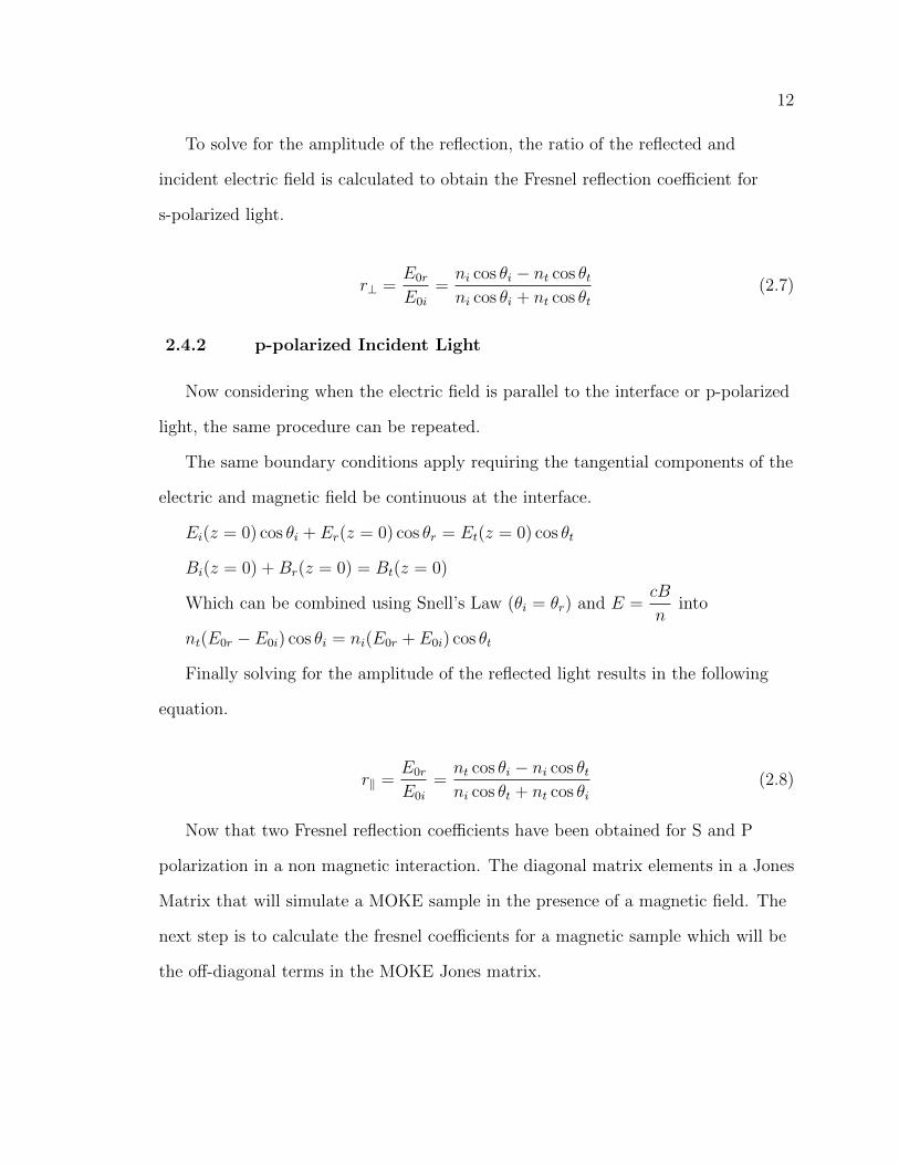
12

To solve for the amplitude of the reflection, the ratio of the reflected and

incident electric field is calculated to obtain the Fresnel reflection coefficient for

s-polarized light.

r⊥ =E0r

E0i

=ni cos θi − nt cos θtni cos θi + nt cos θt

(2.7)

2.4.2 p-polarized Incident Light

Now considering when the electric field is parallel to the interface or p-polarized

light, the same procedure can be repeated.

The same boundary conditions apply requiring the tangential components of the

electric and magnetic field be continuous at the interface.

Ei(z = 0) cos θi + Er(z = 0) cos θr = Et(z = 0) cos θt

Bi(z = 0) +Br(z = 0) = Bt(z = 0)

Which can be combined using Snell’s Law (θi = θr) and E =cB

ninto

nt(E0r − E0i) cos θi = ni(E0r + E0i) cos θt

Finally solving for the amplitude of the reflected light results in the following

equation.

r‖ =E0r

E0i

=nt cos θi − ni cos θtni cos θt + nt cos θi

(2.8)

Now that two Fresnel reflection coefficients have been obtained for S and P

polarization in a non magnetic interaction. The diagonal matrix elements in a Jones

Matrix that will simulate a MOKE sample in the presence of a magnetic field. The

next step is to calculate the fresnel coefficients for a magnetic sample which will be

the off-diagonal terms in the MOKE Jones matrix.

13

2.5 Maxwell Equations at Magnetic Interface

A new method must be applied when evaluating the Fresnel coefficients at a

boundary between a non-magnetic and magnetic surface. The dielectric term that is

used between two non-magnetic surfaces is a scalar value since the dielectric

constant does not change depending on the spatial direction the light travels in the

second material. However, in a magnetic material, the dielectric constant becomes a

tensor where the direction of propagation will change the value the dielectric

“constant”. Applying the method developed by Zak et al follows a generalized

procedure, where a matrix representing the magnetic material is used when

evaluating the boundary conditions at the interface[1]. The incoming light is

represented by a 4x1 vector whose elements are the polarization states. Doing so

writes the polarization states in the basis of a MOKE material in the presence of a

magnetic field which in this case is combinations of right and left circular

polarization states. Evaluating the boundary conditions then returns a set of four

independent equations that can be solved for the Fresnel coefficients which allows us

to populate a 4x4 matrix containing the Fresnel coefficients in the basis of the

polarization states. This process is applied for both polar and longitudinal MOKE

geometries where the corresponding medium matrix is used in the calculations.

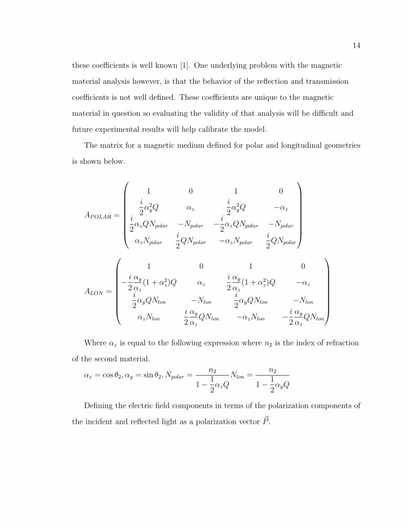
Below is the medium matrix for a magnetic and non-magnetic material, as

derived by Zak et al. [1], for polar and longitudinal geometries which contains

variables dependent on the incident angle of light, the index of refraction of each

material and the magnetic parameter, Q. Setting Q = 0 will result in a medium

matrix representing a non-magnetic material which in this experiment would be air.

Later in this analysis, the validity of the method laid out by Zak et al., by

evaluating the Fresnel coefficients at an air-glass interface where the behavior of

14

these coefficients is well known [1]. One underlying problem with the magnetic

material analysis however, is that the behavior of the reflection and transmission

coefficients is not well defined. These coefficients are unique to the magnetic

material in question so evaluating the validity of that analysis will be difficult and

future experimental results will help calibrate the model.

The matrix for a magnetic medium defined for polar and longitudinal geometries

is shown below.

APOLAR =

1 0 1 0

i

2α2yQ αz

i

2α2yQ −αz

i

2αzQNpolar −Npolar − i

2αzQNpolar −Npolar

αzNpolari

2QNpolar −αzNpolar

i

2QNpolar

ALON =

1 0 1 0

− i2

αyαz

(1 + α2z)Q αz

i

2

αyαz

(1 + α2z)Q −αz

i

2αyQNlon −Nlon

i

2αyQNlon −Nlon

αzNloni

2

αyαzQNlon −αzNlon − i

2

αyαzQNlon

Where αz is equal to the following expression where n2 is the index of refraction

of the second material.

αz = cos θ2, αy = sin θ2, Npolar =n2

1− 1

2αzQ

Nlon =n2

1− 1

2αyQ

Defining the electric field components in terms of the polarization components of

the incident and reflected light as a polarization vector ~P .

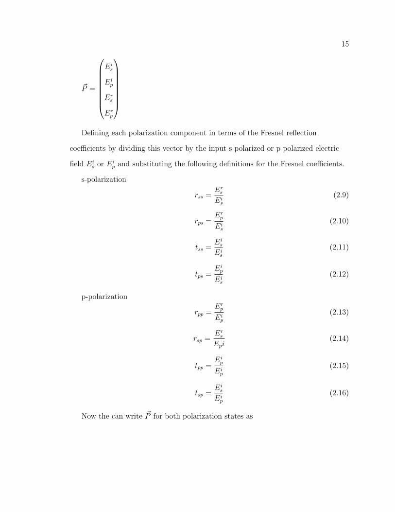
15

~P =

Eis

Eip

Ers

Erp

Defining each polarization component in terms of the Fresnel reflection

coefficients by dividing this vector by the input s-polarized or p-polarized electric

field Eis or Ei

p and substituting the following definitions for the Fresnel coefficients.

s-polarization

rss =Ers

Eis

(2.9)

rps =Erp

Eis

(2.10)

tss =Eis

Eis

(2.11)

tps =Eip

Eis

(2.12)

p-polarization

rpp =Erp

Eip

(2.13)

rsp =Ers

Epi(2.14)

tpp =Eip

Eip

(2.15)

tsp =Eis

Eip

(2.16)

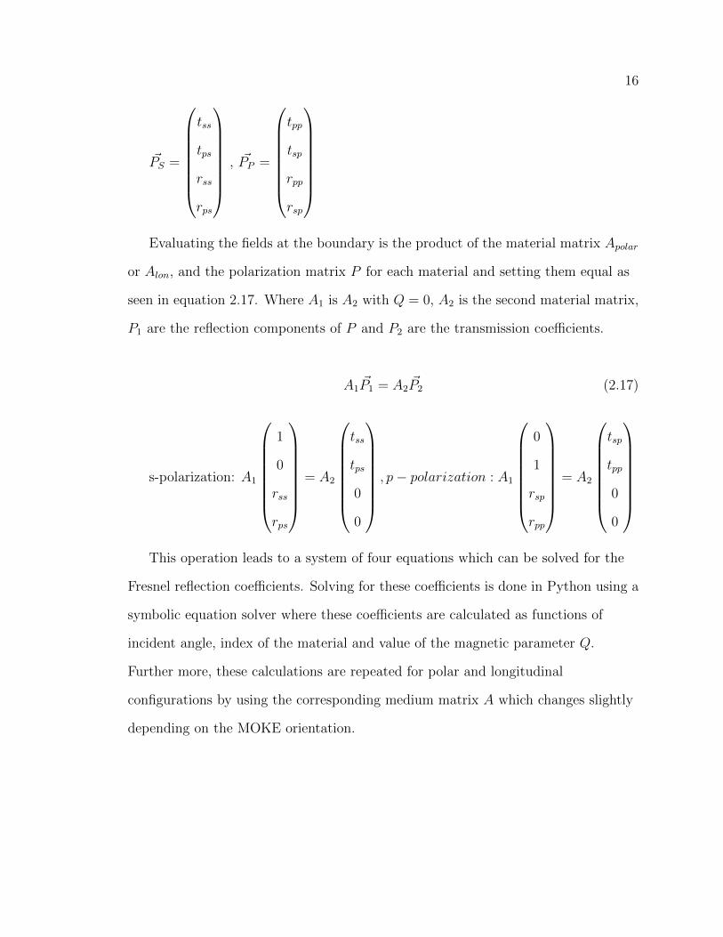
Now the can write ~P for both polarization states as

16

~PS =

tss

tps

rss

rps

, ~PP =

tpp

tsp

rpp

rsp

Evaluating the fields at the boundary is the product of the material matrix Apolar

or Alon, and the polarization matrix P for each material and setting them equal as

seen in equation 2.17. Where A1 is A2 with Q = 0, A2 is the second material matrix,

P1 are the reflection components of P and P2 are the transmission coefficients.

A1~P1 = A2

~P2 (2.17)

s-polarization: A1

1

0

rss

rps

= A2

tss

tps

0

0

, p− polarization : A1

0

1

rsp

rpp

= A2

tsp

tpp

0

0

This operation leads to a system of four equations which can be solved for the

Fresnel reflection coefficients. Solving for these coefficients is done in Python using a

symbolic equation solver where these coefficients are calculated as functions of

incident angle, index of the material and value of the magnetic parameter Q.

Further more, these calculations are repeated for polar and longitudinal

configurations by using the corresponding medium matrix A which changes slightly

depending on the MOKE orientation.

17

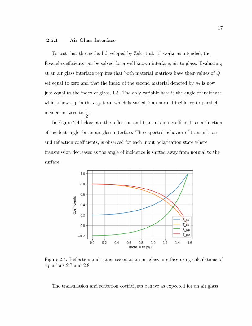
2.5.1 Air Glass Interface

To test that the method developed by Zak et al. [1] works as intended, the

Fresnel coefficients can be solved for a well known interface, air to glass. Evaluating

at an air glass interface requires that both material matrices have their values of Q

set equal to zero and that the index of the second material denoted by n2 is now

just equal to the index of glass, 1.5. The only variable here is the angle of incidence

which shows up in the αz,y term which is varied from normal incidence to parallel

incident or zero toπ

2.

In Figure 2.4 below, are the reflection and transmission coefficients as a function

of incident angle for an air glass interface. The expected behavior of transmission

and reflection coefficients, is observed for each input polarization state where

transmission decreases as the angle of incidence is shifted away from normal to the

surface.

Figure 2.4: Reflection and transmission at an air glass interface using calculations ofequations 2.7 and 2.8

The transmission and reflection coefficients behave as expected for an air glass

18

interface providing validation to the method developed by Zak et. al. The next step

is to now evaluate the interface between air and a magnetically active material.

Solving for the reflection coefficients in this case follows the same general procedure

however the matrix that represents the second medium has non-zero values for the

magnetic parameter Q. This constant serves as the independent variable in the

numerical calculations as increasing the value of Q is analogous to increasing the

strength of the magnetic field. A few other calculations were done in Python as

well, namely varying the angle of incidence and changing the index of the second

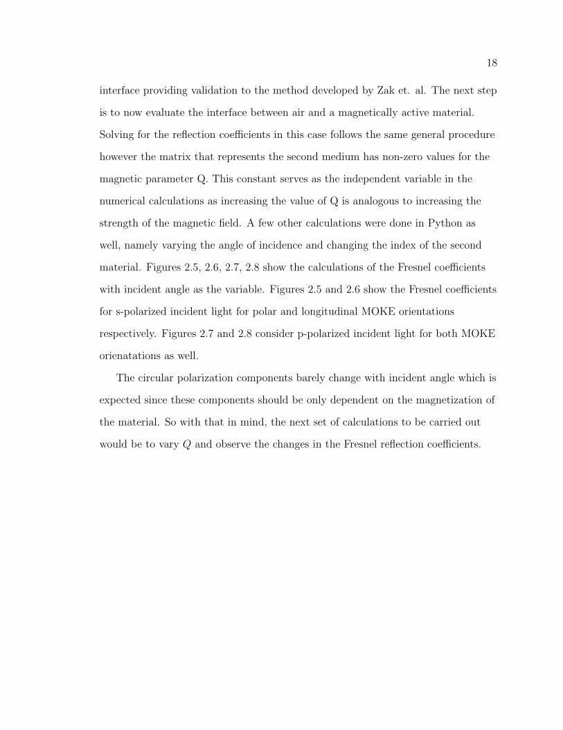
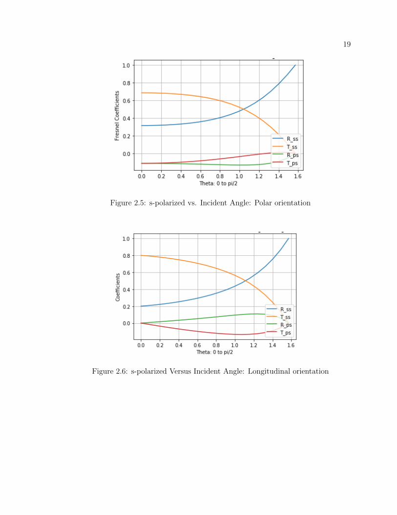
material. Figures 2.5, 2.6, 2.7, 2.8 show the calculations of the Fresnel coefficients

with incident angle as the variable. Figures 2.5 and 2.6 show the Fresnel coefficients

for s-polarized incident light for polar and longitudinal MOKE orientations

respectively. Figures 2.7 and 2.8 consider p-polarized incident light for both MOKE

orienatations as well.

The circular polarization components barely change with incident angle which is

expected since these components should be only dependent on the magnetization of

the material. So with that in mind, the next set of calculations to be carried out

would be to vary Q and observe the changes in the Fresnel reflection coefficients.

19

Figure 2.5: s-polarized vs. Incident Angle: Polar orientation

Figure 2.6: s-polarized Versus Incident Angle: Longitudinal orientation

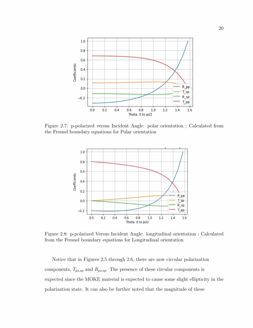
20

Figure 2.7: p-polarized versus Incident Angle: polar orientation ; Calculated fromthe Fresnel boundary equations for Polar orientation

Figure 2.8: p-polarized Versus Incident Angle: longitudinal orientation ; Calculatedfrom the Fresnel boundary equations for Longitudinal orientation

Notice that in Figures 2.5 through 2.6, there are now circular polarization

components, Tps,sp and Rps,sp. The presence of these circular components is

expected since the MOKE material is expected to cause some slight ellipticity in the

polarization state. It can also be further noted that the magnitude of these

21

components are much smaller than the magnitude of the normal polarization states.

The take away from these results is that the numerical model is solving these

boundary conditions and yielding results that are in line with intuition. These

results will be used to create a MOKE Jones matrix which will accurately represent

a MOKE material in the experiment.

2.6 Measuring Phase as Variations in Intensity

Measuring changes in the phase of light is not possible with a photodetector

since photodetectors only measure the intensity of light. Setting up a system of

polarizing optics will allow for changes in polarization to be reflected as changes in

intensity which the photodetector is designed to measure. The simplest method to

reflect changes in polarization as changes in intensity, is by using a polarizer. Then

the intensity of light will follow Malus’ law resulting in changes in intensity as the

polarization angle changes. To improve the performance of the polarizer, quarter

wave plates can convert the slight ellipticity of the polarization state, due to

MOKE, back into linear. This will improve the extinction ratio of the polarizer

meaning less of the wrong polarization will leak through.

2.6.1 Half Wave Plate: Major Axis of Polarization Rotation

Half wave plates are responsible for rotating the major axis of polarization.

Below is a sample calculation demonstrating the effect of a half wave plate on the

polarization of light.

Linearly polarized light at θ =

cos θ

sin θ

22

and the definition of half wave plate =

1 0

0 −1

Evaluting the effect of a half wave plate on the major axis of polarization by

going through the Jones calculation.Eoutx

Eouty

=

1 0

0 −1

cos θ

sin θ

=

cos θ

− sin θ

=

cos−θ

sin−θ

This results tells us that a half wave-plate rotates the axis of polarization from θ

to -θ or rather two times the angle between the angle of the polarization of light and

the fast axis of the wave plate. The purpose of the half wave plate is to rotate the

polarization of light such that it is either parallel (p-polarized) or perpendicular

(s-polarized) relative to the surface of the sample. The incident polarization angle

on the MOKE sample will affect the magnitude of rotation and ellipticity due to

MOKE.

Knowing that the polarization state after the magnetic sample will be some

what elliptical yet the goal is to convert the polarization state back to linear. Using

a quarter wave-plate, elliptical polarization is converted back into linear via

introducing a phase delay to one of the polarization components effectively

“catching it up” with the other component creating linearly polarized light. A

sample calculation has been done to demonstrate this.

2.6.2 Quarter Wave Plate: Circular to Linear Polarization

Conversion

This time, the incident light is going to be circularly polarized, a special case of

elliptical, before passing through the quarter wave plate.

23

Right circular polarization is defined in terms of its Jones vector as:

~RCP =1√2

1

i

A quarter wave plate is defined by its Jones matrix as:

1 0

0 i

Eout

x

Eouty

=

1 0

0 i

1√2

1

i

=1√2

1

−1

The end polarization state has been converted back into linear.

24

CHAPTER 3

NUMERICAL MODEL IN PYTHON

The numerical model developed for this experiment was done in Python. The

goal of the numerical model is to model an optical system capable of measuring the

MOKE rotation and for classifying the performance of the optics that would be used

in said system. The performance of the wave-plates is dependent on the wavelength

of light, the quality of the physical wave-plate itself and whether light is diverging or

converging through the wave plate. Also manufacturing tolerances and misalignment

can affect the performance of optics so an ideal case numerical model is essential.

There are three variables that the numerical model needs to account for, the angle

of the quarter wave-plate and half wave-plate relative to the fast axis and the

strength of the magnetic field. Understanding how the MOKE signal changes with

these variables will produce an ideal case that could be duplicated in a lab setting.

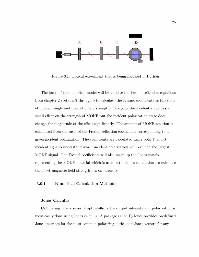
The experimental set up of interest in modeling is seen below in Figure 3.1. The

experiment consists of a A) half wave plate, B) a variable wave plate which is

modeled as a MOKE material in the presence of a magnetic field, C) a quarter

wave-plate and D) a polarizing beam splitting cube. Refer to chapter 2 section 6,

Measuring Phase as Variations in Intensity, for a discussion on why these specific

optics were chosen.

25

Figure 3.1: Optical experiment that is being modeled in Python

The focus of the numerical model will be to solve the Fresnel reflection equations

from chapter 2 sections 3 through 5 to calculate the Fresnel coefficients as functions

of incident angle and magnetic field strength. Changing the incident angle has a

small effect on the strength of MOKE but the incident polarization state does

change the magnitude of the effect significantly. The amount of MOKE rotation is

calculated from the ratio of the Fresnel reflection coefficients corresponding to a

given incident polarization. The coefficients are calculated using both P and S

incident light to understand which incident polarization will result in the largest

MOKE signal. The Fresnel coefficients will also make up the Jones matrix

representing the MOKE material which is used in the Jones calculations to calculate

the effect magnetic field strength has on intensity.

3.0.1 Numerical Calculation Methods

Jones Calculus

Calculating how a series of optics affects the output intensity and polarization is

most easily done using Jones calculus. A package called PyJones provides predefined

Jones matrices for the most common polarizing optics and Jones vectors for any

26

input electric field. Calculating output intensities is done via matrix multiplication

inside a FOR loop that is iterating over the independent variable. Appendix section

A.1 contains the PyJones package definitions for the various optical components.

Symbolic Equation Solving

Solving for the boundary equations across the air to magnetic material interface

was done using the symbolic equation solver in Python. One of the advantages of

using symbolic equations is that the solved equations can be printed out and

checked for potential errors. Segments of code that demonstrate how the Python

program was built in order to solve equations 2.7 through 2.14 can be found in the

Appendix section A.2.

3.1 Results of Python Code

Below are the various graphs generated by the Python code that function either

to calibrate the performance of the optics or to make predictions about the outcome

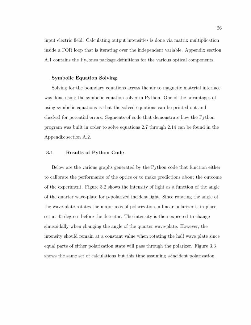
of the experiment. Figure 3.2 shows the intensity of light as a function of the angle

of the quarter wave-plate for p-polarized incident light. Since rotating the angle of

the wave-plate rotates the major axis of polarization, a linear polarizer is in place

set at 45 degrees before the detector. The intensity is then expected to change

sinusoidally when changing the angle of the quarter wave-plate. However, the

intensity should remain at a constant value when rotating the half wave plate since

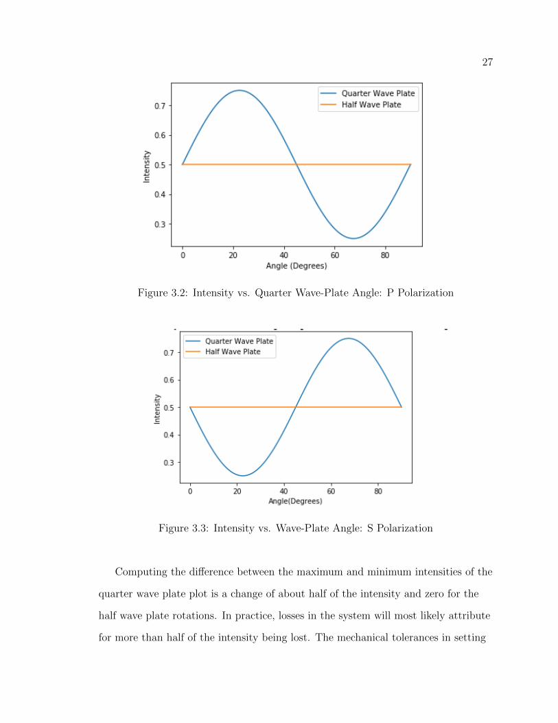
equal parts of either polarization state will pass through the polarizer. Figure 3.3

shows the same set of calculations but this time assuming s-incident polarization.

27

Figure 3.2: Intensity vs. Quarter Wave-Plate Angle: P Polarization

Figure 3.3: Intensity vs. Wave-Plate Angle: S Polarization

Computing the difference between the maximum and minimum intensities of the

quarter wave plate plot is a change of about half of the intensity and zero for the

half wave plate rotations. In practice, losses in the system will most likely attribute

for more than half of the intensity being lost. The mechanical tolerances in setting

28

the angle of the linear polarizer at exactly 45 degrees means that the extinction

ratio of the polarizer will not be ideal.

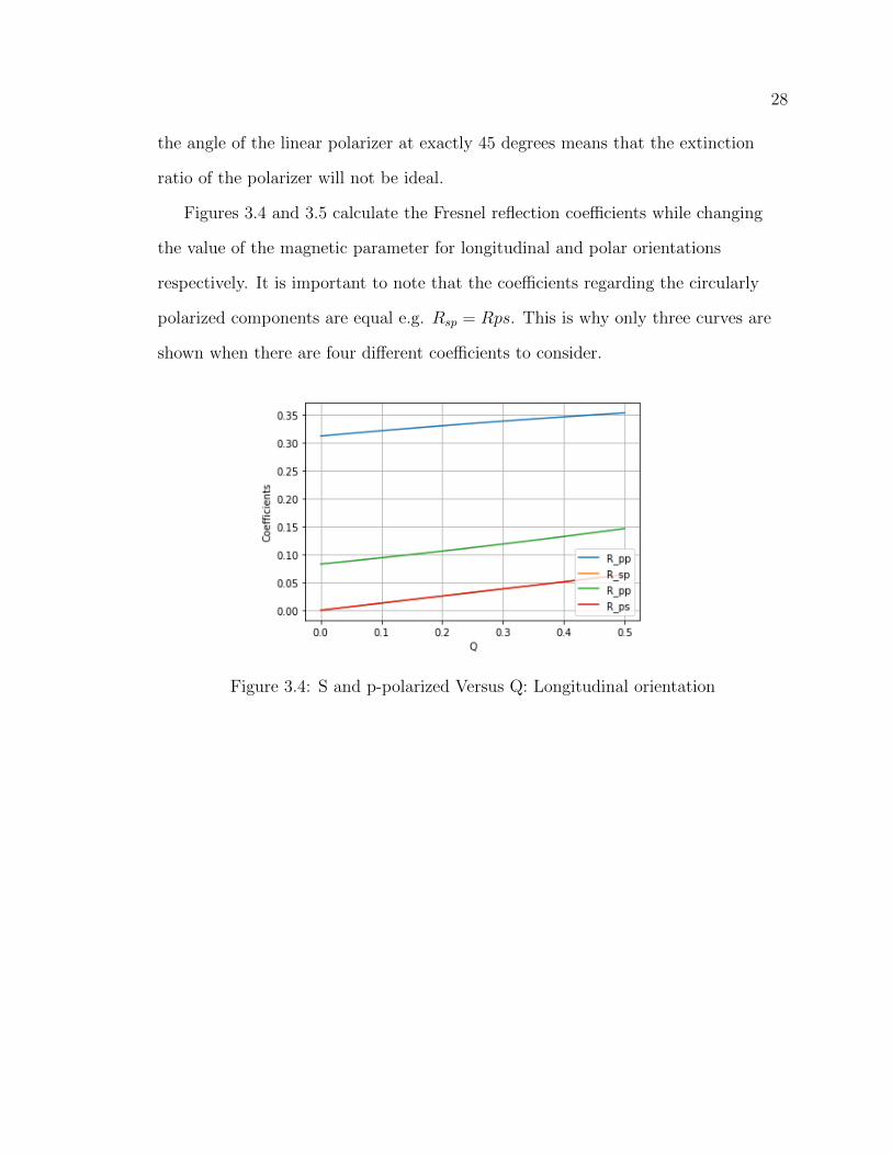
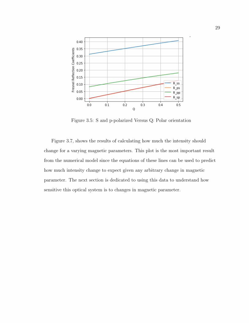
Figures 3.4 and 3.5 calculate the Fresnel reflection coefficients while changing

the value of the magnetic parameter for longitudinal and polar orientations

respectively. It is important to note that the coefficients regarding the circularly

polarized components are equal e.g. Rsp = Rps. This is why only three curves are

shown when there are four different coefficients to consider.

Figure 3.4: S and p-polarized Versus Q: Longitudinal orientation

29

Figure 3.5: S and p-polarized Versus Q: Polar orientation

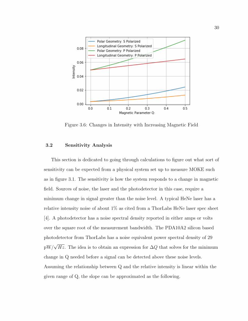
Figure 3.7, shows the results of calculating how much the intensity should

change for a varying magnetic parameters. This plot is the most important result

from the numerical model since the equations of these lines can be used to predict

how much intensity change to expect given any arbitrary change in magnetic

parameter. The next section is dedicated to using this data to understand how

sensitive this optical system is to changes in magnetic parameter.

30

Figure 3.6: Changes in Intensity with Increasing Magnetic Field

3.2 Sensitivity Analysis

This section is dedicated to going through calculations to figure out what sort of

sensitivity can be expected from a physical system set up to measure MOKE such

as in figure 3.1. The sensitivity is how the system responds to a change in magnetic

field. Sources of noise, the laser and the photodetector in this case, require a

minimum change in signal greater than the noise level. A typical HeNe laser has a

relative intensity noise of about 1% as cited from a ThorLabs HeNe laser spec sheet

[4]. A photodetector has a noise spectral density reported in either amps or volts

over the square root of the measurement bandwidth. The PDA10A2 silicon based

photodetector from ThorLabs has a noise equivalent power spectral density of 29

pW/√Hz. The idea is to obtain an expression for ∆Q that solves for the minimum

change in Q needed before a signal can be detected above these noise levels.

Assuming the relationship between Q and the relative intensity is linear within the

given range of Q, the slope can be approximated as the following.

31

M =∆V O

Pol

∆Qmodel

(3.1)

Where ∆V OPol is the range of relative intensity values from the Python model for

a given MOKE orientation, O, and incident polarization, Pol. Writing a general

equation for each of the intensity versus Q lines as

∆Vm = M∆Q (3.2)

Solving for ∆Q based on an relative intensity change is then calculated as

∆Q = M−1∆Vm (3.3)

Where ∆Vm is the change in relative intensity value as measured by a

photodetector.

The other condition required is that ∆Vm > ∆Vmin where ∆Vmin is the smallest

detectable power. For example, a HeNe laser from ThorLabs [4], has a amplitude

stability of 1% meaning that, for a direct measurement, the change in intensity due

to MOKE needs to be greater than 1% of the laser power. Using the slope of each

line, a minimum change in ∆Q is obtained that is required to produce a signal

above the relative amplitude noise of the laser for a given MOKE orientation and

incident polarization.

∆QPolarS = .24

∆QPolarP = .12

∆QLONS = .31

∆QLONP = .54

From these results, polar orientation and p-polarization incident light has the

32

smallest value for change Q which indicates the highest sensitivity in that

configuration. However, there is not just laser noise but also noise from the

photodetector that needs to considered for an accurate value for ∆Q to be obtained.

A PDA10A2 ThorLabs silicon based photodetector has a typical noise equivalent

power spectral density of 29.2 pW/√Hz meaning it has an average noise level of

29.2 pW[3] in a one second measurement. Calculating the cutoff frequency beyond

which the measurement is limited by detector noise by solving the follow equation

for ∆f .

Noise = 29.2pW/√Hz ×

√∆f (3.4)

∆f =Noise

29.2pW/√Hz

(3.5)

Solving for ∆f using 1% of the 285 mW output of the laser as the noise returns

96 MHz for the cutoff frequency.

With a photodetector noise level of 29.2 pW, the required change in Q to

produce a signal above that limit is calculated using equation 3.3. The results of

that calculation are seen below for both polar and longitudinal orientations and s

and p-polarization.

∆QPolarS = 5.9× 10−11

∆QPolarP = 2.9× 10−11

∆QLONS = 7.8× 10−11

∆QLONP = 1.3× 10−10

The sensitivity of the system drastically improves if the only source of noise is

from the photodetector. In the next section, there will be a discussion on how to

improve the sensitivity of the system using experimental techniques.

33

3.3 Sensitivity Improvements

This section is dedicated to looking at various experimental techniques that

could be used in order to increase the sensitivity of an optical system to isolate the

polarization rotation due to MOKE.

3.3.1 Balanced Detection

The method of balanced detection focuses on detecting the difference between

two signals. In the case of this experiment, the two signals that could be measured

are the two beams coming from the polarizing beam splitting cube. If the incident

polarization on the cube is set to 45 degrees, then equal amount of intensity will

travel down each path hence the “balanced” part of the detection. If there is a

non-zero change in the major axis of polarization, then there will not be equal

intensities in each beam and a non-zero signal in the difference in intensity of the

beams will be obtained. Doing a balance detection also doubles the amount of signal

that would be detected and eliminates the noise due to the laser. One beam coming

out of the cube will contain both the background noise plus the MOKE signal and

the other beam will have the background noise minus the MOKE signal. So taking

the difference between these two beams would result in doubling the MOKE signal

measured and suppressing any laser noise. However, the implicit assumption here is

that the polarizing beam splitting cube perfectly splits the polarization components.

In practice, polarizing beam splitting cubes have extinction ratios of around 30 dB

meaning that one part in a thousand of the wrong polarization leaks through. So in

reality, laser noise is not completely eliminated but reduced by three orders of

magnitude which still drastically improves the sensitivity.

34

3.3.2 Modulated Detection

Another technique that can be used to increase sensitivity involves modulating

the magnetic field with a current source driven by a function generator and using a

lock-in amplifier to recover the MOKE signal. Modulating the current at a

frequency on the order of hertz will vary the magnetic field strength over time which

will also vary the amount of the polarization rotation at the same frequency. Doing

this also moves the MOKE signal into a frequency where noise could be lower. For

instance the low frequency noise of background room lights or 1/f might motivate

someone to shift the MOKE signal into a different frequency channel. A lock-in

amplifier can be used to recover the MOKE signal after it has been frequency

shifted. The reference for the lock-in amplifier will be the frequency of the current

modulator. In the absence of low frequency noise, modulation detection does not

present any significant advantages when compared to balanced detection.

35

CHAPTER 4

FUTURE WORK: EXPERIMENT

This chapter is dedicated to designing an optical system that would be capable

of measuring the polarization rotation due to MOKE. The experimental work that

is needed for this thesis project was intended to be done as apart of this project.

However, the COVID-19 pandemic forced San Jose State University to close and I

was unable to finish the experimental side of the work. The rest of the experiment

remains as future work.

4.1 Polarization Measurement System

The optical system that allows for polarization measurement utilizes the effects

of wave-plates on the polarization of light to measure the changes in intensity due to

MOKE. To control the incident polarization on the sample, a half wave plate is

placed right after the laser source. This half-wave plate will then rotate the

polarization of the laser by two times the angle between the incident polarization

and the optical axis of the wave plate. The magnitude of MOKE is dependent upon

the incident polarization of light on the sample. The effect is maximized when the

light is p-polarized for the longitudinal MOKE orientation. The next element would

be the MOKE sample which typically is a thin film of nickle. Surrounding the

sample, are a pair of Helmholtz coils which apply a field parallel to the surface of

the sample which activates the magneto optic properties of the material. The next

optical element is a quarter wave-plate to correct the slight ellipticity in the

polarization of the light coming from the sample and return it to linearly polarized

36

light. The angle of the linearly polarized light will depend on the amount of

polarization rotation due to MOKE. The polarizer is set to 45 degrees which makes

the system the most sensitive to changes in intensity.

4.2 Interpreting Results

Without an explicit expression for the magnetic parameter as a function of

magnetic field strength, Q(B), there needs to be a way to interpret the

measurement performed in the lab. The numerical model in Python provides a

model of intensity change versus the magnetic parameter, Q, but experimentally, it

needs to be calibrated against a known magnetic field. Calibrating experimental

data can be done by measuring the change in intensity at various magnetic field

strengths. A pair of Helmholtz coils can generate a uniform field around the sample

at various magnetic field strengths using a current source. Measuring the change in

intensity at a few points and fitting the data will generate an expression for

intensity as a function of magnetic field strength allowing for any arbitrary change

in intensity to be related to a specific magnetic field strength.

4.3 Imaging System Design

The next task in this project is to image the surface of the sample onto a CCD

sensor. The imaging system could be a basic two lens, 4F system that captures the

nearly collimated light from the sample and then fully collimates the light before

passing through the optics. There are a few constraints of this system that need to

be considered when choosing the lens sizes for the imaging system. The surface of

the samples range from fairly smooth and uniform to rough which means that in

either case, light will scatter from the surface reducing the overall intensity

37

measured. This means the first lens in the imaging system needs to be as large as

possible. The lenses that are used are 1 inch in diameter and will be sufficient for

capturing enough light. Assuming a lens has been chosen to collect the most light,

the light then needs to be collimated before passing through the rest of the optical

system. The one inch diameter lenses will collimate the light at a diameter that is

smaller than the diameter of the wave-plates so only two lenses are needed in order

to image the sample onto the sensor.

When building an imaging system, evaluating the conditions under which

vignetting will occur, provides constraints on the size of the optics that can be

chosen. Checking for vignetting is done by creating a ray tracing diagram that

traces rays coming from extreme points on the object. Considering a point on the

object far from the optical axis, will show whether or not those rays will make it

through all of the lenses. The chief ray is the ray coming from the most off center

point on the object and passes through the first lens. It continues on and intersects

the vertical plane passing through the second lens. If the point of intersection

between the ray and the vertical plane at the second lens is larger than the diameter

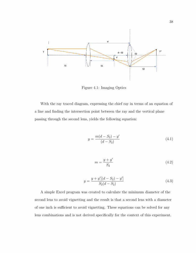
of the second lens, vignetting will occur. Below is the ray traced diagram, Figure

4.1, showing the chief ray coming from the object as well as a secondary ray to

locate the intermediate and final image.

38

Figure 4.1: Imaging Optics

With the ray traced diagram, expressing the chief ray in terms of an equation of

a line and finding the intersection point between the ray and the vertical plane

passing through the second lens, yields the following equation:

y =m(d− S2)− y′

(d− S2)(4.1)

m =y + y′

S2

(4.2)

y =y + y′[(d− S2)− y′]

S2(d− S2)(4.3)

A simple Excel program was created to calculate the minimum diameter of the

second lens to avoid vignetting and the result is that a second lens with a diameter

of one inch is sufficient to avoid vignetting. These equations can be solved for any

lens combinations and is not derived specifically for the context of this experiment.

39

CHAPTER 5

CONCLUSION

The results of this project have laid out the foundation to build a physical

system in order to measure MOKE and a few techniques in order to improve the

sensitivity of the experiment. The relationship between the magnetic parameter, Q,

and change in intensity has been modeled in Python. The experimental calibration

to determine the relationship between Q and B which is necessary to interpret the

results of the model in terms of magnetic field, remains future work. I was able to

build an optical system that made use of balanced detection but could not acquire

experimental data with SJSU closed due to the COVID-19 outbreak. The data that

would be taken in the lab would determine the relationship between magnetic field

strength and intensity change. This data can then be used along with the numerical

model data to calibrate the experiment and determine the relationship between

magnetic field, B, and the magnetic parameter, Q. The take away from the results

of this paper are that the best sensitivity can be achieved with a polar MOKE

orientation and using P incident polarized light. The model in Python also predicts

that the change in relative intensity will be approximately 1 - 2%, depending on

orientation and polarization, as calculated as the difference in the normalized

intensity over the range of Q seen in Figure 3.7. So making a balanced detection

measurement, in a polar orientation with P incident light sets up the most sensitive

configuration as predicted by this analysis.

40

APPENDIX A

APPENDIX

A.1 PyJones

# Imported Optics from PyJones

from pyjones.opticalelements import Polarizer

from pyjones.opticalelements import HalfWavePlate

from pyjones.opticalelements import PolarizerVertical

from pyjones.opticalelements import QuarterWavePlate

from pyjones.opticalelements import JonesMatrix

#Imported Input Polarization States from PyJones

from pyjones.polarizations import LinearHorizontal

from pyjones.polarizations import LinearVertical

from pyjones.polarizations import CircularRight

from pyjones.polarizations import CircularLeft

Polarization States:

print LinearVertical()

out: JonesVector([0j, (1+0j)])

A quick note here, the printout of 1x2 matrices in Python is seen as a 2x1 instead

since it has to print out the information on a single line.

print QuarterWavePlate(0). # zero denotes fast axis aligned

out: JonesMatrix(0.7+0j), 0j],[0j, (0+0.7j)

41

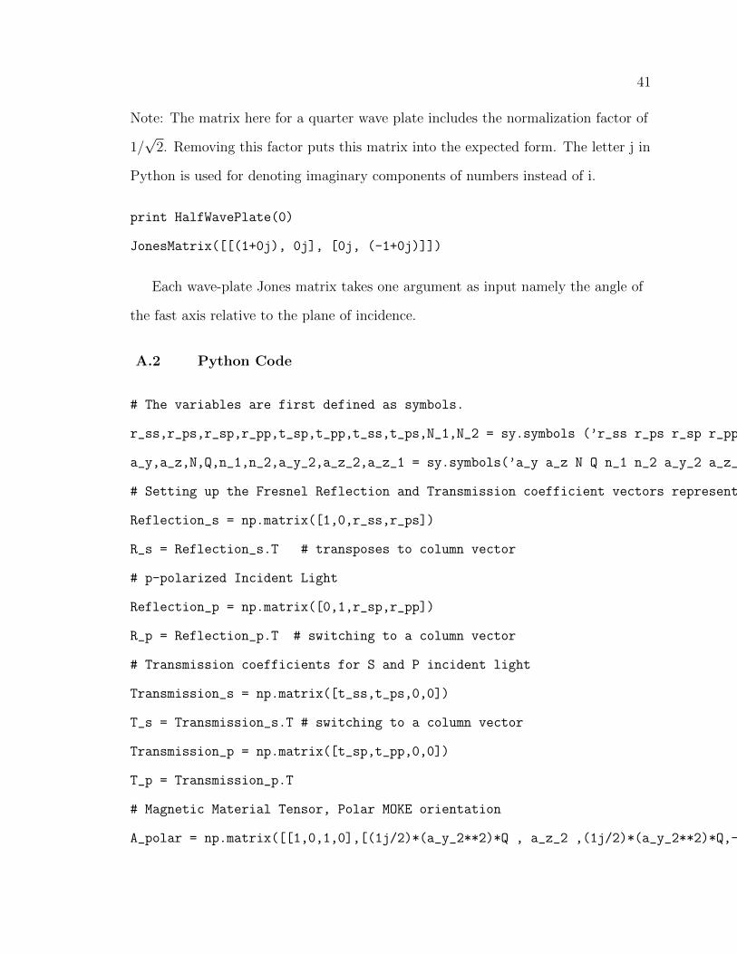
Note: The matrix here for a quarter wave plate includes the normalization factor of

1/√

2. Removing this factor puts this matrix into the expected form. The letter j in

Python is used for denoting imaginary components of numbers instead of i.

print HalfWavePlate(0)

JonesMatrix([[(1+0j), 0j], [0j, (-1+0j)]])

Each wave-plate Jones matrix takes one argument as input namely the angle of

the fast axis relative to the plane of incidence.

A.2 Python Code

# The variables are first defined as symbols.

r_ss,r_ps,r_sp,r_pp,t_sp,t_pp,t_ss,t_ps,N_1,N_2 = sy.symbols (’r_ss r_ps r_sp r_pp t_sp t_pp t_ss t_ps N_1 N_2’)

a_y,a_z,N,Q,n_1,n_2,a_y_2,a_z_2,a_z_1 = sy.symbols(’a_y a_z N Q n_1 n_2 a_y_2 a_z_2 a_z_1’)

# Setting up the Fresnel Reflection and Transmission coefficient vectors representing the fields.

Reflection_s = np.matrix([1,0,r_ss,r_ps])

R_s = Reflection_s.T # transposes to column vector

# p-polarized Incident Light

Reflection_p = np.matrix([0,1,r_sp,r_pp])

R_p = Reflection_p.T # switching to a column vector

# Transmission coefficients for S and P incident light

Transmission_s = np.matrix([t_ss,t_ps,0,0])

T_s = Transmission_s.T # switching to a column vector

Transmission_p = np.matrix([t_sp,t_pp,0,0])

T_p = Transmission_p.T

# Magnetic Material Tensor, Polar MOKE orientation

A_polar = np.matrix([[1,0,1,0],[(1j/2)*(a_y_2**2)*Q , a_z_2 ,(1j/2)*(a_y_2**2)*Q,-a_z_2],[(1j/2)*(a_z_2)*Q*N, -N ,-(1j/2)*(a_z_2)*Q*N, -N] ,[a_z_2*N, (1j/2)*Q*N, -a_z_2*N, (1j/2)*Q*N]])

42

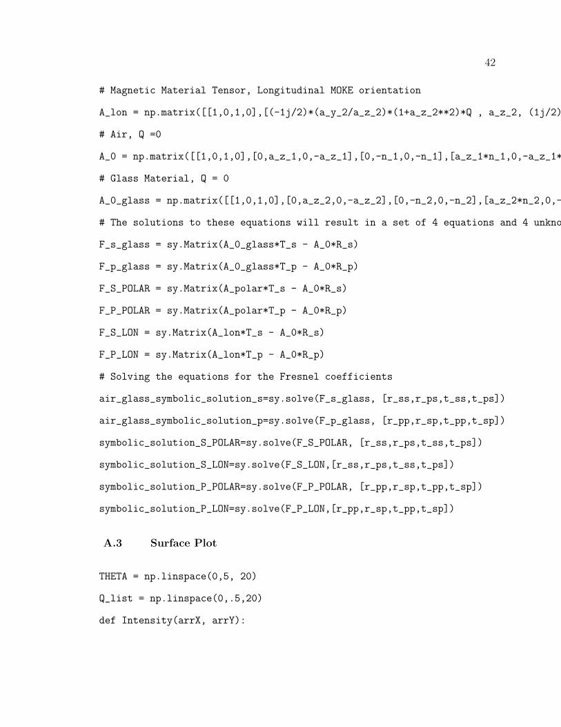
# Magnetic Material Tensor, Longitudinal MOKE orientation

A_lon = np.matrix([[1,0,1,0],[(-1j/2)*(a_y_2/a_z_2)*(1+a_z_2**2)*Q , a_z_2, (1j/2)*(a_y_2/a_z_2)*(1+a_z_2**2)*Q, -a_z_2],[(1j/2)*a_y_2*Q*N,-N,(1j/2)*a_y_2*Q*N,-N],[a_z_2*N,(1j/2)*(a_y_2/a_z_2)*Q*N,-a_z_2*N,-(1j/2)*(a_y_2/a_z_2)*Q*N]]) # non magnetic material Q = 0

# Air, Q =0

A_0 = np.matrix([[1,0,1,0],[0,a_z_1,0,-a_z_1],[0,-n_1,0,-n_1],[a_z_1*n_1,0,-a_z_1*n_1,0]])

# Glass Material, Q = 0

A_0_glass = np.matrix([[1,0,1,0],[0,a_z_2,0,-a_z_2],[0,-n_2,0,-n_2],[a_z_2*n_2,0,-a_z_2*n_2,0]])

# The solutions to these equations will result in a set of 4 equations and 4 unknowns in matrix form.

F_s_glass = sy.Matrix(A_0_glass*T_s - A_0*R_s)

F_p_glass = sy.Matrix(A_0_glass*T_p - A_0*R_p)

F_S_POLAR = sy.Matrix(A_polar*T_s - A_0*R_s)

F_P_POLAR = sy.Matrix(A_polar*T_p - A_0*R_p)

F_S_LON = sy.Matrix(A_lon*T_s - A_0*R_s)

F_P_LON = sy.Matrix(A_lon*T_p - A_0*R_p)

# Solving the equations for the Fresnel coefficients

air_glass_symbolic_solution_s=sy.solve(F_s_glass, [r_ss,r_ps,t_ss,t_ps])

air_glass_symbolic_solution_p=sy.solve(F_p_glass, [r_pp,r_sp,t_pp,t_sp])

symbolic_solution_S_POLAR=sy.solve(F_S_POLAR, [r_ss,r_ps,t_ss,t_ps])

symbolic_solution_S_LON=sy.solve(F_S_LON,[r_ss,r_ps,t_ss,t_ps])

symbolic_solution_P_POLAR=sy.solve(F_P_POLAR, [r_pp,r_sp,t_pp,t_sp])

symbolic_solution_P_LON=sy.solve(F_P_LON,[r_pp,r_sp,t_pp,t_sp])

A.3 Surface Plot

THETA = np.linspace(0,5, 20)

Q_list = np.linspace(0,.5,20)

def Intensity(arrX, arrY):

43

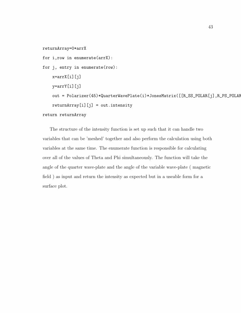
returnArray=0*arrX

for i,row in enumerate(arrX):

for j, entry in enumerate(row):

x=arrX[i][j]

y=arrY[i][j]

out = Polarizer(45)*QuarterWavePlate(i)*JonesMatrix([[R_SS_POLAR[j],R_PS_POLAR[j]],[R_SP_POLAR[j],R_PP_POLAR[j]]])*HalfWavePlate(0)*input_polarization_1

returnArray[i][j] = out.intensity

return returnArray

The structure of the intensity function is set up such that it can handle two

variables that can be ’meshed’ together and also perform the calculation using both

variables at the same time. The enumerate function is responsible for calculating

over all of the values of Theta and Phi simultaneously. The function will take the

angle of the quarter wave-plate and the angle of the variable wave-plate ( magnetic

field ) as input and return the intensity as expected but in a useable form for a

surface plot.

44

BIBLIOGRAPHY

[1] Zak, J., et al. “Universal Approach to Magneto-Optics.”Journal of Magnetismand Magnetic Materials, vol. 89, no. 1-2, 5 Mar. 1990, pp. 107–123.,doi:10.1016/0304-8853(90)90713-z.

[2] Lewis, E. Percival, et al. The Effects of a Magnetic Field on Radiation ;Memoirs. American Book Co., 1900.

[3] “Free-Space Biased Detectors.” THORLABS, Thor Labs,www.thorlabs.com/newgrouppage9.cfm?objectgroupid=1295.

[4] “Stabilized Red HeNe Laser.” THORLABS, THORLABS,www.thorlabs.com/newgrouppage9.cfm?objectgroupid=5281.

[5] Jackson, John David. Classical Electrodynamics. N.p.: Wiley, 2016. Print.