Embed Size (px)
Citation preview
1
1
Microprocessor architecture and instruction execution
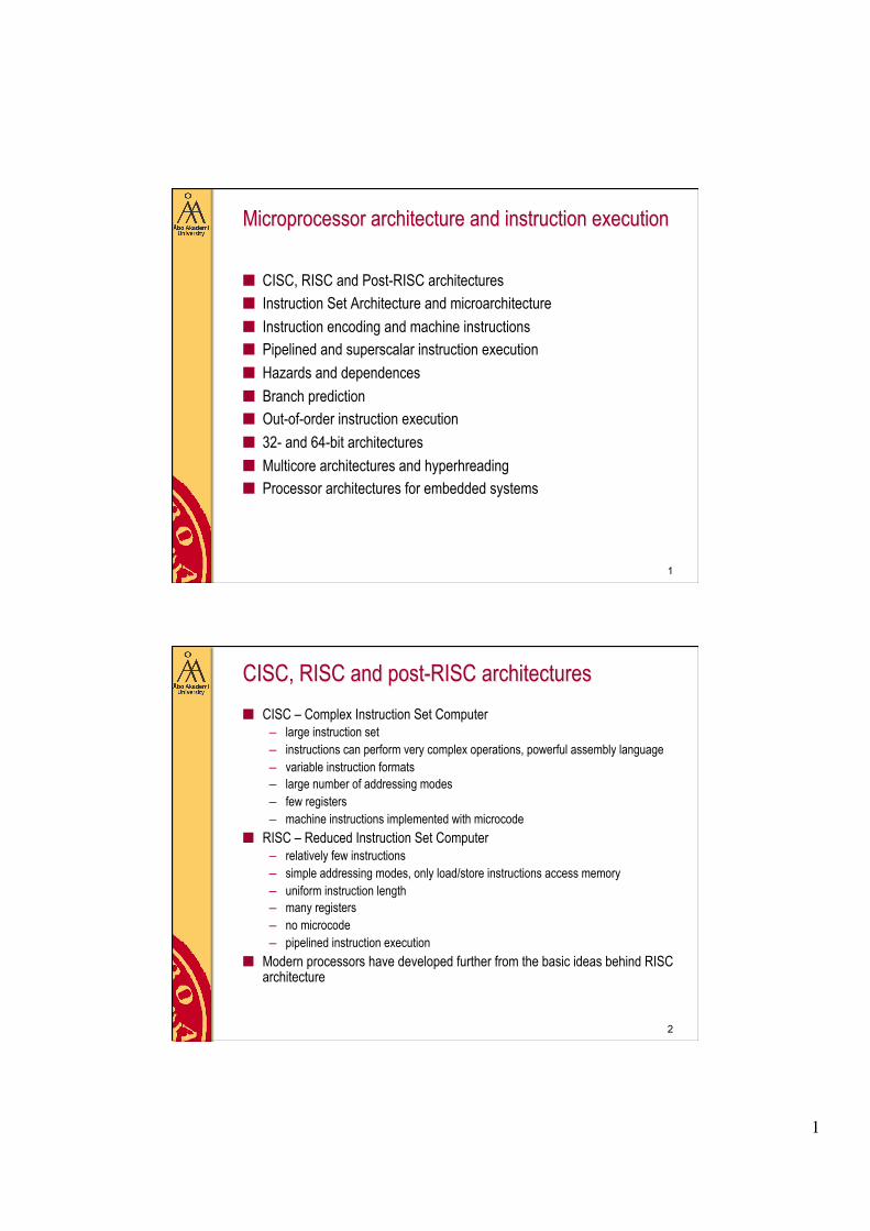
■ CISC, RISC and Post-RISC architectures ■ Instruction Set Architecture and microarchitecture ■ Instruction encoding and machine instructions ■ Pipelined and superscalar instruction execution ■ Hazards and dependences ■ Branch prediction ■ Out-of-order instruction execution ■ 32- and 64-bit architectures ■ Multicore architectures and hyperhreading ■ Processor architectures for embedded systems
2
CISC, RISC and post-RISC architectures ■ CISC – Complex Instruction Set Computer
– large instruction set – instructions can perform very complex operations, powerful assembly language – variable instruction formats – large number of addressing modes – few registers – machine instructions implemented with microcode
■ RISC – Reduced Instruction Set Computer – relatively few instructions – simple addressing modes, only load/store instructions access memory – uniform instruction length – many registers – no microcode – pipelined instruction execution
■ Modern processors have developed further from the basic ideas behind RISC architecture
2
3
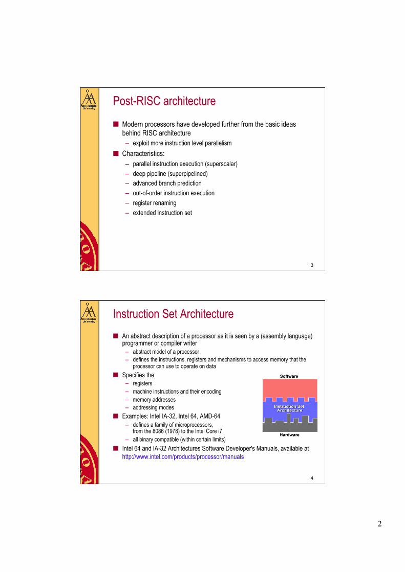
Post-RISC architecture
■ Modern processors have developed further from the basic ideas behind RISC architecture – exploit more instruction level parallelism
■ Characteristics: – parallel instruction execution (superscalar) – deep pipeline (superpipelined) – advanced branch prediction – out-of-order instruction execution – register renaming – extended instruction set
4
Instruction Set Architecture ■ An abstract description of a processor as it is seen by a (assembly language)
programmer or compiler writer – abstract model of a processor – defines the instructions, registers and mechanisms to access memory that the
processor can use to operate on data ■ Specifies the
– registers – machine instructions and their encoding – memory addresses – addressing modes
■ Examples: Intel IA-32, Intel 64, AMD-64 – defines a family of microprocessors,
from the 8086 (1978) to the Intel Core i7 – all binary compatible (within certain limits)
■ Intel 64 and IA-32 Architectures Software Developer's Manuals, available at http://www.intel.com/products/processor/manuals
3
5
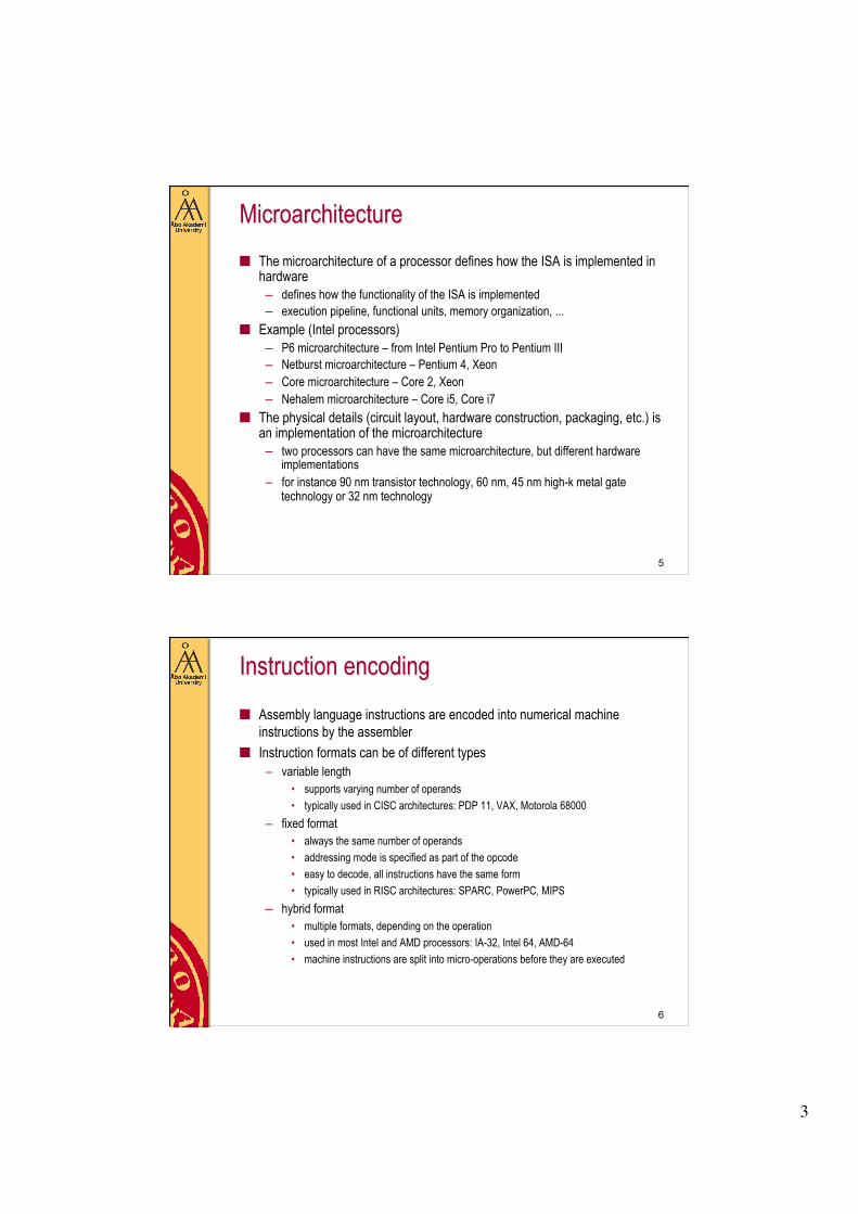
Microarchitecture ■ The microarchitecture of a processor defines how the ISA is implemented in
hardware – defines how the functionality of the ISA is implemented – execution pipeline, functional units, memory organization, ...
■ Example (Intel processors) – P6 microarchitecture – from Intel Pentium Pro to Pentium III – Netburst microarchitecture – Pentium 4, Xeon – Core microarchitecture – Core 2, Xeon – Nehalem microarchitecture – Core i5, Core i7
■ The physical details (circuit layout, hardware construction, packaging, etc.) is an implementation of the microarchitecture – two processors can have the same microarchitecture, but different hardware
implementations – for instance 90 nm transistor technology, 60 nm, 45 nm high-k metal gate
technology or 32 nm technology
6
Instruction encoding ■ Assembly language instructions are encoded into numerical machine
instructions by the assembler ■ Instruction formats can be of different types
– variable length • supports varying number of operands • typically used in CISC architectures: PDP 11, VAX, Motorola 68000
– fixed format • always the same number of operands • addressing mode is specified as part of the opcode • easy to decode, all instructions have the same form • typically used in RISC architectures: SPARC, PowerPC, MIPS
– hybrid format • multiple formats, depending on the operation • used in most Intel and AMD processors: IA-32, Intel 64, AMD-64 • machine instructions are split into micro-operations before they are executed
4
7
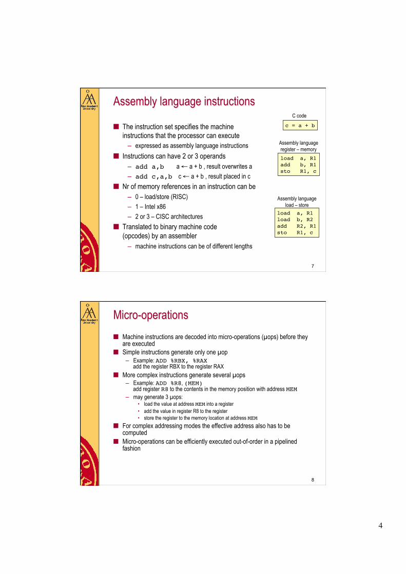
Assembly language instructions
■ The instruction set specifies the machine instructions that the processor can execute
– expressed as assembly language instructions ■ Instructions can have 2 or 3 operands
– add a,b a ← a + b , result overwrites a – add c,a,b c ← a + b , result placed in c
■ Nr of memory references in an instruction can be – 0 – load/store (RISC) – 1 – Intel x86 – 2 or 3 – CISC architectures
■ Translated to binary machine code (opcodes) by an assembler
– machine instructions can be of different lengths
c = a + b!
C code
load a, R1!add b, R1!sto R1, c!
Assembly language register – memory
load a, R1!load b, R2!add R2, R1!sto R1, c!
Assembly language load – store
8
Micro-operations ■ Machine instructions are decoded into micro-operations (µops) before they
are executed ■ Simple instructions generate only one µop
– Example: ADD %RBX, %RAX add the register RBX to the register RAX
■ More complex instructions generate several µops – Example: ADD %R8, (MEM)
add register R8 to the contents in the memory position with address MEM – may generate 3 µops:
• load the value at address MEM into a register • add the value in register R8 to the register • store the register to the memory location at address MEM
■ For complex addressing modes the effective address also has to be computed
■ Micro-operations can be efficiently executed out-of-order in a pipelined fashion
5
9
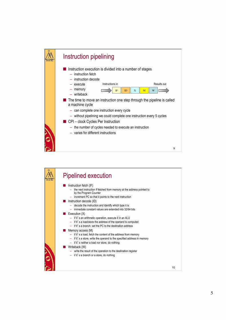
Instruction pipelining ■ Instruction execution is divided into a number of stages
– instruction fetch – instruction decode – execute – memory – writeback
■ The time to move an instruction one step through the pipeline is called a machine cycle – can complete one instruction every cycle – without pipelining we could complete one instruction every 5 cycles
■ CPI – clock Cycles Per Instruction – the number of cycles needed to execute an instruction – varies for different instructions
IF ID M W
Instructions in Results out
X
10
Pipelined execution ■ Instruction fetch (IF)
– the next instruction if fetched from memory at the address pointed to by the Program Counter
– increment PC so that it points to the next instruction ■ Instruction decode (ID)
– decode the instruction and identify which type it is – immediate constant values are extended into 32/64 bits
■ Execution (X) – if it’s an arithmetic operation, execute it in an ALU – if it’s a load/store the address of the operand is computed – if it’s a branch, set the PC to the destination address
■ Memory access (M) – if it’s a load, fetch the content of the address from memory – if it’s a store, write the operand to the specified address in memory – if it’s neither a load nor store, do nothing
■ Writeback (W) – write the result of the operation to the destination register – if it’s a branch or a store, do nothing
6
11
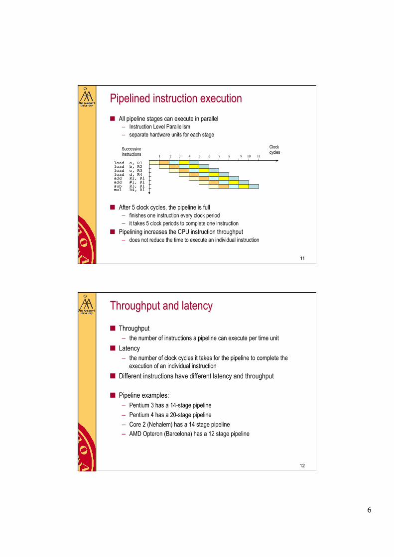
Pipelined instruction execution ■ All pipeline stages can execute in parallel
– Instruction Level Parallelism – separate hardware units for each stage
■ After 5 clock cycles, the pipeline is full – finishes one instruction every clock period – it takes 5 clock periods to complete one instruction
■ Pipelining increases the CPU instruction throughput – does not reduce the time to execute an individual instruction
Successive instructions
Clock cycles
1 2 3 4 5 6 7 8 9 10 11
load a, R1!load b, R2!load c, R3!load d, R4!add R2, R1!add #1, R1!sub R3, R1!mul R4, R1!
12
Throughput and latency
■ Throughput – the number of instructions a pipeline can execute per time unit
■ Latency – the number of clock cycles it takes for the pipeline to complete the
execution of an individual instruction ■ Different instructions have different latency and throughput
■ Pipeline examples:
– Pentium 3 has a 14-stage pipeline – Pentium 4 has a 20-stage pipeline – Core 2 (Nehalem) has a 14 stage pipeline – AMD Opteron (Barcelona) has a 12 stage pipeline
7
13
Superscalar architecture
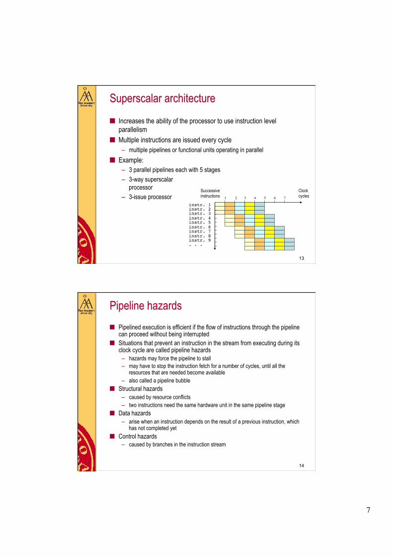
■ Increases the ability of the processor to use instruction level parallelism
■ Multiple instructions are issued every cycle – multiple pipelines or functional units operating in parallel
■ Example: – 3 parallel pipelines each with 5 stages – 3-way superscalar
processor – 3-issue processor
Successive instructions
Clock cycles 1 2 3 4 5 6 7
instr. 1!instr. 2!instr. 3!instr. 4!instr. 5!instr. 6!instr. 7!instr. 8!instr. 9!. . .!
14
Pipeline hazards ■ Pipelined execution is efficient if the flow of instructions through the pipeline
can proceed without being interrupted ■ Situations that prevent an instruction in the stream from executing during its
clock cycle are called pipeline hazards – hazards may force the pipeline to stall – may have to stop the instruction fetch for a number of cycles, until all the
resources that are needed become available – also called a pipeline bubble
■ Structural hazards – caused by resource conflicts – two instructions need the same hardware unit in the same pipeline stage
■ Data hazards – arise when an instruction depends on the result of a previous instruction, which
has not completed yet ■ Control hazards
– caused by branches in the instruction stream
8
15
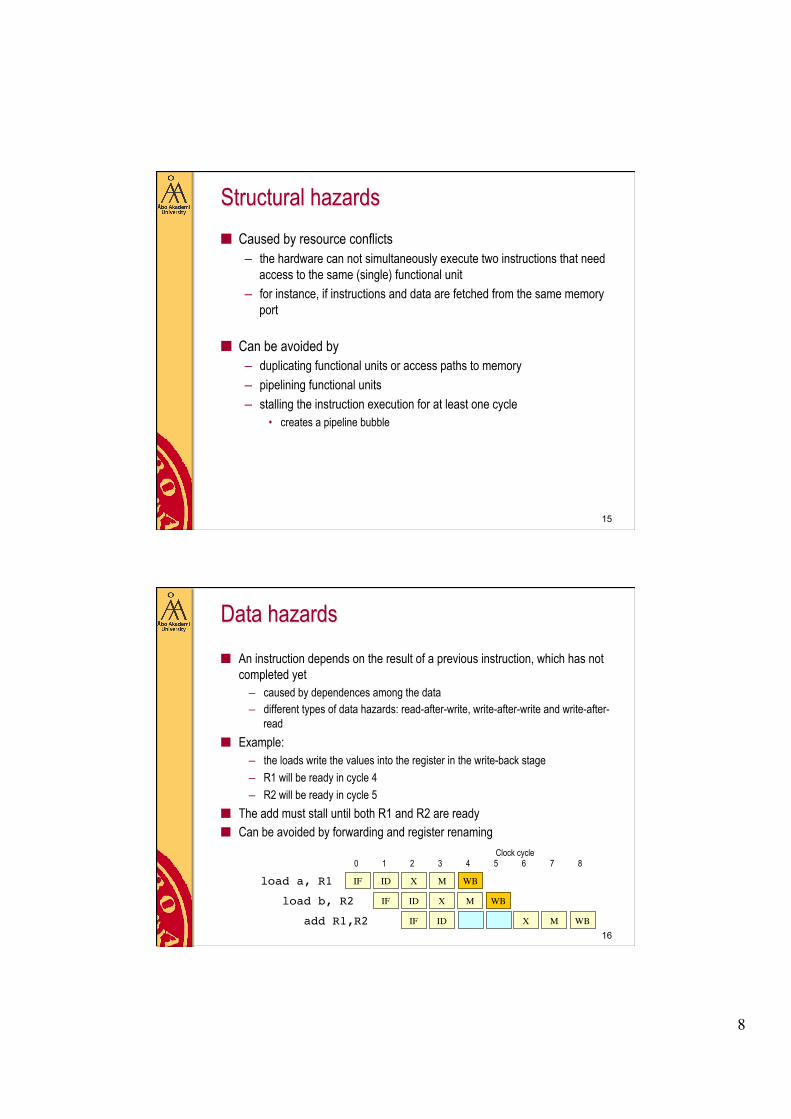
Structural hazards ■ Caused by resource conflicts
– the hardware can not simultaneously execute two instructions that need access to the same (single) functional unit
– for instance, if instructions and data are fetched from the same memory port
■ Can be avoided by – duplicating functional units or access paths to memory – pipelining functional units – stalling the instruction execution for at least one cycle
• creates a pipeline bubble
16
Data hazards ■ An instruction depends on the result of a previous instruction, which has not
completed yet – caused by dependences among the data – different types of data hazards: read-after-write, write-after-write and write-after-
read ■ Example:
– the loads write the values into the register in the write-back stage – R1 will be ready in cycle 4 – R2 will be ready in cycle 5
■ The add must stall until both R1 and R2 are ready ■ Can be avoided by forwarding and register renaming
IF ID M WB X
IF ID M WB X
IF ID M WB X
Clock cycle 0 1 2 3 4 5 6
load a, R1!
load b, R2!
add R1,R2!
7 8
9
17
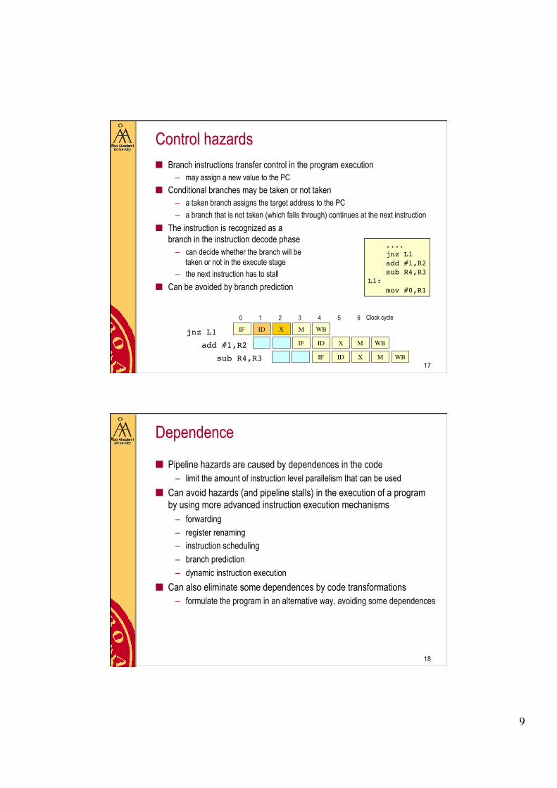
Control hazards ■ Branch instructions transfer control in the program execution
– may assign a new value to the PC ■ Conditional branches may be taken or not taken
– a taken branch assigns the target address to the PC – a branch that is not taken (which falls through) continues at the next instruction
■ The instruction is recognized as a branch in the instruction decode phase
– can decide whether the branch will be taken or not in the execute stage
– the next instruction has to stall ■ Can be avoided by branch prediction
....! jnz L1! add #1,R2! sub R4,R3!L1:! mov #0,R1!
IF ID M WB X
ID X IF
IF ID M WB X
Clock cycle 0 1 2 3 4 5 6
jnz L1!
add #1,R2!
sub R4,R3!
M WB
18
Dependence
■ Pipeline hazards are caused by dependences in the code – limit the amount of instruction level parallelism that can be used
■ Can avoid hazards (and pipeline stalls) in the execution of a program by using more advanced instruction execution mechanisms
– forwarding – register renaming – instruction scheduling – branch prediction – dynamic instruction execution
■ Can also eliminate some dependences by code transformations – formulate the program in an alternative way, avoiding some dependences
10
19
Data and control dependence ■ Data dependence
– data must be produced and consumed in the correct order in the program execution
– Definition: two statements s and t are data dependent if and only if • both statements access the same memory location and at least one of them
stores into it, and • there is a feasible run-time execution path from s to t
■ Control dependence – determines the ordering of instructions with respect to branches – Example: if p1 ! ! then s1 ! ! else s2;!• s1 and s2 are control dependent on p1 • we have to first execute p1 before we know which of s1 or s2 should be
executed
20
Data dependence
■ Three types of data dependences – true dependence – anti-dependence – output dependence
■ Anti-dependence and output dependence are called name dependences – two instructions use the same register or memory locations, but there is
no actual flow of data between the two instructions – no real dependence between data, only between the names, i.e. the
registers or memory locations (variables) that are used to hold the data
11
21
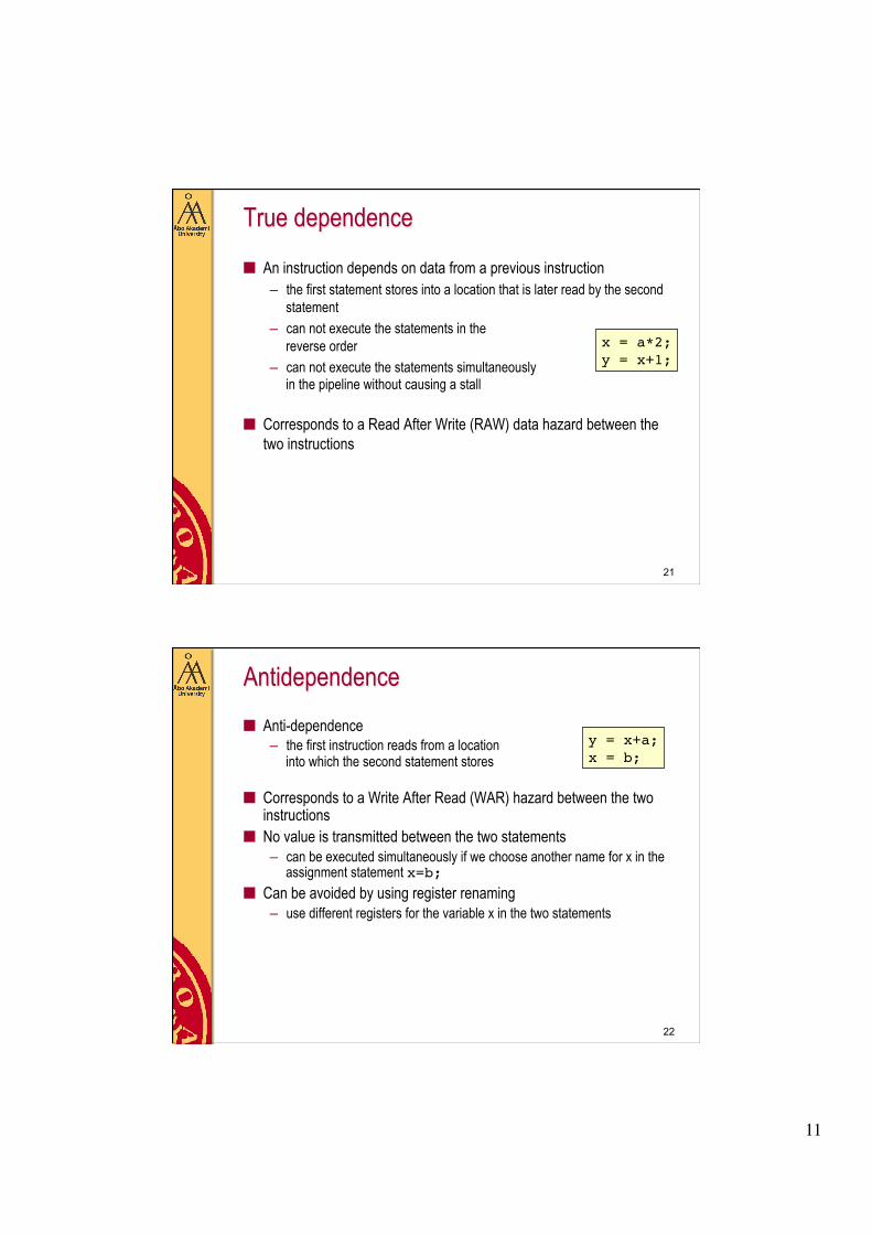
True dependence
■ An instruction depends on data from a previous instruction – the first statement stores into a location that is later read by the second
statement – can not execute the statements in the
reverse order – can not execute the statements simultaneously
in the pipeline without causing a stall
■ Corresponds to a Read After Write (RAW) data hazard between the two instructions
x = a*2;!y = x+1;!
22
Antidependence ■ Anti-dependence
– the first instruction reads from a location into which the second statement stores
■ Corresponds to a Write After Read (WAR) hazard between the two instructions
■ No value is transmitted between the two statements – can be executed simultaneously if we choose another name for x in the
assignment statement x=b; ■ Can be avoided by using register renaming
– use different registers for the variable x in the two statements
y = x+a;!x = b; !
12
23
Output dependence ■ Output dependence
– two instructions write to the same register or memory location
■ Corresponds to a Write After Write (WAW) hazard between the two instructions
■ No value is transmitted between the two statements – can be executed simultaneously if we choose another name for one of
the references to x ■ Can be avoided by using register renaming
x = x+1;! ...!x = b;!
24
Control dependence ■ Control dependence determine the order
of instructions with respect to branches (jumps) in the code – if p evaluates to TRUE, the instruction s1
is executed – if p evaluates to FALSE, the instruction s1 is not
executed, but is branched over!■ Instruction that are control dependent on a branch can not be moved
before the branch – instructions from the then-part of an if-statement can not
be executed before the branch ■ Instructions that are not control dependent on a branch can not be
moved into the then-part ■ Can avoid hazards by using branch prediction
– speculative execution
s0;!if (p)! then s1;!s2;!
13
25
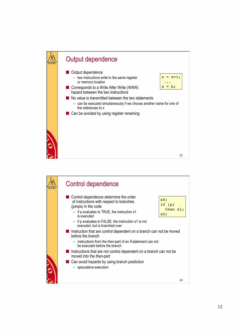
Branch prediction ■ To avoid stalling the pipeline when branch instructions are executed, branch
prediction is used – it is very important to have a good branch prediction mechanism, since branches
are very common in most programs – Example: 20% branch instructions in SPECint92 benchmark
■ Branch prediction is only needed for conditional branches, unconditional branches are always taken – subroutine calls and goto-statements are always taken – returns from subroutines need to be predicted
■ Two types of branch prediction mechanisms: – static
uses fixed rules for guessing how branches will go – dynamic
collects information about how the branches have behaved in the past, and use that to predict how the branch will go the next time
26
Mispredicted branches
■ When a misprediction occurs, the processor has executed instructions that should not be executed – it has to undo the effects of the falsely
executed instructions ■ It is not allowed to change the state of the
processor until the branch outcome is known – no writeback can be done before the outcome
of the branch is ready ■ The instructions that were executed because of a mispredicted
branch have to be undone – flush out the mispredicted instructions from the pipeline – restart the instruction fetch from the correct branch target
■ The performance penalty of a mispredicted branch is typically as many clock cycles as the length of the pipeline
if (f(x)>n)! x = 0; !else! x = 1; !. . .!
14
27
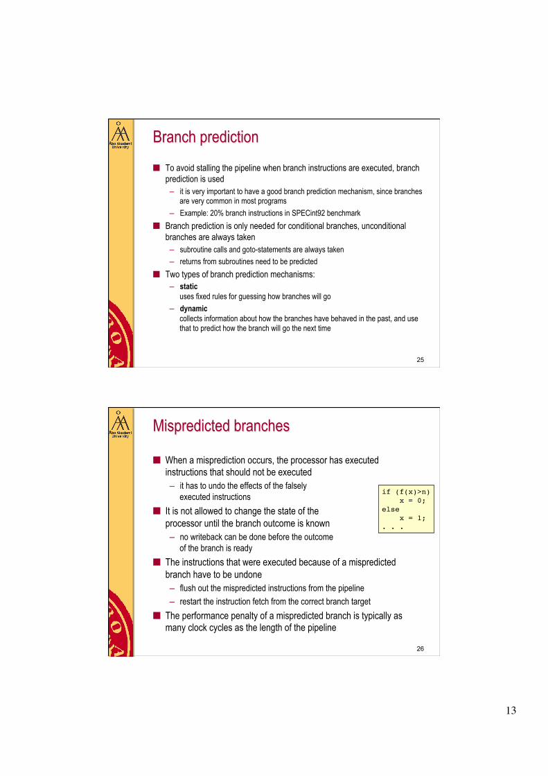
Static branch prediction
■ Fixed rules for predicting how a branch will behave – the prediction is not based on the earlier behavior of the branch – guess the outcome of the branch, and continue the execution with
the predicted instruction ■ Predict as taken / not taken
– the prediction is the same for all branches
■ Direction-based prediction – backward branches are taken – forward branches are not taken – success rate is about 65%
for (i=0; i<n; i++)!{! X[i] = 0;!)!y=1;!. . .!
28
Dynamic branch prediction
■ Static branch prediction does not consider the previous outcomes of branches – branches often show regular and repetitive patterns
■ In dynamic branch prediction the prediction is based on the outcome of previous executions of the branch – collect branch history information, on which we base the prediction
■ In practice it is not possible to store information about all branches in a program – there is no upper limit on the number of branches in a program – use a small and fast internal memory buffer to store information about
branch outcomes
15
29
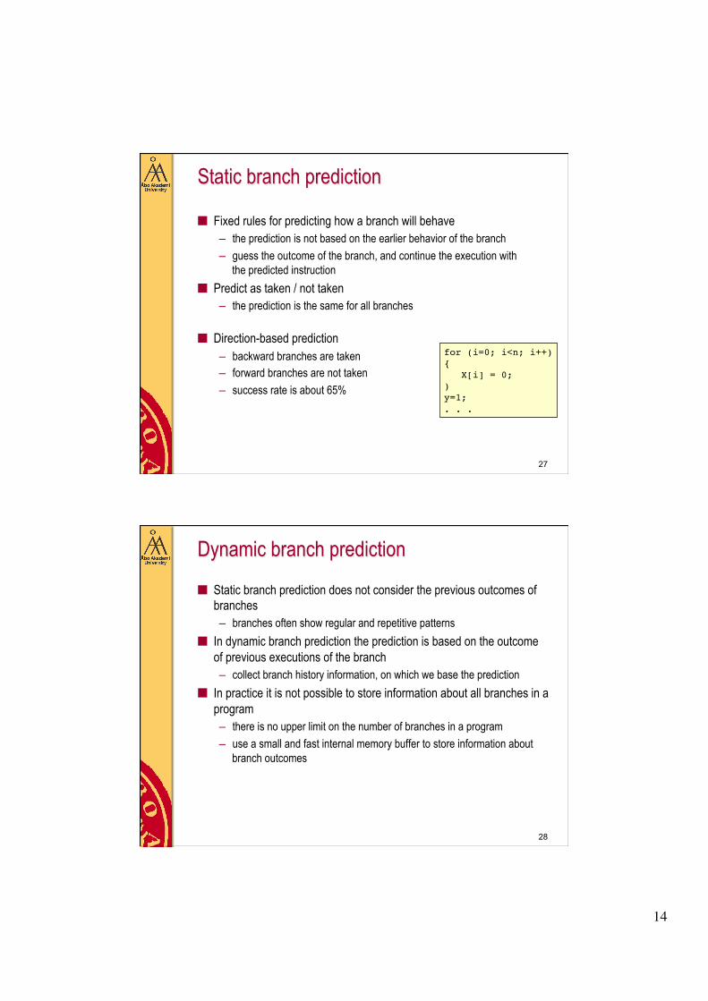
Branch history
■ Branch history information is collected in a small cache memory called the branch history table – indexed by a number of bits from the branch instruction address – contains branch history information (taken/not taken) – two branches may use the same table entry, which may lead to incorrect
predictions ■ Stores the outcome of the most recent branch executions
– need at least one bit in each table entry to store the outcome of the branch (taken / not taken)
– if no branch history exists, use static prediction ■ The branch history information is used to fetch the next instruction
from the predicted target – done in the instruction fetch/decode phase in the pipeline
30
Branch target buffer ■ The branch target buffer also stores the target address of the branch
– we can find the target address of the branch already in the instruction fetch phase
– if the branch is predicted as taken, we can immediately start fetching instructions from the branch target address
■ Implemented by associative memory
■ Only need to store information about branches that are predicted to be taken – if we find an entry in the table, it is
predicted as taken – otherwise, we predict it as not taken and continue
execution with the following instruction – used with one-bit branch history
Branch instruction address
Branch target address
Branch prediction taken / not taken
16
31
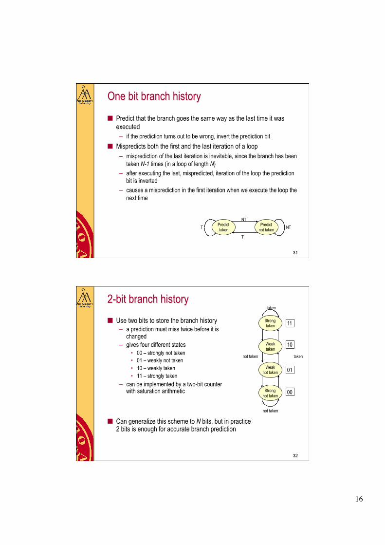
One bit branch history
■ Predict that the branch goes the same way as the last time it was executed – if the prediction turns out to be wrong, invert the prediction bit
■ Mispredicts both the first and the last iteration of a loop – misprediction of the last iteration is inevitable, since the branch has been
taken N-1 times (in a loop of length N) – after executing the last, mispredicted, iteration of the loop the prediction
bit is inverted – causes a misprediction in the first iteration when we execute the loop the
next time
Predict taken
Predict not taken
T
NT T NT
32
2-bit branch history ■ Use two bits to store the branch history
– a prediction must miss twice before it is changed
– gives four different states • 00 – strongly not taken • 01 – weakly not taken • 10 – weakly taken • 11 – strongly taken
– can be implemented by a two-bit counter with saturation arithmetic
■ Can generalize this scheme to N bits, but in practice 2 bits is enough for accurate branch prediction
Strong taken
Weak taken
Weak not taken
Strong not taken
taken not taken
00
01
10
11
taken
not taken
17
33
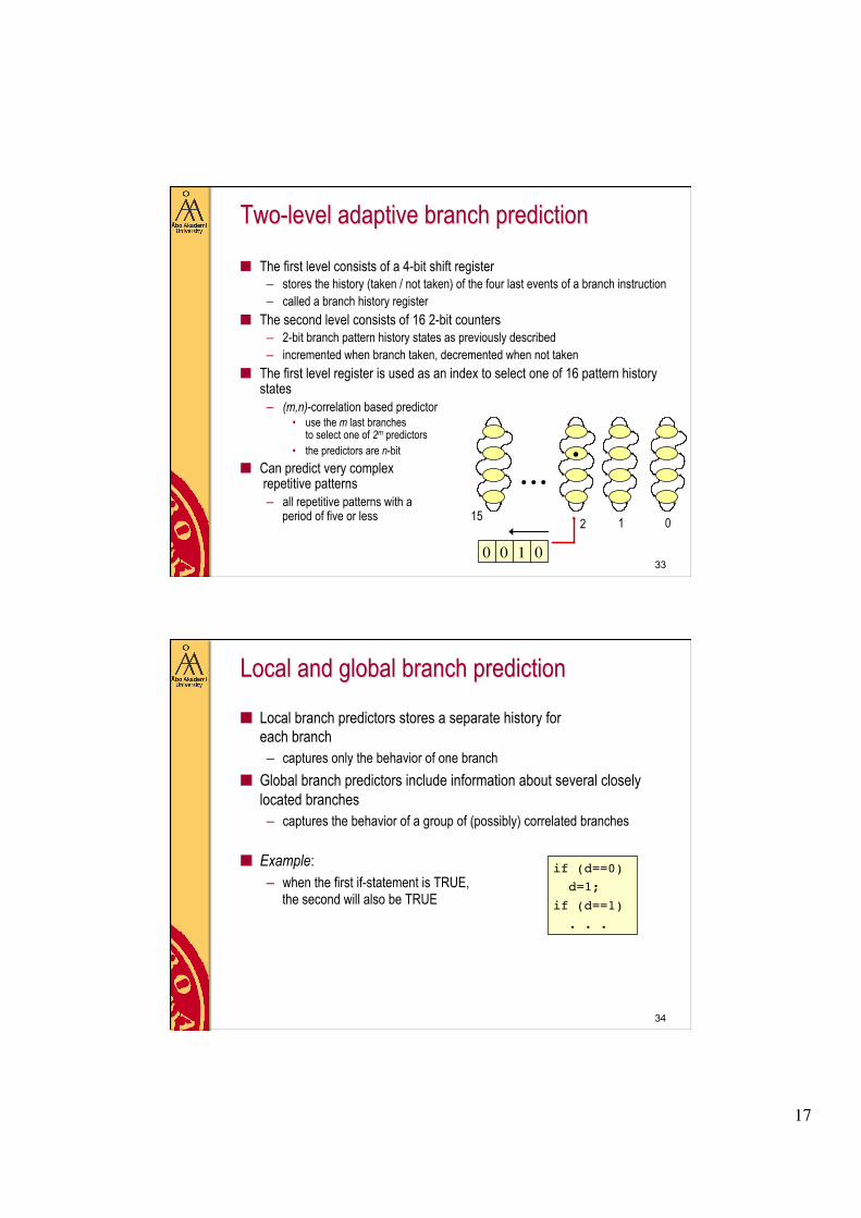
Two-level adaptive branch prediction
■ The first level consists of a 4-bit shift register – stores the history (taken / not taken) of the four last events of a branch instruction – called a branch history register
■ The second level consists of 16 2-bit counters – 2-bit branch pattern history states as previously described – incremented when branch taken, decremented when not taken
■ The first level register is used as an index to select one of 16 pattern history states – (m,n)-correlation based predictor
• use the m last branches to select one of 2m predictors
• the predictors are n-bit ■ Can predict very complex
repetitive patterns – all repetitive patterns with a
period of five or less
0 0 1 0
• ... 0 1 2 15
34
Local and global branch prediction
■ Local branch predictors stores a separate history for each branch – captures only the behavior of one branch
■ Global branch predictors include information about several closely located branches – captures the behavior of a group of (possibly) correlated branches
■ Example:
– when the first if-statement is TRUE, the second will also be TRUE
if (d==0) ! d=1;!if (d==1)! . . .!
18
35
Tournament branch predictor
■ Multilevel branch predictor, which uses more than one branch prediction method – chooses the method that previously has given the best result for each
branch – stores for each branch a selector to one of the methods, for instance
using a 1-bit saturating counter ■ Combines both local and global predictors, and uses the method that is
best for each branch ■ Requires more resources than simpler branch prediction methods
– more internal tables to maintain – more complex decision mechanism
36
Predicting call/returns
■ Procedure calls are unconditional branches – always taken – procedure returns need to be predicted
■ Procedure calls and returns are paired – one return for each procedure call – can have nested procedure calls
■ Use a return address stack (RAS) as a branch target buffer to predict the return address – push the return address when the call instruction is executed – pop it when the return instruction is executed
■ Using advanced adaptive branch prediction mechanisms of this kind, it
is possible to achieve up to 95% accuracy – performance depends strongly on the code
19
37
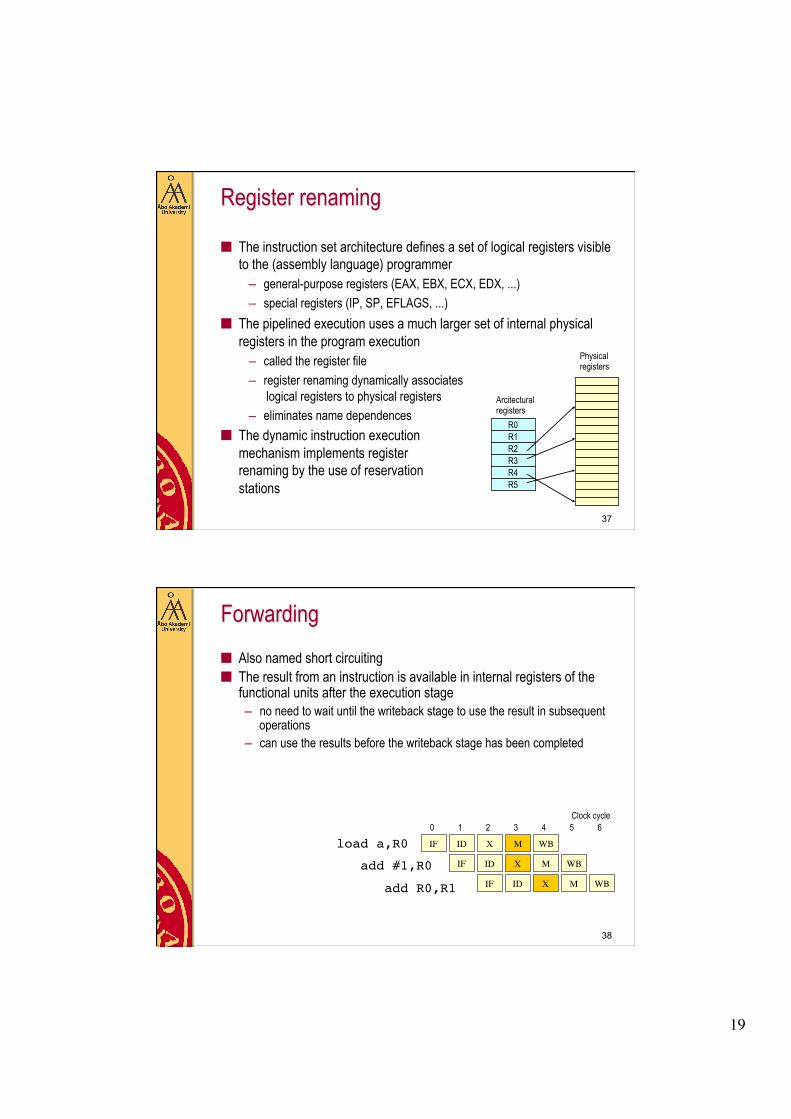
Register renaming
■ The instruction set architecture defines a set of logical registers visible to the (assembly language) programmer
– general-purpose registers (EAX, EBX, ECX, EDX, ...) – special registers (IP, SP, EFLAGS, ...)
■ The pipelined execution uses a much larger set of internal physical registers in the program execution
– called the register file – register renaming dynamically associates
logical registers to physical registers – eliminates name dependences
■ The dynamic instruction execution mechanism implements register renaming by the use of reservation stations
R0 R1 R2 R3 R4 R5
Arcitectural registers
Physical registers
38
Forwarding ■ Also named short circuiting ■ The result from an instruction is available in internal registers of the
functional units after the execution stage – no need to wait until the writeback stage to use the result in subsequent
operations – can use the results before the writeback stage has been completed
IF ID M WB X
IF ID M WB X
X IF ID M WB
Clock cycle 0 1 2 3 4 5 6
load a,R0!
add #1,R0!
add R0,R1!
20
39
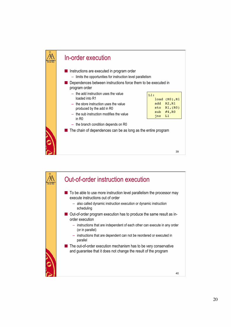
In-order execution
■ Instructions are executed in program order – limits the opportunities for instruction level parallelism
■ Dependences between instructions force them to be executed in program order – the add instruction uses the value
loaded into R1 – the store instruction uses the value
produced by the add in R0 – the sub instruction modifies the value
in R0 – the branch condition depends on R0
■ The chain of dependences can be as long as the entire program
L1:! load (R0),R1! add R2,R1! sto R1,(R0)! sub #4,R0! jnz L1!
40
Out-of-order instruction execution
■ To be able to use more instruction level parallelism the processor may execute instructions out of order
– also called dynamic instruction execution or dynamic instruction scheduling
■ Out-of-order program execution has to produce the same result as in-order execution
– instructions that are independent of each other can execute in any order (or in parallel)
– instructions that are dependent can not be reordered or executed in parallel
■ The out-of-order execution mechanism has to be very conservative and guarantee that it does not change the result of the program
21
41
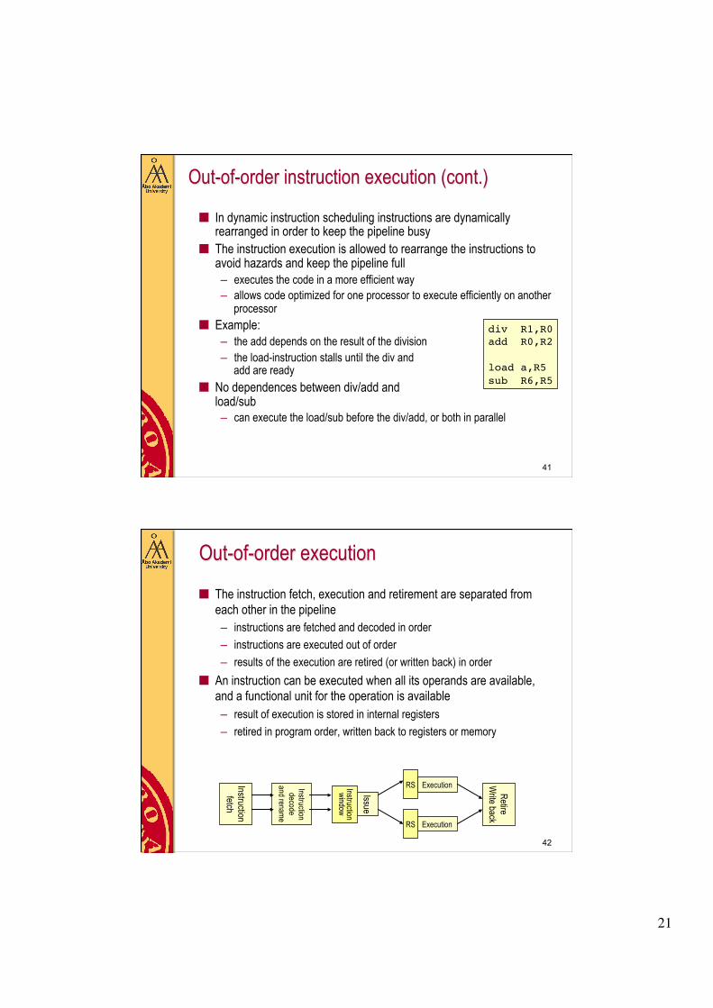
Out-of-order instruction execution (cont.)
■ In dynamic instruction scheduling instructions are dynamically rearranged in order to keep the pipeline busy
■ The instruction execution is allowed to rearrange the instructions to avoid hazards and keep the pipeline full – executes the code in a more efficient way – allows code optimized for one processor to execute efficiently on another
processor ■ Example:
– the add depends on the result of the division – the load-instruction stalls until the div and
add are ready ■ No dependences between div/add and
load/sub – can execute the load/sub before the div/add, or both in parallel
div R1,R0!add R0,R2!!load a,R5!sub R6,R5!
42
Out-of-order execution
■ The instruction fetch, execution and retirement are separated from each other in the pipeline – instructions are fetched and decoded in order – instructions are executed out of order – results of the execution are retired (or written back) in order
■ An instruction can be executed when all its operands are available, and a functional unit for the operation is available – result of execution is stored in internal registers – retired in program order, written back to registers or memory
Instruction fetch
Instruction decode
and rename
Issue
Instruction window
Retire W
rite back
Execution RS
RS Execution
22
43
Tomasulo’s algorithm ■ Method for dynamic instruction scheduling
– implements out-of-order instruction execution – R.M. Tomasulo, An Efficient Algorithm for Exploiting Multiple Arithmetic Units,
IBM J. of Res.&Dev. 11:1 (Jan 1967) – developed for IBM 360/91
■ Similar out-of-order execution mechanisms are used in most current processors
■ Avoids pipeline stalls due to dependences – instructions whose operands are available can execute out of order
■ Combines – register renaming – out-of-order instruction execution – data forwarding (short circuiting)
44
Reservation stations
■ Buffers for operands of instructions that are waiting to be issued – fetches and stores operands as soon as they are available – replaces the registers in the instruction execution – implements register
renaming – operands are identified by a unique tag – if an operand has not yet been computed, the reservation station
designates which other reservation station will produce the operand ■ Eliminates the need to fetch/write operands from/to registers
– don’t have to write results back to registers which will be immediately read by another instruction
– implements register renaming – performs the same function as forwarding (short-circuiting)
■ There are more reservation stations than registers
23
45
Reservation stations (cont.) ■ Reservation stations, functional units and
load/store buffers are connected by a Common Data Bus (CDB) – memory access (load/store) are treated
as functional units ■ When the operands of an instruction are
available, the instruction can be sent to a functional unit for execution
■ Results of execution are broadcasted on the CDB ■ Reservation stations listen to the CDB for operand values
– if a matching tag is seen on the bus, the RS copies the value into its operand field
– all reservation stations waiting for the value are updated at the same time ■ Implemented by associative memory
– can immediately identify a tag value on the CDB that it is waiting for
Reservation stations
Common Data Bus
Functional unit
46
Organization of Tomasulo’s algorithm
Load buffer
From memory
Store buffer
To memory
Reservation stations
Adder Multiplier
Common Data Bus
Registers
Instructions
Instruction fetch
Reorder buffer
24
47
Data structures in Tomasulos algorithm
■ Have to store data describing the state of instructions in reservation stations, registers and load/store buffers
■ Tags identify entries in reservation stations – used as names for an extended set of registers – points to the reservation station that holds or that will produce a result
needed as an operand in an instruction – also used to order the executed instructions in program order when they are
retired ■ Issued instructions refer to the operands by tag values
– not by the register names ■ Registers need one additional field
– the tag of the reservation station that will produce the result to be stored in this register
– if zero, no currently active instruction is computing a result destined for this register
48
Stages in Tomasulo’s algorithm ■ Issue
– get the next instruction from the instruction queue – get a free reservation station and assign the instruction and its operands
to it, if they are available in registers – if the operands are not available in registers, assign as operands the
reservation stations that will produce them – if there is no free reservation station, there is a structural hazard and the
instruction must stall until one becomes available ■ Execution
– if the operands are not ready, monitor the CDB and wait for the operands to be computed
– when the operands are ready, place them into the corresponding reservation stations
– dispatch the instruction to the functional unit for execution
25
49
Stages in Tomasulo’s algorithm ■ Write result
– after an instruction is executed, broadcast the result on the CDB – all reservation stations that are waiting for this as an operand will
receive it – mark the reservation station as free
■ Instruction retirement is done in program order
– has to produce exactly the same result as in in-order execution
■ Loads and stores may require additional steps, as they also have to compute the effective address
50
64-bit architectures
■ Today, most server, desktop and even portable computers are equipped with a 64-bit processor – can run both in 32- and 64-bit mode
■ Intel 64 and AMD64 are 64-bit Instruction Set Architectures – compatible with each other, some minor differences – collectively referred to as x86-64 ISA – backwards compatible with the 32-bit ISA IA-32
■ Other 64-bit architectures – Intel IA-64, Alpha, Sun SPARC64, IBM Power, HP PA-RISC, MIPS
■ Most modern operating systems run in 64-bit mode ■ Most compilers can generate 64-bit code
26
51
Advantages of 64-bit architectures ■ Long integers are 64 bits
– can represent integer values from -263 to +263-1 – dynamic range is about 1.8 * 1019
■ Pointers are 64 bits – can theoretically address 16 Exabyte of main memory
(that is about 18.4 * 1018 bytes) – current 64-bit systems use 48 address bits – can support 256 TB of
memory ■ Floating-point values are represented the same way both in 32- and
64-bit architectures – defined by the IEEE 754 standard – float: 32 bits, double: 64 bits, long double: 80 bits
■ All other numerical values are stored in the same way in 32- and 64-bit architectures
52
64-bit extended register sets
■ In the x86-64 architecture the number of general-purpose registers is extended from 8 to 16 – also extended in length from 32 to 64 bits – similarly, the number of XMM registers are extended
from 8 to 16 ■ 64-bit architectures have more registers
– much more of the program state can be kept is fast registers – less need to access local variables on the stack – more procedure arguments (up to 6) can be passed in registers
■ More efficient procedure call mechanism – less register pressure – compilers can generate more compact code
27
53
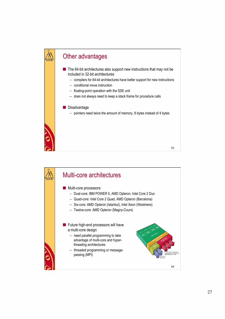
Other advantages
■ The 64-bit architectures also support new instructions that may not be included in 32-bit architectures – compilers for 64-bit architectures have better support for new instructions – conditional move instruction – floating-point operation with the SSE unit – does not always need to keep a stack frame for procedure calls
■ Disadvantage – pointers need twice the amount of memory, 8 bytes instead of 4 bytes
54
Multi-core architectures
■ Multi-core processors – Dual-core: IBM POWER 5, AMD Opteron, Intel Core 2 Duo – Quad-core: Intel Core 2 Quad, AMD Opteron (Barcelona) – Six-core: AMD Opteron (Istanbul), Intel Xeon (Westmere) – Twelve-core: AMD Opteron (Magny-Cours)
■ Future high-end processors will have a multi-core design – need parallel programming to take
advantage of multi-core and hyper- threading architectures
– threaded programming or message- passing (MPI)
28
55
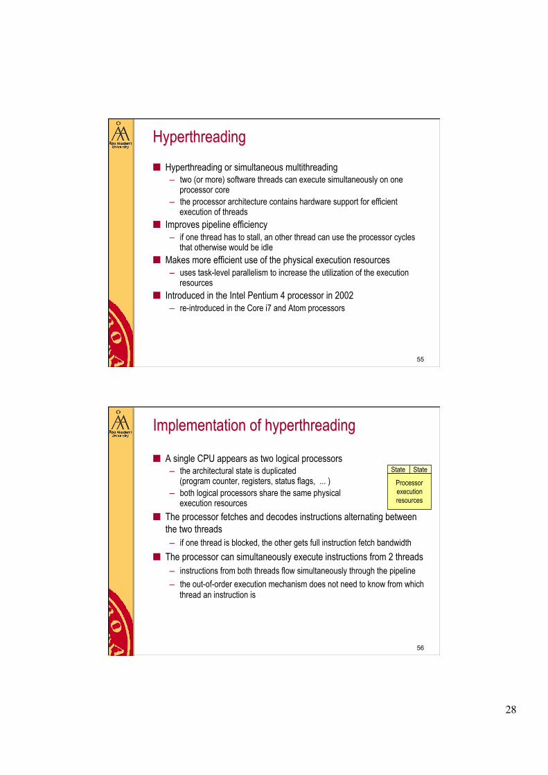
Hyperthreading ■ Hyperthreading or simultaneous multithreading
– two (or more) software threads can execute simultaneously on one processor core
– the processor architecture contains hardware support for efficient execution of threads
■ Improves pipeline efficiency – if one thread has to stall, an other thread can use the processor cycles
that otherwise would be idle ■ Makes more efficient use of the physical execution resources
– uses task-level parallelism to increase the utilization of the execution resources
■ Introduced in the Intel Pentium 4 processor in 2002 – re-introduced in the Core i7 and Atom processors
56
Implementation of hyperthreading
■ A single CPU appears as two logical processors – the architectural state is duplicated
(program counter, registers, status flags, ... ) – both logical processors share the same physical
execution resources ■ The processor fetches and decodes instructions alternating between
the two threads – if one thread is blocked, the other gets full instruction fetch bandwidth
■ The processor can simultaneously execute instructions from 2 threads – instructions from both threads flow simultaneously through the pipeline – the out-of-order execution mechanism does not need to know from which
thread an instruction is
Processor execution resources
State State
29
57
Processor architectures for embedded systems ■ Processors for embedded systems are intended to be used in
consumer products, wireless and networking devices, handheld and mobile devices, automotive industry, etc.
■ Puts very special requirements on the processor architecture – broad range of performance requirements
• from very small 8- or 16-bit processors to 32- or 64-bit processors with advanced signal processing capabilities
• must be available in a large number of different configurations – low power consumption and heat dissipation – low cost, high flexibility – available also as a processor core which can be integrated with other
hardware on the same chip – small physical footprint (nr. of transistors)
58
Embedded systems processors
■ Example of an ISA for embedded processors: ARMv6 – backwards compatible with previous generations of ARM processors
■ Characteristics of the microarchitecture – short pipeline – low clock frequency – scalar processor design
• issues one instruction in each clock cycle, in-order execution • a few separate functional units (e.g. ALU, Multiply/Add and Load/Store)
– simple branch prediction mechanism (static and dynamic) – small cache size
• can choose between a number of alternative cache sizes – SIMD instructions for media processing
30
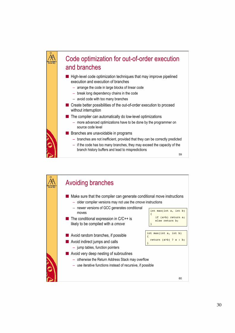
Code optimization for out-of-order execution and branches ■ High-level code optimization techniques that may improve pipelined
execution and execution of branches – arrange the code in large blocks of linear code – break long dependency chains in the code – avoid code with too many branches
■ Create better possibilities of the out-of-order execution to proceed without interruption
■ The compiler can automatically do low-level optimizations – more advanced optimizations have to be done by the programmer on
source code level ■ Branches are unavoidable in programs
– branches are not inefficient, provided that they can be correctly predicted – if the code has too many branches, they may exceed the capacity of the
branch history buffers and lead to mispredictions 59
Avoiding branches
■ Make sure that the compiler can generate conditional move instructions – older compiler versions may not use the cmove instructions – newer versions of GCC generates conditional
moves ■ The conditional expression in C/C++ is
likely to be compiled with a cmove
■ Avoid random branches, if possible ■ Avoid indirect jumps and calls
– jump tables, function pointers ■ Avoid very deep nesting of subroutines
– otherwise the Return Address Stack may overflow – use iterative functions instead of recursive, if possible
60
int max(int a, int b)!{! return (a>b) ? a : b;!} !
int max(int a, int b)!{! if (a>b) return a;! else return b;!} !
31
Branch density
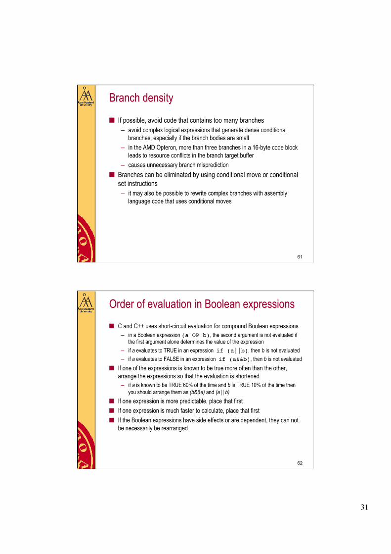
■ If possible, avoid code that contains too many branches – avoid complex logical expressions that generate dense conditional
branches, especially if the branch bodies are small – in the AMD Opteron, more than three branches in a 16-byte code block
leads to resource conflicts in the branch target buffer – causes unnecessary branch misprediction
■ Branches can be eliminated by using conditional move or conditional set instructions – it may also be possible to rewrite complex branches with assembly
language code that uses conditional moves
61
Order of evaluation in Boolean expressions ■ C and C++ uses short-circuit evaluation for compound Boolean expressions
– in a Boolean expression (a OP b), the second argument is not evaluated if the first argument alone determines the value of the expression
– if a evaluates to TRUE in an expression if (a||b), then b is not evaluated – if a evaluates to FALSE in an expression if (a&&b), then b is not evaluated
■ If one of the expressions is known to be true more often than the other, arrange the expressions so that the evaluation is shortened – if a is known to be TRUE 60% of the time and b is TRUE 10% of the time then
you should arrange them as (b&&a) and (a || b) ■ If one expression is more predictable, place that first ■ If one expression is much faster to calculate, place that first ■ If the Boolean expressions have side effects or are dependent, they can not
be necessarily be rearranged
62
32
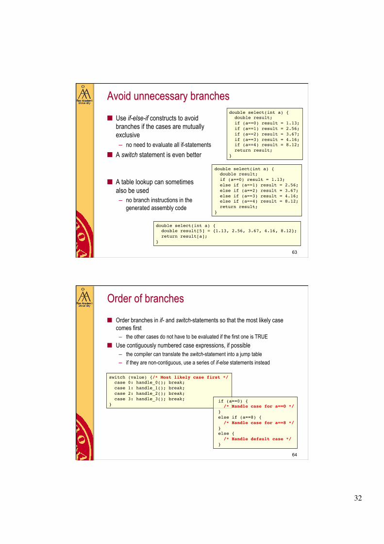
Avoid unnecessary branches
■ Use if-else-if constructs to avoid branches if the cases are mutually exclusive – no need to evaluate all if-statements
■ A switch statement is even better
■ A table lookup can sometimes also be used – no branch instructions in the
generated assembly code
63
double select(int a) {! double result;! if (a==0) result = 1.13; ! if (a==1) result = 2.56;! if (a==2) result = 3.67;! if (a==3) result = 4.16;! if (a==4) result = 8.12;! return result;!}!
double select(int a) {! double result;! if (a==0) result = 1.13;! else if (a==1) result = 2.56;! else if (a==2) result = 3.67;! else if (a==3) result = 4.16;! else if (a==4) result = 8.12;! return result;!}!
double select(int a) {! double result[5] = {1.13, 2.56, 3.67, 4.16, 8.12};! return result[a];!}!
Order of branches ■ Order branches in if- and switch-statements so that the most likely case
comes first – the other cases do not have to be evaluated if the first one is TRUE
■ Use contiguously numbered case expressions, if possible – the compiler can translate the switch-statement into a jump table – if they are non-contiguous, use a series of if-else statements instead
64
switch (value) {/* Most likely case first */! case 0: handle_0(); break; ! case 1: handle_1(); break;! case 2: handle_2(); break;! case 3: handle_3(); break;!}!
if (a==0) {! /* Handle case for a==0 */! }! else if (a==8) {! /* Handle case for a==8 */! }! else {! /* Handle default case */! }!
33
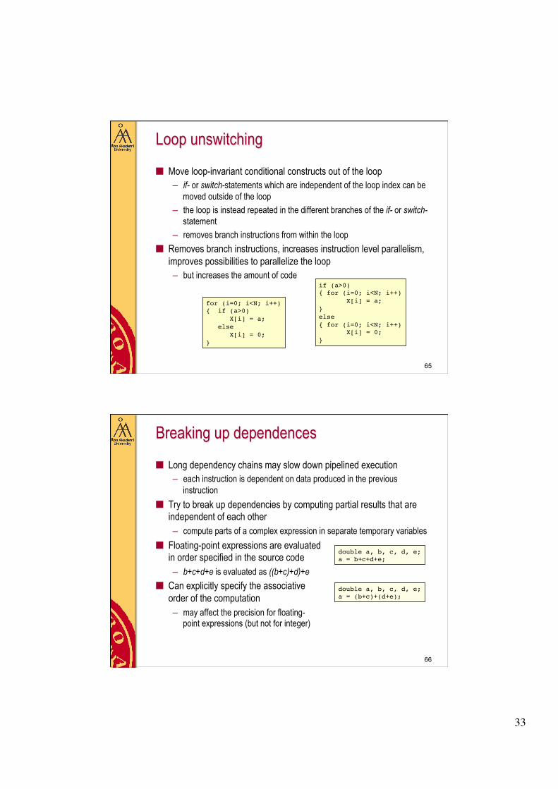
Loop unswitching
■ Move loop-invariant conditional constructs out of the loop – if- or switch-statements which are independent of the loop index can be
moved outside of the loop – the loop is instead repeated in the different branches of the if- or switch-
statement – removes branch instructions from within the loop
■ Removes branch instructions, increases instruction level parallelism, improves possibilities to parallelize the loop – but increases the amount of code
65
for (i=0; i<N; i++)!{ if (a>0)! X[i] = a;! else! X[i] = 0;!}!
if (a>0)!{ for (i=0; i<N; i++)! X[i] = a;!}!else!{ for (i=0; i<N; i++)! X[i] = 0;!}!
Breaking up dependences
■ Long dependency chains may slow down pipelined execution – each instruction is dependent on data produced in the previous
instruction ■ Try to break up dependencies by computing partial results that are
independent of each other – compute parts of a complex expression in separate temporary variables
■ Floating-point expressions are evaluated in order specified in the source code – b+c+d+e is evaluated as ((b+c)+d)+e
■ Can explicitly specify the associative order of the computation – may affect the precision for floating-
point expressions (but not for integer)
66
double a, b, c, d, e; !a = b+c+d+e;!
double a, b, c, d, e; !a = (b+c)+(d+e);!
34
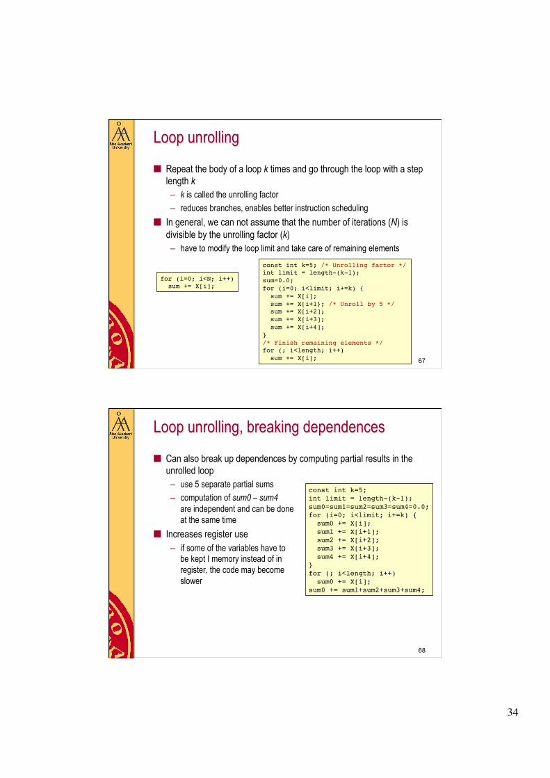
Loop unrolling
■ Repeat the body of a loop k times and go through the loop with a step length k – k is called the unrolling factor – reduces branches, enables better instruction scheduling
■ In general, we can not assume that the number of iterations (N) is divisible by the unrolling factor (k) – have to modify the loop limit and take care of remaining elements
67
for (i=0; i<N; i++)! sum += X[i];!
const int k=5; /* Unrolling factor */!int limit = length-(k-1);!sum=0.0;!for (i=0; i<limit; i+=k) {! sum += X[i];! sum += X[i+1}; /* Unroll by 5 */! sum += X[i+2];! sum += X[i+3];! sum += X[i+4];!}!/* Finish remaining elements */!for (; i<length; i++)! sum += X[i];!
Loop unrolling, breaking dependences
■ Can also break up dependences by computing partial results in the unrolled loop – use 5 separate partial sums – computation of sum0 – sum4
are independent and can be done at the same time
■ Increases register use – if some of the variables have to
be kept I memory instead of in register, the code may become slower
68
const int k=5; !int limit = length-(k-1);!sum0=sum1=sum2=sum3=sum4=0.0;!for (i=0; i<limit; i+=k) {! sum0 += X[i];! sum1 += X[i+1];! sum2 += X[i+2];! sum3 += X[i+3];! sum4 += X[i+4];!}!for (; i<length; i++)! sum0 += X[i];!sum0 += sum1+sum2+sum3+sum4;!
35
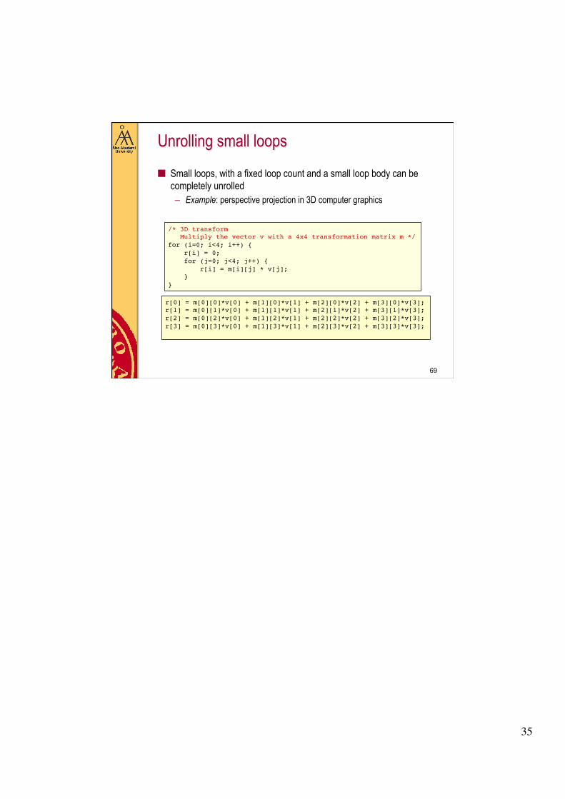
Unrolling small loops
■ Small loops, with a fixed loop count and a small loop body can be completely unrolled – Example: perspective projection in 3D computer graphics
69
/* 3D transform! Multiply the vector v with a 4x4 transformation matrix m */ !for (i=0; i<4; i++) {! r[i] = 0;! for (j=0; j<4; j++) {! r[i] = m[i][j] * v[j];! }!}!
r[0] = m[0][0]*v[0] + m[1][0]*v[1] + m[2][0]*v[2] + m[3][0]*v[3];!r[1] = m[0][1]*v[0] + m[1][1]*v[1] + m[2][1]*v[2] + m[3][1]*v[3];!r[2] = m[0][2]*v[0] + m[1][2]*v[1] + m[2][2]*v[2] + m[3][2]*v[3];!r[3] = m[0][3]*v[0] + m[1][3]*v[1] + m[2][3]*v[2] + m[3][3]*v[3];!!