Microsoft Excel 2010 - Dashboard

Microsoft

Excel 2010

Fundamentals

Evaluation Copy

Written By:

Jeff Hutchinson [email protected] http://www.excel-networks.com

Page ii Excel 2010-Fundamentals Rev: 1.0 Date: 7/24/2011

Introduction

Course Description

This introductory class will cover 4 major topics. They will explain how to use features in

Excel such as navigation, formulas, formatting and printing. In order to navigate Excel, you

can use the mouse to select information, and the keyboard to move and manipulate data as

well as adjust ranges to move and copy large groups of data. Creating formulas is a primary

aspect of using Excel and you will learn how to create, calculate, and check formula results.

In order to make the document look professional, you will need to format numbers, text,

borders, and cells. In order to produce a final output, you will need to setup the headers,

footers, page layout, and print a selected area.

Prerequisite

It is helpful to have a working knowledge of computers, but it is not required to take this class.

Course Outline Day 1 - Navigation

Chapter 1 - Exploring Excel Chapter 2 – Navigation Techniques Chapter 3 – Excel Worksheets Chapter 4 – Selection And Entering Text Chapter 5 – Fill Handle

Day 2 - Formulas and Functions

Chapter 6 - Creating Simple Formulas Chapter 7 - Copying And Moving Data Day 3 - Formatting

Chapter 8 - Formatting Numbers Chapter 9 - Formatting Text Chapter 10 - Formatting Cells Chapter 11 - Working With Columns And Rows Chapter 12 - Printing A Spreadsheet

Optional

Appendix A - Creating Charts Appendix B – Keyboard Shortcuts Appendix C – End Of Class Project

Learning Process

All modules in this course will follow these basic steps for learning:

Theoretical discussion of the topic.

Example of a topic in a presentation.

Step-by-step completion of the topic as a class.

Practice to review skills located at the end of the chapter.

Homework is recommended to better understand the concepts.

Page iv Excel 2010-Fundamentals Rev: 1.0 Date: 7/24/2011

Highlights in Document

Commands, keyboard combinations and specific menu choices are highlighted in bold.

These are the most important text statements in the Step-By-Step and Practice Exercises.

For example, the word “Insert” bolded text (Example: Insert ribbon tab) is the most

important statement in the text string and “Shift F1” is a keyboard command that is

highlighted for emphasis.

About the Author

Jeff Hutchinson is a computer instructor teaching a variety of classes around the country.

He has a BS degree from BYU in Computer Aided Engineering and has worked in the

Information Technology field supporting and maintaining computers for many years. He

also owned a computer training and consulting firm in San Francisco, California. After

selling his business in 2001, he continued to work as an independent computer instructor

in California and Utah. Jeff Hutchinson lives in Utah and provides training for the Utah

Valley University Community Education system, offering valuable computer skills for

the general knowledge of students, career development, and career advancement.

Understanding the technology and the needs of the students has been the basis for

developing this material. Jeff Hutchinson can be contacted at

[email protected] or (801) 376-6687.

Released Version

This documentation is based on Microsoft Excel 2010. The latest revision of this

Introductory book is Excel 2010-Fundamentals Rev: 1.0 Date: 7/24/2011

Copyright

This material is the sole property of Jeff Hutchinson through his company Excel

Networks. Any copying, duplication or reproduction of this document must be approved

by Jeff Hutchinson in writing. However, students can use the material in and out of class

for personal development and learning.

mailto:[email protected]

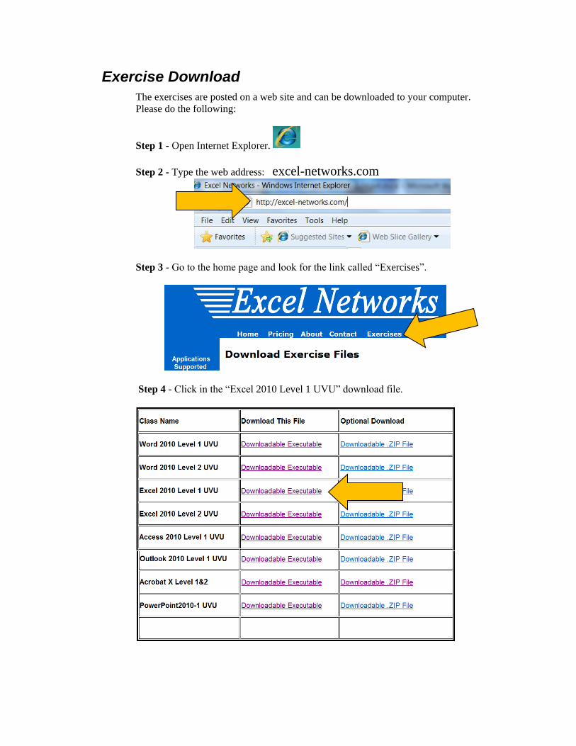
Exercise Download

The exercises are posted on a web site and can be downloaded to your computer.

Please do the following:

Step 1 - Open Internet Explorer.

Step 2 - Type the web address: excel-networks.com

Step 3 - Go to the home page and look for the link called “Exercises”.

Step 4 - Click in the “Excel 2010 Level 1 UVU” download file.

Page vi Excel 2010-Fundamentals Rev: 1.0 Date: 7/24/2011

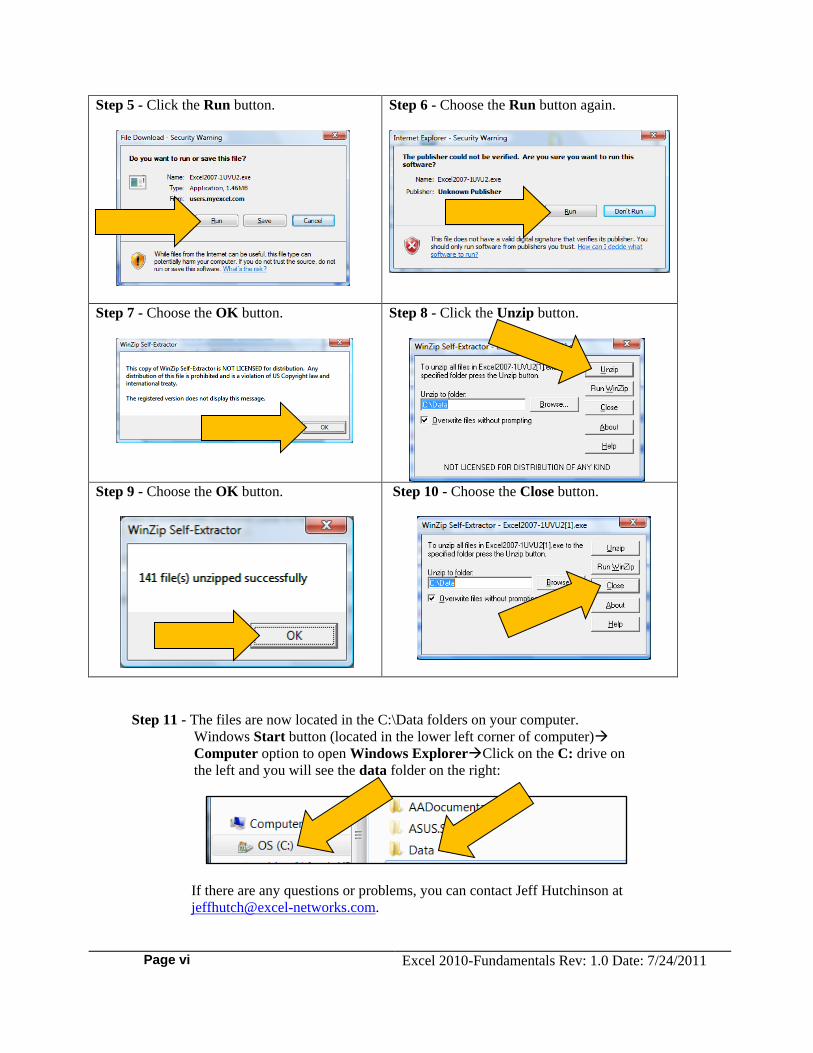
Step 5 - Click the Run button.

Step 6 - Choose the Run button again.

Step 7 - Choose the OK button.

Step 8 - Click the Unzip button.

Step 9 - Choose the OK button.

Step 10 - Choose the Close button.

Step 11 - The files are now located in the C:\Data folders on your computer.

Windows Start button (located in the lower left corner of computer)

Computer option to open Windows ExplorerClick on the C: drive on

the left and you will see the data folder on the right:

If there are any questions or problems, you can contact Jeff Hutchinson at

[email protected].

mailto:[email protected]

Table of Contents Excel 2010 - Fundamentals

INTRODUCTION ...................................................................................................... I Course Description ................................................................................................. iii Prerequisite ............................................................................................................. iii Course Outline ........................................................................................................ iii Learning Process .................................................................................................... iii Highlights in Document ......................................................................................... iv About the Author .................................................................................................... iv Released Version .................................................................................................... iv Copyright ................................................................................................................ iv Exercise Download ................................................................................................... v

CHAPTER 1 - EXPLORING EXCEL ...................................................................... 1 1.1 Opening a Workbook ......................................................................................... 1 1.2 Saving, Closing, Opening and Creating a Workbook......................................... 1 1.3 Using a Template ................................................................................................ 2 1.4 The Ribbon ......................................................................................................... 3 1.5 Contextual Ribbon Tabs ..................................................................................... 5 1.6 Galleries .............................................................................................................. 6 1.7 Dialog Box Launcher ......................................................................................... 6 1.8 Quick Access Toolbar ........................................................................................ 7 1.9 Hiding the Ribbon .............................................................................................. 8 1.10 Minimize/Maximize Buttons ............................................................................ 8 1.11 Formula Bar ...................................................................................................... 9 1.12 File Ribbon Tab ................................................................................................ 9 1.13 Pinning Files ................................................................................................... 10 1.14 Application Options ........................................................................................ 11 1.15 Using the Mini Toolbar .................................................................................. 13 1.16 Status Bar ....................................................................................................... 14 Practice1 Exercise - Exploring Excel ..................................................................... 15

CHAPTER 2 – NAVIGATION TECHNIQUES .................................................... 17 2.1 Keyboard Commands ....................................................................................... 17 2.2 Using KeyTips .................................................................................................. 17 2.3 Using the Mouse on the Scroll Bar ................................................................... 18 2.4 Scroll Bar Shortcut Menu ................................................................................. 19 2.5 Mouse Drag ...................................................................................................... 20 2.6 Zoom Slider and View ribbon tab .................................................................... 20 Practice1 Exercise - Exploring Excel ..................................................................... 21

CHAPTER 3 – EXCEL WORKSHEETS ERROR! BOOKMARK NOT DEFINED. 3.1 Navigating Between Worksheets...................... Error! Bookmark not defined. 3.2 Selecting and Moving Worksheets ................... Error! Bookmark not defined. 3.3 Renaming Worksheets ...................................... Error! Bookmark not defined. 3.4 Worksheet Options ........................................... Error! Bookmark not defined. 3.5 Selecting Multiple Worksheets ......................... Error! Bookmark not defined. Practice1 Exercise – Working with Worksheets .... Error! Bookmark not defined. Practice2 Exercise - Worksheet Tabs ..................... Error! Bookmark not defined.

CHAPTER 4 – SELECTION AND ENTERING TEXTERROR! BOOKMARK NOT

DEFINED. 4.1 Entering Text .................................................... Error! Bookmark not defined.

Page viii Excel 2010-Fundamentals Rev: 1.0 Date: 7/24/2011

4.2 Entering Numbers into Cells ............................ Error! Bookmark not defined. 4.3 Using Data Entry Shortcuts .............................. Error! Bookmark not defined. 4.4 Selecting Ranges with the Mouse ..................... Error! Bookmark not defined. 4.5 Selecting Ranges with the Keyboard ................ Error! Bookmark not defined. 4.6 Selecting Non-adjacent Ranges ........................ Error! Bookmark not defined. 4.7 Entering Values into a Range ........................... Error! Bookmark not defined. Practice1 Exercise - Using Basic Workbook Skills Error! Bookmark not defined.

CHAPTER 5 – FILL HANDLE ............... ERROR! BOOKMARK NOT DEFINED. 5.1 Using the Auto Fill Feature .............................. Error! Bookmark not defined. 5.2 Using the Fill Handle Options .......................... Error! Bookmark not defined. 5.3 Using the Auto Fill Patterns ............................. Error! Bookmark not defined. Practice1 Exercise - Working with Ranges ............ Error! Bookmark not defined.

CHAPTER 6 - CREATING SIMPLE FORMULASERROR! BOOKMARK NOT DEFINED. 6.1 Using Formulas ................................................ Error! Bookmark not defined. 6.2 Entering Formulas by Typing ........................... Error! Bookmark not defined. 6.3 Entering Formulas by using the Mouse ............ Error! Bookmark not defined. 6.4 Manually Typed Functions ............................... Error! Bookmark not defined. 6.5 Using the AutoSum Button............................... Error! Bookmark not defined. 6.6 Using the AutoSum list .................................... Error! Bookmark not defined. 6.7 Using Formula AutoComplete .......................... Error! Bookmark not defined. 6.8 Inserting Functions in Formulas ....................... Error! Bookmark not defined. 6.9 Editing Functions .............................................. Error! Bookmark not defined. 6.10 Using the AutoCalculate Feature .................... Error! Bookmark not defined. 6.11 Using Range Borders to Modify Formulas ..... Error! Bookmark not defined. 6.12 Autocorrect Feature ........................................ Error! Bookmark not defined. Practice1 Exercise - Practice Using Previous ExerciseError! Bookmark not defined. Practice2 Exercise - Creating Simple Formulas .... Error! Bookmark not defined. Practice3 Exercise - Creating Simple Formulas ..... Error! Bookmark not defined. Practice4 Exercise - Creating Simple Formulas ..... Error! Bookmark not defined. Practice5 Exercise - Creating Simple Formulas ..... Error! Bookmark not defined.

CHAPTER 7 - COPYING AND MOVING DATAERROR! BOOKMARK NOT DEFINED. 7.1 Copying/Cutting and Pasting Data ................... Error! Bookmark not defined. 7.2 Copying and Pasting Formulas ......................... Error! Bookmark not defined. 7.3 Creating an Absolute Reference ....................... Error! Bookmark not defined. 7.4 Using Drag-and-Drop Editing .......................... Error! Bookmark not defined. 7.5 Using Undo and Redo ...................................... Error! Bookmark not defined. Practice1 Exercise – Keyboard Copy and Paste ..... Error! Bookmark not defined. Practice2 Exercise - Copying and Moving Data..... Error! Bookmark not defined.

CHAPTER 8 - FORMATTING NUMBERSERROR! BOOKMARK NOT DEFINED. 8.1 Accounting and Currency Number Style .......... Error! Bookmark not defined. 8.2 Using the Percent Style .................................... Error! Bookmark not defined. 8.3 Using the Comma Style .................................... Error! Bookmark not defined. 8.4 Changing Decimal Places ................................. Error! Bookmark not defined. Practice1 Exercise - Formatting Numbers .............. Error! Bookmark not defined.

CHAPTER 9 - FORMATTING TEXT ... ERROR! BOOKMARK NOT DEFINED. 9.1 Changing an Existing Font ............................... Error! Bookmark not defined. 9.2 Using Bold and Italics ...................................... Error! Bookmark not defined. 9.3 Text Underline and Font Color ......................... Error! Bookmark not defined. 9.4 Rotating Text in a Cell ..................................... Error! Bookmark not defined. 9.5 Wrapping Text in a Cell ................................... Error! Bookmark not defined.

9.6 Changing Cell Alignment ................................. Error! Bookmark not defined. 9.7 Changing Text Indentation ............................... Error! Bookmark not defined. Practice1 Exercise - Formatting Text ..................... Error! Bookmark not defined.

CHAPTER 10 - FORMATTING CELLS ERROR! BOOKMARK NOT DEFINED. 10.1 Using the Merge and Center Button ............... Error! Bookmark not defined. 10.2 Using the Borders Button ............................... Error! Bookmark not defined. 10.3 Detailed Border Properties ............................. Error! Bookmark not defined. 10.4 Using the Fill Color Button ............................ Error! Bookmark not defined. 10.5 Using the Format Painter Button .................... Error! Bookmark not defined. 10.6 Copying Formats to Non-Adjacent Cells ....... Error! Bookmark not defined. 10.7 Clearing Formats ............................................ Error! Bookmark not defined. 10.8 Inserting Selected Cells .................................. Error! Bookmark not defined. 10.9 Deleting Selected Cells ................................... Error! Bookmark not defined. Practice1 Exercise - Formatting Cells .................... Error! Bookmark not defined.

CHAPTER 11 - WORKING WITH COLUMNS AND ROWSERROR! BOOKMARK NOT

DEFINED. 11.1 Selecting Columns and Rows ......................... Error! Bookmark not defined. 11.2 Changing Columns and Rows ........................ Error! Bookmark not defined. 11.3 Adjusting Columns Automatically ................. Error! Bookmark not defined. 11.4 Hiding and Unhiding Columns and Rows ...... Error! Bookmark not defined. 11.5 Inserting a Column or Row ............................ Error! Bookmark not defined. 11.6 Insert a Row .................................................... Error! Bookmark not defined. 11.7 Deleting a Row or Column ............................. Error! Bookmark not defined. Practice1 Exercise - Working with Columns and RowsError! Bookmark not defined.

CHAPTER 12 - PRINTING A SPREADSHEETERROR! BOOKMARK NOT DEFINED. 12.1 Previewing a Document ................................. Error! Bookmark not defined. 12.2 Printing Options.............................................. Error! Bookmark not defined. 12.3 Printing a Selected Range ............................... Error! Bookmark not defined. 12.4 Setup Headers and Footers ............................. Error! Bookmark not defined. 12.5 Changing Page Orientation and Paper Size .... Error! Bookmark not defined. 12.6 Setting/Removing a Print Area ....................... Error! Bookmark not defined. Practice1 Exercise - Printing .................................. Error! Bookmark not defined.

APPENDIX A - CREATING CHARTS...ERROR! BOOKMARK NOT DEFINED. A.1 Creating Charts ................................................ Error! Bookmark not defined. Practice1 Exercise – Bar Chart ............................... Error! Bookmark not defined. Practice2 Exercise – Pie Chart ............................... Error! Bookmark not defined. Practice3 Exercise – Line Chart ............................. Error! Bookmark not defined.

APPENDIX B – KEYBOARD SHORTCUTSERROR! BOOKMARK NOT DEFINED. B.1 Common Shortcut Keys ................................... Error! Bookmark not defined.

APPENDIX C – END OF CLASS PROJECTERROR! BOOKMARK NOT DEFINED. A.1 Creating a Budget ............................................ Error! Bookmark not defined.

INDEX .........................................................ERROR! BOOKMARK NOT DEFINED.

Page 1

Chapter 1 - Exploring Excel Information in Excel is stored in a Workbook. The first new workbook opened in a

session is called Book1. A workbook is a collection of individual Worksheets. Each

worksheet has a name that appears in a Worksheet Tab at the bottom of the workbook

window. By default, these names appear as Sheet1, Sheet2, Sheet3, etc. You can change

the default names, if desired.

A worksheet is a grid composed of columns and rows. The first 26 columns are labeled

column A through column Z. Columns 27 through 52 are labeled column AA through

column AZ. Columns 53 through 78 are labeled column BA through column BZ and so

on. This pattern continues until the last column, which is labeled XFD. There are 16,348

columns in total. The rows are numbered sequentially down the left side of the

worksheet, starting at 1 and ending at 1,048,576.

The intersection of a row and a column is called a cell, which is the basic unit of the

worksheet. Cells are used to store data entries. Each cell is referred to by its cell address.

A cell address consists of the column letter and the row number. For example, the address

of the cell in the first column and first row of a worksheet is A1.

The active, or current cell is where data is entered and edited. The active cell has a thick

black border around it and its address appears in the Name Box on the left side of the

formula bar. Only one cell can be active at a time. Often, you will want to select a range

of cells or multiple cells. For example, you could select from cell A1 to cell A10 and

format the data contained in those cells.

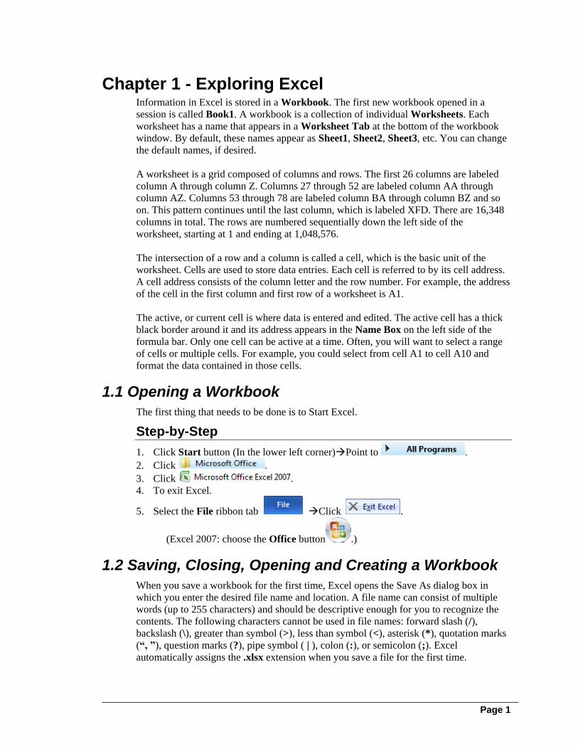
1.1 Opening a Workbook

The first thing that needs to be done is to Start Excel.

Step-by-Step

1. Click Start button (In the lower left corner)Point to .

2. Click .

3. Click .

4. To exit Excel.

5. Select the File ribbon tab Click .

(Excel 2007: choose the Office button .)

1.2 Saving, Closing, Opening and Creating a Workbook

When you save a workbook for the first time, Excel opens the Save As dialog box in

which you enter the desired file name and location. A file name can consist of multiple

words (up to 255 characters) and should be descriptive enough for you to recognize the

contents. The following characters cannot be used in file names: forward slash (/),

backslash (\), greater than symbol (>), less than symbol (<), asterisk (*), quotation marks

(“, ”), question marks (?), pipe symbol ( | ), colon (:), or semicolon (;). Excel

automatically assigns the .xlsx extension when you save a file for the first time.

Chapter 1 - Exploring Excel

Page 2

When you have finished working on a workbook, you can close it to remove it from the

application window.

When you start Excel, it opens with a new, blank workbook ready for you to work in.

Step-by-Step

1. Open a new workbook if necessary or continue from the previous exercise.

2. Select the File ribbon tab (Excel 2007: choose the Office button .)

3. Save File name: MyExcelClick .

4. Save the file in C:\DATAClick .

5. Select the File ribbon tab Click .

6. Select the File ribbon tab Click

7. Click Click

8. Click Click C:\DATAClick: MyExcel.xlsxClick.

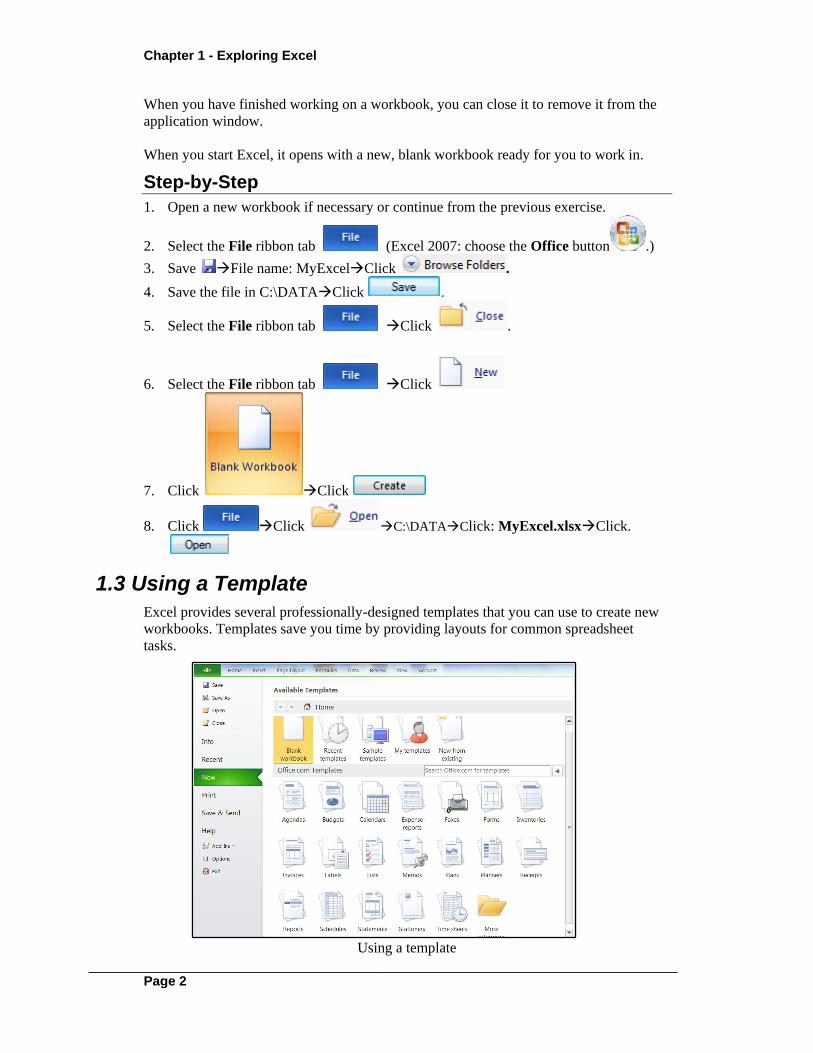
1.3 Using a Template

Excel provides several professionally-designed templates that you can use to create new

workbooks. Templates save you time by providing layouts for common spreadsheet

tasks.

Using a template

Excel 2010 - Fundamentals

Page 3

Step-by-Step

1. Select the File ribbon tab

2. Click Click Installed Templates.

3. Click Expense ReportClick

4. Close the ExpenseReport1 workbook without saving the changes.

1.4 The Ribbon

The Ribbon, located under the application title bar is a band of functional Tabs that

replaces the menu system used in previous versions. The Home ribbon tab brings

together the most frequently used commands in one easily accessible place. While some

buttons in the Ribbon immediately apply a command, such as the Bold button, other

buttons offer a large range of choices. When you see a button with a down-pointing

arrow, it indicates that the button offers several options. Generally, clicking this type of

button displays a Gallery, although some buttons display just a menu, while others show

both a gallery and a menu. A Gallery is a graphic display of the options available from

the button. If a button appears dimmed, it indicates that the command is not available for

the current task.

The buttons are arranged in named Groups within each tab. The Group Names appear

below the buttons. A Launcher Arrow to the right of some Group Names opens either a

dialog box or a task pane providing additional options not available from the buttons.

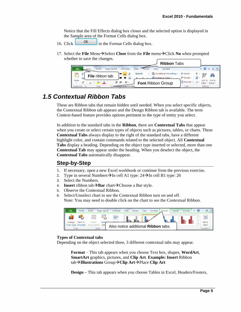
The Ribbon

Ribbon Tabs

The following are some of the ribbon tabs that appear on top of the ribbon:

File menu -This is located in the upper left corner and contains file related

commands.

Home ribbon tab - This contains most of the format-related concepts in one

ribbon.

Insert ribbon tab - Used to insert objects such as graphic items.

Page Layout ribbon tab – Used to define page settings or things that will affect

page layout.

Formulas ribbon tab - This includes the available formulas.


Page 4

Data ribbon tab – This includes data manipulation techniques.

Review ribbon tab - This includes spell check and tools that analyze the

document.

View ribbon tab - Includes Zoom, Print Layout, and window layout tools.

KeyTips – Press Alt key to display the KeyTips letter, use the arrows or press the letter

displayed to choose a command, and the Enter key to select the command.

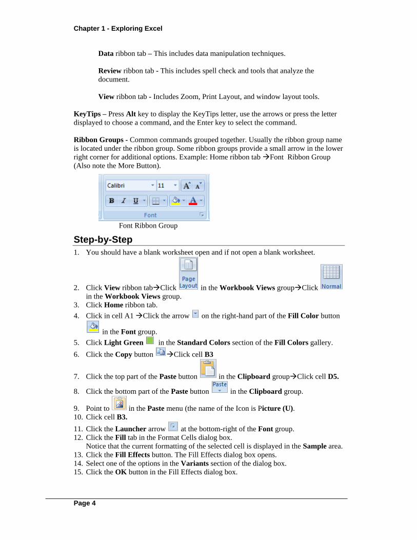
Ribbon Groups - Common commands grouped together. Usually the ribbon group name

is located under the ribbon group. Some ribbon groups provide a small arrow in the lower

right corner for additional options. Example: Home ribbon tab Font Ribbon Group

(Also note the More Button).

Font Ribbon Group

Step-by-Step

1. You should have a blank worksheet open and if not open a blank worksheet.

2. Click View ribbon tabClick in the Workbook Views groupClick

in the Workbook Views group.

3. Click Home ribbon tab.

4. Click in cell A1 Click the arrow on the right-hand part of the Fill Color button

in the Font group.

5. Click Light Green in the Standard Colors section of the Fill Colors gallery.

6. Click the Copy button Click cell B3

7. Click the top part of the Paste button in the Clipboard groupClick cell D5.

8. Click the bottom part of the Paste button in the Clipboard group.

9. Point to in the Paste menu (the name of the Icon is Picture (U).

10. Click cell B3.

11. Click the Launcher arrow at the bottom-right of the Font group.

12. Click the Fill tab in the Format Cells dialog box.

Notice that the current formatting of the selected cell is displayed in the Sample area.

13. Click the Fill Effects button. The Fill Effects dialog box opens.

14. Select one of the options in the Variants section of the dialog box.

15. Click the OK button in the Fill Effects dialog box.


Page 5

Notice that the Fill Effects dialog box closes and the selected option is displayed in

the Sample area of the Format Cells dialog box.

16. Click in the Format Cells dialog box.

17. Select the File MenuSelect Close from the File menuClick No when prompted

whether to save the changes.

1.5 Contextual Ribbon Tabs

These are Ribbon tabs that remain hidden until needed. When you select specific objects,

the Contextual Ribbon tab appears and the Design Ribbon tab is available. The term

Context-based feature provides options pertinent to the type of entity you select.

In addition to the standard tabs in the Ribbon, there are Contextual Tabs that appear

when you create or select certain types of objects such as pictures, tables, or charts. These

Contextual Tabs always display to the right of the standard tabs, have a different

highlight color, and contain commands related to the selected object. All Contextual

Tabs display a heading. Depending on the object type inserted or selected, more than one

Contextual Tab may appear under the heading. When you deselect the object, the

Contextual Tabs automatically disappear.

Step-by-Step

1. If necessary, open a new Excel workbook or continue from the previous exercise.

2. Type in several NumbersIn cell A1 type: 24In cell B1 type: 26

3. Select the Numbers.

4. Insert ribbon tabBar chartChoose a Bar style.

5. Observe the Contextual Ribbon.

6. Select/Unselect chart to see the Contextual Ribbon turn on and off.

Note: You may need to double click on the chart to see the Contextual Ribbon.

Types of Contextual tabs

Depending on the object selected three, 3 different contextual tabs may appear.

Format – This tab appears when you choose Text box, shapes, WordArt,

SmartArt graphics, pictures, and Clip Art. Example: Insert Ribbon

tabIllustrations GroupClip ArtPlace Clip Art

Design – This tab appears when you choose Tables in Excel, Headers/Footers,

Also notice additional Ribbon tabs.

Ribbon Tabs

Font Ribbon Group

File ribbon tab Button


Page 6

and SmartArt graphics. Example: Insert ribbon tabHeader & Footer

GroupHeaderBlank

Layout – This tab appears when you insert tables in Excel. Example: Insert

ribbon tabTable

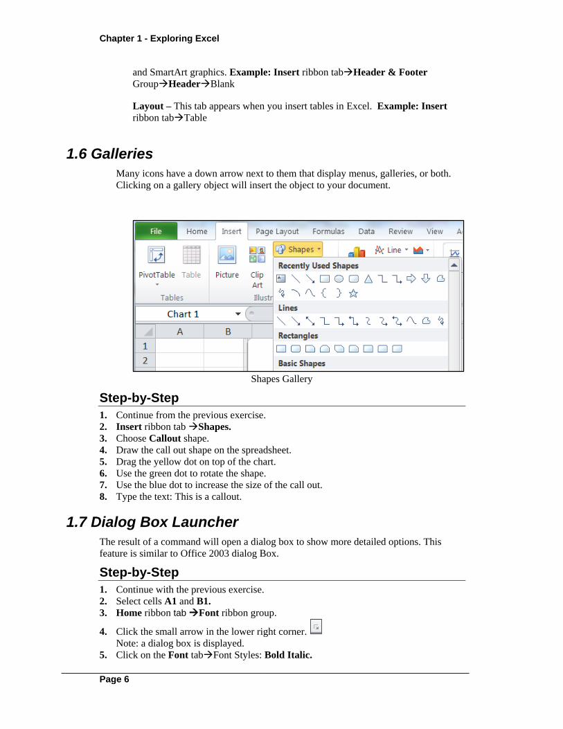
1.6 Galleries

Many icons have a down arrow next to them that display menus, galleries, or both.

Clicking on a gallery object will insert the object to your document.

Shapes Gallery

Step-by-Step

1. Continue from the previous exercise.

2. Insert ribbon tab Shapes.

3. Choose Callout shape.

4. Draw the call out shape on the spreadsheet.

5. Drag the yellow dot on top of the chart.

6. Use the green dot to rotate the shape.

7. Use the blue dot to increase the size of the call out.

8. Type the text: This is a callout.

1.7 Dialog Box Launcher

The result of a command will open a dialog box to show more detailed options. This

feature is similar to Office 2003 dialog Box.

Step-by-Step

1. Continue with the previous exercise.

2. Select cells A1 and B1.

3. Home ribbon tab Font ribbon group.

4. Click the small arrow in the lower right corner.

Note: a dialog box is displayed.

5. Click on the Font tabFont Styles: Bold Italic.


Page 7

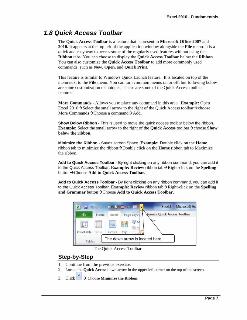
1.8 Quick Access Toolbar

The Quick Access Toolbar is a feature that is present in Microsoft Office 2007 and

2010. It appears at the top left of the application window alongside the File menu. It is a

quick and easy way to access some of the regularly used features without using the

Ribbon tabs. You can choose to display the Quick Access Toolbar below the Ribbon.

You can also customize the Quick Access Toolbar to add more commonly used

commands, such as New, Open, and Quick Print.

This feature is Similar to Windows Quick Launch feature. It is located on top of the

menu next to the File menu. You can turn common menus on or off, but following below

are some customization techniques. These are some of the Quick Access toolbar

features:

More Commands - Allows you to place any command in this area. Example: Open

Excel 2010Select the small arrow to the right of the Quick Access toolbarchoose

More CommandsChoose a commandAdd.

Show Below Ribbon - This is used to move the quick access toolbar below the ribbon.

Example: Select the small arrow to the right of the Quick Access toolbarchoose Show

below the ribbon.

Minimize the Ribbon - Saves screen Space. Example: Double click on the Home

ribbon tab to minimize the ribbonDouble click on the Home ribbon tab to Maximize

the ribbon. Add to Quick Access Toolbar - By right clicking on any ribbon command, you can add it

to the Quick Access Toolbar. Example: Review ribbon tabRight-click on the Spelling

buttonChoose Add to Quick Access Toolbar. Add to Quick Access Toolbar - By right clicking on any ribbon command, you can add it

to the Quick Access Toolbar. Example: Review ribbon tabRight-click on the Spelling

and Grammar buttonChoose Add to Quick Access Toolbar.

The Quick Access Toolbar

Step-by-Step


2. Locate the Quick Access down arrow in the upper left corner on the top of the screen.

3. Click

Choose Minimize the Ribbon.

The down arrow is located here.


Page 8

4. Click

Choose Maximize the Ribbon (note: you can also double click on the Home

ribbon tab.

5. Click

6. Click Open (make sure there is a check mark in front of open).

Notice the Open icon is now added to the Quick Launch toolbar.

7. Click

Located in the upper left corner on the top of the screen.

8. Click More CommandsClick All Commands.

Review the many commands available.

9. Click the “5-Point Star” AddClick

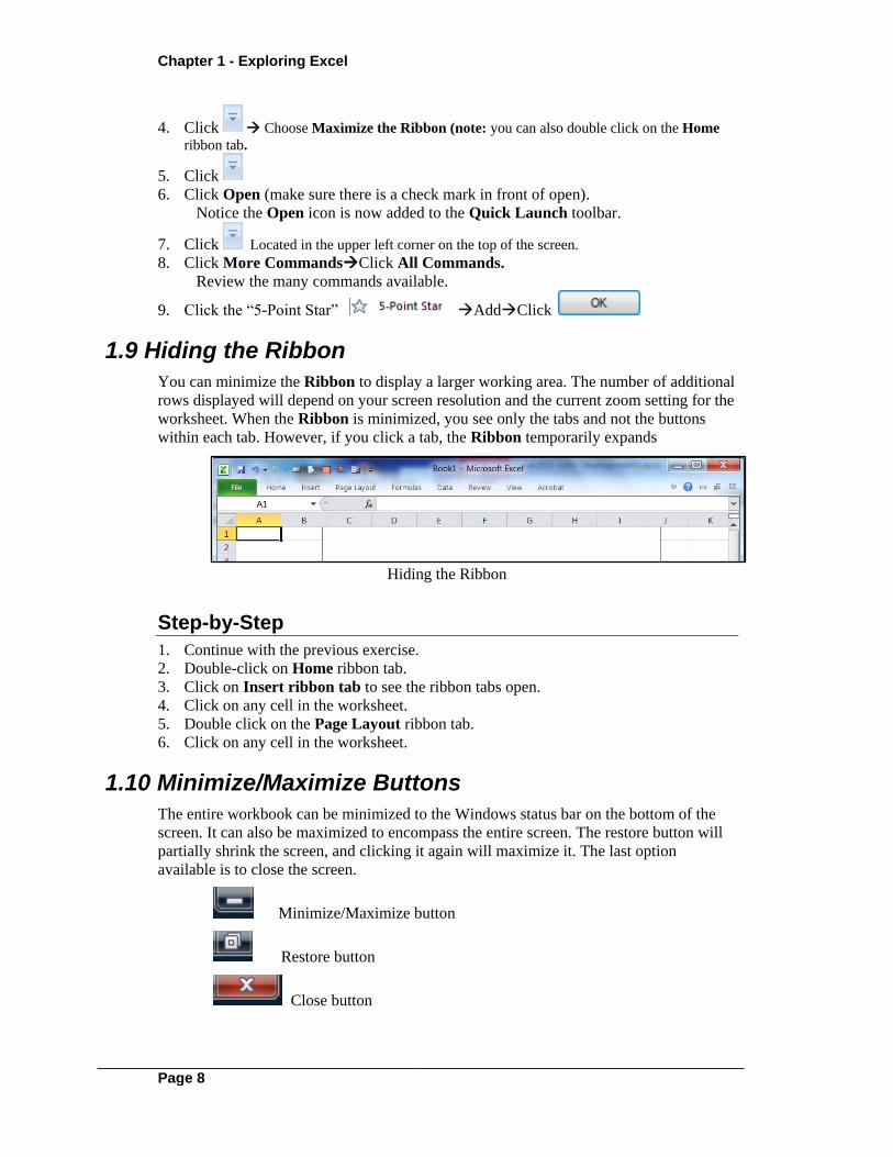
1.9 Hiding the Ribbon

You can minimize the Ribbon to display a larger working area. The number of additional

rows displayed will depend on your screen resolution and the current zoom setting for the

worksheet. When the Ribbon is minimized, you see only the tabs and not the buttons

within each tab. However, if you click a tab, the Ribbon temporarily expands

Hiding the Ribbon

Step-by-Step


2. Double-click on Home ribbon tab.

3. Click on Insert ribbon tab to see the ribbon tabs open.

4. Click on any cell in the worksheet.

5. Double click on the Page Layout ribbon tab.

6. Click on any cell in the worksheet.

1.10 Minimize/Maximize Buttons

The entire workbook can be minimized to the Windows status bar on the bottom of the

screen. It can also be maximized to encompass the entire screen. The restore button will

partially shrink the screen, and clicking it again will maximize it. The last option

available is to close the screen.

Minimize/Maximize button

Restore button

Close button


Page 9

Step-by-Step


2. Click on the Minimize button.

3. Click on the Excel workbook on the bottom of the screen to maximize Excel.

4. Click on the restore button.

5. Click on the restore button again to maximize the workbook.

6. Click on the close button to close the workbook.

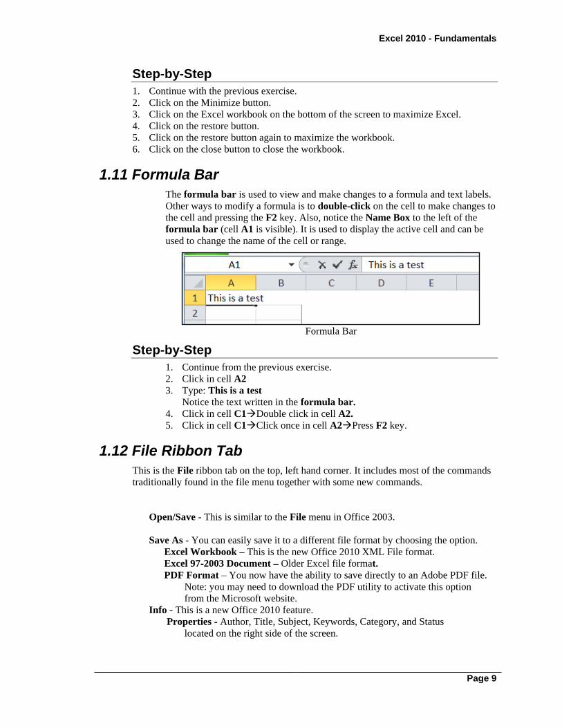
1.11 Formula Bar

The formula bar is used to view and make changes to a formula and text labels.

Other ways to modify a formula is to double-click on the cell to make changes to

the cell and pressing the F2 key. Also, notice the Name Box to the left of the

formula bar (cell A1 is visible). It is used to display the active cell and can be

used to change the name of the cell or range.

Formula Bar

Step-by-Step


2. Click in cell A2

3. Type: This is a test

Notice the text written in the formula bar.

4. Click in cell C1Double click in cell A2.

5. Click in cell C1Click once in cell A2Press F2 key.

1.12 File Ribbon Tab

This is the File ribbon tab on the top, left hand corner. It includes most of the commands

traditionally found in the file menu together with some new commands.

Open/Save - This is similar to the File menu in Office 2003.

Save As - You can easily save it to a different file format by choosing the option.

Excel Workbook – This is the new Office 2010 XML File format.

Excel 97-2003 Document – Older Excel file format.

PDF Format – You now have the ability to save directly to an Adobe PDF file.

Note: you may need to download the PDF utility to activate this option

from the Microsoft website.

Info - This is a new Office 2010 feature.

Properties - Author, Title, Subject, Keywords, Category, and Status

located on the right side of the screen.


Page 10

Protect Workbook – Provide Workbook Protection such as

Mark as final which the file will become read only and all

formatting and modification tools are disabled.

Check for Issues – One feature is the Inspect Document which inspects

document for hidden metadata, personal information, Custom XML

code, information in headers, footers, watermarks, and formatted

hidden text.

Manage Versions – This will recover old versions of the document.

Recent - Displays the previous opened files.

New - You can now quickly preview the available online templates.

Print – Many printing options are now available.

Save/Send – Will send the document through email.

Step-by-Step


2. Select the File ribbon tab PrepareMark as FinalOK.

3. The following menu appears when you mark a document as final:

4. Select the File ribbon tab PrepareMark as Final (to unmark the

document as final).

5. Select the File ribbon tab OpenClick once on a file: MyExcel.xlsx.

6. Hold cursor over a file to view properties. The result will look similar to the

following:

7. Cancel the open dialog box.

8. To update Properties choose the File ribbon tab PrepareProperties.

9. Type in a title of: My Spreadsheet

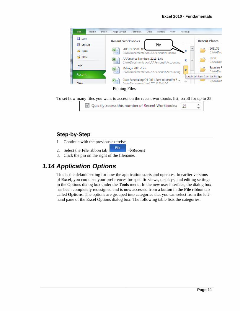
1.13 Pinning Files

This is used to Pin the files you need to reopen in the future such as Status Reports,

Timesheet Spreadsheets, etc.


Page 11

Pinning Files

To set how many files you want to access on the recent workbooks list, scroll for up to 25

Step-by-Step


2. Select the File ribbon tab Recent

3. Click the pin on the right of the filename.

1.14 Application Options

This is the default setting for how the application starts and operates. In earlier versions

of Excel, you could set your preferences for specific views, displays, and editing settings

in the Options dialog box under the Tools menu. In the new user interface, the dialog box

has been completely redesigned and is now accessed from a button in the File ribbon tab

called Options. The options are grouped into categories that you can select from the left-

hand pane of the Excel Options dialog box. The following table lists the categories:

Pin


Page 12

Excel Options

Popular Excel Option

X Show Mini Toolbar on selection - Shows the Mini Toolbar popup when you

select text. The Mini Toolbar provides quick access to formatting tools. The mini

toolbar is context-based in that it provides options based on the type of selection

you choose. In Excel, you need to select the actual text, not just the cell.

X Enable Live Preview - The live preview shows the selected text as an example of

what can be chosen as you look over the various font type options.

Color Scheme - The menu color scheme options are Blue. Silver, and Black.

ScreenTip style - Select a style from the list to control the display of the names of

buttons and additional helpful information.

User name - Type a name in the User name box to change the value.


Page 13

Step-by-Step


2. Choose one of the options belowHold cursor over any menu item.

Show feature descriptions in ScreenTips - Display ScreenTip names

and information. The ScreenTip looks like the following:

Don't show feature descriptions in ScreenTips - Display ScreenTip button

names only. The ScreenTip looks like the following:

Don't show ScreenTips - Disables the ScreenTip from displaying.

Note: Display a Screen Tip and press F1 to get help on that specific item.

Formulas Excel Option - Change options related to formula calculation,

performance, and error handling.

Proofing Excel Option - Change how Excel corrects and formats your text.

Save Excel Option -Customize how workbooks are saved.

Advanced Excel Option = This category includes, among others, sections for

Editing, Cut, copy and paste, Print, Display (including options for currently

open workbooks and individual worksheets), Calculation in currently open

workbooks and General options.

Customize Excel Option - Customize the Quick Access Toolbar (including the

ability to add commands not available in the Ribbon).

Add-Ins Excel Option - View and manage Microsoft Office add-ins.

Trust Center Excel Option - Help keep your documents safe and your computer

secure and healthy (Privacy and Security options).

Resources Excel Option - Contact Microsoft, find on-line resources, and

maintain health and reliability of your Microsoft Office programs (includes

options to check for updates to Microsoft Office and to diagnose and repair

problems with Microsoft Office programs).

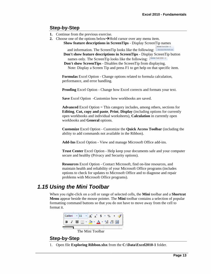
1.15 Using the Mini Toolbar

When you right-click on a cell or range of selected cells, the Mini toolbar and a Shortcut

Menu appear beside the mouse pointer. The Mini toolbar contains a selection of popular

formatting command buttons so that you do not have to move away from the cell to

format it.

The Mini Toolbar

Step-by-Step

1. Open file Exploring Ribbon.xlsx from the C:\Data\Excel2010-1 folder.


Page 14

2. Right-click cell A1.

3. Click the Bold button in the Mini toolbar.

4. Click the Team Sales heading in the chart.

Drag to select the words Team Sales.

5. Move the mouse pointer over the Mini toolbar.

6. Click the Increase Font Size button in the Mini toolbar.

7. Select the Team Leader text in the text box. Italicize the text using the Mini

Toolbar.

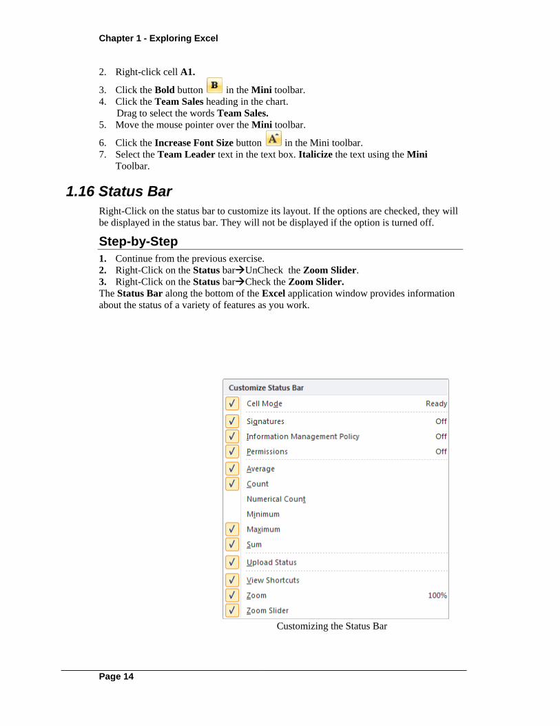
1.16 Status Bar

Right-Click on the status bar to customize its layout. If the options are checked, they will

be displayed in the status bar. They will not be displayed if the option is turned off.

Step-by-Step


2. Right-Click on the Status barUnCheck the Zoom Slider.

3. Right-Click on the Status barCheck the Zoom Slider.

The Status Bar along the bottom of the Excel application window provides information

about the status of a variety of features as you work.

Customizing the Status Bar


Page 15

Practice1 Exercise - Exploring Excel

1. Start Excel, if necessary and open a blank worksheet.

2. Display the File menu.

3. Open the Excel Options dialog box.

4. Under the Display options for this worksheet section in the

Advanced category, change the Gridline color to Yellow,

then select OK.

5. View the color change to the worksheet gridlines.

6. Change the Gridline color back to Automatic.

7. Minimize the Ribbon.

8. Select cell C5.

9. Use the Fill Color button on the Home ribbon tab to set the

color of cell C5 to Yellow.

10. Customize the Quick Access Toolbar by adding the Quick

Print command icon.

11. Remove the Quick Print command from the Quick Access

Toolbar.

12. Right-click cell C5 and use the Mini toolbar to set the Fill

Color of the cell to No Fill.

13. Maximize the Ribbon.

14. Exit Excel without saving changes to the workbook.

Chapter 2 – Navigation Techniques

You can use the Mouse or Keyboard to move around in Excel. The scrollbar on the right

and on the bottom is very useful, but the most common method is dragging the mouse in

the worksheet to the edge of the window. The ability to zoom the sheet to see more

information and inspecting cells closer is useful. This chapter will discuss the techniques

to accomplish this objective.

2.1 Keyboard Commands

You can use the keyboard to navigate within Excel. When you press certain arrow keys

or a combination of keys, the cell pointer moves to a new cell, making it the active cell.

This will move the screen depending on the direction of the keyboard command.

Step-by-Step

1. Open the file Navigation.xlsx in the folder C:\Data\Excel2010-1.

2. Press key to move one cell down.

3. Press key to move one cell to the right.

4. Press key to move one cell up.

5. Press key to move one cell to the left.

6. Press Page Down to move down one screen.

7. Press Alt+Page Down keys to move one screen to the right.

8. Press Page Up key to move up one screen.

9. Press Alt+Page Up key to move one screen to the left.

10. Press Ctrl+Home keys to move to the upper, left cell in the worksheet.

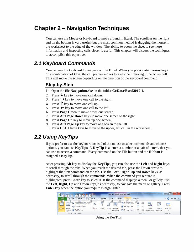
2.2 Using KeyTips

If you prefer to use the keyboard instead of the mouse to select commands and choose

options, you can use KeyTips. A KeyTip is a letter, a number or a pair of letters, that you

can use to access a command. Every command on the File button and the Ribbon is

assigned a KeyTip.

After pressing Alt key to display the KeyTips, you can also use the Left and Right keys

to scroll through the tabs. When you reach the desired tab, press the Down arrow to

highlight the first command on the tab. Use the Left, Right, Up and Down keys, as

necessary, to scroll through the commands. When the command you require is

highlighted, press Enter key to select it. If the command displays a menu or gallery, use

the Left, Right, Up and Down keys, as necessary, to navigate the menu or gallery. Press

Enter key when the option you require is highlighted.

Using the KeyTips

Page 18

Step-by-Step


2. Press Alt key

3. Press H key

4. Press H key

5. Press the Right key five times to highlight Red, Accent 2 (sixth color, first row)

6. Press Enter key

2.3 Using the Mouse on the Scroll Bar

You can use the mouse to select a different cell as the active cell. However, if the cell you

wish to select is not currently visible you must first scroll the screen display to bring it

into view. On larger worksheets, all the data may not fit on the screen display at once.

The horizontal and vertical scroll bars allow you to scroll the display so that you can view

other parts of the worksheet.

There are three elements on a scroll bar that you can use to scroll the worksheet:

Scroll Arrows at the top and bottom of the vertical scroll bar and at the left and

right ends of the horizontal scroll bar scroll the worksheet up and down or left

and right one row or column at a time with each click of the mouse on the

relevant arrow.

You can drag the Scroll Box (the gray rectangle on the scroll bar with 4 lines in

the middle) up and down or left and right, as appropriate, to scroll quickly within

the area of the worksheet that you have utilized so far.

Scroll Arrow to scroll up, down, left or right one screen page at a time.

Vertical Scroll bar.

Horizontal Scroll bar.

Horizontal Scroll box.

Area between the Scroll

box and down arrow.


Excel Networks Page 19

Step-by-Step

1. Continue using the previous exercise.

2. Click cell D7.

3. Click the Down Arrow at the bottom of the vertical scroll bar 3 times.

4. Click the Right Arrow at the right-hand end of the horizontal scroll bar 3 times.

5. Drag the horizontal Scroll Box to the left end of the scroll bar.

6. Click the space between the Scroll Box and the Down Arrow in the vertical scroll

bar.

7. Hold down the Shift key and drag the horizontal Scroll Box halfway along

the scroll bar.

8. Press Ctrl+Home keys.

9. Press Page Down key two times to scroll down two screens and reposition the active

cell.

10. Drag the Scroll Box to the top of the vertical scroll bar.

Notice that the display scrolls to row 1.

Notice that the Name Box to the left of the formula bar shows that the active cell has

not changed position. Click cell A1 to select it. Notice that the Name Box now shows

A1.

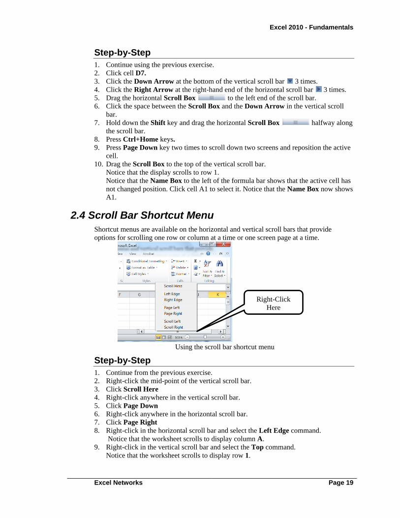
2.4 Scroll Bar Shortcut Menu

Shortcut menus are available on the horizontal and vertical scroll bars that provide

options for scrolling one row or column at a time or one screen page at a time.

Using the scroll bar shortcut menu

Step-by-Step


2. Right-click the mid-point of the vertical scroll bar.

3. Click Scroll Here

4. Right-click anywhere in the vertical scroll bar.

5. Click Page Down

6. Right-click anywhere in the horizontal scroll bar.

7. Click Page Right

8. Right-click in the horizontal scroll bar and select the Left Edge command.

Notice that the worksheet scrolls to display column A.

9. Right-click in the vertical scroll bar and select the Top command.

Notice that the worksheet scrolls to display row 1.

Right-Click

Here

Page 20

2.5 Mouse Drag

Using the mouse you can click on any cell. Hold the left mouse button down and drag to

the edge of the page. You can adjust the speed of scrolling by moving the selected area

off the page. This will be the commonly used command because as you are typing, you

may run out of room and dragging the cursor to the right or bottom will let you type

additional information.

Step-by-Step


2. Click anywhere in the middle of the worksheet.

3. Hold the left mouse button down and drag to the bottom of the window.

4. When the cells begin to move push the cursor further down to see the screen move

faster.

5. Click anywhere in the middle of the worksheet.

6. Hold the left mouse button down and drag to the right of the window.

7. When the cells begin to move push the cursor further down to see the screen move

faster.

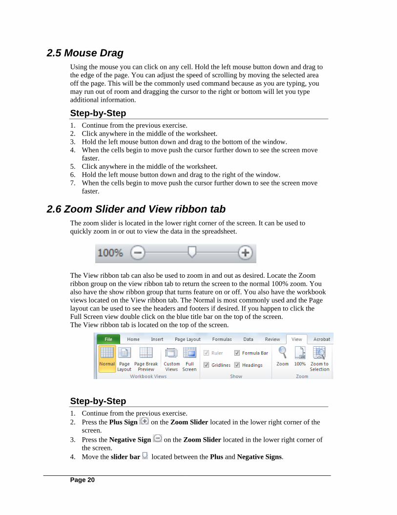
2.6 Zoom Slider and View ribbon tab

The zoom slider is located in the lower right corner of the screen. It can be used to

quickly zoom in or out to view the data in the spreadsheet.

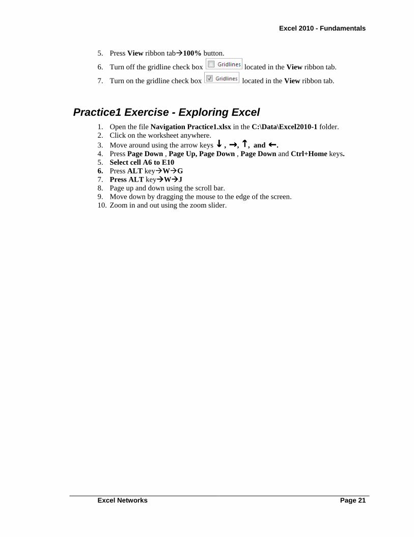
The View ribbon tab can also be used to zoom in and out as desired. Locate the Zoom

ribbon group on the view ribbon tab to return the screen to the normal 100% zoom. You

also have the show ribbon group that turns feature on or off. You also have the workbook

views located on the View ribbon tab. The Normal is most commonly used and the Page

layout can be used to see the headers and footers if desired. If you happen to click the

Full Screen view double click on the blue title bar on the top of the screen.

The View ribbon tab is located on the top of the screen.

Step-by-Step


2. Press the Plus Sign on the Zoom Slider located in the lower right corner of the

screen.

3. Press the Negative Sign on the Zoom Slider located in the lower right corner of

the screen.

4. Move the slider bar located between the Plus and Negative Signs.


Excel Networks Page 21

5. Press View ribbon tab100% button.

6. Turn off the gridline check box located in the View ribbon tab.

7. Turn on the gridline check box located in the View ribbon tab.

Practice1 Exercise - Exploring Excel

1. Open the file Navigation Practice1.xlsx in the C:\Data\Excel2010-1 folder.

2. Click on the worksheet anywhere.

3. Move around using the arrow keys , , , and .

4. Press Page Down , Page Up, Page Down , Page Down and Ctrl+Home keys.

5. Select cell A6 to E10

6. Press ALT keyWG

7. Press ALT keyWJ

8. Page up and down using the scroll bar.

9. Move down by dragging the mouse to the edge of the screen.

10. Zoom in and out using the zoom slider.

Documents

Microsoft Excel 2010 - Dashboard