Microsoft Excel 2013 Only Lesson 1: Introducing …ccilearning.com/store-ca/wp-content/uploads/2014/10/6280-1-Excel...Microsoft® Excel 2013 ... Excel uses the term worksheet in place

6280-1 v1.00 © CCI Learning Solutions Inc. 1

Microsoft®

Excel 2013

Lesson 1: Introducing Excel

Lesson Objectives The objectives of this lesson are to introduce the Excel program, learn how it works, and understand how to move in the program, create a workbook, enter data into a worksheet, and work with files. Upon completion of this lesson, you should be able to:

understand what an electronic spreadsheet is

understand what Excel is and what it can do

identify elements on the Excel screen

understand some basic terminology

use the Quick Access Toolbar

move around in Excel

use keyboard shortcuts

enter text, numbers, dates, and times

move around a worksheet

use the Office Backstage View to save, create new, open, and close a workbook

switch between workbooks

save in a previous version Excel format

manage files and folders

select cells

What is Excel? Excel is an electronic spreadsheet program developed by Microsoft for the Windows environment. A powerful tool for analyzing and presenting information, Excel actually consists of three programs in one:

Spreadsheet Entering and analyzing data such as financial forecasting, cash flow, and auditing. Excel uses the term worksheet in place of spreadsheet.

Graphics Creating charts to represent numeric data.

Database Compiling and sorting lists.

For E

valua

tion O

nly

Lesson 1 Viewing and Printing Workbooks

2 6280-1 v1.00 © CCI Learning Solutions Inc.

Some of Excel’s advantages are:

It is relatively easy to learn. All Windows programs, such as Word, Excel, and PowerPoint, operate similarly. Many of the skills you learn in one Windows program carry over to others.

Windows allows an exchange of data between programs. For example, you can create a chart in Excel and insert it into a memo you are writing in Word.

Excel can produce output of print-shop quality using features such as the spelling checker and other tools that enhance your work and provide it with a professional look.

Excel has a large selection of mathematical, financial, statistical, and database functions. It includes 10 basic chart types and each chart type has three or more subtypes. There are also some tools for forecasting or analysis, and a function helper.

Worksheets can be grouped together in a single file rather than separate files. In Excel, these files are called workbooks. Inside a workbook, there are several ways to manage the multiple worksheets such as renaming worksheet tabs.

Excel uses AutoFill to fill selected cells with data that follows from the information in the first of the selected cells. For example, if you select four cells, and the first cell contains Qtr 1, AutoFill will fill in the next three cells with Qtr 2, Qtr 3, and Qtr 4.

By default, edits occur directly in the cell. This includes formatting portions of text and making font changes. Alternatively, you can perform edits in the formula bar.

Although Excel is a very large program, it is enjoyable to learn and use. Most people find it takes them less time to become competent and productive with Excel than they initially anticipated.

Starting the Microsoft Excel Program In Windows 8, there are several ways to start the Excel program:

From the Start screen, click or tap the Excel 2013 tile. You will then switch to the Desktop, where Excel runs.

From the All Apps screen, click or tap the Excel 2013 icon. You will then switch to the Desktop, where Excel runs.

In the Desktop, click the Excel 2013 Quick Launch icon in the taskbar.

In Windows 7 and earlier versions of Windows, Excel can be launched in several ways on the Desktop:

Click the Windows Start button, then select All Programs, Microsoft Office 2013, Excel 2013.

If available, double-click the Microsoft Excel shortcut on the Windows Desktop.

If available, click the Microsoft Excel Quick Launch icon in the taskbar.

Excel will only run on the Desktop for all versions of Windows including Windows 8.

For E

valua

tion O

nly

Viewing and Printing Workbooks Lesson 1


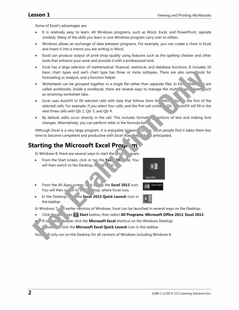
Looking at the Screen When Excel starts, a new workbook opens and the screen displays as follows:

File Tab When clicked, this displays the Office Backstage View from which you can select commands for a file (for example, Save, Open, and Close). A panel at the left displays commands that may include tabs with a set of sub-commands to manage the file.

Quick Access Toolbar

Located above the Ribbon, this provides quick access to frequently used commands. You can customize the toolbar to contain commands you use regularly.

Title Bar Located at the top of the screen, the title bar indicates the contents of the window (for example, Book1, Department Budget - Excel). It may also show the text [Compatibility Mode] if the workbook you are using has been saved to be compatible with a previous version of Excel. If more than one window is open on the screen, the one with a title bar that has a darker color or intensity is the active window.

Microsoft Office Excel Help

Displays the Help window to obtain the latest help on a feature. Microsoft’s Help option links to the Microsoft Web site for the latest information. Alternatively, you can also use the Help topics installed with Office.

Minimize, Maximize, Restore, Close the Window

Located in the upper right-hand corner of the window, these buttons enable you to minimize ( ) the application window to a button on the taskbar, maximize ( ) the program to full screen, restore ( ) the window to its original size, or close ( ) the application window.

Close File Quick Access Ribbon Title Maximize/Restore Tab Toolbar Bar Minimize

Name Box Insert Function Formula Bar Help Ribbon Column Display Headings Options

Active Cell

Row Headings

Tab Sheet Status Bar View Buttons Zoom SliderScrolling Tab Buttons

Scroll Bars

For E

valua

tion O

nly



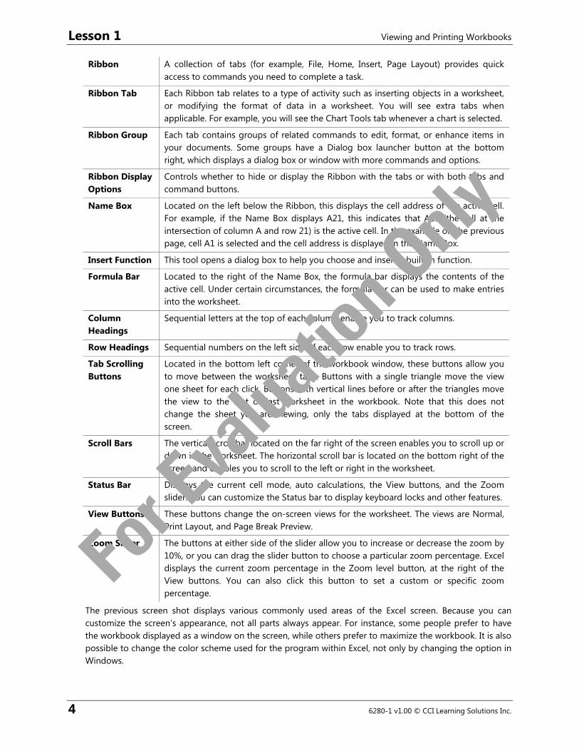
Ribbon A collection of tabs (for example, File, Home, Insert, Page Layout) provides quick access to commands you need to complete a task.

Ribbon Tab Each Ribbon tab relates to a type of activity such as inserting objects in a worksheet, or modifying the format of data in a worksheet. You will see extra tabs when applicable. For example, you will see the Chart Tools tab whenever a chart is selected.

Ribbon Group Each tab contains groups of related commands to edit, format, or enhance items in your documents. Some groups have a Dialog box launcher button at the bottom right, which displays a dialog box or window with more commands and options.

Ribbon Display Options

Controls whether to hide or display the Ribbon with the tabs or with both tabs and command buttons.

Name Box Located on the left below the Ribbon, this displays the cell address of the active cell. For example, if the Name Box displays A21, this indicates that A21 (the cell at the intersection of column A and row 21) is the active cell. In the example on the previous page, cell A1 is selected and the cell address is displayed in the Name Box.

Insert Function This tool opens a dialog box to help you choose and insert a built-in function.

Formula Bar Located to the right of the Name Box, the formula bar displays the contents of the active cell. Under certain circumstances, the formula bar can be used to make entries into the worksheet.

Column Headings

Sequential letters at the top of each column enable you to track columns.

Row Headings Sequential numbers on the left side of each row enable you to track rows.

Tab Scrolling Buttons

Located in the bottom left corner of the workbook window, these buttons allow you to move between the worksheet tabs. Buttons with a single triangle move the view one sheet for each click. Buttons with vertical lines before or after the triangles move the view to the first or last worksheet in the workbook. Note that this does not change the sheet you are viewing, only the tabs displayed at the bottom of the screen.

Scroll Bars The vertical scroll bar located on the far right of the screen enables you to scroll up or down in the worksheet. The horizontal scroll bar is located on the bottom right of the screen and enables you to scroll to the left or right in the worksheet.

Status Bar Displays the current cell mode, auto calculations, the View buttons, and the Zoom slider. You can customize the Status bar to display keyboard locks and other features.

View Buttons These buttons change the on-screen views for the worksheet. The views are Normal, Print Layout, and Page Break Preview.

Zoom Slider The buttons at either side of the slider allow you to increase or decrease the zoom by 10%, or you can drag the slider button to choose a particular zoom percentage. Excel displays the current zoom percentage in the Zoom level button, at the right of the View buttons. You can also click this button to set a custom or specific zoom percentage.

The previous screen shot displays various commonly used areas of the Excel screen. Because you can customize the screen’s appearance, not all parts always appear. For instance, some people prefer to have the workbook displayed as a window on the screen, while others prefer to maximize the workbook. It is also possible to change the color scheme used for the program within Excel, not only by changing the option in Windows.

For E

valua

tion O

nly



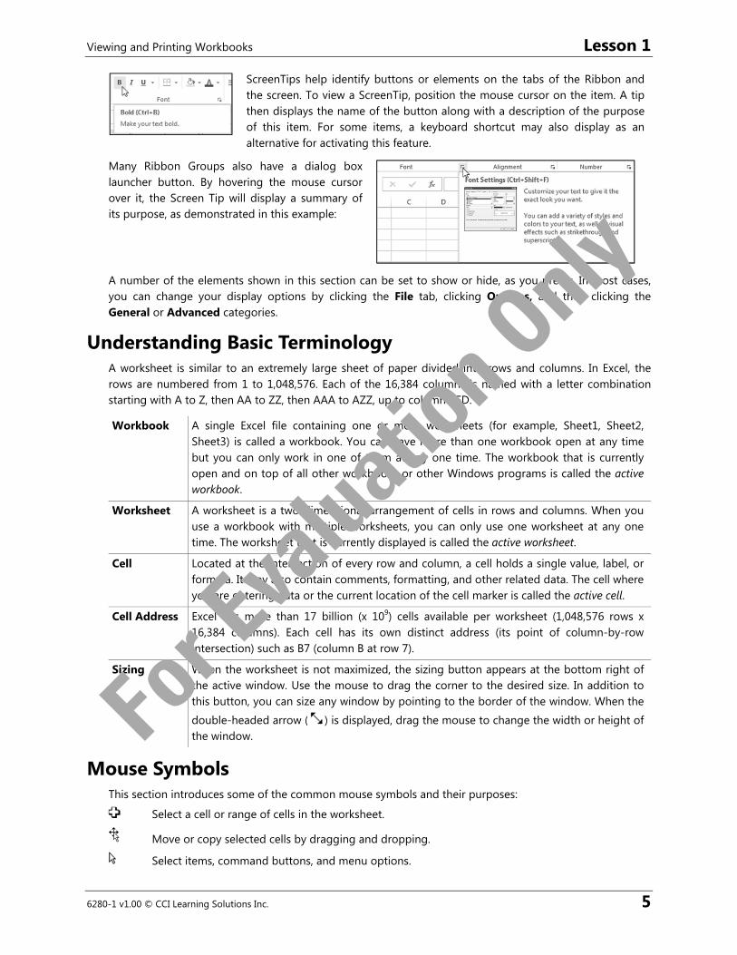
ScreenTips help identify buttons or elements on the tabs of the Ribbon and the screen. To view a ScreenTip, position the mouse cursor on the item. A tip then displays the name of the button along with a description of the purpose of this item. For some items, a keyboard shortcut may also display as an alternative for activating this feature.

Many Ribbon Groups also have a dialog box launcher button. By hovering the mouse cursor over it, the Screen Tip will display a summary of its purpose, as demonstrated in this example:

A number of the elements shown in this section can be set to show or hide, as you prefer. In most cases, you can change your display options by clicking the File tab, clicking Options, and then clicking the General or Advanced categories.

Understanding Basic Terminology A worksheet is similar to an extremely large sheet of paper divided into rows and columns. In Excel, the rows are numbered from 1 to 1,048,576. Each of the 16,384 columns is named with a letter combination starting with A to Z, then AA to ZZ, then AAA to AZZ, up to column XFD.

Workbook A single Excel file containing one or more worksheets (for example, Sheet1, Sheet2, Sheet3) is called a workbook. You can have more than one workbook open at any time but you can only work in one of them at any one time. The workbook that is currently open and on top of all other workbooks or other Windows programs is called the active workbook.

Worksheet A worksheet is a two-dimensional arrangement of cells in rows and columns. When you use a workbook with multiple worksheets, you can only use one worksheet at any one time. The worksheet that is currently displayed is called the active worksheet.

Cell Located at the intersection of every row and column, a cell holds a single value, label, or formula. It may also contain comments, formatting, and other related data. The cell where you are entering data or the current location of the cell marker is called the active cell.

Cell Address Excel has more than 17 billion (x 109) cells available per worksheet (1,048,576 rows x 16,384 columns). Each cell has its own distinct address (its point of column-by-row intersection) such as B7 (column B at row 7).

Sizing When the worksheet is not maximized, the sizing button appears at the bottom right of the active window. Use the mouse to drag the corner to the desired size. In addition to this button, you can size any window by pointing to the border of the window. When the

double-headed arrow ( ) is displayed, drag the mouse to change the width or height of the window.

Mouse Symbols This section introduces some of the common mouse symbols and their purposes:

Select a cell or range of cells in the worksheet.

Move or copy selected cells by dragging and dropping.

Select items, command buttons, and menu options.

For E

valua

tion O

nly



Size objects.

Edit text within the formula bar or a cell.

Indicates the use of the AutoFill feature to copy the contents of cells.

Provides a guide for the top left and bottom right corners when creating objects.

Change the column width or row height.

Move the split bar between the window panes.

Select an entire row or entire column.

It is possible to use Excel with a touchscreen, however, you will find it is generally easier to use a mouse and keyboard.

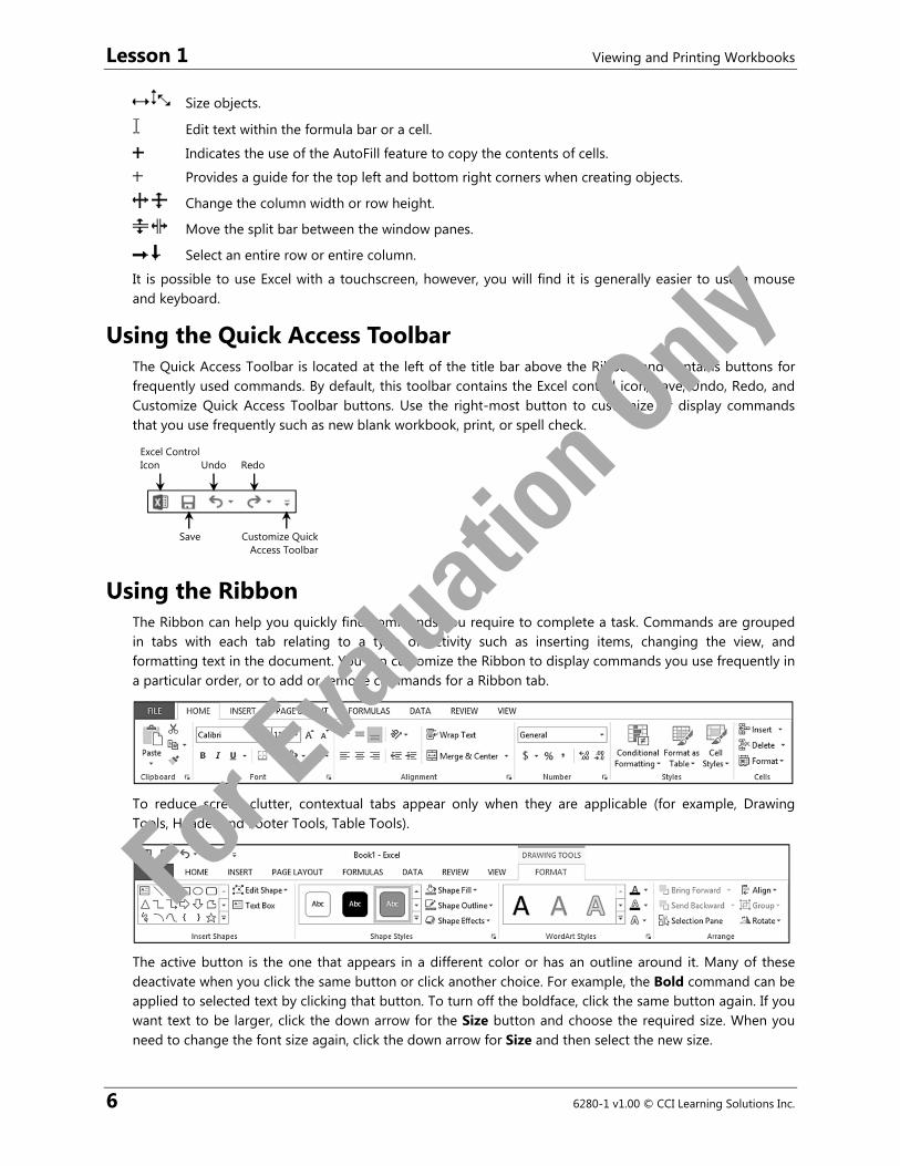
Using the Quick Access Toolbar The Quick Access Toolbar is located at the left of the title bar above the Ribbon and contains buttons for frequently used commands. By default, this toolbar contains the Excel control icon, Save, Undo, Redo, and Customize Quick Access Toolbar buttons. Use the right-most button to customize or display commands that you use frequently such as new blank workbook, print, or spell check.

Using the Ribbon The Ribbon can help you quickly find commands you require to complete a task. Commands are grouped in tabs with each tab relating to a type of activity such as inserting items, changing the view, and formatting text in the document. You can customize the Ribbon to display commands you use frequently in a particular order, or to add or remove commands for a Ribbon tab.

To reduce screen clutter, contextual tabs appear only when they are applicable (for example, Drawing Tools, Header and Footer Tools, Table Tools).

The active button is the one that appears in a different color or has an outline around it. Many of these deactivate when you click the same button or click another choice. For example, the Bold command can be applied to selected text by clicking that button. To turn off the boldface, click the same button again. If you want text to be larger, click the down arrow for the Size button and choose the required size. When you need to change the font size again, click the down arrow for Size and then select the new size.

Excel Control Icon Undo Redo

Save Customize Quick Access Toolbar

For E

valua

tion O

nly



When the Ribbon displays different choices (as shown in the Shape Styles list in the screen above), one item has a border around it to indicate it is active. To see how the text would appear with another style, point the mouse on one of the other items. Excel previews the effect that will take place if it is selected.

Each tab on the Ribbon contains groups with similar commands. For example, the Home tab has a group called Font that contains buttons for formatting text characters, and the Insert tab contains a group with different types of graphics or illustrations that can be inserted into a worksheet.

If a group shows a feature with a vertical scroll bar, it also has a button below the bottom scroll button, a triangle with a bar above it, which you can click to display the full list or gallery for that option.

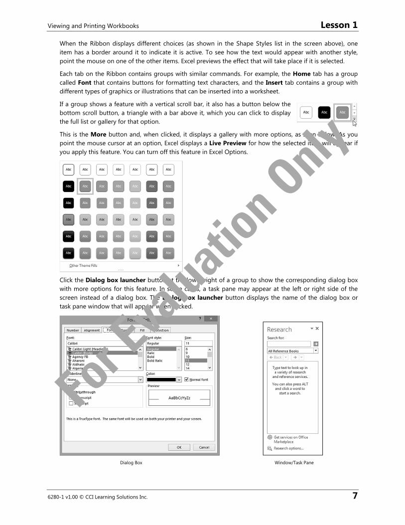
This is the More button and, when clicked, it displays a gallery with more options, as seen below. As you point the mouse cursor at an option, Excel displays a Live Preview for how the selected item will appear if you apply this feature. You can turn off this feature in Excel Options.

Click the Dialog box launcher button at the lower right of a group to show the corresponding dialog box with more options for this feature. In some cases, a task pane may appear at the left or right side of the screen instead of a dialog box. The Dialog box launcher button displays the name of the dialog box or task pane window that will appear when clicked.

Dialog Box Window/Task Pane

For E

valua

tion O

nly



Within the dialog box, you can select items from the lists, use the arrow for a list box to display more choices for that list, or click a command to turn the feature on or off. It may display a preview of the changes.

A dialog box displays the various options that you can select to perform a change to a worksheet or cells within a worksheet. Once you click OK to perform the change, the dialog box closes. A task pane is similar to a dialog box because it is used to make changes to parts of the worksheet, except that it remains open until you close it. An example of a task pane is the Office Clipboard which collects and displays the items selected when the Cut or Copy command is used.

If you want to show more lines on the screen or you do not want to display the Ribbon, you can minimize it. To minimize the Ribbon, use one of the following methods:

Point at the button at the upper right of the screen, then click Show Tabs, or

right-click anywhere on the Ribbon and then click Collapse the Ribbon, or

double-click on any Ribbon tab, or

press + .

Using the Keyboard You can also access commands in Excel using the keyboard. Some users consider the keyboard to be a faster method for accessing commands. There is also the benefit of consistency between Windows programs, in that many keyboard shortcuts are the same in all Windows programs such as pressing

+ to copy, + to save, or + to print.

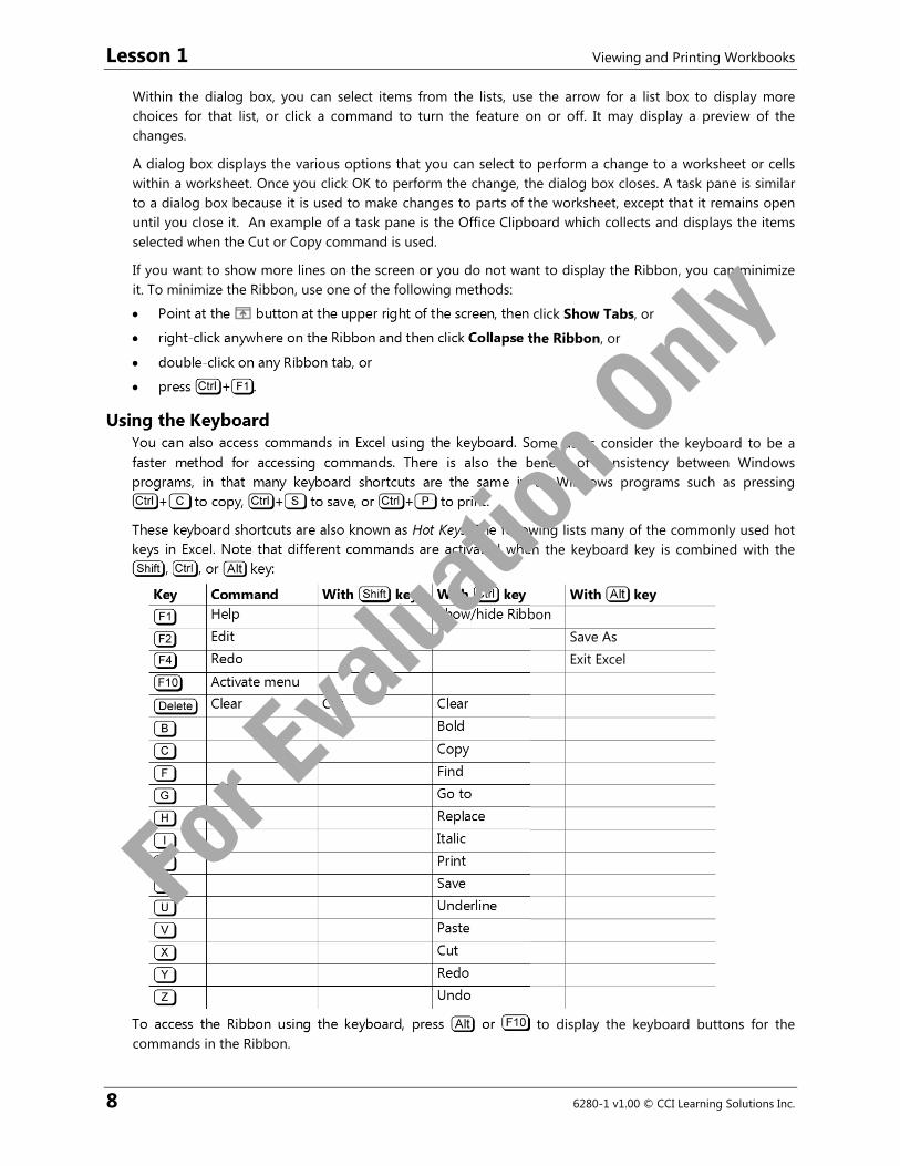
These keyboard shortcuts are also known as Hot Keys. The following lists many of the commonly used hot keys in Excel. Note that different commands are activated when the keyboard key is combined with the

, , or key:

Key Command With key With key With key

Help Show/hide Ribbon

Edit Save As

Redo Exit Excel

Activate menu

Clear Cut Clear

Bold

Copy

Find

Go to

Replace

Italic

Print

Save

Underline

Paste

Cut

Redo

Undo

To access the Ribbon using the keyboard, press or to display the keyboard buttons for the commands in the Ribbon.

For E

valua

tion O

nly



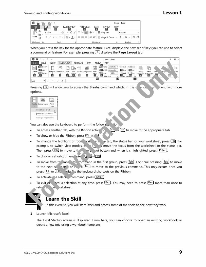
When you press the key for the appropriate feature, Excel displays the next set of keys you can use to select a command or feature. For example, pressing displays the Page Layout tab.

Pressing will allow you to access the Breaks command which, in this case, displays a menu with more options.

You can also use the keyboard to perform the following actions:

To access another tab, with the Ribbon active, press or to move to the appropriate tab.

To show or hide the Ribbon, press + .

To change the highlight or focus from the active tab, the status bar, or your worksheet, press . For example, to switch view modes, press to move the focus from the worksheet to the status bar. Then press to move to the Page Layout button and, when it is highlighted, press .

To display a shortcut menu, press + .

To move from the tab to the command in the first group, press . Continue pressing to move to the next command, or + to move to the previous command. This only occurs once you press or to display the keyboard shortcuts on the Ribbon.

To activate the selected command, press .

To exit or cancel a selection at any time, press . You may need to press more than once to return to your worksheet.

Learn the Skill In this exercise, you will start Excel and access some of the tools to see how they work.

1 Launch Microsoft Excel.

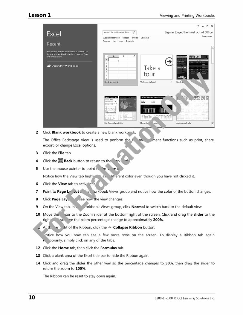
The Excel Startup screen is displayed. From here, you can choose to open an existing workbook or create a new one using a workbook template.

For E

valua

tion O

nly



2 Click Blank workbook to create a new blank workbook.

The Office Backstage View is used to perform the file management functions such as print, share, export, or change Excel options.

3 Click the File tab.

4 Click the Back button to return to the workbook.

5 Use the mouse pointer to point to the View tab.

Notice how the View tab highlights as a different color even though you have not clicked it.

6 Click the View tab to activate it.

7 Point to Page Layout in the Workbook Views group and notice how the color of the button changes.

8 Click Page Layout to see how the view changes.

9 On the View tab, in the Workbook Views group, click Normal to switch back to the default view.

10 Move the cursor to the Zoom slider at the bottom right of the screen. Click and drag the slider to the right until you see the zoom percentage change to approximately 200%.

11 At the far right of the Ribbon, click the Collapse Ribbon button.

Notice how you now can see a few more rows on the screen. To display a Ribbon tab again temporarily, simply click on any of the tabs.

12 Click the Home tab, then click the Formulas tab.

13 Click a blank area of the Excel title bar to hide the Ribbon again.

14 Click and drag the slider the other way so the percentage changes to 50%, then drag the slider to return the zoom to 100%.

The Ribbon can be reset to stay open again.

For E

valua

tion O

nly



15 Click the Ribbon Display Options button, then click Show Tabs and Commands to re-display the entire Ribbon.

16 Now move the cursor to the top of the screen and click some of the tabs to see how the commands are categorized and grouped on the tabs.

17 Press to display the keyboard shortcuts on the tab.

18 Press to display the Page Layout tab.

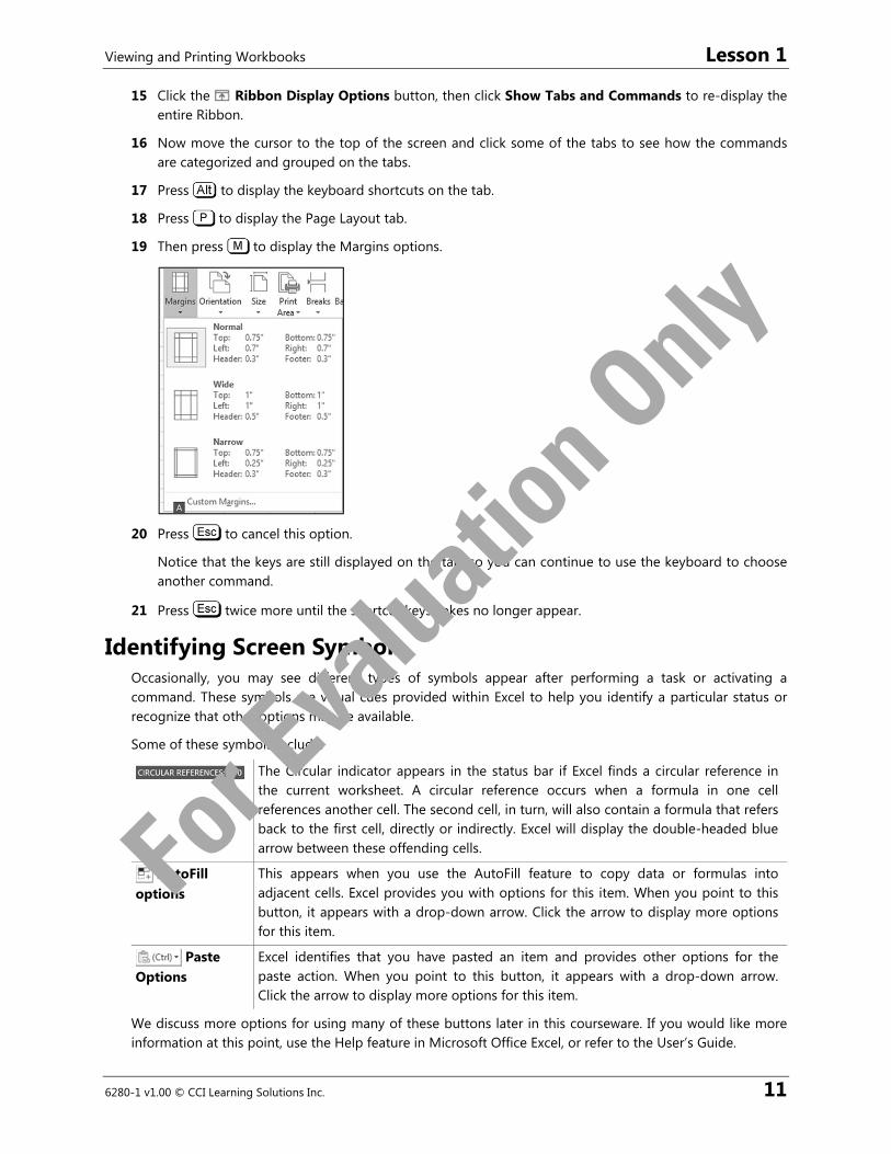
19 Then press to display the Margins options.

20 Press to cancel this option.

Notice that the keys are still displayed on the tab, so you can continue to use the keyboard to choose another command.

21 Press twice more until the shortcut keystrokes no longer appear.

Identifying Screen Symbols Occasionally, you may see different types of symbols appear after performing a task or activating a command. These symbols are visual cues provided within Excel to help you identify a particular status or recognize that other options may be available.

Some of these symbols include:

The Circular indicator appears in the status bar if Excel finds a circular reference in the current worksheet. A circular reference occurs when a formula in one cell references another cell. The second cell, in turn, will also contain a formula that refers back to the first cell, directly or indirectly. Excel will display the double-headed blue arrow between these offending cells.

AutoFill options

This appears when you use the AutoFill feature to copy data or formulas into adjacent cells. Excel provides you with options for this item. When you point to this button, it appears with a drop-down arrow. Click the arrow to display more options for this item.

Paste Options

Excel identifies that you have pasted an item and provides other options for the paste action. When you point to this button, it appears with a drop-down arrow. Click the arrow to display more options for this item.

We discuss more options for using many of these buttons later in this courseware. If you would like more information at this point, use the Help feature in Microsoft Office Excel, or refer to the User’s Guide.

For E

valua

tion O

nly



Entering Data in a Worksheet If you design and build it in a logical manner, an Excel worksheet is a very powerful tool. The basic building block of every worksheet is entering data into the cells.

Types of Data You can make three main types of entries when you insert data into worksheet cells:

Numeric Numeric data form the core of all spreadsheets. This type of data consists of number, date, or time values that you enter directly into a worksheet cell. By default, numeric values align to the right.

Text Text data consist of alphabetic and numeric characters and most printable symbols. Text data are usually labels or titles used to describe and explain the data in adjoining cells. Text is seldom included in calculations, but Excel does include several functions that apply to text data. If you enter a text value that is wider than the cell, it will flow into the adjacent cells as long as those cells are empty. By default, text data align to the left.

Formulas Formulas, which you enter in individual cells, are composed of values, cell references, arithmetic operators, and special functions for calculating and displaying result. These results may then become part of other formulas located in other cells. The ability to use formulas is what differentiates spreadsheets from word processing software like Microsoft Word.

Entering Text To enter data, move your pointer to the desired cell, click in it, and type the entry. If you make a typing error while still entering information in a cell, press the key to erase your mistake. When you have finished entering data in a cell, press the key to move the cell pointer automatically to the next cell down. Alternatively, use your mouse to click another cell (or press any arrow key), which performs the same result of storing the data in that cell and moving the cell pointer to the new location.

The best way to begin any worksheet is to enter column and row titles that identify the purpose of the numeric data. When you enter titles for the worksheet, you are creating an outline of the relationships you will later represent mathematically.

When typing information, notice that Excel displays the text in two places:

You can enter or edit data directly in the active cell where the pointer appears, or you can enter or edit it in the formula bar. The latter method is especially useful for very long data entries. In either case, the data is displayed in both places.

Text entries can be up to 32,767 characters, although a maximum of 255 characters are displayed. If a text entry is longer than the width of the cell, it will extend past the column border after you have pressed , as long as there is nothing entered in the adjoining cells. Entries in adjoining cells truncate the display of the text at the border. The entire entry goes into the cell, but only the portion that fits in the available space is visible. By default, Excel aligns text data on the left side of the cell. You can easily change the appearance and alignment of a text entry.

Learn the Skill This exercise demonstrates how to enter text data into a worksheet cell, which will serve as a label or title for other cells containing numeric data.

1 In a new blank workbook, click in cell A2.

2 Type: Price Quote and press .

For E

valua

tion O

nly



Notice the current active cell is now A3. When you press , Excel completes the entry of data in the current cell, then moves the cell pointer to the next cell down.

3 Press twice to move down two rows.

4 In cell A5, type: Airfare and press .

5 In cell A6, type: Hotel and press .

6 In cell A7, type: Car Rental and press .

7 In cell A8, type: Taxes and press .

Note: If you entered the wrong value into a cell, simply select the cell and type the correct entry again to replace the incorrect value.

Now try a feature called AutoComplete, in which Excel determines whether you are repeating the same text as in a previous cell and completes it for you. If it is the text you want, you simply press to accept it.

8 In cell A9, type: A.

Notice that Excel automatically offers you a text label, based on your previous entry. You can now press

the key to accept it or continue typing the value that you want.

9 Ignore the suggested label and continue typing the rest of the text: irport Fees.

Notice that the text extends further than the default column width for this text entry. If you enter data in the next column, the part of this new label that overflows into the next column will appear to be cut off.

10 In cell A12, type: Airline:

Notice this time that the AutoComplete feature did not turn on. This is because of the blank cells (A10 and A11) that are preventing Excel from “looking up” a previous similar value in this column.

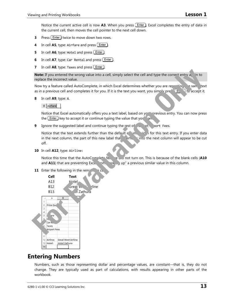
11 Enter the following in the remaining cells:

Cell Text A13 Hotel: B12 Great West Airline B13 Hotel Zathura

Entering Numbers Numbers, such as those representing dollar and percentage values, are constant—that is, they do not change. They are typically used as part of calculations, with results appearing in other parts of the workbook.

For E

valua

tion O

nly



By default, Excel aligns numeric values to the right side of a cell. They are displayed with no commas unless you enter them at the same time. Extraneous zeroes are not displayed, even if entered at the same time. You can format the values to your preference at a later time.

If you enter a value that contains a mixture of alphabetic and numeric digits (for example, T-1000), Excel treats the entire entry as text and aligns it to the left of the cell.

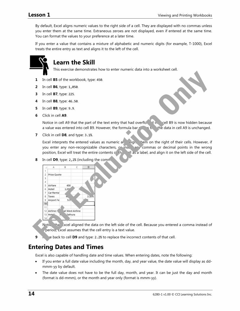
Learn the Skill This exercise demonstrates how to enter numeric data into a worksheet cell.

1 In cell B5 of the workbook, type: 450.

2 In cell B6, type: 1,050.

3 In cell B7, type: 225.

4 In cell B8, type: 46.50.

5 In cell B9, type: 9.9.

6 Click in cell A9.

Notice in cell A9 that the part of the text entry that had overflowed into cell B9 is now hidden because a value was entered into cell B9. However, the formula bar shows that the data in cell A9 is unchanged.

7 Click in cell D8, and type: 3.1%.

Excel interprets the entered values as numeric and aligns them on the right of their cells. However, if you enter any non-recognizable characters, or insert any commas or decimal points in the wrong position, Excel will treat the entire contents of that cell as a label, and align it on the left side of the cell.

8 In cell D9, type: 2,2% (including the comma).

Notice that Excel aligned the data on the left side of the cell. Because you entered a comma instead of

a period, Excel assumes that the cell entry is a text value.

9 Move back to cell D9 and type: 2.2% to replace the incorrect contents of that cell.

Entering Dates and Times Excel is also capable of handling date and time values. When entering dates, note the following:

If you enter a full date value including the month, day, and year value, the date value will display as dd-mmm-yy by default.

The date value does not have to be the full day, month, and year. It can be just the day and month (format is dd-mmm), or the month and year only (format is mmm-yy).

For E

valua

tion O

nly



If you enter only the name of a month, Excel will treat it as a text value. If you enter only a day or year value, Excel will treat it as a numeric value. In these cases, Excel will not recognize that you intended to enter a part of a date value.

When entering the date, Excel attempts to interpret what you have entered. For example, the following are acceptable date values:

September 15, 2013 (you must include the comma followed by a space) Sep 15, 13 15-Sep-13 09/15/13 (month, day, year sequence — see next bullet) 9-15-13 Sep 2013 Sep 15

If you enter the date using only numeric values (for example, 09/15/13 as shown above), the sequence of the values must match the date sequence specified in the Windows Control Panel, Regional and Language Options. For the United States, the normal date sequence is month/day/year. For Canada and the United Kingdom, the sequence is day/month/year. If Excel is not able to interpret the date value, it will appear as a text label (left aligned in the cell).

When entering time values, note the following:

The time must consist of hours and minutes, as a minimum, in the format of hh:mm. You can also add seconds and the AM/PM indicator. The alternative to the latter is to use the 24-hour clock format.

The following are acceptable time values:

1:15 PM (be sure to add a space before the AM/PM indicator) 13:15 13:15:01 1:15:01 PM 1:15

Learn the Skill This exercise demonstrates the use of dates.

1 In cell A3, type: As of: and press .

2 In cell B3 type: 30 Jun and press .

Notice that Excel puts the date in the default format and aligns it to the right.

3 In cell D3 type: Expires: and press .

4 In cell E3 type: Jul 15, 2013 and press . For E

valua

tion O

nly



5 Select cell E3.

The date value for this cell also appears in the formula bar. The date value sequence corresponds to the setting in the Windows Control Panel.

6 Select cell B3.

Because you have not included a year in this date value, Excel assumes it is the current year and adds it for you. If you want a different year, you have to enter it as part of the date.

Moving Around the Worksheet You can move around the cells of a worksheet very quickly by either using the keyboard or scrolling with the mouse. Use one of the following methods to move around in the worksheet:

Scroll Bars Click the arrow buttons at either end of the scroll bars to move one row or column at a time. Click on the scroll box (the size will vary depending on the zoom percentage) and drag to display another location in the worksheet.

, , , Press one of these directional keys to move one cell at a time.

Press this key to move to column A in the current row.

+ Press this key combination to move to cell A1, regardless of where you are in the worksheet.

+ Press this key combination to move to the last cell in the data table.

+ / Display the Go To dialog box so you can move quickly to a cell reference, range name, or bookmark, or use the Special button to find specific types of information (for example, Comments, Blanks)

Working with Workbooks As you begin using workbooks, you need to consider how to organize your files for quick and easy access. This includes considerations such as how you name the file, where you save it, whether it needs to be saved as a specific file type, and whether you want to add or change the file properties to make it easier to find at a later date. The Save commands are located in the Office Backstage View via the File tab.

Saving Workbooks To be able to recall your work later, you must save your workbook before exiting Excel or turning off your computer. The saved file also provides an excellent fall-back option if you try something in your worksheet that does not work as you expected, and you are unable or unwilling to undertake all the necessary steps to correct the problem.

For E

valua

tion O

nly



When naming a workbook, keep the following in mind:

Workbook names must follow the same basic rules as naming files in Windows: a maximum of 255 characters (including the drive and folder path), and none of these characters: / \ : * ? “ < >|

File names should be descriptive so that you can identify the contents quickly.

Excel automatically assigns a .xlsx extension or file type at the end of the file name, so you need not do this. You only have to type in the name for the workbook.

Files can be saved with two different types of save commands:

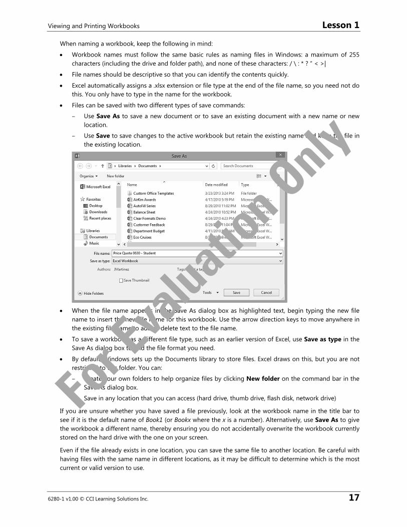
– Use Save As to save a new document or to save an existing document with a new name or new location.

– Use Save to save changes to the active workbook but retain the existing name and keep the file in the existing location.

When the file name appears in the Save As dialog box as highlighted text, begin typing the new file

name to insert the new file name for this workbook. Use the arrow direction keys to move anywhere in the existing file name to add or delete text to the file name.

To save a workbook as a different file type, such as an earlier version of Excel, use Save as type in the Save As dialog box to find the file format you need.

By default, Windows sets up the Documents library to store files. Excel draws on this, but you are not restricted to this folder. You can:

– Create your own folders to help organize files by clicking New folder on the command bar in the Save As dialog box.

– Save in any location that you can access (hard drive, thumb drive, flash disk, network drive)

If you are unsure whether you have saved a file previously, look at the workbook name in the title bar to see if it is the default name of Book1 (or Bookx where the x is a number). Alternatively, use Save As to give the workbook a different name, thereby ensuring you do not accidentally overwrite the workbook currently stored on the hard drive with the one on your screen.

Even if the file already exists in one location, you can save the same file to another location. Be careful with having files with the same name in different locations, as it may be difficult to determine which is the most current or valid version to use.

For E

valua

tion O

nly



To view the file type (the extension part of the file name), you need to turn on this option using File Explorer. Click View, and on the Show/hide group, click File name extensions to activate it. If you are using Windows 7, click Organize, Folder and search options, select the View tab and under the Advanced settings, disable the checkbox for Hide extensions for known file types. Showing the file types can be helpful when determining which file you want to use. For example, two files may have the same name, but the file extensions show that one is in .xlsx format (Excel 2007 and later) while the other is in .xls format (Excel 2003 and earlier).

To save changes made to the current workbook using the same file name, use one of the following methods:

Click File and then Save, or

on the Quick Access Toolbar, click Save, or

press + .

You can use Views in the Save As dialog box to help display the folders and files in the way you prefer (for example, list or thumbnails).

Learn the Skill In this exercise, you will save the new workbook you have just created.

1 In the Quick Access Toolbar, click Save.

The Office Backstage View is displayed, and the Save As command is selected. Even though you clicked Save, Excel will automatically skip to Save As for any new workbook that was never previously saved. The Save command will save the current workbook to disk using the same workbook name and storage location. The Save As command is needed to ask you to assign the workbook name and storage location.

2 Click My Documents. Alternatively, click the Browse button if the desired folder is not displayed under

the Recent Folders or Current Folder headings.

The Save As dialog box is now displayed with the My Documents folder contents displayed.

3 In the left pane of the Save As dialog box, navigate to where the student data files are located for this courseware. Check with your instructor if you are unsure of the location.

Notice that Excel has entered the current title of the workbook as a suggestion for the file name. You can use this name or replace it with a name of your choosing.

For E

valua

tion O

nly



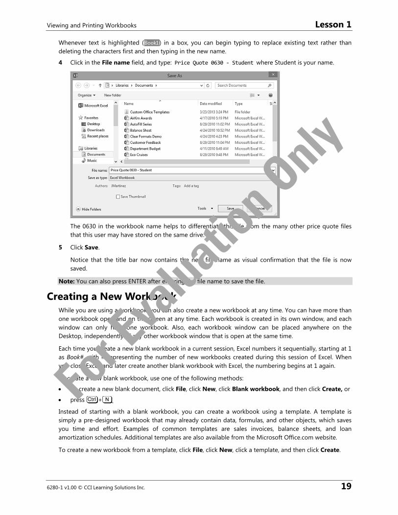
Whenever text is highlighted ( ) in a box, you can begin typing to replace existing text rather than deleting the characters first and then typing in the new name.

4 Click in the File name field, and type: Price Quote 0630 ‐ Student where Student is your name.

The 0630 in the workbook name helps to differentiate this file from the many other price quote files

that this user may have stored on the same drive.

5 Click Save.

Notice that the title bar now contains the new file name as visual confirmation that the file is now saved.

Note: You can also press ENTER after entering the file name to save the file.

Creating a New Workbook While you are using a workbook, you can also create a new workbook at any time. You can have more than one workbook open and on the screen at any time. Each workbook is created in its own window, and each window can only have one workbook. Also, each workbook window can be placed anywhere on the Desktop, independently of any other workbook window that is open at the same time.

Each time you create a new blank workbook in a current session, Excel numbers it sequentially, starting at 1 as Book#, with # representing the number of new workbooks created during this session of Excel. When you close Excel, and later create another blank workbook with Excel, the numbering begins at 1 again.

To create a new blank workbook, use one of the following methods:

To create a new blank document, click File, click New, click Blank workbook, and then click Create, or

press + .

Instead of starting with a blank workbook, you can create a workbook using a template. A template is simply a pre-designed workbook that may already contain data, formulas, and other objects, which saves you time and effort. Examples of common templates are sales invoices, balance sheets, and loan amortization schedules. Additional templates are also available from the Microsoft Office.com website.

To create a new workbook from a template, click File, click New, click a template, and then click Create.

For E

valua

tion O

nly



Learn the Skill In this exercise, you will create a new workbook using different methods.

1 Press + .

You should now have a new blank workbook titled as Book2 on the screen, appearing in front of any other workbooks currently open.

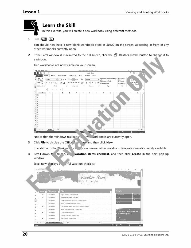
2 If the Excel window is maximized to the full screen, click the Restore Down button to change it to a window.

Two workbooks are now visible on your screen.

Notice that the Windows taskbar shows two workbooks are currently open.

3 Click File to display the Office Backstage and then click New.

In addition to the Blank workbook option, several other workbook templates are also readily available.

4 Scroll down the screen, click Vacation items checklist, and then click Create in the next pop-up window.

Excel now displays a colorful vacation checklist.

For E

valua

tion O

nly



This is an example of how templates can save you time and effort when creating a workbook. Many of the elements you see in this document will be covered in more depth later in this courseware.

You can also select from your own templates, from Microsoft’s website, or other Internet websites. To use templates from Microsoft’s website, use the search feature.

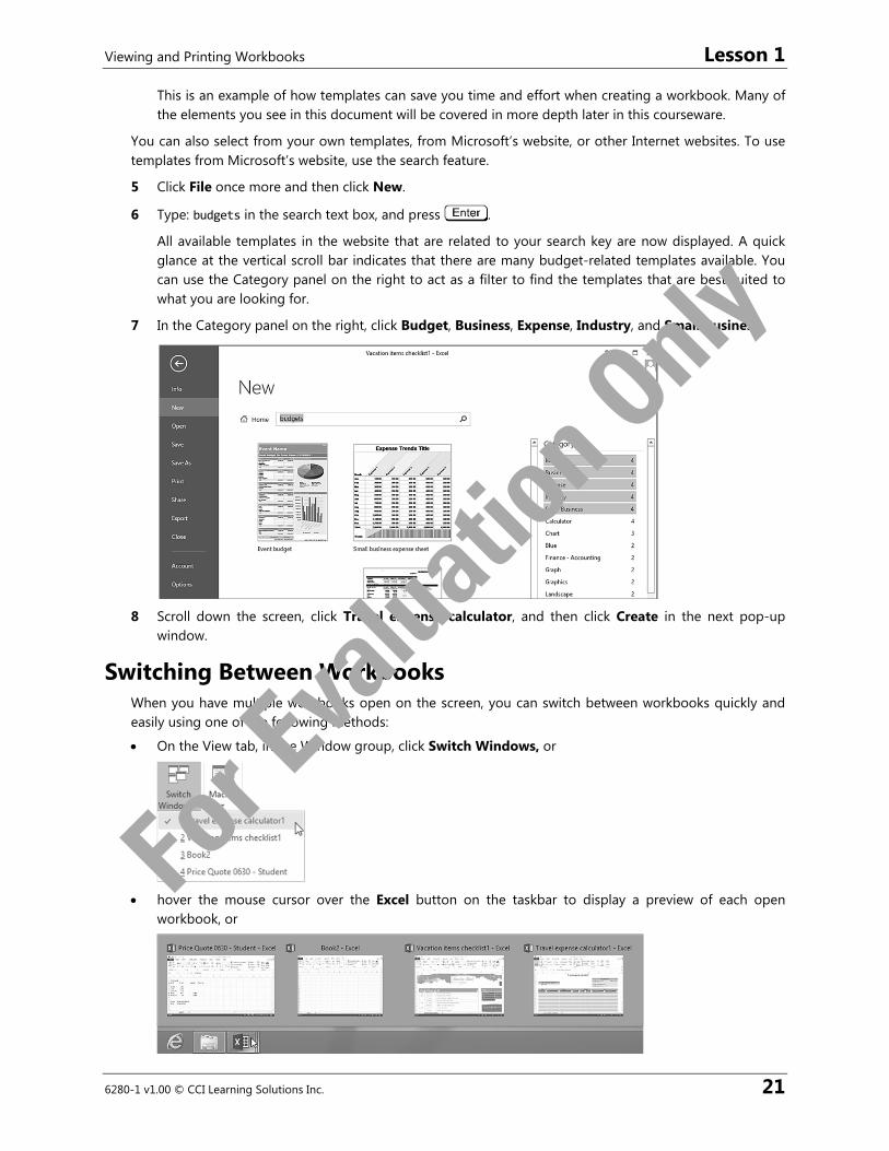
5 Click File once more and then click New.

6 Type: budgets in the search text box, and press .

All available templates in the website that are related to your search key are now displayed. A quick glance at the vertical scroll bar indicates that there are many budget-related templates available. You can use the Category panel on the right to act as a filter to find the templates that are best suited to what you are looking for.

7 In the Category panel on the right, click Budget, Business, Expense, Industry, and Small Business.

8 Scroll down the screen, click Travel expense calculator, and then click Create in the next pop-up

window.

Switching Between Workbooks When you have multiple workbooks open on the screen, you can switch between workbooks quickly and easily using one of the following methods:

On the View tab, in the Window group, click Switch Windows, or

hover the mouse cursor over the Excel button on the taskbar to display a preview of each open workbook, or

For E

valua

tion O

nly



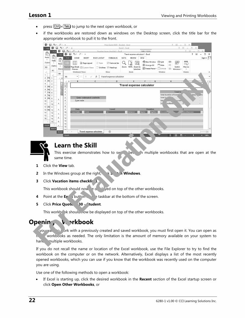
press + to jump to the next open workbook, or

if the workbooks are restored down as windows on the Desktop screen, click the title bar for the appropriate workbook to pull it to the front.

Learn the Skill This exercise demonstrates how to switch between multiple workbooks that are open at the same time.

1 Click the View tab.

2 In the Windows group at the right, click Switch Windows.

3 Click Vacation items checklist1.

This workbook should now be displayed on top of the other workbooks.

4 Point at the Excel button on the taskbar at the bottom of the screen.

5 Click Price Quote 0630 - Student.

This workbook should now be displayed on top of the other workbooks.

Opening a Workbook If you want to work with a previously created and saved workbook, you must first open it. You can open as many workbooks as needed. The only limitation is the amount of memory available on your system to handle multiple workbooks.

If you do not recall the name or location of the Excel workbook, use the File Explorer to try to find the workbook on the computer or on the network. Alternatively, Excel displays a list of the most recently opened workbooks, which you can use if you know that the workbook was recently used on the computer you are using.

Use one of the following methods to open a workbook:

If Excel is starting up, click the desired workbook in the Recent section of the Excel startup screen or click Open Other Workbooks, or

For E

valua

tion O

nly



right-click on the Excel Quick Launch icon in the taskbar and select the recently used workbook from the jump list, or

with a workbook currently open, click File, click Open, and then click the file from the list of Recent Workbooks, or

As you open workbooks, Excel displays the files in the same order as you opened them, with the most recent at the top of the list. As you reach the maximum number of files that show in this list, the oldest drops from the list. You can click the pin icon at the right of the file name to make this file always available in the list until it is unpinned. By default, you can see a list of up to 50 recent workbooks at a time. This number can be customized.

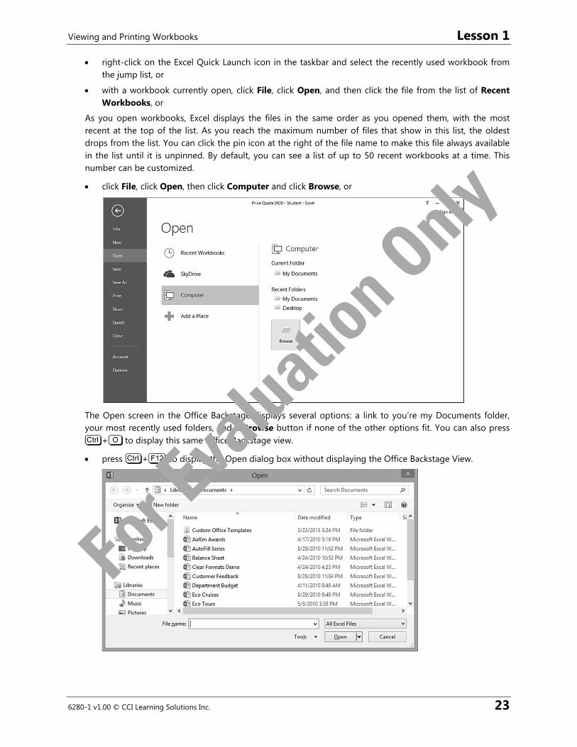
click File, click Open, then click Computer and click Browse, or

The Open screen in the Office Backstage displays several options: a link to you’re my Documents folder, your most recently used folders, and a Browse button if none of the other options fit. You can also press

+ to display this same Office Backstage view.

press + to display the Open dialog box without displaying the Office Backstage View.

For E

valua

tion O

nly



Once the Open dialog box displays, you can navigate using the mouse or keyboard to display the files or folders and then use one of the following methods to open a document:

Double-click the file name, or

click on the file name to select it, and then click Open or press , or

if the file is stored in a different location, navigate to the location and then use one of the above methods to open a file.

Closing a Workbook Once you have finished creating or updating a workbook, close it to clear the screen and free up computer memory. This ensures that any unsaved data for that workbook is saved onto the hard drive, and protects the workbook from unintended changes. Closing your workbook is much like closing a book and putting it back on the shelf before opening another book.

If you try to close a workbook containing unsaved changes, Excel displays a message to advise you of the unsaved changes. You can then choose to close the workbook without saving the changes, or save the changes and close the workbook.

You can use one of the following methods to close a workbook:

click File and then Close, or

press + or + , or

click the Close button.

Note: Because each workbook is running in its own Excel application window, closing one workbook will not affect any other open workbooks.

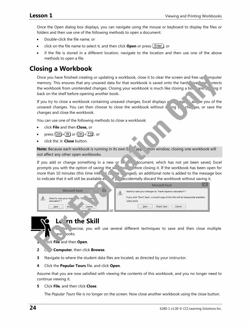
If you add or change something in a new or existing document, which has not yet been saved, Excel prompts you with the option of saving the workbook before closing it. If the workbook has been open for more than 10 minutes (this time interval can be changed), an additional note is added to the message box to indicate that it will still be available even if you accidentally discard the workbook without saving it.

or

Learn the Skill In this exercise, you will use several different techniques to save and then close multiple workbooks.

1 Click File and then Open.

2 Click Computer, then click Browse.

3 Navigate to where the student data files are located, as directed by your instructor.

4 Click the Popular Tours file, and click Open.

Assume that you are now satisfied with viewing the contents of this workbook, and you no longer need to continue viewing it.

5 Click File, and then click Close.

The Popular Tours file is no longer on the screen. Now close another workbook using the close button.

For E

valua

tion O

nly



6 On the View tab, in the Windows group, click Switch Windows.

7 Click Vacation items checklist1.

8 Click the Close button in the upper right corner of this workbook.

9 If a pop-up message box is displayed with this question: “Do you want to save the changes you made to Vacation items checklist1?”, click Don’t Save.

Close another workbook, but use the close button in the taskbar preview this time.

10 Point to the Excel button in the taskbar, then point to the EventBudget1 workbook, and click the Close button for that workbook. Click Don’t Save in the pop-up message box if it appears.

11 Point to the Excel button in the taskbar, then click on the Book2 workbook to make it active, and press + . Click Don’t Save in the pop-up message box if it appears.

12 Click the Close button in the upper right corner of the remaining Price Quote 0630 – Student workbook.

All workbooks should now be closed. And because there no other workbooks currently open, Excel will also be closed.

Working with the Compatibility Mode Excel provides two different formats for saving your workbooks if you need to share it with other people who may be using an older version of Excel. Versions older than Excel 2007 are not able to open workbooks that use the .xlsx format, unless an additional add-in is installed. To save a workbook in an older Excel format to enable these older versions of Excel to use it, click File, click Save As and then click the arrow for Save as type to choose either Excel 97-2003 Workbook or the much older Microsoft Excel 5.0/95 Workbook format.

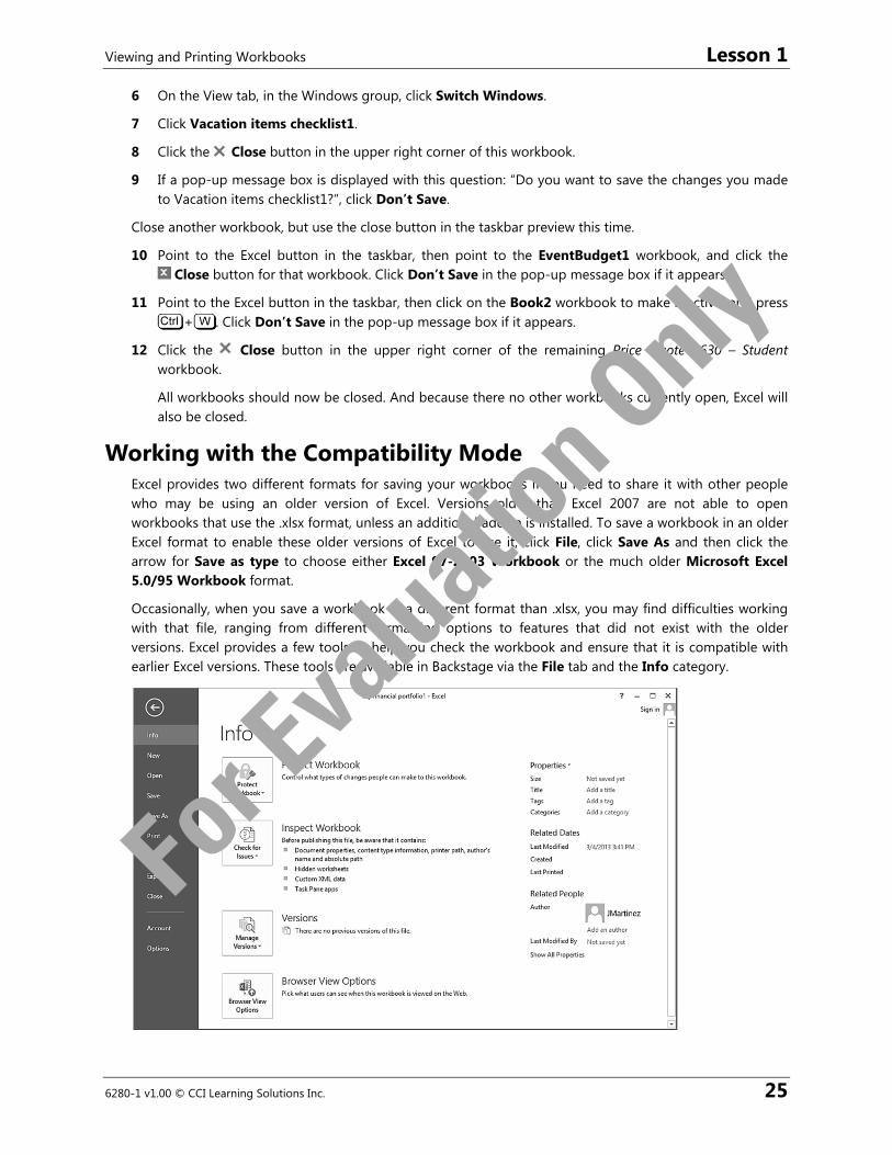
Occasionally, when you save a workbook in a different format than .xlsx, you may find difficulties working with that file, ranging from different formatting options to features that did not exist with the older versions. Excel provides a few tools to help you check the workbook and ensure that it is compatible with earlier Excel versions. These tools are available in Backstage via the File tab and the Info category.

For E

valua

tion O

nly



To check if there may be problems with converting your workbook to a different file format than .xlsx, click File, click Info, click Check for Issues, and then Check Compatibility.

Any potential problems between the versions appear in the list. You then need to decide whether to continue saving the file in this file format or return to the document to make appropriate changes.

Learn the Skill In this exercise, you will check a workbook for compatibility before saving it in the .xls format.

1 Start Excel.

2 In the Excel startup screen, click My financial portfolio to create a new workbook using this template, then click Create in the pop-up window that appears next.

3 Click File.

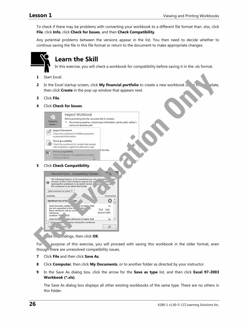
4 Click Check for Issues.

5 Click Check Compatibility.

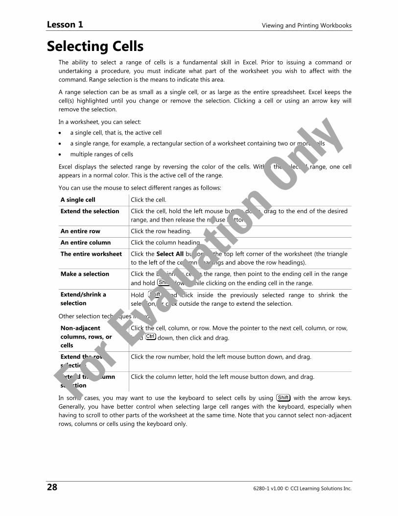
6 Read the findings, then click OK.

For the purpose of this exercise, you will proceed with saving this workbook in the older format, even though there are unresolved compatibility issues.

7 Click File and then click Save As.

8 Click Computer, then click My Documents, or to another folder as directed by your instructor.

9 In the Save As dialog box, click the arrow for the Save as type list, and then click Excel 97-2003 Workbook (*.xls).

The Save As dialog box displays all other existing workbooks of the same type. There are no others in this folder.

For E

valua

tion O

nly



10 Change the File name to My financial portfolio ‐ Student and click Save.

The Compatibility Checker dialog box is displayed again as a warning.

11 Click Continue.

This message box describes some of the problems you may have when using the older version of Excel.

The Compatibility Checker dialog box gave you the details of the differences. Because this is a standard warning for any workbook containing formulas, these problems may not apply to this workbook.

12 Click Yes.

13 Close the workbook.

14 Start Excel and select the My financial portfolio - Student workbook to open it.

The workbook name in the title bar now shows the label [Compatibility Mode] next to it. This indicates that this workbook uses the file format for an earlier version of Excel.

15 Close the workbook again and don’t save any changes.

For E

valua

tion O

nly



Selecting Cells The ability to select a range of cells is a fundamental skill in Excel. Prior to issuing a command or undertaking a procedure, you must indicate what part of the worksheet you wish to affect with the command. Range selection is the means to indicate this area.

A range selection can be as small as a single cell, or as large as the entire spreadsheet. Excel keeps the cell(s) highlighted until you change or remove the selection. Clicking a cell or using an arrow key will remove the selection.

In a worksheet, you can select:

a single cell, that is, the active cell

a single range, for example, a rectangular section of a worksheet containing two or more cells

multiple ranges of cells

Excel displays the selected range by reversing the color of the cells. Within the selected range, one cell appears in a normal color. This is the active cell of the range.

You can use the mouse to select different ranges as follows:

A single cell Click the cell.

Extend the selection Click the cell, hold the left mouse button down, drag to the end of the desired range, and then release the mouse button.

An entire row Click the row heading.

An entire column Click the column heading.

The entire worksheet Click the Select All button in the top left corner of the worksheet (the triangle to the left of the column headings and above the row headings).

Make a selection Click the beginning cell in the range, then point to the ending cell in the range and hold down while clicking on the ending cell in the range.

Extend/shrink a selection

Hold and click inside the previously selected range to shrink the selection, or click outside the range to extend the selection.

Other selection techniques include:

Non-adjacent columns, rows, or cells

Click the cell, column, or row. Move the pointer to the next cell, column, or row, hold down, then click and drag.

Extend the row selection

Click the row number, hold the left mouse button down, and drag.

Extend the column selection

Click the column letter, hold the left mouse button down, and drag.

In some cases, you may want to use the keyboard to select cells by using with the arrow keys. Generally, you have better control when selecting large cell ranges with the keyboard, especially when having to scroll to other parts of the worksheet at the same time. Note that you cannot select non-adjacent rows, columns or cells using the keyboard only.

For E

valua

tion O

nly



Learn the Skill This exercise demonstrates how to select ranges of cells using the mouse in a blank worksheet so you can quickly identify the ranges.

1 Start Excel with a new blank workbook.

2 Select a single cell by clicking cell A9.

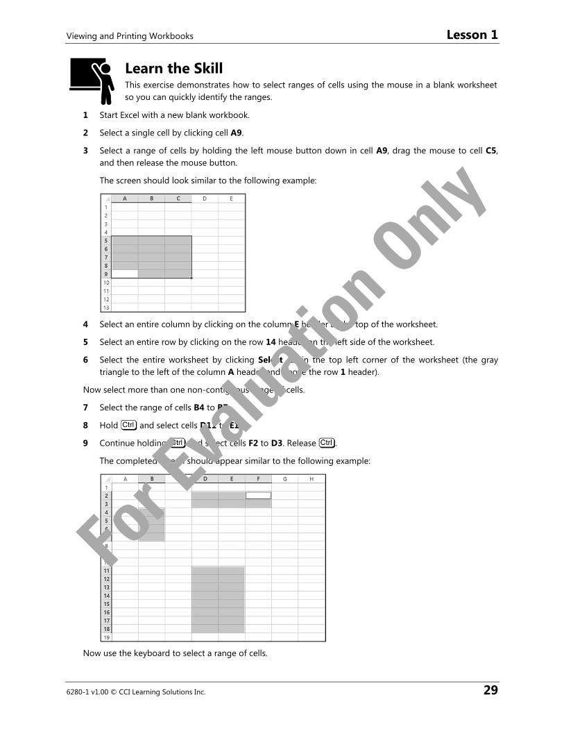
3 Select a range of cells by holding the left mouse button down in cell A9, drag the mouse to cell C5, and then release the mouse button.

The screen should look similar to the following example:

4 Select an entire column by clicking on the column E header at the top of the worksheet.

5 Select an entire row by clicking on the row 14 header on the left side of the worksheet.

6 Select the entire worksheet by clicking Select All in the top left corner of the worksheet (the gray triangle to the left of the column A header and above the row 1 header).

Now select more than one non-contiguous range of cells.

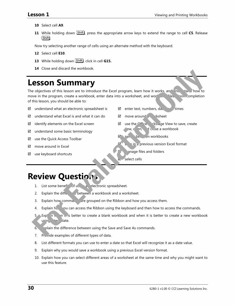
7 Select the range of cells B4 to B7.

8 Hold and select cells D11 to E18.

9 Continue holding and select cells F2 to D3. Release .

The completed screen should appear similar to the following example:

Now use the keyboard to select a range of cells.

For E

valua

tion O

nly



10 Select cell A9.

11 While holding down , press the appropriate arrow keys to extend the range to cell C5. Release .

Now try selecting another range of cells using an alternate method with the keyboard.

12 Select cell E10.

13 While holding down , click in cell G15.

14 Close and discard the workbook.

Lesson SummaryThe objectives of this lesson are to introduce the Excel program, learn how it works, and understand how to move in the program, create a workbook, enter data into a worksheet, and work with files. Upon completion of this lesson, you should be able to:

understand what an electronic spreadsheet is

understand what Excel is and what it can do

identify elements on the Excel screen

understand some basic terminology

use the Quick Access Toolbar

move around in Excel

use keyboard shortcuts

enter text, numbers, dates and times

move around a worksheet

use the Office Backstage View to save, create new, open, and close a workbook

switch between workbooks

save in a previous version Excel format

manage files and folders

select cells

Review Questions 1. List some benefits of using an electronic spreadsheet.

2. Explain the difference between a workbook and a worksheet.

3. Explain how commands are grouped on the Ribbon and how you access them.

4. Explain how you can access the Ribbon using the keyboard and then how to access the commands.

5. Explain when it is better to create a blank workbook and when it is better to create a new workbook using a template.

6. Explain the difference between using the Save and Save As commands.

7. Provide examples of different types of data.

8. List different formats you can use to enter a date so that Excel will recognize it as a date value.

9. Explain why you would save a workbook using a previous Excel version format.

10. Explain how you can select different areas of a worksheet at the same time and why you might want to use this feature.

For E

valua

tion O

nly