Chapter 3: Excel Insert Tab in Excel 2016Last update: 6/16/2019

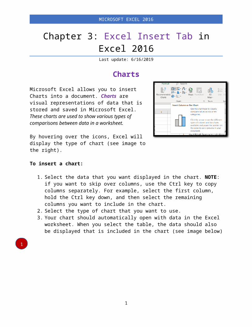
ChartsMicrosoft Excel allows you to insert Charts into a document. Charts are visual representations of data that is stored and saved in Microsoft Excel. These charts are used to show various types of comparisons between data in a worksheet.

By hovering over the icons, Excel will display the type of chart (see image to the right).

To insert a chart:

1. Select the data that you want displayed in the chart. NOTE: if you want to skip over columns, use the Ctrl key to copy columns separately. For example, select the first column, hold the Ctrl key down, and then select the remaining columns you want to include in the chart.

2. Select the type of chart that you want to use. 3. Your chart should automatically open with data in the Excel worksheet. When you select

the table, the data should also be displayed that is included in the chart (see image below)

In the Name box, the Chart Name will appear (see #1 above).

Also note, that on the right side of the chart, you have three different tools (see image to the right). You can use these tools to style your chart.

1

Microsoft excel 2016

1

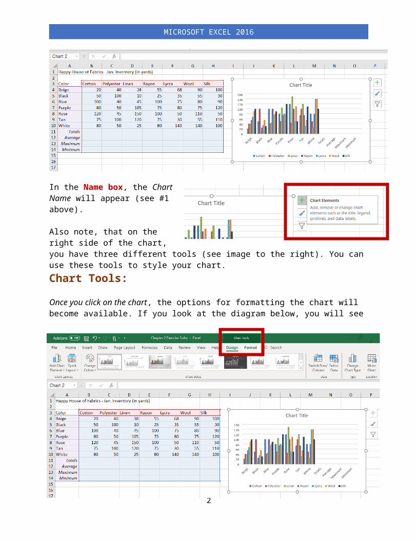
Chart Tools:Once you click on the chart, the options for formatting the chart will become available. If you look at the diagram below, you will see that “Chart Tools” has appeared on the Title bar. You have two different options: Design & Format.

DesignThe Design Toolbar option allows you to change the type of chart, the color of the chart, the chart styles and select and edit data in the chart. There are four ribbons on the Design toolbar:

Chart Layouts, Chart Styles, Data and Type. None of these ribbons have dialog boxes.

Chart Layouts Ribbon:

You have two options when selecting Chart Layouts. They are as follows:

Add Chart Element: by clicking on the drop down arrow, you can add a chart element to the chart (see image to the left). NOTE: you have the same options given to you when you click on the + sign to the right of the chart.

2

Microsoft excel 2016

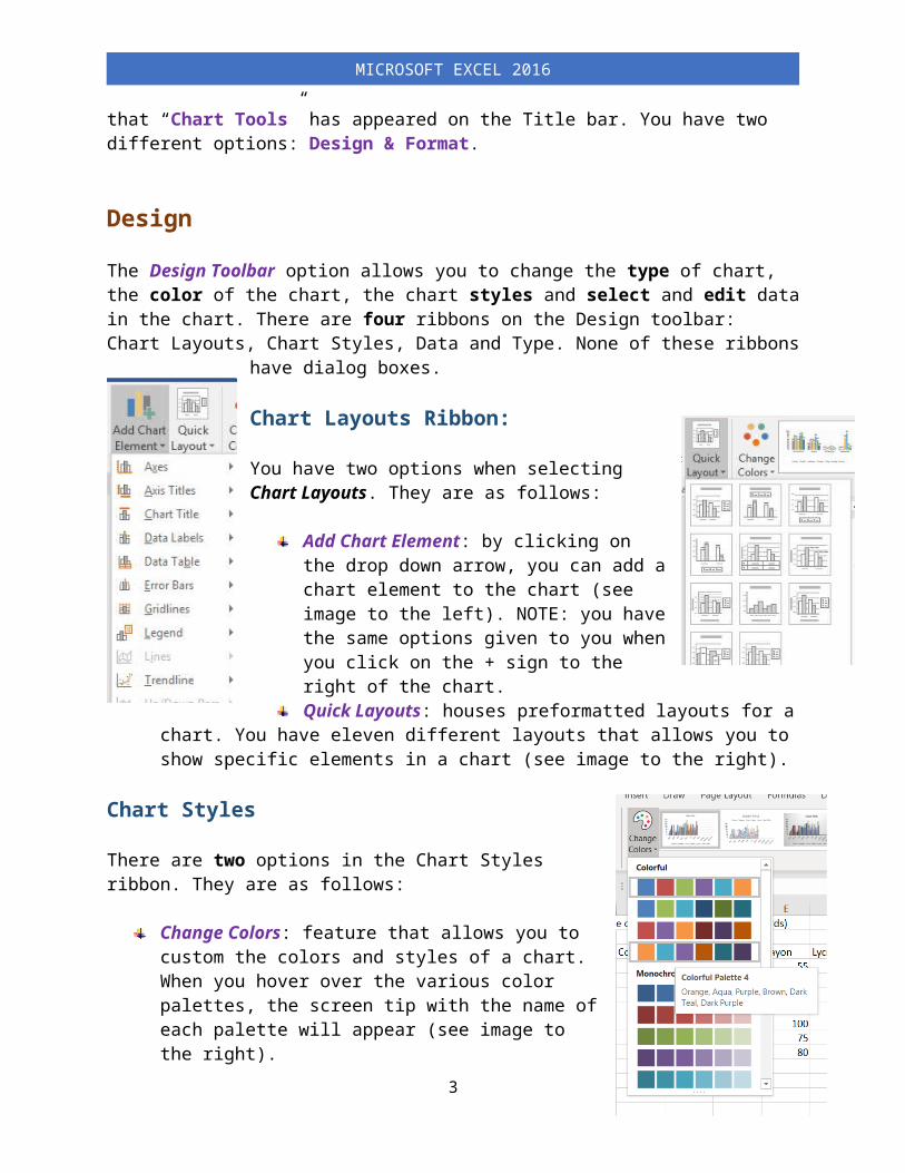
Quick Layouts: houses preformatted layouts for a chart. You have eleven different layouts that allows you to show specific elements in a chart (see image to the right).

Chart Styles

There are two options in the Chart Styles ribbon. They are as follows:

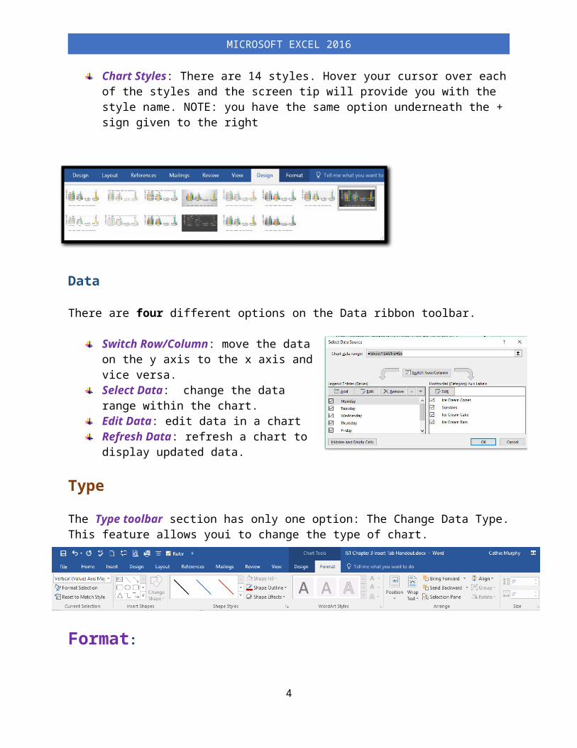
Change Colors: feature that allows you to custom the colors and styles of a chart. When you hover over the various color palettes, the screen tip with the name of each palette will appear (see image to the right).Chart Styles: There are 14 styles. Hover your cursor over each of the styles and the screen tip will provide you with the style name. NOTE: you have the same option underneath the + sign given to the right

Data

There are four different options on the Data ribbon toolbar.

Switch Row/Column: move the data on the y axis to the x axis and vice versa.Select Data: change the data range within the chart.Edit Data: edit data in a chart Refresh Data: refresh a chart to display updated data.

TypeThe Type toolbar section has only one option: The Change Data Type. This feature allows youi to change the type of chart.

3

Microsoft excel 2016

Format:

The Format Toolbar option allows you to format or change how the chart appears. There are six ribbons on the Format toolbar: Current Selection, Insert Shapes, Shape Styles, WordArt Styles, Arrange and Size. Of those six ribbons, three of them have dialog boxes: Shape Styles, WordArt Styles and Size. The dialog boxes will be presented first.

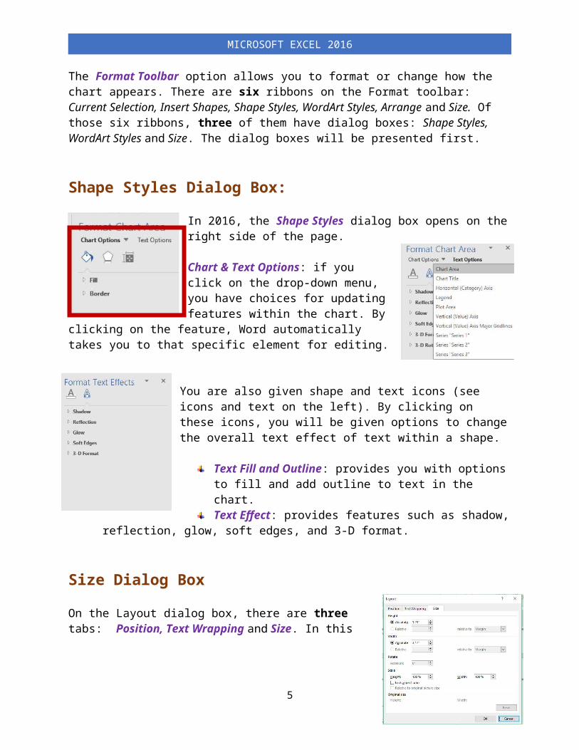
Shape Styles Dialog Box:In 2016, the Shape Styles dialog box opens on the right side of the page.

Chart & Text Options: if you click on the drop-down menu, you have choices for updating features within the chart. By clicking on the feature, Word automatically takes you to that specific element for

editing.

You are also given shape and text icons (see icons and text on the left). By clicking on these icons, you will be given options to change the overall text effect of text within a shape.

Text Fill and Outline: provides you with options to fill and add outline to text in the chart.Text Effect: provides features such as shadow, reflection, glow, soft edges, and 3-D format.

Size Dialog BoxOn the Layout dialog box, there are three tabs: Position, Text Wrapping and Size. In this section, we will only review the Size tab since the other tabs will be discussed elsewhere. 8157212002

On the Size tab, there are four sections.

Height: Width:RotateScale

4

Microsoft excel 2016

Under the Height and Width options, you have two choices: “absolute” or “relative”. Under the Absolute option, you will have to decide how many pixels that you want applied to the chart in regards to height and width. Under the Relative option, you will need to change both the size relative to a position (i.e. margin, column, etc.)

The Lock Aspect Ratio: When you want to change the width, but not the height, turn off the lock aspect ration feature. When the lock aspect ratio feature is turned on, Word will automatically adjust the dimensions so that the image does not become distorted. To stop this automcatic adjustment, turn off the feature.

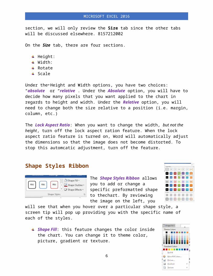
Shape Styles RibbonThe Shape Styles Ribbon allows you to add or change a specific preformatted shape to thechart. By reviewing the image on the left, you will see that when you hover over a particular shape style, a

screen tip will pop up providing you with the specific name of each of the styles.

Shape Fill: this feature changes the color inside the chart. You can change it to theme color, picture, gradient or texture.Shape Outline: This feature changes the border around the shape.Shape Effects: This feature adds effects such as shadow, glow, 3-D effect, bevel and soft edges.

Alternate Text for a ChartThe alternate text allows you to create descriptions for screen readers. To add “Alt Text” information, right click on the Chart and select Table Properties. One of the tabs that will appear on the Table Properites box is “Alt Text.”Function IconOn the Home tab in Excel, you can quickly access the Insert Function action by clicking on the icon. The positive thing about using the Insert Function option, is that you do not need to know exactly how to write a formula.

For example, let’s say that you have a problem as follows: In cell I7 of the New Releases worksheet, use a function to calculate the average of the Review Score column where the System type is YCube 720.

5

Microsoft excel 2016

You will have this exercise in your series of exercises. What would you do?

1. On the New Releases worksheet, click cell I7.2. In the Formula Bar, type =AVERAGEIF, then press the tab key on your keyboard.3. To the left of the Formula Bar, click fx to open the Function Arguments wizard.4. In the Function Arguments wizard, configure the following:

a) Range: B7:B19 b) Criteria: YCube 720c) Average_Range: E7:E19d) Click OK.

Name BoxThe Name Box in Excel is used for more than just searching for a cell. You can also use it to search for defined names. When you use the Name Box to search for define names, it will search for it and then select the cells that are included in the Defined name. Using the name box is quicker when you want to delete cells within the defined name.

Convert to Range FeatureAfter you create an Excel table, you may only want the table style without the table functionality. To stop working with your data in a table without losing any table style formatting that you applied, you can convert the table to a regular range of data on the worksheet. To do this use, the Convert to Range icon underneath the Tools section of Table Tools Design. Find the name of the table in the Name box, and then go to Table Tools Design, select “Convert to Range” and then “yes”.

6

Microsoft excel 2016