Contents

1 Network Parameters of a Two-Port Filter 11.1 S Parameters in the s-domain . . . . . . . . . . . . . . . . . . . . . . . . . . . . 1

1.1.1 Relation between ε and εR . . . . . . . . . . . . . . . . . . . . . . . . . 21.1.2 Derivation of S22 . . . . . . . . . . . . . . . . . . . . . . . . . . . . . . 3

1.2 Network Parameters in the jω-domain . . . . . . . . . . . . . . . . . . . . . . . 31.2.1 S Parameters in the jω-domain . . . . . . . . . . . . . . . . . . . . . . 31.2.2 ABCD Parameters in the jω-domain . . . . . . . . . . . . . . . . . . . 41.2.3 Y Parameters in the jω-domain . . . . . . . . . . . . . . . . . . . . . . 41.2.4 Z Parameters in the jω-domain . . . . . . . . . . . . . . . . . . . . . . 4

2 Lowpass Prototype Filters 52.1 Basic Components of a Lowpass Prototype Filter . . . . . . . . . . . . . . . . . 52.2 Electric and Magnetic Couplings . . . . . . . . . . . . . . . . . . . . . . . . . . 52.3 ε and εR Values for the Prototype Filters . . . . . . . . . . . . . . . . . . . . . . 72.4 Alternating Pole Method for Determination of E (jω) . . . . . . . . . . . . . . . 72.5 The N Coupling Matrix . . . . . . . . . . . . . . . . . . . . . . . . . . . . . . . 10

2.5.1 Analysis of the General N Coupling Matrix . . . . . . . . . . . . . . . . 102.5.1.1 Series Type LPP . . . . . . . . . . . . . . . . . . . . . . . . . 102.5.1.2 Shunt Type LPP . . . . . . . . . . . . . . . . . . . . . . . . . 11

2.5.2 Synthesis of the General N Coupling Matrix . . . . . . . . . . . . . . . 122.5.2.1 Series Type LPP . . . . . . . . . . . . . . . . . . . . . . . . . 122.5.2.2 Shunt Type LPP . . . . . . . . . . . . . . . . . . . . . . . . . 15

2.6 The N + 2 Coupling Matrix . . . . . . . . . . . . . . . . . . . . . . . . . . . . 152.6.1 Analysis of the General N + 2 Coupling Matrix . . . . . . . . . . . . . . 15

2.6.1.1 Series Type LPP . . . . . . . . . . . . . . . . . . . . . . . . . 152.6.1.2 Shunt Type LPP . . . . . . . . . . . . . . . . . . . . . . . . . 17

2.6.2 Synthesis of the General N + 2 Coupling Matrix . . . . . . . . . . . . . 172.6.2.1 Series Type LPP . . . . . . . . . . . . . . . . . . . . . . . . . 172.6.2.2 Shunt Type LPP . . . . . . . . . . . . . . . . . . . . . . . . . 18

2.6.3 Synthesis of the N + 2 Transversal Matrix . . . . . . . . . . . . . . . . 18

Chapter 1

Network Parameters of a Two-Port Filter

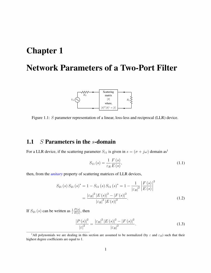
Figure 1.1: S parameter representation of a linear, loss-less and reciprocal (LLR) device.

1.1 S Parameters in the s-domainFor a LLR device, if the scattering parameter S11 is given in s = (σ + jω) domain as1

S11 (s) =1

εR

F (s)

E (s), (1.1)

then, from the unitary property of scattering matrices of LLR devices,

S21 (s)S21 (s)∗ = 1− S11 (s)S11 (s)∗ = 1− 1

|εR|2

∣∣∣∣F (s)

E (s)

∣∣∣∣2=|εR|2 |E (s)|2 − |F (s)|2

|εR|2 |E (s)|2. (1.2)

If S21 (s) can be written as 1εP (s)E(s)

, then

|P (s)|2

|ε|2=|εR|2 |E (s)|2 − |F (s)|2

|εR|2. (1.3)

1All polynomials we are dealing in this section are assumed to be normalized (by ε and εR) such that theirhighest degree coefficients are equal to 1.

1

Also, re-arranging (1.2) and (1.3) gives

|S21 (s)|2 =1

1 +∣∣∣ εεR ∣∣∣2 ∣∣∣F (s)

P (s)

∣∣∣2 , (1.4)

whereF (s)P (s)

is referred to as characteristic function. Before proceeding further, some importantproperties of the polynomials E (s), F (s) and P (s) are given2 here.

1. E (s) is a Hurwitz polynomial of degree N . All its roots lie in the left half-plane of s.

2. The roots of F (s) lie on the imaginary axis where the degree is N . These roots are knownas reflection zeros.

3. Zeros of the polynomial P (s) are known as transmission zeros (TX zeros). All TX zeroslie on the imaginary axis or appear as pairs of zeros located symmetrically with respect tothe imaginary axis.3

As a result, the polynomials E (s), F (s) and P (s) have the forms

E (s) = sN + eN−1sN−1 + eN−2s

N−2 + eN−3sN−3 + · · ·+ e0,

F (s) = sN + jfN−1sN−1 + fN−2s

N−2 + jfN−3sN−3 + · · ·+ f0 and

P (s) = snfz + jpnfz−1snfz−1 + pnfz−2s

nfz−2 + jpnfz−3snfz−3 + · · ·+ p0. (1.5)

In the above equations, all the coefficients ei are complex. Except f0 and p0, all other parametersfi and pi are real. Since the coefficients of F (s) and P (s) alternate between real and imaginarynumbers, f0 and p0 are real if N and nfz are even (and imaginary if their orders are odd).

Also, the following statements can be proved without much difficulty.

at s = 0 :

{S11 = 1

εR

f0e0

S21 = 1εp0e0

(1.6)

at s = ±j∞ :

S11 = 1

εR

S21 = 0, if nfz < N

S21 = 1ε, if nfz = N

(1.7)

1.1.1 Relation between ε and εRAs mentioned before, ε and εR are just some complex numbers for normalizing all the polyno-mials. The relation between these two parameters can be derived from the equation

S11 (s)S11 (s)∗ + S21 (s)S21 (s)∗ = 1

⇒ 1

|εR|2F (s)F (s)∗

E (s)E (s)∗+

1

|ε|2P (s)P (s)∗

E (s)E (s)∗= 1. (1.8)

2For the time being, these properties are stated without any proof.3If nfz , the degree of the polynomial P (s) is zero, then all transmission zeros are located at s = ±j∞ (e.g.,

conventional Butterworth, Chebyshev, etc.).

2

At s = 0, (1.8) becomes

S11 (s)S11 (s)∗ + S21 (s)S21 (s)∗ = 1

⇒ 1

|εR|2

∣∣∣∣f0e0∣∣∣∣2 +

1

|ε|2

∣∣∣∣p0e0∣∣∣∣2 = 1. (1.9)

Similarly, at s = ±j∞, {|εR| = 1, if nfz < N

1|εR|2

+ 1|ε|2 = 1, if nfz = N

. (1.10)

So, from (1.9) and (1.10)

if nfz < N :

{|εR| = 1,

|ε|2 = |p0|2

|e0|2−|f0|2.

(1.11)

if nfz = N :

|ε|2 = |f0|2−|p0|2

|f0|2−|e0|2,

|εR|2 = |f0|2−|p0|2

|e0|2−|p0|2.

(1.12)

��

�

It is important to understand that only |εR| and |ε| are related to each other, but not ∠ε and ∠εR.The phases can be changed arbitrarly by shifting the reference planes of the two ports.

1.1.2 Derivation of S22

Since S11, S12 and S21 are already known, one can derive S22 from the following S-parameterunitary property:

S11 (s)S12 (s)∗ + S21 (s)S22 (s)∗ = 0

⇒ S22 = −(ε∗

εε∗R

)F (s)∗

E (s)

P (s)

P (s)∗. (1.13)

Further it can be showed thatS22 = −(

ε∗

εε∗R

)p0f∗0e0p∗0

, at s = 0

S22 =(

ε∗

εε∗R

)(−1)N+nfz+1 , as s→ ±j∞

. (1.14)

1.2 Network Parameters in the jω-domain

1.2.1 S Parameters in the jω-domainTill now, all the scattering parameters have been dealt in the s domain. Such an analysis providesinformation regarding the physical realizability4 of the filter. Once the filtering functions are

4from the view point of placement of the roots of polynomials E (s), F (s) and P (s)

3

made sure to be physically realizable, one needs to worry about the jω domain only. So, Sparameters can be written in jω domain as[

S11 (jω) S12 (jω)S21 (jω) S22 (jω)

]=

[1εR

F (jω)E(jω)

1εP (jω)E(jω)

1εP (jω)E(jω)

(−1)1+nfz ε∗

εε∗R

F (jω)∗

E(jω)

]. (1.15)

1.2.2 ABCD Parameters in the jω-domainABCD parameters of the device can be obtained from (1.15) and are as given below:[

A (jω) B (jω)C (jω) D (jω)

]=

ε

2P (jω)

√RS

RL(EF+ + EF+∗)

√RSRL (EF+ − EF+∗)

1√RSRL

(EF− − EF−∗)√

RL

RS(EF− + EF−∗)

,(1.16)

where

EF+ =

[E (jω) +

F (jω)

εR

],

EF+∗ = (−1)nfz

(ε∗

ε

)[E (jω)∗ +

F (jω)∗

ε∗R

],

EF− =

[E (jω)− F (jω)

εR

]and

EF−∗ = (−1)nfz

(ε∗

ε

)[E (jω)∗ − F (jω)∗

ε∗R

].

1.2.3 Y Parameters in the jω-domainOnce ABCD parameters are known, Y parameters (for a reciprocal network) can be easilyobtained as shown below:[

Y11 (jω) Y12 (jω)Y21 (jω) Y22 (jω)

]=

1

B (jω)

[D (jω) −1−1 A (jω)

]=

1

(EF+ − EF+∗)

[1RS

(EF− + EF−∗) − 1√RSRL

2Pε

− 1√RSRL

2Pε

1RL

(EF+ + EF+∗)

](1.17)

1.2.4 Z Parameters in the jω-domainSimilarly, Z parameters also can be obtained from the ABCD parameters as shown below:[

Z11 (jω) Z12 (jω)Z21 (jω) Z22 (jω)

]=

1

C (jω)

[A (jω) 1

1 D (jω)

]=

1

(EF− − EF−∗)

[RS (EF+ + EF+∗)

√RSRL

2Pε√

RSRL2Pε

RL (EF− + EF−∗)

](1.18)

4

Chapter 2

Lowpass Prototype Filters

2.1 Basic Components of a Lowpass Prototype FilterIt is customary in the filter design to synthesize the lowpass prototype (LPP) first. From the de-signed LPP, components of the actual filter can be obtained by using frequency transformations.Two general LPP configurations are shown in Fig. 2.1 and 2.2. In these figures, the coloredcomponents are assumed to be frequency invariant (i.e., do not change with frequency transfor-mations). All the other components change according to the actual filter response required (suchas bandpass, bandstop, etc) and their transformed values are shown in Fig. 2.4. Also, charac-teristics of the immittance inverters (both K & J) used in the LPPs are shown in Fig. 2.5. Forimpedance and admittance inverters, Zin = K2

ZLand Yin = J2

YL, respectively.

2.2 Electric and Magnetic Couplings1

The concept of immittance inverters has been mentioned briefly in the previous section. Onecan physically realize immittance inverters in several ways. Out of all the possible ways, twomethods namely electric and magnetic coupling methods are very important in filter designing.These two coupling phenomenas are described in Fig. 2.6 and 2.7. KVL and KCL equationsrelated to both electric as well as magnetic coupling are as given below:

Magnetic coupling :

(jωL+

1

jωC

)i1 + jKi2 = 0, where K = −ωLm

Electric coupling :

(jωC +

1

jωL

)v1 + jJv2 = 0, where J = −ωCm (2.1)

In Fig. 2.6 and 2.7, if each resonator is isolated from the other, then their resonant frequenciesare equal

(f0 = 1

2π√LC

). However, when these two resonators are brought closer to each other,

coupling between them yields two distinct resonant frequencies, usually known as feven and fodd(see Table 2.1).

1All the theory given in this section is related to synchronous coupling (i.e., the two isolated resonators resonateat the same frequency). For mixed and asynchronous couplings, see [J. S. Hong].

5

Figure 2.1: A series type LPP

Figure 2.2: A shunt type LPP

Figure 2.3: Normalized, equivalent circuit of Fig. 2.1.

6

2.3 ε and εR Values for the Prototype FiltersIn chapter 1, the relationship between the magnitudes of ε and εR was given (1.10). In addition, itwas said that for a general two-port device, no such relation can be derived for the phases of ε andεR. However, if the device under consideration is restricted to be one of the LPP configurationsconsidered in this chapter (e.g., Fig. 2.1 and 2.2), then a more relaxed relation exists betweenthese two parameters.

For example, consider the LPP configuration shown in Fig. 2.1. As s → ±∞, it can beshowed that both S11 and S22 tends to the value 1. Therefore, from (1.7) and (1.14),{

εR = 1, andεε∗

= (−1)(N+nfz+1) . (2.2)

From the above equation, it can be seen that{ε = ±εre, when (N + nfz + 1) is even

ε = ±jεre, when (N + nfz + 1) is odd(2.3)

where εre is some real number (when (N + nfz + 1) is odd, (N − nfz) is even).Similarly, for the LPP configuration shown in Fig. 2.2, ε and εR values are given as

εR = −1

ε = ±εre, when (N + nfz + 1) is even

ε = ±jεre, when (N + nfz + 1) is odd

. (2.4)

Similar results can be obtained for fully canonical filter configurations.

2.4 Alternating Pole Method for Determination of E (jω)

Now that ε, εR, F (jω) and P (jω) are known2, one needs to evaluate E (jω). Re-writing (1.8)in the jω domain gives

|ε|2 |εR|2 E (jω)E (jω)∗= |εRP (jω)|2 + |εF (jω)|2 =

[εRP (jω) + εF (jω)][ε∗RP (jω)

∗+ ε∗F (jω)

∗]− ε∗ε∗R

[εRε∗R

P (jω)F (jω)∗+

ε

ε∗F (jω)P (jω)

∗]. (2.5)

For the LPP configurations shown in Fig. 2.1 and 2.2, εR is a real number and εε∗

= (−1)(N+nfz+1).So, the second term on the right hand side of the above equation becomes

ε∗ε∗R

[εRε∗RP (jω)F (jω)∗ +

ε

ε∗F (jω)P (jω)∗

]= ε∗ε∗RP (jω)F (jω)∗

[1 + (−1)(N+nfz+1) F (jω)

F (jω)∗P (jω)∗

P (jω)

]= ε∗ε∗RP (jω)F (jω)∗

[1 + (−1)(N+nfz+1) (−1)(N+nfz)

]= 0. (2.6)

2F (jω) and P (jω) are given from the desired filter responce.

7

Figure 2.4: Frequency transformation from LPP to bandpass, bandstop, etc.

8

Figure 2.5: Immittance inverters: (a) Impedance inverter and (b) Admittance inverter

Figure 2.6: Magnetic coupling; (a), (b) and (c) are equivalent.

Figure 2.7: Electric coupling; (a), (b) and (c) are equivalent.

Electric Coupling Magnetic Coupling

feven1

2π√C(L+Lm)

1

2π√C(C−Cm)

fodd1

2π√C(L−Lm)

1

2π√C(C+Cm)

Lm

Lor Cm

C

f2odd−f2even

f2odd+f2even

f2even−f2oddf2even+f

2odd

Table 2.1: Equations related to electric and magnetic couplings

9

So,

|ε|2 |εR|2E (jω)E (jω)∗ = [εRP (jω) + εF (jω)] [ε∗RP (jω)∗ + ε∗F (jω)∗] . (2.7)

On the imaginary axis (i.e., s = jω), (2.7) is equivalent to

|ε|2 |εR|2E (s)E (s)∗ = [εRP (s) + εF (s)] [ε∗RP (s)∗ + ε∗F (s)∗] . (2.8)

Rooting (in s domain) one of the two terms on the RHS of (2.8) results in a pattern of singularitiesalternating between left-half and right-half planes. Also, rooting the other term will give thecomplementary set of singularities. So, it is sufficient to find roots of only one term and thenreflect the right-half plane zeros to the left side.

2.5 The N Coupling Matrix

2.5.1 Analysis of the General N Coupling Matrix

2.5.1.1 Series Type LPP

KVL equations corresponding to Fig. 2.1 are given in matrix form asv10...−vN

= j

ωL1 +X1 K1,2 · · · K1,N

K1,2 ωL2 +X2 · · · K2,N...

......

...K1,N K2,N · · · ωLN +XN

︸ ︷︷ ︸

[Z]

i1i2...iN

. (2.9)

After multiplying the first row by 1√L1

, the above matrix representation becomes

v1√L1

0...−vN

= j

ω√L1 + X1√

L1

K1,2√L1

· · · K1,N√L1

K1,2 ωL2 + jX2 · · · K2,N...

......

...K1,N K2,N · · · ωLN +XN

i1i2...iN

.

Now, multiplying the first column by 1√L1

gives

v1√L1

0...−vN

= j

ω + X1

L1

K1,2√L1

· · · K1,N√L1

K1,2√L1

ωL2 +X2 · · · K2,N

......

......

K1,N√L1

K2,N · · · ωLN +XN

i1√L1

i2...iN

.

10

Thus all elements in the above matrix are normalized with respect to L1. After several similarsteps, the final normalized matrix representation is given as

v1√L1

0...−vN√LN

= j

ω + X1

L1

K1,2√L1L2

· · · K1,N√L1LN

K1,2√L1L2

ω + X2

L2· · · K2,N√

L2LN...

......

...K1,N√L1LN

K2,N√L2LN

· · · ω + XN

LN

i1√L1

i2√L2

...iN√LN

= j

ω +X ′ K ′1,2 · · · K ′1,NK ′1,2 ω +X ′2 · · · K ′2,N

......

......

K ′1,N K ′2,N · · · ω +X ′N

︸ ︷︷ ︸

[Znorm]=j[[M]+ω[I]]

i1√L1

i2√L2

...iN√LN

, (2.10)

where X ′, K ′1,2, etc are the normalized values. From (2.9) and (2.10), it is evident that Fig. 2.1and 2.3 are equivalent. Re-writing (2.10) gives

i1√L1

i2√L2

...iN√LN

= [Znorm]−1

v1√L1

0...−vN√LN

⇒[i1√L1

iN√LN

]=

[[Znorm]−111 [Znorm]−11N

[Znorm]−1N1 [Znorm]−1NN

][ v1√L1−vN√LN

]

⇒[

i1−iN

]=

[Znorm]−111

L1− [Znorm]−1

1N√L1LN

− [Znorm]−1N1√

L1LN

[Znorm]−1NN

LN

[ v1vN

]. (2.11)

2.5.1.2 Shunt Type LPP

KCL equations corresponding to Fig. 2.2 are given in matrix form as

i10...−iN

= j

ωC1 +B1 J1,2 · · · J1,N

J1,2 ωC2 +B2 · · · J2,N...

......

...J1,N J2,N · · · ωCN +BN

︸ ︷︷ ︸

[Y]

v1v2...vN

. (2.12)

11

Normalizing the above matrix gives

i1√C1

0...−iN√CN

= j

ω + B1

C1

J1,2√C1C2

· · · J1,N√C1CN

J1,2√C1C2

ω + B2

C2· · · J2,N√

C2CN...

......

...J1,N√C1CN

J2,N√C2CN

· · · ω + BN

CN

v1√C1

v2√C2

...vN√CN

= j

ω +B′ J ′1,2 · · · J ′1,NJ ′1,2 ω +B′2 · · · J ′2,N

......

......

J ′1,N J ′2,N · · · ω +B′N

︸ ︷︷ ︸

[Ynorm]=j[[M]+ω[I]]

v1√C1

v2√C2

...vN√CN

, (2.13)

where B′, J ′1,2, etc are the normalized values. Re-writing (2.13) givesv1√C1

v2√C2

...vN√CN

= [Ynorm]−1

i1√C1

0...−iN√CN

⇒[v1√C1

vN√CN

]=

[[Ynorm]−111 [Ynorm]−11N

[Ynorm]−1N1 [Ynorm]−1NN

][ i1√C1−iN√CN

]

⇒[v1vN

]=

[Ynorm]−111

C1

[Ynorm]−11N√

C1CN

[Ynorm]−1N1√

C1CN

[Ynorm]−1NN

CN

[ i1−iN

]. (2.14)

2.5.2 Synthesis of the General N Coupling Matrix

2.5.2.1 Series Type LPP

From (2.11),

[Znorm]−111 = L1y11

⇒ [[M] + ω [I]]−111 = jL1y11. (2.15)

Since, [M] is a real and reciprocal matrix, all of its eigenvalues are real. So, using the eigenvaluedecomposition, the above equation can be written as[

[T] [Λ] [T]t + ω [I]]−111

= jL1y11, (2.16)

where [Λ] = diag [λ1, λ2, · · · , λN ], λi are the eigenvalues of [M] and [T] is an orthogonal matrix(i.e., [T] [T]t = [I]). In addition, the columns of [T] are eigenvectors of [M]. The general solution

12

for (i, j)th element of the left-hand side matrix of (2.16) is given as[[T] [Λ] [T]t + ω [I]

]−1ij

=[[T] [Λ] [T]t + [I]ω [I]

]−1ij

=[[T] [Λ] [T]t + [T] [T]t ω [T] [T]t

]−1ij

=[[T][[Λ] + [T]t ω [T]

][T]t]−1ij

=[[T] [[Λ] + ω [I]] [T]t

]−1ij

=[[T] [[Λ] + ω [I]]−1 [T]t

]ij

=N∑k=1

TikTjkω + λk

, i, j = 1, 2, · · · , N. (2.17)

Therefore from (2.17) and (1.17),

N∑k=1

T 21k

ω + λk= jL1y11

⇒N∑k=1

T 21k

ω + λk=

jL1

RS

(EF− + EF−∗)(EF+ − EF+∗)

. (2.18)

In the above equation, it can be observed that the numerator is always one degree less than thedenominator (i.e., there wont be any constant term when (2.18) is expanded as partial fractions).Similarly, from (2.11),

− [Znorm]−11N√L1LN

= y21

⇒ [[M] + ω [I]]−11N = −j√L1LNy21

⇒ [[T] [Λ] [T] + ω [I]]−11N = −j√L1LNy21

⇒N∑k=1

T1kTNkω + λk

= j

√L1LNRSRL

2P

ε (EF+ − EF+∗). (2.19)

From (2.18) and (2.19) it can be said that −λk values are zeros of (EF+ − EF+∗), and T1k&TNkvalues are related to the residues at those zeros.

Determination of RS

L1and RL

LN

So far, the known parameters are ε, εR, F (jω) , P (jω) and E (jω). In addition, from the prop-erties of orthogonal matrices, {∑N

k=1 T21k = 1∑N

k=1 T2Nk = 1

. (2.20)

13

If it is assumed that

N∑k=1

G21k

ω + λk= j

(EF− + EF−∗)(EF+ − EF+∗)

,

then from (2.18),

T1k = G1k

√L1

RS

. (2.21)

Combining (2.21) and (2.20) gives3

N∑k=1

L1

RS

G21k = 1

⇒ RS

L1

=N∑k=1

G21k. (2.22)

Similarly, it can be showed that

TNk = GNk

√LNRL

, where

RL

LN=

N∑k=1

G2Nk. (2.23)

So, for a given filter response, one can determine the matrix [Λ] and 1st and N th rows of thematrix [T]. If the matrix [T] is a 3rd order matrix, then the remaining row (i.e., the second row)can be easily determined. No such simple unique solution exists if the order of the filter is greaterthan 3. So, usually those remaining rows are found by using the Gram-Schmidt orthonormaliza-tion process with starting independent vectors4 as (T11, T12, · · · , T1N), (TN1, TN2, · · · , TNN),(0, 0, 1, · · · , 0),· · · and (0, 0, 0, · · · , 1),. All these vectors are independent as long as T11 6= 0and TN2 6= 0. Otherwise, a different set of vectors should be chosen.

3It is the ration between RS and L1 that is important, not their actual values. So, without loss of generality, manyauthors simply assume that L1 = 1H.

4Except for the first and last, all the other independent vectors are chosen here (kind of) randomly. One canchoose any other combination of vectors if he/she wants!

14

2.5.2.2 Shunt Type LPP

From (2.14) and (1.18),

[Ynorm]−111 = C1z11

⇒ [[M] + ω [I]]−111 = jC1z11

⇒[[T] [Λ] [T]t + ω [I]

]−111

= jC1z11

⇒N∑k=1

T 21k

ω + λk= jC1z11

⇒N∑k=1

T 21k

ω + λk= jRSC1

(EF+ + EF+∗)

(EF− − EF−∗). (2.24)

Once again, [Λ] = diag [λ1, λ2, · · · , λN ], λi are the eigenvalues of [M], and [T] is an orthogonalmatrix. Similarly, from (2.14) and (1.18),

[Ynorm]−11N =√C1CNz21

⇒ [[M] + ω [I]]−11N = j√C1CNz21

⇒ [[T] [Λ] [T] + ω [I]]−11N = j√C1CNz21

⇒N∑k=1

T1kTNkω + λk

= j√RSRLC1CN

2P

ε (EF− − EF−∗). (2.25)

2.6 The N + 2 Coupling MatrixTill now, it is assumed that coupling is an intra resonator phenomena. In addition, if couplingbetween source/load to inner resonators is allowed, then fully canonical filter responses (i.e.,nfz = N ) too can be achieved. A LPP configuration with source/load to inner resonator cou-plings is shown in Fig. 2.8.

2.6.1 Analysis of the General N + 2 Coupling Matrix2.6.1.1 Series Type LPP

KVL equations corresponding to Fig. 2.8 are given in matrix form as

vS00...0−vL

= j

0 KS,1 KS,2 · · · KS,N KS,L

KS,1 ωL1 +X1 K1,2 · · · K1,N K1,L

KS,2 K1,2 ωL2 +X2 · · · K2,N K2,L...

......

......

...KS,N K1,N K2,N · · · ωLN +XN KN,L

KS,L K1,L K2,L · · · KN,L 0

︸ ︷︷ ︸

[Z]

iSi1i2...iNiL

. (2.26)

15

Figure 2.8: Series type LPP with source/load to inner resonator couplings.

Normalizing the above matrix gives

vS00...0−vL

= j

0KS,1√L1

KS,2√L2

· · · KS,N√LN

KS,LKS,1√L1

ω + X1

L1

K1,2√L1L2

· · · K1,N√L1LN

K1,L√L1

KS,2√L2

K1,2√L1L2

ω + X2

L2· · · K2,N√

L2LN

K2,L√L2

......

......

......

KS,NK1,N√L1LN

K2,N√L2LN

· · · ω + XN

LN

KN,L√LN

KS,LK1,L√L1

K2,L√L2

· · · KN,L√LN

0

︸ ︷︷ ︸

[Znorm]=j[[M]+ω[I]]

iSi1√L1

i2√L2

...iN√LN

iL

. (2.27)

Re-writing (2.27) gives

iSi1√L1

i2√L2

...iN√LN

iL

= [Znorm]−1

vS00...0−vL

⇒[iSiL

]=

[[Znorm]−11,1 [Znorm]−11,N+2

[Znorm]−1N+2,1 [Znorm]−1N+2,N+2

] [vS−vL

]

⇒[

iS−iL

]=

[[Znorm]−11,1 − [Znorm]−11,N+2

− [Znorm]−1N+2,1 [Znorm]−1N+2,N+2

] [vSvL

](2.28)

16

Figure 2.9: Shunt type LPP with source/load to inner resonator couplings.

2.6.1.2 Shunt Type LPP

From the duality principle and (2.28),

[vS−vL

]=

[[Ynorm]−11,1 − [Ynorm]−11,N+2

− [Ynorm]−1N+2,1 [Ynorm]−1N+2,N+2

] [iSiL

]

⇒[vSvL

]=

[[Ynorm]−11,1 [Ynorm]−11,N+2

[Ynorm]−1N+2,1 [Ynorm]−1N+2,N+2

] [iS−iL

], (2.29)

where

[Ynorm] = j

0JS,1√C1

JS,2√C2

· · · JS,N√CN

JS,LJS,1√C1

ω + B1

C1

J1,2√C1C2

· · · J1,N√C1CN

J1,L√C1

JS,2√C2

J1,2√C1C2

ω + B2

C2· · · J2,N√

C2CN

J2,L√C2

......

......

......

JS,NJ1,N√C1CN

J2,N√C2CN

· · · ω + BN

CN

JN,L√CN

JS,LJ1,L√C1

J2,L√C2

· · · JN,L√CN

0

. (2.30)

2.6.2 Synthesis of the General N + 2 Coupling Matrix

2.6.2.1 Series Type LPP

From (2.28),

[Znorm]−111 = y11

⇒ [[M] + ω [I]]−111 = jy11. (2.31)

17

Following the theory presented in Sec. 2.5.2.1,N+2∑k=1

T 21k

ω + λk= jy11

⇒N+2∑k=1

T 21k

ω + λk=

j

RS

(EF− + EF−∗)(EF+ − EF+∗)

, (2.32)

where, [M] = [T] [Λ] [T]t. Similarly,

− [Znorm]−11,N+2 = y21

⇒N+2∑k=1

T1kTN+2,k

ω + λk=

j√RSRL

2P

ε (EF+ − EF+∗). (2.33)

2.6.2.2 Shunt Type LPP

From (2.29) and (1.18),

[Ynorm]−111 = z11

⇒N+2∑k=1

T 21k

ω + λk= jz11

⇒N+2∑k=1

T 21k

ω + λk= jRS

(EF+ + EF+∗)

(EF− − EF−∗). (2.34)

where, [M] = [T] [Λ] [T]t. Similarly,

[Ynorm]−11,N+2 = z21

⇒N+2∑k=1

T1kTN+2,k

ω + λk= j

√RSRL

2P

ε (EF− − EF−∗). (2.35)

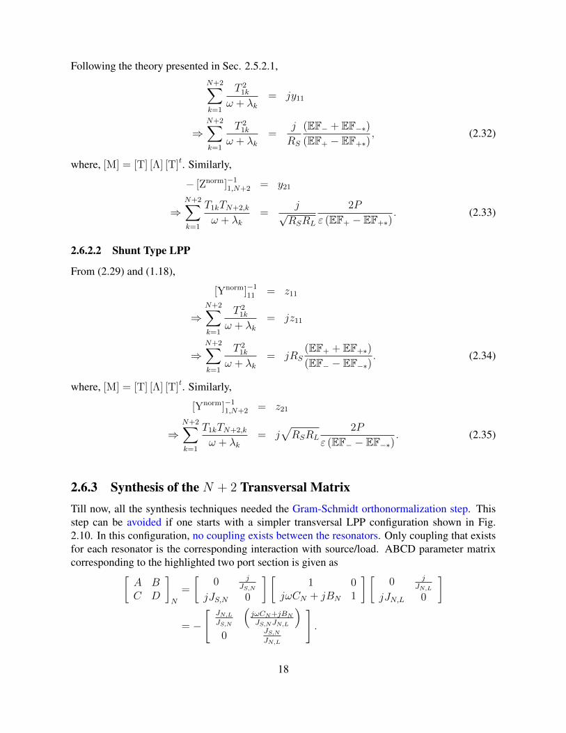
2.6.3 Synthesis of the N + 2 Transversal MatrixTill now, all the synthesis techniques needed the Gram-Schmidt orthonormalization step. Thisstep can be avoided if one starts with a simpler transversal LPP configuration shown in Fig.2.10. In this configuration, no coupling exists between the resonators. Only coupling that existsfor each resonator is the corresponding interaction with source/load. ABCD parameter matrixcorresponding to the highlighted two port section is given as[

A BC D

]N

=

[0 j

JS,N

jJS,N 0

] [1 0

jωCN + jBN 1

] [0 j

JN,L

jJN,L 0

]

= −

[JN,L

JS,N

(jωCN+jBN

JS,NJN,L

)0

JS,NJN,L

].

18

Figure 2.10: Canonical transversal LPP configuration.

Converting ABCD parameters to Y parameters gives[y11 y12y21 y22

]N

=1

b

[d −1−1 a

]=

1

jωCN + jBN

[J

2

S,N JS,NJN,LJS,NJN,L J2

N,L

].

Since all two port sections are connected parallely, overall Y parameter matrix is given as[y11 y12y21 y22

]total

=

[0 j

JS,L

jJS,L 0

]+

N∑k=1

1

jωCk + jBk

[J

2

S,k JS,kJk,LJS,kJk,L J2

k,L

]. (2.36)

From (2.36) and (1.17)

(EF− + EF−∗)RS (EF+ − EF+∗)

=N∑k=1

J2

S,k

jωCk + jBk

and

− 1√RSRL

2P

ε (EF+ − EF+∗)=

j

JS,L+

N∑k=1

JS,kJk,LjωCk + jBk

. (2.37)

So, one can obtain first and last rows (and columns), and all the diagonal elements of (2.30) byequating poles and residues on both sides of (2.37). In addition, all other elements are zero fortransveresal prototype.

19