Paper No. IWC-11-77

Mineral Scale Prediction and Control at Extreme TDS

Robert J. Ferguson

French Creek Software, Inc. Kimberton, PA 19442-0684

IWC-11-77

INTRODUCTION The first scale prediction "index" of note was published by Wilfred F. Langelier in 1936.(1) The Langelier saturation Index (LSI) remains the most used simple index and is applied (and also misapplied) to scale predictions in all areas of water treatment where calcium carbonate scale is of concern. The index was intended for use in the prediction of calcium carbonate scale in municipal water systems. Professor Langelier characterized the applicable systems as a) low ionic strength, b) near neutral pH, and c) ambient temperature. These three parameters where deemed critical to the reliability of prediction due to assumptions made in deriving the index and its subsequent calculation. The limitations of the Langelier Saturation Index and subsequent refined prediction methods can be quantified by reviewing the basis for all of the calcium carbonate prediction methods currently in use, as well as prediction methods for other mineral scales. Overcoming the limitations of this simple index is used in this paper to describe the calculation methods and corrections necessary to calculate scale potential for calcium carbonate, and other mineral scale forming species, under extreme conditions of ionic strength, temperature, and varying composition. In low TDS waters near neutral pH, the assumptions made to simplify calculations to the level of a "slide-rule", are acceptable in many cases. As the ionic strength, temperature, and sometimes pressure of a system increases, more rigorous methods are required to provide reasonably accurate predictions. At extreme TDS, and when a brine composition deviates from a sodium chloride based system, calculations must limit the assumptions if there is to be a reasonable correlation between prediction and real world observation.

All of the indices are derived from the definition of solubility product (Ksp), which can be defined for calcium carbonate as: Equation 1

{Ca}{CO3} = Ksp

where {Ca} is the calcium activity; {CO3} the carbonate activity; Ksp the solubility product.

The solubility product describes the ion activity product expected if a water is in contact with a solid phase of the mineral for an infinite period of time. If the water is left unperturbed, the mineral is expected to dissolve (or precipitate) until the condition that the ion activity product {Ca}{CO3} is equal to the solubility product Ksp. The degree of supersaturation or saturation ratio for a given condition is defined as the ratio of observed Ion Activity Product (IAP) to the Solubility Product: Equation 2 {Ca}{CO3} IAP Saturation Ratio = = Ksp Ksp Scale predictions based upon this relationship are typically expressed either as the Saturation Ratio, or as the log10 of Saturation Ratio. Saturation ratios can be interpreted as outlined in Table 1.

KEYWORDS: scale control, indices, saturation ratio, ion association, speciation, high TDS, scale prediction ABSTRACT Traditional methods for predicting mineral scale deposition and optimizing scale inhibitor dosages are not effective in high ionic strength brines such as shale fracturing flowback fluids. This paper discusses techniques for modeling scale formation and its inhibition in high to extreme TDS brines. The technology discussed is applicable to fracturing operations, produced waters, seawater membrane systems, and zero discharge industrial environments. The advantages and disadvantages of traditional and virial equation approaches are discussed on a practical basis. The thermodynamics and kinetics of mineral scale prediction and dosage optimization are discussed. Implications of open and closed systems, reducing and oxidizing environments are also covered. Authors note: This paper is directed towards engineers and water treatment chemists as a guide for choosing scale prediction methods which are accurate under the conditions they are evaluating, and to assist them in avoiding inapplicable indices such as the use of a simple index like the Langelier Saturation Index in predicting scale in high TDS reverse osmosis brines or extreme TDS flowback systems. It is not intended as a rigorous "how-to" for physical chemists.

IWC-11-77

TABLE 1:

Guidelines for Interpreting Saturation Ratios and Indices

Saturation Ratio (SR) Log10(SR) Scale Prediction

< 1.0 < 0.0 The water is undersaturated. Existing scale will tend to dissolve.

= 1.0 = 0.0 The water is saturated. Scale will not tend to form or dissolve.

> 1.0 > 0.0 The water is supersaturated. Scale will tend to form.

The log10 form and its interpretation should be familiar to users of simple indices such as the Langelier Saturation Index and the Stiff-Davis(2) Index. It can be shown that the simple indices are the log10 of saturation ratio with assumptions that limit their applicability.

Langelier pointed out these assumptions:

Assumption 1: Total Analytical Values Equal Free Ion Concentrations Simple indices are based upon total analytical values for ions such as calcium rather than the "free" concentration of calcium. Ions such as sulfate form complexes with calcium, for example. As a result, indices can be very different for waters with the same ionic strength, and differ only in that one is high in sulfate (which associates strongly) and the other chloride (which tends to remain dissociated and free).

Assumption 2: Carbonate Concentrations Can Be Estimated With Reasonable Accuracy By Assuming That "M" Alkalinity Is Almost Totally Due To Bicarbonate An iterative approach is required to calculate the full distribution of carbonic acid species. The alkalinity used must also be corrected for non-carbonate alkalinity sources such as phosphates, lower carboxylic acids, phosphates, borates, ammonia, silicates, sulfides, cyanide, and other alkalinity sources included in an alkalinity titration.

Assumption 3: Activity Coefficients Can Be Calculated Using Simple Models Early indices such as the LSI used the Debye-Hückel limiting law to estimate the impact of temperature and ionic strength upon activity. In some cases, even ionic strength was estimated using a simple "rule-of-thumb." Assumption 4: pH Is Independent Of Temperature It is common for a sample pH to be analyzed from a cooling tower basin, or at a well head, and then have the

analytical results extrapolated to higher temperatures in a "what-if" scenario. Many of these scenarios have been run using the pH measured in a laboratory environment. Errors introduced by not "correcting" pH to temperature are logarithmic. A 1.0 pH unit error results in up to a ten fold error calcite saturation calculation.

TABLE 2 - SATURATION LEVEL FORMULAS

Calcium carbonate

(Ca)(CO3)

S.L. = _____________ Ksp CaCO3

Barium carbonate

(Ba)(CO3) S.L. = _____________

Ksp BaCO3

Strontium carbonate

(Sr)(CO3) S.L. = _____________

Ksp SrCO3

Calcium sulfate

(Ca)(SO4)

S.L. = ____________ Ksp CaSO4

Barium sulfate

(Ba)(SO4)

S.L. = _____________ Ksp BaSO4

Strontium sulfate

(Sr)(SO4)

S.L. = ____________ Ksp SrSO4

Tricalcium phosphate

(Ca)3(PO4)

2

S.L. = ______________ Ksp Ca3(PO4)2

Amorphous silica

H4SiO4__

S.L. = __________________ (H2O)2 * Ksp SiO2

Calcium fluoride

(Ca)(F)2

S.L. = ___________ Ksp CaF2

Magnesium hydroxide

(Mg)(OH)2

S.L. = _______________ Ksp Mg(OH)2

IWC-11-77

Saturation ratios can be calculated for all common scale forming species and have been found useful in predicting scale applications ranging from low ionic strength potable water, cooling water, oil field brines, and extreme ionic strength flowback brines. Table 2 summarizes the saturation ratio relationship for several common mineral scales. The same relationships are used to predict the amount of preciptation. Equation 1 is modified to calculated the amount of a mineral scale, X, that must dissolve, or precipitate to bring a water to equilibrium. Equation 3: {Ca - X}{CO3 - X} = Ksp

The quantity X is negative when a water is undersaturated, and will indicate the quantity that will dissolve to bring a water to equilibrium. X is positive when supersaturated and represents the quantity that will precipitate to bring a solution to equilibrium. X will be 0 for a saturated solution where the mineral will not dissolve or precipitate. This value is called Calcium Carbonate Precipitation Potential (CCPP) by municipal potable water chemists.(3) and uses the total analytical value and a carbonate estimated using the same assumptions of the LSI. A free ion concentration version is termed momentary excess.(4) Oil field chemists will express this quantity in the units of pounds/1000 barrels. The free ion momentary excess is used to estimate precipitation (or dissolution) for many different scales. Equation 4 represents the quantity X for barite, barium sulfate. Equation 4: {Ba - X}{SO4 - X} = Ksp BaCO3

Momentary excess is reasonably accurate when used to estimate precipitation of scales that are not pH sensitive. It overestimates precipitation for pH sensitive scales like CaCO3, BaCO3, and Ca3(PO4)2. This is due to the decrease in pH that accompanies precipitation of carbonate (or alkaline phosphate) species. An accurate estimation would require an integration of the precipitation from the supersaturated solution pH to the final pH after precipitation to avoid overestimation. Any of the prediction methods can be refined using methods to eliminate, or minimize the impact from the assumptions made with simple indices. ION ASSOCIATION (Minimizing Assumption 1) Ions in solution are not all present as the free species. For example, calcium in water is not all present as free Ca+2. Other species form which are not available as driving forces for scale formation. Examples include the soluble calcium sulfate species, hydroxide species, and

bicarbonate - carbonates. Table 3 outlines example species that can be present in a typical water. The use of ion pairing to estimate the free concentrations of reactants overcomes several of the major shortcomings of traditional indices. Indices such as the LSI correct activity coefficients for ionic strength based upon the total dissolved solids. They do not account for "common ion" effects.(5) Common ion effects increase the apparent solubility of a compound by reducing the concentration of reactants available. A common example is sulfate reducing the available calcium in a water and increasing the apparent solubility of calcium carbonate. The use of indices which do not account for ion pairing can be misleading when comparing waters where the TDS is composed of ions which pair with the reactants versus ions which have less interaction with them.

When indices are used to establish operating limits such as maximum recovery in reverse osmosis systems, maximum cycles of concentration in cooling water, optimum blend ratios, or maximum pH, the differences between the use of indices calculated using ion pairing can be of extreme economic significance(6). In the best case, a system is not operated at as high a recovery or as high a concentration ratio as possible, because the use of indices based upon total analytical values resulted in high estimates of the driving force for a scalant. In the worst case, the use of indices based upon total ions present can result in the establishment of operating limits being too high. This can occur when experience on a system with high TDS water is translated to a system operating with a lower TDS water. The high indices which were found acceptable in the high TDS water may be unrealistic when translated to a water where ion pairing is less significant in reducing the apparent driving force for scale formation.

Figure 1 compares the impact of sulfate and chloride on scale potential. The curves profile the calculation of the Langelier Saturation Index in the presence of high TDS. In one case the TDS is predominantly from a high chloride water. In the other case, a high sulfate water is profiled. Profiles for the index, calculated based upon total analytical values, are compared with those calculated with ion association model free ion activities. Table 3 compares the calcite saturation ratios for two similar waters with the LSI for both. The waters were of a simulated composition for this example. A water composed of 1000 mg/L of calcium and 120 mg/L "M" alkalinity was balanced with chloride in water 1, and sulfate in water 2. Ion association model calcite saturation ratios, and the simple LSI were calculated for both and compared. The purpose was to show the impact of not accounting for ion pairing by using a simple index rather

IWC-11-77

than a method incorporating ion association and speciation.

The simulation demonstrates that the Langelier Saturation Index, is not significantly different when the primary anion in a water is chloride, which is almost totally ionized and free, versus sulfate, which is highly associated. The calcite saturation ratio calculated using an ion association model with full correction changes significantly. The "Free" calcium values demonstrate the increased association due to sulfate versus chloride.

The practical significance of the illustration is that ion pairing and a full calculation of species should be used to calculate free ion concentrations when indices are to be used as a general rule, for establishing control limits in a cooling system or reverse osmosis, or as a driving force for dosage optimization. This assures that the index means the same in widely varying waters. A practical corollary is that simple indices should be correlated to each individual water to which they are applied, but that the results observed in one water can be extrapolated to others when ion association model indices are used. For example, the scale inhibitor HEDP (1-1 hydroxyethylidene diphosphonic acid) has an upper limit of 150 saturation ratio.(6,7) This equates to LSI limits of 2.5 in a high sulfate cooling water but 2.8 in a high chloride water. In both cases, the upper limit is 150 calcite saturation ratio when calculated using an ion association model with full speciation, including the appropriate corrections for non-carbonate alkalinity. Speciation of a water is time prohibitive without the use of a computer for the iterative number crunching required.

The process is iterative and involves:

1. Checking the water for electroneutrality via a cation-anion balance, and balancing with an appropriate ion (e.g sodium or potassium for cation deficient waters, sulfate, chloride, or nitrate for anion deficient waters).

2. Estimating ionic strength, calculating and correcting activity coefficients and dissociation constants for temperature, correcting alkalinity for non-carbonate alkalinity.

3. Iteratively calculating the distribution of species in the water from dissociation constants (a partial listing of equations is outlined in Table 4).

4. Checking the water for balance and adjusting ion concentrations to agree with analytical values.

5. Repeating the process until corrections are insignificant.

6. Calculating saturation levels based upon the free concentrations of ions estimated using the ion association model (ion pairing).

Table 4: Example Ion Pairs Used To Estimate Free Ion Concentrations

CALCIUM [Calcium] = [Ca+II] + [CaSO4] + [CaHCO3

+I] + [CaCO3] + [Ca(OH)+I] + [CaHPO4] + [CaPO4

-I] + [CaH2PO4+I]

MAGNESIUM [Magnesium] = [Mg+II] + [MgSO4] + [MgHCO3

+I] + [MgCO3] + [Mg(OH)+I] + [MgHPO4] + [MgPO4

-I]+[MgH2PO4+I]+[MgF+I]

BARIUM [Barium] = [Ba+II] + [BaSO4] + [BaHCO3

+I] + [BaCO3] + [Ba(OH)+I] STRONTIUM [Strontium] = [Sr+II] + [SrSO4] + [SrHCO3

+I] + [SrCO3] + [Sr(OH)+I] SODIUM [Sodium] = [Na+I] + [NaSO4

-I] + [Na2SO4] + [NaHCO3] + [NaCO3-I]

+ [Na2CO3] + [NaCl]+[NaHPO4-I]

POTASSIUM [Potassium] = [K+I] +[KSO4

-I] + [KHPO4-I] + [KCl]

IRON [Iron] = [Fe+II] + [Fe+III] + [Fe(OH)+I] + [Fe(OH)+II] + [Fe(OH)3

-I] + [FeHPO4+I] + [FeHPO4] + [FeCl+II] + [FeCl2

+I] + [FeCl3] + [FeSO4] + [FeSO4

+I] + [FeH2PO4+I] + [Fe(OH)2

+I] + [Fe(OH)3] + [Fe(OH)4

-I] + [Fe(OH)2] + [FeH2PO4+II]

ALUMINUM [Aluminum] = [Al+III] + [Al(OH)+II] + [Al(OH)2

+I] + [Al(OH)4-I]

+ [AlF+II] + [AlF2+I] + [AlF3] + [AlF4

-I] + [AlSO4+I]

+ [Al(SO4)2-I]

Total Analytical Value Free Ion Concentration

IWC-11-77

The use of full speciation and calculation of scale saturation ratios or indices based upon "free ion" concentrations rather than total analytical values, expands the applicability of scale potential calculations to seawater concentrations and above in sodium chloride based systems. Using "free ion" concentrations for calculations is a major step in overcoming the deficiencies of the simple indices, and extending the useful range for scale prediction to seawater and beyond. Ion association model speciation is combined with other techniques to further refine scale prediction at high TDS. RIGOROUS CARBONIC ACID CALCULATIONS (Minimizing Assumption 2) There are two assumptions made in simple indices concerning the calculation of carbonic acid species distribution and the carbonate concentration used for calcium carbonate scale indices:

1) There is no need to correct alkalinity for non-carbonate alkalinity. In other words, all of the alkalinity titrated in an "M" alkalinity titration is from carbonic acid species.

2) You can assume that the alkalinity is predominantly bicarbonate, and that the error in calculating carbonate based upon this assumption is negligible.

As pointed out by Professor Langelier in 1936,(1) the errors introduced by these assumptions is alkalinity source other than hydroxide in a water. The assumptions are not warranted when the pH is higher than neutral, and when non-carbonate alkalinity sources such as phosphates, silicates, ammonia, and sulfides are present.

It is important to remember that a total "M" alkalinity titration measures the acid neutralizing capacity of the water, not just the carbonate and bicarbonate contributions.(8)

In neutral waters where carbonic acid equilibria is in complete control, simple indices such as the Langelier saturation index have their minimum error. In this case:

Equation 5 ANC = 2.0 * [CO3

=] + [HCO3-] +[OH-] - [H+]

The contribution of hydroxide to the Acid Neutralizing Capacity is negligible near pH 7. Carbonate and bicarbonate concentrations can be estimated with reasonable accuracy. At higher pH, or when other alkalis such as ammonia are present: Equation 6 ANC = 2.0 * [CO3

=] + [HCO3-] +[NH3]

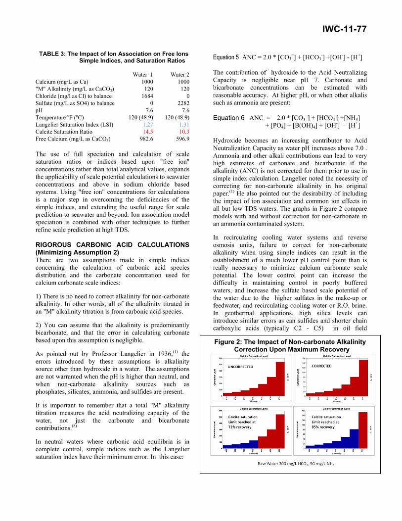
+ [PO4] + [B(OH)4] + [OH-] - [H+] Hydroxide becomes an increasing contributor to Acid Neutralization Capacity as water pH increases above 7.0 . Ammonia and other alkali contributions can lead to very high estimates of carbonate and bicarbonate if the alkalinity (ANC) is not corrected for them prior to use in simple index calculation. Langelier noted the necessity of correcting for non-carbonate alkalinity in his original paper.(1) He also pointed out the desirability of including the impact of ion association and common ion effects in all but low TDS waters. The graphs in Figure 2 compare models with and without correction for non-carbonate in an ammonia contaminated system.

In recirculating cooling water systems and reverse osmosis units, failure to correct for non-carbonate alkalinity when using simple indices can result in the establishment of a much lower pH control point than is really necessary to minimize calcium carbonate scale potential. The lower control point can increase the difficulty in maintaining control in poorly buffered waters, and increase the sulfate based scale potential of the water due to the higher sulfates in the make-up or feedwater, and recirculating cooling water or R.O. brine. In geothermal applications, high silica levels can introduce similar errors as can sulfides and shorter chain carboxylic acids (typically C2 - C5) in oil field

TABLE 3: The Impact of Ion Association on Free Ions Simple Indices, and Saturation Ratios

Water 1 Water 2 Calcium (mg/L as Ca) 1000 1000 "M" Alkalinity (mg/L as CaCO3) 120 120 Chloride (mg/l as Cl) to balance 1684 0 Sulfate (mg/L as SO4) to balance 0 2282 pH 7.6 7.6 Temperature oF (oC) 120 (48.9) 120 (48.9) Langelier Saturation Index (LSI) 1.27 1.31 Calcite Saturation Ratio 14.5 10.3 Free Calcium (mg/L as CaCO3) 982.6 596.9

Figure 2: The Impact of Non-carbonate Alkalinity Correction Upon Maximum Recovery

IWC-11-77

chemistry. Higher treatment rates than necessary can also result from a failure to correct for non-carbonate alkalinity. Ion association model saturation levels corrects for the errors introduced by non-carbonate alkalinity and high TDS and should be employed when available.(5) ACTIVITY COEFICIENTS CALCULATION (Minimizing Assumption 3) Ions in water have a decrease in their energy as ionic strength increases. In very dilute solutions, the predominant effect causing a decrease in activity is the long range repulsion between same charge molecules and the attraction between oppositely charged molecules. As ionic strength increases, the molecules become closer, and their hydration layers begin to interact, adding a short range factor for repulsion and attraction. At extreme concentrations, only a few water of hydration molecules separate ions, and the short range effects become extremely significant. At the extreme ionic strength (above about 6 molal), the activity of water also decreases significantly as water molecules increasingly become tied up in hydration layers around molecules. (9) So there are several levels of ion interactions that can decrease the available energy for reaction. This decrease in energy is modeled using an activity coefficient. Two basic approaches are used to model activity coefficients and are discussed in this section of the paper: those derived from the Debye - Hückel equations, (10) and those that are extended to refine the short term interactions using virial expansions, in the form of the Pitzer or equivalent equations. (11) Debye - Hückel Activity Coeficients The first indices used activity corrections based upon the Debye - Hückel limiting law (Equation 7), and were applicable to only the most dilute solutions. This is the activity model that was used in the original Langelier Saturation Index.

Equation 7 log ƴi = - A zi2 √I

where A is a temperature dependent constant (0.5092 at 25oC) z is the ions electrical charge (e.g. +1 for Na) I is the solution ionic strength I = ½ ∑ mi zi

2 mi is the molality Robinson and Stokes worked with the Debye-Hückel method for activity coefficients and published the most

common method for estimating the long range effect of charge interactions, the Debye-Hückel equation. (12)

A zi2 √I

Equation 8 log ƴi = -

1 + åi B √I where A is a temperature dependent constant (0.5092 at 25oC) B is a temperature dependent constant (0.3283 at 25oC) z is the ions electrical charge (e.g. +1 for Na) I is the solution ionic strength å      is an empirical ion size mi is the molality

Davies published a useful variant in 1962 that includes an adjustment factor to compensate for the short range interactions. (13)

√I Equation 9 log ƴi = - A zi

2 - 0.3 I

1 + √I Helgeson (1969) introduced a most useful derivation of the Debye-Hückel and Davies equations that incorporates an ion specific adjustment for the impact of higher ionic strength and long range interactions:

A zi2 √I

Equation 10 log ƴi = - + Ḃ I

1 + åi B √I where Ḃ    is a temperature dependent        adjustment parameter. The Helgeson extension is used in geochemical models and is commonly called the B-dot equation. It is reportedly useful to 3 molal ionic strength in NaCl based systems and up to 1 molal in other solutions. Ḃ  values have been published  in  the  temperature range of 0 oC to 300 oC. (14,15)

IWC-11-77

32 62 92 122 152 182 212

12

12.5

13

13.5

14

14.5

15

0 20 40 60 80 100

Temperature (°F)

pKw

Temperature (°C)

pKw versus Temperature

The combination of the B-dot equation format and a full speciation using an ion association model is perhaps the most commonly used method for scale prediction and refined index calculation in low to the lower high end of ionic strength brines. The combination has been used successfully in the 3 to 6 molal range for NaCl based brines. Further refinements are desirable in even higher TDS brines. Virial Expansion Activity Models Coefficients for the Debye-Hückel derived activity coefficient models have primarily been derived in NaCl based systems. When dealing with other brines, such as NaBr based completion fluids, other methods are more appropriate. These methods start with a Debye-Hückel based factor for long term interactions, and expand it to model the short term interactions of ions. The virial methods typically lump the ion association effects into the overall model and are most useful in extreme TDS brines, and high to extreme non-NaCl based brines. (17,18)

The derivation of the virial expansion method is beyond the scope of this paper. Scale prediction software based upon virial methods typically include the two types of virial models: (Pitzer and the Havey-Moller-Weare approach). Pitzer based models lump speciation effects into the ion interaction factors. The author prefers complete ion association models or "hybrid" Pitzer based paradigms in lower TDS systems. pH VARIATION WITH TEMPERATURE (Minimizing Assumption 4) "What-if Scenario" modeling has been commonplace in water treatment. A water treatment chemist will profile a given water chemistry over the complete range of temperature expected to determine what types of scale might be expected at different points in a system. The coldest point might be of interest for scales like amorphous silica and barium sulfate which are least soluble at the coldest point in the system. Or they might

find the hottest point to be of interest for the inversely soluble calcium carbonate. Many of these "what-if" extrapolations use the pH that was supplied with the analysis, and do not adjust the pH used to the temperature evaluated. There are two kinds of temperature affects that might create confusion. The first effect is equipment related due to electronics and probe compensation. pH meters proclaim "automatic temperature correction." This covers the measurement corrections which have become invisible to the field engineer. Algorithms are included to correct the electronics for measurement at temperatures other than 25 oC. The second type of correction needed is for the variation of pH with temperature due to the variation of Kw, the dissociation constant for water, with temperature. As a result, the pH for pure water also changes. Figure 3 depicts the variation of pKw with temperature, while Figure 4 profiles the pH of pure water at atmospheric pressure versus temperature. pH is corrected to the temperature evaluated by taking advantage of conservation of alkalinity. The pH is calculated such that the alkalinity is maintained as temperature changes. (20,21) Tables 5 and 6 compare a water analysis profile versus temperature calculated with and without correction for pH change with temperature. It is of increasing importance to correct pH for temperature as the pH at 25oC increases above pH 8.6 . Alkalinity can increase wildly if the pH is not corrected, resulting in erroneous predictions of high pH scale formation, and erroneous ion pairing values for hydroxide species. If you have a pH measured at the temperature you are evaluating, use it. If the pH was measured at a different temperature, use software that corrects pH from the temperature at which it was measured to the temperature being evaluated.

Figure 4 Figure 3

IWC-11-77

SCALE INHIBITION UNDER EXTREME STRESS Scale inhibitor dosage modeling allows calculation of the minimum effective scale inhibitor dosage. Models typically include a function of a driving force for mineral scale formation, temperature as it affects rate. A critical parameter is the induction time extension needed to allow a treated water to safely pass through a system before the onset of precipitation, or growth on an existing substrate. The models used in industrial cooling water, oil field brines, and reverse osmosis systems have been well documented. (6,7,,14,18,19) Induction time extension is the key to the models. Reactions do not occur instantaneously. A time delay occurs once all of the reactants have been added together. They must come together in the reaction media to allow the reaction to happen. The time required before a reaction begins is termed the induction time. Thermodynamic evaluations of a water scale potential, predict what will happen if a water is allowed to sit undisturbed, under the same conditions, for an infinite period of time. Even simplified indices of scale potential, such as the ion association model saturation index, can be interpreted in terms of the kinetics of scale formation. For example, calcium carbonate scale formation would not beexpected in an operating system when the saturation

index for the system only slightly above 1.0 x saturation. The driving force for scale formation is too low for scale formation to occur in finite, practical system residence times. Scale would be expected if the same system operated with a saturation index of 50. The driving force for scale formation in this case is high enough, and induction time short enough, to allow scale formation in even the shortest residence time industrial systems. (18) "Scale inhibitors don't prevent precipitation, they delay the inevitable by extending induction time." (6,7,14,18,19)

Equation 11 1 Induction Time = _____________________________ k [Saturation Ratio - 1]P-1 Where: Induction Time is the time before crystal formation and growth occurs; k is a temperature dependent constant; Saturation Ratio is the degree of supersaturation; P is the critical number of molecules in a cluster prior to phase change

Table 5 pH Adjusts to Maintain Alkalinity as Temperature Increases 77oF (25oC) 100oF(37.7oC) 200oF (93.3oC) 300oF (149 oC) 400oF (204 oC) Calcium (as CaCO3) 123 123 123 123 123Magnesium (as CaCO3) 34 34 34 34 34Sodium (as Na) 18 18 18 18 18Chloride (as Cl) 34 34 34 34 34Sulfate (as SO4) 23 23 23 23 23"M" Alkalinity (as CaCO3) 125 125 125 125 125Bicarbonate (as HCO3) 150.9 150.8 147.6 142.6 136.8Carbonate (as CO3) 0.7 0.9 2.2 4.1 6.6Hydroxide (as OH) 0.1 0.1 0.4 1.1 1.6pH (at temperature) 7.58 7.51 7.22 6.96 6.75Pressure (psi) 14.7 14.7 14.7 67.0 247.

Table 6 pH Maintained as Temperature Increases 77oF (25oC) 100oF(37.7oC) 200oF (93.3 oC) 300oF (149 oC) 400oF (204 oC) Calcium (as CaCO3) 123 123 123 123 123Magnesium (as CaCO3) 34 34 34 34 34Sodium (as Na) 18 18 18 18 18Chloride (as Cl) 34 34 34 34 34Sulfate (as SO4) 23 23 23 23 23"M" Alkalinity (as CaCO3) 125 126 130 142 162Bicarbonate (as HCO3) 150.9 151.0 147.1 137.0 120.8Carbonate (as CO3) 0.7 1.1 4.9 14.9 30.8Hydroxide (as OH) 0.1 0.9 0.4 4.7 11.0pH (as measured at 25oC) 7.58 7.58 7.58 7.58 7.58Pressure (psi) 14.7 14.7 14.7 67.0 247.

IWC-11-77

Temperature is a second parameter affecting dosage and is represented by the temperature dependent constant k in Equation 11. A common concept in basic chemistry is that reaction rates increase with temperature. The rule-of-thumb frequently referenced is that rates approximately double for every ten degree centigrade increase in temperature. The temperature constant above was found to correlate well with the Arrhenius relationship, as outlined in Equation 12.

Equation 12 -Ea/RT k = A e Where: k is a temperature dependent constant; Ea is activation energy; R is the Gas Constant; T is absolute temperature.

Models for optimizing dosage demonstrate the impact of dosage on increasing induction time. An example is profiled in Figure 3. Saturation level and temperature impacts upon the dosage requirement to extend induction time are depicted in figures 4 and 5. Factors impacting the antiscalant dosage required to prevent precipitation are summarized as follows: Time The time selected is the residence time the inhibited water will be in the cooling system. The inhibitor must prevent scale formation or growth until the water has passed through the system and been discharged. Figure 6 profiles the impact of induction time upon dosage with all other parameters held constant.

Degree of Supersaturation An ion association model saturation level is the driving force for the model outlined in this paper, although other, similar driving forces have been used. Calculation of driving force requires a complete water analysis, and the temperature at which the driving force should be calculated. Figure 7 profiles the impact of saturation level upon dosage, all other parameters being constant.

Temperature Temperature affects the rate constant for the induction time relationship. As in any kinetic formula, the temperature has a great impact upon the collision frequency of the reactants. This temperature effect is independent of the effect of temperature upon saturation level calculations. Figure 8 profiles the impact of temperature upon dosage with other critical parameters held constant.

pH pH affects the saturation level calculations, but it also may affect the dissociation state and stereochemistry of the inhibitors.(14,18) Inhibitor effectiveness can be a function of pH due to its impact upon the charge and shape of an inhibitor molecule. This effect may not always be significant in the pH range of interest (e.g. 6.5 to 9.5 for cooling water).

The same models work well under extreme conditions. Two additional parameters must be taken into account at the extremes: inhibitor dissociation and active state, and stereochemistry at high ionic strength or pH extremes. Active sites "It is easier to keep a clean system clean than it is to keep a dirty system from getting dirtier." This rule of thumb may well be related to the number of active sites for growth in a system. When active sites are available, scale forming species can skip the crystal formation stage and proceed directly to crystal growth.

IWC-11-77

Equation 13 adds the impact of inhibitor dosage on extending induction time to Equation 11. The goal of the inhibitor dosage is to extend the time before precipitation until the treated water has passed through the system and precipitation will no longer be a threat to the system. Equation 13

[inhibitor]M Induction Time = _____________________________ k [Saturation Ratio - 1]P-1

Other factors can impact dosage such as suspended solids in the water. Suspended solids can act as sources of active sites, and can reduce the effective inhibitor concentration in a water by adsorption of the inhibitor. State-of-the-art modeling software incorporates the ability to optimize dosages for all of the scales expected. Scale inhibitors have upper limits and are not effective above saturation level driving force, regardless of the inhibitor dosage. (14,18) Table 7 outlines generally accepted limits for inhibition of scales by standard commercially available inhibitors. Limits are provided for both standard inhibitors and for those formulated for extreme, "stressed" conditions.(21)

In summary, scale inhibitor dosages under extreme conditions should:

1) use a driving force appropriate to the ionic strength and brine type for model development. e.g. A Langelier

Saturation Index based model would not be appropriate to R.O. concentrate or recirculating cooling water at pH 8.6 ,

2) correct for pH effects on the inhibitor dissociation form and activity.

3) avoid using incompatible inhibitors. e.g. Do not use iron sensitive phosphonates in high iron flowback systems. 4) include a realistic limit. Assure that the point where an inhibitor will fail regardless of dosage is known. SUMMARY AND RECOMMENDATIONS Scale prediction methods have advanced significantly since the first practical method, the Langelier Saturation Index, was published in 1936. Advances in electrolyte chemistry modeling, and computer calculation capabilities, have eliminated the need for the assumptions inherent in the simple indices, or limited them to a negligible impact. Scale prediction methods should be chosen for the range of data based upon ionic strength and type of system (e.g. NaCl).

Simple indices such as the Langelier Saturation Index, should only be used for very dilute waters near neutral pH, and then only when more advanced models are not available. Professor Langelier outlined a wish list of assumptions necessary to allow calculations in a reasonable time in 1936. Personal computers and advances in data for electrolytes have fulfilled Dr. Langelier's wish list and limited, or eliminated, the need for these critical assumptions.

TABLE 7: TREATED LIMITS COMPARISON

SCALE FORMING SPECIE

FORMULA

MINERAL NAME

TYPICAL SATURATION RATIO LIMIT

STRESSED TREATMENT LIMIT

Calcium carbonate CaCO3 Calcite 135 - 150 200 - 225

Calcium sulfate CaSO4*2H2O Gypsum 2.5 - 4.0 4.0 +

Barium sulfate BaSO4 Barite 80 80+

Strontium sulfate SrSO4 Celestite 12 12

Silica SiO2 Amorphous silica 1.2 2.5

Tricalcium phosphate Ca3(PO4)2 1500 - 2500 125,000

IWC-11-77

REFERENCES 1 Langelier, W.F.(1936),The Analytical Control Of

Anti-Corrosion Water Treatment, JAWWA, Vol. 28, No. 10, 1500-1521.

2 Stiff, Jr., H.A., Davis, L.E.(1952), A Method For Predicting The Tendency of Oil Field Water to Deposit Calcium Carbonate, Pet. Trans. AIME 195;213.

3 Rossum, J. R. , Merrill, D.T. (1983), An Evaluation of the Calcium Carbonate Saturation Indexes, .Journal of the American Water Works Association 75: 95–100.

4 Ferguson, R.J.,(1982),A Kinetic Model for Calcium Carbonate Scale, NACE..

5 Ferguson, Robert J.,(1992) Computerized Ion Association Model Profiles Complete Range of Cooling Water Parameters, International Water Conference.

6 Ferguson, R.J., Ferguson, B.R, Stancavage, R.F. (2011), Modeling Scale Formation and Optimizing Scale Inhibitor Dosages in Membrane Systems, AWWA Membrane Technology Conference.

7 Ferguson, R.J.(1992), Developing Scale Inhibitor Models, WATERTECH, Houston, TX.

8 Stumm, W., Morgan, J.J. (1996) Aquatic Chemistry, John Wiley & Sons, Inc,, New York, pp 138 - 140.

9 Bethke,C.M.(2008), Geochemical and Biogeo- chemical Reaction Modeling, Cambridge Press, pp 115-117.

10 Bethke,C.M.(2008),pp 123-127 11 Zemaitis J.F., Clark, D.M., Rafal, M., Scrivner, N.C.

(1986), Handbook of Aqueous Electrolytee Thermodynamics, AIChE, pp 47-66.

12 Robinson, R.A., Stokes, R.H. (2002) Electrolyte Solutions, Dover Publications, pp 229-233.

13 Bethke,C.M.(2008),pp 118-119 14 Tomson, M.B., Fu, G., Watson, M.A. Kan, A.T. (2002),

Mechanisms of Mineral Scale Inhibition, Society of Petroleum Engineers, Oilfield Scale Symposium, Aberdeen, UK

15 Helgeson, H.C. (1969), Thermodynamics of Hydrothermal Systems at Elevated Temperatures and Pressures, American Journal of Sciences, 267, 729 – 804.

16 Bethke,C.M.(2008), pp 127-130. 17 Zemaitis J.F. (1986), pp 71-76. 18 Ferguson, R. (2011),Thermodynamics and Kinetics of

Cooling Water Treatment, Association of Water Technologies.

19 Ferguson, R.J., Weintritt, D. (1994), Developing Scale Inhibitor Models for Oil Field Applications, National Association of Corrosion Engineers.

20 Langelier, W.F. (1946), Effect Of Temperature On The pH Of Natural Waters, JAWWA, Vol. 38:179, 1946.

21 Ferguson, R.J. (2004), Water Treatment Rules of Thumb: Fact or Myth, Association of Water Technologies.