Modal Parameter Estimation: A Unified Matrix Polynomial Approach

Randall J. Allemang, PhD

Professor David L Hrown, PhD

Professor William Fladung

Research Assistant

Structural Dynamics Research I "aboratory Department of Mechanical. Industrial and N udcar Engmccring

University of Cincinnati

Cincinnati, Ohio 4-"221-0072 U.S. A.

ARSTRACT

As many different modal parameter estimation algorithms have evolved over the past twenty years, the ability to view all algorithms from a unified perspective becomes important in order to compare and contrast the numerical characteristics of each algoritlun. An approach that

recognizes the underlying matrix polynomial structme of the numerical algorithms is one approach that achieves this goal. The fnl\nwing development serves a<; a framework to most modal parameter estimation algorithms that have been documented in the literature. Tht: overall approach is given as wdl a.<> the fundamental or basic equation fonnulation for each method. While there arc many implementations of these algorithms in use, that may or may not utilize the theoretical approach given here, the ability to view each method in a conunun framework allows the numerical characteristics of each algorithm to be identified a." advantages and disadvantages of the various methods.

Note that the practical or commercial implementation of these algorithms may be presenteU differently elsewhere in order to reflect the spe­cific numerical solution utilized.

1. Introduction

Modal parameter estimation is a special case of system identifica­tion where the a priori model nf the system is known to he in the funn of modal parameters. ( lver the past twenty years, a number

of algorithms have been develnpeU to estimate modal parameters from measured frequency or impulse response function Uata.

Modal Parameter Estimation Algorithms

CEA Complex Exponential Algorithm P-21

LSCE I ,ea.<;t Squares Complex Exponential [1.2]

PTll Polyreference Time J)omain [30,31]

lTD Ibrahim Time Domain 19 -121

MRITD Multiple Reference Ibrahim Time I )omain [9[

ERA Eigensystem Realization Algorithm [l:"\,2:"1]

PFD Polyreferencc Frequency Domain rg,1~-21.24.33J

SFD Simultaneous Frequem:y Domain Pl

MRFD Multi-Reference Frequency Domain [4[

RFP Rational Fraction Polynomial 1281

OP Orthogonal Polynomial 125.26.2~1

CMIF Complex Mode Indication Function [26)

1:"-BLE 1. Acronyms- Modal Parameter Estimation Algorithms

While must of these individual algonthms. summarized in Table I and 2. ,u-c well undcrstoud. the comparison of one algmithm to another has become one of the thrusts nf current research in this Jrca. Comparison of the different al~mithms is possible when the

algmithms are refonnulated using a corrunon mathmatical struc­

ture. This reformulation attempts to characterize different classes of modal parameter estimation techniques in terms of the structure of the underlying matrix polynomials rather than the phys1cally based models useU historically. Since the modal parameter estima­

tion process involves a greatly over-determined problem (mme data than independent equations). this refonnulation is helpful 111

understandmg the different numerical characteristics tlf each algo­rithm and, therefore, the slightly different estimates of modal parameters that each algorithm yields. As a part nf this refonnula­

tion of the algorithms, this work ha." focussed on the development of a conceptual understanding of modal parameter estimation tech­nology. This understanUing involves the ability to conceptualize the measured data in terms of the concept of Chamcteri.Hic s·pace. the data domain (time. frequency, spatial), the evaluation nf the order of the problem, the condensatiun of the data. anU a conmwn parameter estimation theory that can serve <L" the hasis for develop­mg. any of the algorithms in use today. The following sections will review these concepts as applied to the current modal p.trameter estimation metbotlology.

2. Definition: Modal Parameters

Modal identification involves estimating the modal parameters of a structural system from measureU input-output data. Most cum~nt modal parameter estimation is ba.-.ed upon the measured data heing the fn:quency response function or the equivalent impulse resptlllSC function. typically fouml hy inverse Fourier transfonnin,? the fre­

quency response function. Modal parameters include the complex-

501

( )utput I)( )r

Input DOF

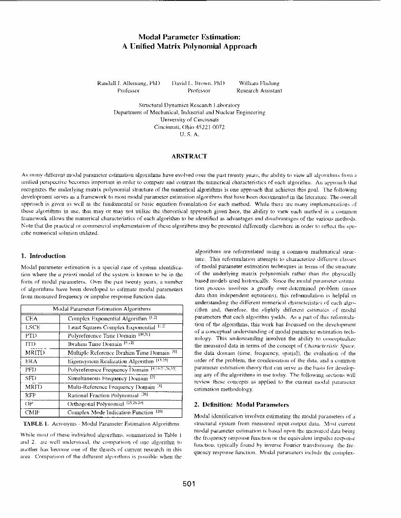
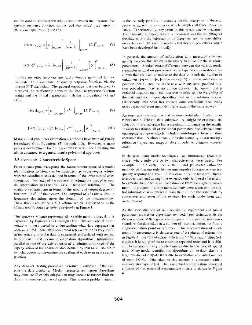
Figure 1. Conceptualization of Modal Characteristic Space

valued modal frequencies (A,), modal vectors ({IfF,}) and modal scaling (modal mass or modal A). Additionally, most current algo­rithms estimate modal participation vectors ({ L,}) and residue vec­tors ({A,}) a.·.; part of the overall process.

Modal participation vectors are a result of multiple rc!Crence modal parameter estimation algorithms and define how each modal vedor is excited from each of the reference locations induded in the measured data. The combination of the modal participation vector ({ Lr}) and tbe modal vector ({IfF,}) for a given mode give the residue matrix (A1"i,:::: Lqr'l'pr) for that mode. In general. these two vectors represent portions of the right and left eigenvectors asso(.'iat~d with the structural system for that specific mmlc of vibration. Normally, the system can he assumeJ to be reciprocal ami the right and left eigenvedors. and tht:refore the modal partici­patinn vector and the modal vector. will he proportional to lllle another. Under this assumptton, the modal participation vector can he used in a weighted least squares error solution procedure to esti­mate the mudal vectors in the presence of multiple references. The­oretically. for reciprocal systems. these modal participation factors should be in proportion to the modal coefficients of the reference degrees of freedom for each modal vector.

In general. modal parameters are considered global pmperties uf the system. The concept of global mmlal parameters simply means that there is only one answer for each modal parameter and that the modal par~uneter estimation solutinn procedure enforces this con­straint Every frequency response nr impulse rt---sponse function measurement theoretically contains the infnrmation that is repre­<;entcd hy the charactenstJc equation, !he modal frequencies ami Liampmg. If mdividual measurements are treated in the solution procedure independem of (me another. the S!dution procedure docs not guarantee thai a -"Ingle set of modal frequencies and dampmg wdl be generated. In likewJsc manner. if more thaTl nnL: n:ferenn.' is mea:-.ured Ill the data sd, redundant eslimares (lf the modal

vectms can he estlln<1ted unless th!..-' S!dlltlon pn1cedure utililt''- ,dl references in the estimatinn pruccss simultant:nllsly. Most tlf the current modal parameter estimatinn algorithm . ..; estimate the modal fr!..-'4uencies and d;unpin~ in a glnhal s.:nsc hut vc1 y few estimalc the modal vedors 111 a global s!..-'nsc by enfurcing the renpwcity

constraint.

3. Modal Identification Concepts

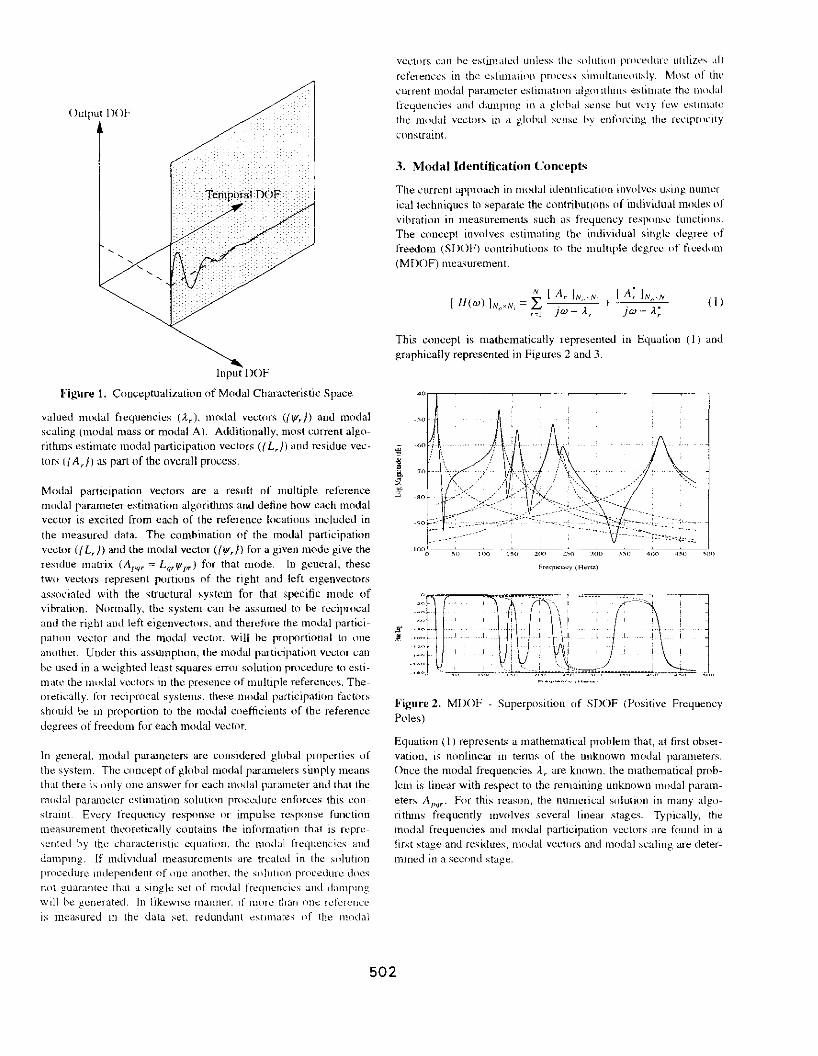
The current approach in modal identification invulvcs using numer­ical techniques to separate the contributions uf individual modes of vibration in measurements such as frequency response functions. The concept involves estimating the individual single degree of freedom (SDOF) t:ontributions to the multiple degree of fr!..-'edum (MDOF) mca<;urcment.

N

[ H(w) IN0,N, = L (I)

,-1

This concept is mathematically represented in Equation ( 1) and graphically represented in Figures 2 and 3.

"" --~0

w ~

~ :t ;o

3 '"

Figure 2. MDOF - Superposition of SDOF (Positive Frequency Poles)

Equation (1) represents a mathematical problem that, at first obser­vation, is nonlinear in terms of the unknown modal parameters. Once the modal frequencies II., arc known. the mathematical prnh­lcm is linear with respect to the remaining unknown modal param­eters Apqr· For this reason, the numeri!..-'al solution in many algo­nthms frequently mvolves several linear stage.'-'. Typically, the modal fn:t.juencies and modal participation vectors are found in a first stage and residues, modal vectors and modal scaling arc deter­mmed in a second stage.

502

40 r

"I

j ' ·v ~ ~

-70 r ~

~ "or

1 -40 ~

~------

-lOr! .c-----

0 "' j()(J ]~0 100 l~O 4f)() 45(> 50()

F<e'luency (H.,.rtz)

·_--·-·f_·--~:_r· '.\u· , ~~ .. _ , , 'J 1_, Lt;·· : -_·iriN- ~---·-·· ·J· --y ! ! ' ~ ;' ·- __ t\=-"·-~- \_ __

Figure 3. MDOF Superposition of SDOF (Positive Negative Frequency Poles)

3.1 Concept: Model Order Relationships

The estimation nf an appropriate model order is the most important problem encounteretl in modal parameter estimation. This prob­lem is complicated due to the formulation of the parameter estima­tion model in the time or frequency domain. due to a single or mul­tiple reference formulation of the modal parameter estimation mudd. and the effects of random and hias errors on the modal parameter estimation model. The basis of the formuhltinn of the correct model order can he seen by expanding the second order matrix (N x N) equation of motion to a higher order model (2N).

This ts a necessary process required to handle the case where the spatial information (measured degrees of freedom) is truncated to a stze smaller than the number of modal frequencies in the measureti data. There arc several ways that this concept can he developed.

Om:: method is to start with the steady-state matrix equ<ltion of motion and. for example. Lapla~..~e transform this equation tn the s d(Jmain.

[ IM Is'+ IC I'+ [K I] IX(sl I~ {F(sl I (2)

The above matrix equation yields a charadcristic matrix polyno­

mial equation in the following form:

(3)

This characteristic cquatinn is a matrix polynomial of second order which can he further partitioned as follows:

[M11J IM,,I [M, I [M,,I

s: +

IM,11i IMnnJ

[C, I [Crnl

1 IC, I [C,,I

Is+ [C,, I fCnnl j

[K, I [K,,[ IK, I [K,,I

0 (4)

[K,,[ [K,.,,]

This partitioned equation can he expanded to a higher order ( 2n ) matrix polynomial and put in a generic fnrm as follows:

llr I 2" If I '" ' If I '" 2n S + 2n-l S + 2n-2 S '+ ......... +Ifni I :::()

( 5)

Note that the size of the matrices [f] is the same as the size of the partitioned suhmatrices in the previous equation. Also note that each rn matrix involves a matrix pwduct and summation of scv~ era] [Mkd• [Ck1], and (Kkfl suhmatrices. The mots of this ch.rrac­

teristic matrix polynomial equation arc the same as the mi,~;inal

second order matrix polynomial equation.

The limit of this process would he to reduce the size of the matri­

ces to a scalar equation with high model order ( 2N ).

. + ul! I ::: () (6)

Likewise, the roots of this scalar characteristic equation are the same as the original second order matrix polynomial equation.

Thcrcfurc. the number of characteristic values (number of modal

frequencies, number of roots. number of poles. etc.) that can he determined depends upon the size of the matrix cocfficienls involved in the model and the order of the polynomial terms in the model. There arc a significant number of procedures that have been formulated particularly for aiding in these decis1011" and

selecting the appropriate e"timatinn model. Much research effort has been expended over the last five years on this cffnrL Prnce­dures for estimating the appropriate matrix size and model nnle1 are another nf the differences helween various estima(inn proce­

dures.

3.2 Concept: Fundamental Measurement Models

Most current modal parameter estimation algorithms utilize fre­

quency nr impulse response functions as the data. nr known infor­malwn. tn solve for mndal rarameters The general equatJOn tha1

503

~.-an be us\.'d ((l represenlth~o: rdatH•nship b\::tWt:en the m..::a.-;un:d fre­qu~.:ncy response function matrix and the modal par;uneters is shuwn in Equations (7) and (81.

(7)

Impulse respnnsl: functions are rarely directly measured but are ..._·akuhltcd frnm a:-.sociated frequency response functions VJa the inverse fFT algorithm. The general equation that can be used to represent the relarionship between the impulse response function m<Jtrix and the mm!Jl parameters is shown in Equatior1s (9) and

I I IJ).

Many mmbl parameter estimation algorithms have been originally formulated from Equations (7) through ( 10). Hnwever. a more general development for all algorithms is based upon relating the above equations to a general matrix polynomial approach

3.3 Concept: Characteristic Space

From a conceptual viewpoint, the measurement spa~..:e of a modal identification problem can be visualized as occupying a volume wtth the coordinate axes defined in tt!nns of the three sets of char­

acteristics. Two axes of the conceptual volume correspond tn spa­tial information and the third axis to temporal information. The spatial coordinates arc in terms of the input and output degrees of freedom (I)( )f) of the system. The temporal axis is either time or

frequency depending up()ll the domain of the measurements. These three axes define a 3-D volume which is referred to as the Clw.mcteristic Space as noted previously in Figure I.

This space or volume represt:nts all possibk measun.:!l1etlt data as expressed by Equations (7) through ( 10). This conceptual repre­sentation ts very useful in understanding what data supspace ha..<> been measured. Also, this conceptual representation is very useful in recognizing hnw the data is organized and utilized with respect

to different modal parameter cstimatinn algorithms. Information parallel to nne of the axis consists tJf a .'-'olution compused of the -..uperposition of the charaderistics defined hy that axis. The other twu characteristics determine the scaling of each term tn the super­ptlSition

Any stmctural testing procedure measures a subspace of the tntal pnssihle data available. Modal parameter estunatiun algonthms may then usc all of this subspace or may choose tn further limit the data to a more restrictive subspace. This is nnl a problem ~ince Jt

i::- themetically po:-;sihlc to estimate the characteristto. pf the total

~pare by measuring a suh~pace which samples all three charader­tsttcs. Experimentally, any point in this space can be measured The p<rrticular suhsp<K·c which is measured and the wetghting of the data within the subspace iu an algorithm ..1re the main differ­

ences between the various modal identification prnt:cdures whtch have been developed historically

In general, the amount of information in a measured :-.uhspace greatly exceeds that which is necessary tn solve for the unknown parameters. Another majllr difference between the various modal parameter estimation procedures ts the type of condensation algo­rithms that arc used to reduce to the data to match the number of unknowtJs (for example, ]ea."t syut.~res (LS). singular value decom­

position (SVD), elt:). As is the case with any uvcr-specitled solu­tion procedure. there is no umque answer. The answet that is obtained depends upon the data that is selected. the weighting of the data and the unique algorithm used in the solution prot:ess_

Historically, this point has created some nmfusion since many users expect different methoJ.s to give exactly the same answer

An important realization is lhat various moJ.al identification algn­

rithms use a different data subspace. As might be expected, the selection of the subspace has a significant influence on the results. In order to estimate all of the modal parameters, the suhspa~.:e must encompa..;;s a region which includes contributions from all three characteristics. A cla<>stc example is the necessity to use multiple reference (inputs and outputs) data in order to estimate repeul1'd

mots.

Jn the past, many modnl techniques used informatjtlll {data ,"lJh­

space) where only nne or two characteristics wen: varied. Fnr example. in the early 1970's, the modal parameter estimation methods of that era only fit one unit impulse function nr one fre­quency response at a time. In this case, only the temporal charac­

teristic is used and as might be expected only temporal characteris­tics (modal frequencies) can be estimated from the single measure­ment. In practice. multiple measurements were taken and the spa­tial information was extracted frnm the multiple measurements hy successive estimation of the residues for each mode frnm each

mea..;;urcment.

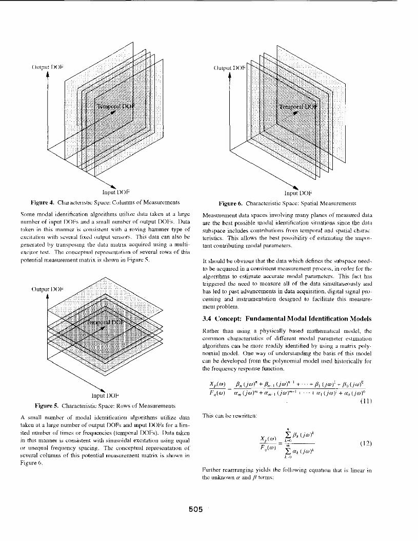
As the sophistication of data a~:quisitinn equipment and modal parameter estimation algorithms evolved. later techniques fit the

data in a plane of the characteristic space. For example. this corre­sponds to the data taken at a number of response points hut from a single excitation point or reference. This representation of a col­umn of measurements is shuwn as one of the planes of information

in Figure 4. Fur this situation. which represents a single input (ref­erence), it is not possible to compute repeated roots ami it is diffi­cult to separate closely coupled modes due to the lack of spatial data. Many modal identification algorithms utilize data taken at a large number nf output DOFs due to excitation at a small number uf tnput DOFs. Data taken in thi:-. manner is consistent with a multi-exCitor type of test. The conceptual representation of several columns nf this potential measurement matrix is shown in Figure 4.

504

Output DOF

Input DOF

Figure 4. Characteristic Space: Columns of Mea<>urements

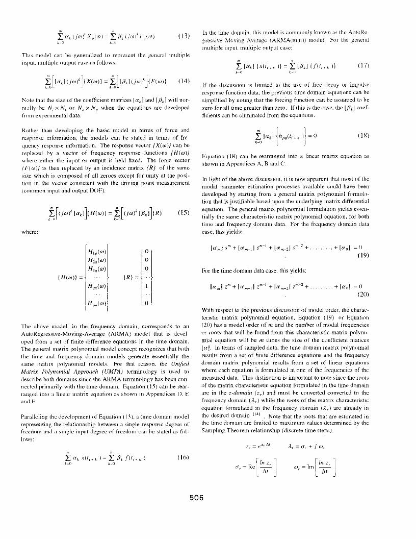
Some modal identification algorithms utilize data taken at a large number of input f)OFs and a small number of output DOFs. Data taken in this manner is consistent with a roving hammer type of excitation with several fixed output sensors. This data can also he generated by transposing the data matrix acquired using a multi­excitor test. The conceptual representation of several rows of this potential measurement matrix is shown in Figure~-

Output DOF

Input

Figure 5. Characteristic Space: Rows of Measurements

A small number of modal identification algorithms utilize data taken at a large number of output DOFs and input DOFs for a lim­ited number of times or frequencies {temporal DOFs). Data taken in this manner is consistent with sinusoidal excitation using equal or unequal frequency spacing. The conceptual representation nf several columns of this potential measurement matrix is shown in Figure 6.

505

Output DOF

DOF

Figure 6. Characteristic Space: Spatial Measurement<>

Measurement data spaces involving many planes of mea'iured data are the best possible modal identification situations since the data subspace includes contributions frnm temporal and ~patial charac­teristics. This allows the best possibility of estimating the impor­tant contributing modal parameters.

It should be obvious that the data which defines the subspace need~ to be acquired in a consistent mea<;urement process, in order fur tht: algorithms to estimate accurate modal parameters. This fact ha.<,; triggered the need to measure all of the data simultaneously and has. led to past advancemenL'i in data acquisition, dig1tal signal pro­cessing and instrumentation designed to facilitate this measure­ment problem.

3.4 Concept: Fundamental Modal Identification Models

Rather than using a physically based mathematical model, the common characteristics of different modal parameter estimation algorithms can be more readily identified hy using a matrix poly­

nomial model. One way of understanding the ba<>is of this model can he developed from the polynomial model used historically fnr the frequency response function.

P" (jw)" + P." 1 (jw)"- 1 + · · · + p, (jw) 1 +Po (jw)0

am (jw)m +am-I (jw)m 1 + · · · + al (jw): + u 0 (jw)0

This can be rewritten:

m

L fXJ.: (jw)k J.:~o

(II)

(12)

Further rearrranging yields the following equation that is linear in the unknown a and f3 terms:

± "' (jw)' X,.(rul ~ ± jJ, (jw{ 1-q(oJI (13) k- ,, k--0

Th1s model can be generalized to represent the general multiple

1nput, multiple output C<L"c as follows:

Note that the size of the coefficient matrices [ad and [fid wtll nor­

mally be N; x N; or N" x N, when the equations are developed from experimental data.

Rather than developing the basic model in terms of force and response infommtion, the models can he stated in terms of fre­quency response information. The response vector {X(w)} can be replaced hy a vector of frequem:y response functions { H(w)}

where either the input or output is held fixed. The force vector (F(w)j is then replaced by an incidence matrix {R) of the same

size which is composed of all zeroes except for unity at the posi­tion in the vector consistent with the driving point measurement (common input and output DOF).

where:

H 1q(w)

rol H 2q(w) 0

H3,(w) 0

(H(wl} ~ (R} ~

Hqq(m)

IH,,,IWI ()

The above model, in the frequency domain, corresponds to an AutoRegressive-Moving-Average (ARMA) model that is devel­oped from a set of finite difference equations in the time domain. The general matrix polynomial modd concept recognizes that both the time and frequency domain models generate essentially the same matrix polynomial models. 1-'or that reason. the Unijit'd Matrix flo(vnrmziul Approach (UMPA) terminology is used to

describe both domains since the ARMA tenninnlogy has been con­nected primarily with the time domain. Equation (15) can be rear­ranged into a linear matrix equation a" shown in Appendices D. E and F

Paralleling thi.! development tlf Equation ( I:'), a time domain model repre,.enting the relationaship between a single response degree of freedom and a sin~le input degree of freedom can be stated as fol­lows:

"' " L "' x(l,.' I~ L /3, f(t,.; I (16) k-0

In the time domain, this nndel is commonly known <h the AutoRe­

gressive Moving-Average (ARMA(nLn)) model. For the general multiple input multiple output case:

m 11

L [",j (x(l,,, I}~ L [jJ,J 1/it,,, I} ( 17) k-0 k-11

If the discussion is limited to the use uf free decay or impulse response function data, the previous time domain equations can he simplified by noting that the forcing function can be assumed to he

zero for all time greater than zero. If this is the case. the [/h J coef­ficients can he eliminated from the equations.

(!X)

Equation ( 18) can he rearranged into a linear matrix equation as shown in Appendices A, B and C.

In light of the above discussion, it is now apparent that most of the modal parameter estimation processes avmlable could have been developed by starting from a general matrix polynomial furmula­tion that is justifiable hased upon the underlying matrix differential equation. The general matrix polynomial formulation yields essen­tially the same characteristic matrix polynomial equation, for both time and frequency domain data. For the frequency domam data case, this yields:

· · + [ (,r ol :::::: 0 (19)

For the time domain data case, this yields:

[am]Zm+[am-tlZm-l+lam-21zm-2 + ......... +[ao] ::::::()

(20)

With respect to the previous discussion of model order. the charac­teristic matrix polynomial equation, Equation ( 19) or Equation (20) has a model order of m and the number of moJ.al frequencies or roots that will he found from this characteristic matrix polyno­

mial equation will he m times the size of the coefficient matices [a]. In terms of sampled data, the time domain matrix polynomial results from <l set of finite difference equations and the frequellcy domain matrix polynomial results from a set of linear equations

where each equation is formulated at one of the frequencies of the measured data. This distinction is llntxJrtant to note since the roots of the matrix characteristic equation fonnulated in the tUne J.omain are in the z-domain (Zr) and must he converted converted tn the frequency domain ( A.r) while the roots of the matrix characteristic

equation formulated in the frequency domain (A.r) arc already in

the desired domain 1141 Note that the roots that are estimated in the time domain are limited to maximum values J.etennined by the Sampling Theorem relationship (discrete time steps).

[In z, ]

(fr= Rc ~ [

In z, ] mr:::::: Irn Tt

506

Domain Matrix Pnlynomial Order Cneffictents

Algorithm Time FrelJ Zero Low High Scalar Matrix

Complex Exponential Algorithm (CEAJ . . . Least Squares Complex Exponential (LSCE) . . . Polyreference Time Domain (PTD) . . N,xN,

Ibrahim Time Dnmam (lTD) . . N0

X N,

Multi-Reference Ibrahim Time Domain (MRITD) . . N0 xN" Eigensystem Realization Algorithm (ERA) . . N"xN" Polyreference Frequency Domain (PFD) . . N,xN,

Simultaneous Frequency Domain (SFD) . . N,xN,

Multi-Reference Frequency Domain (MRFD) . . N,xN,)

Rational Fraction Polynomial (RFP) . . . Hnth

Orthogonal Polynomial (OP) . . . Hoth

Complex Mode Indication Function (CMIF) . . N"xN,

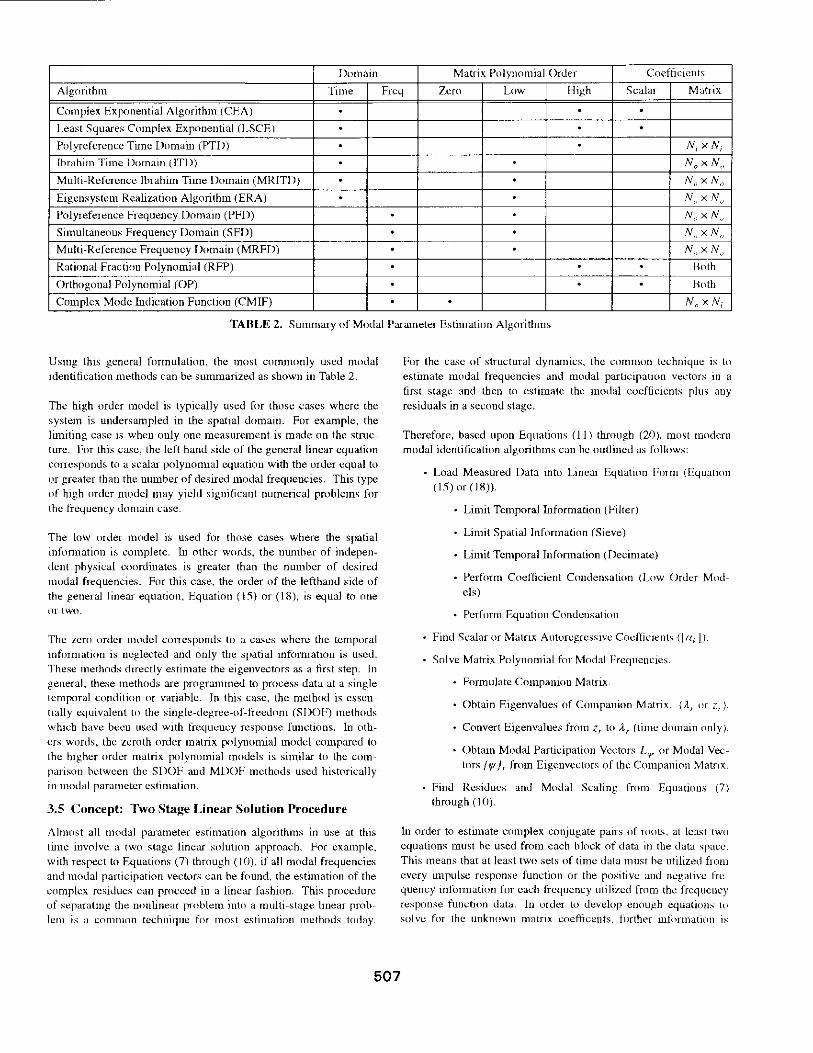
TABLE 2. Summary of Modal Parameter Estimation Algorithms

Usmg this general formulation, the most commonly used modal identification methods can he summarized as shown in Table 2.

The high order model is typically used for those cases where the system is undersampled in the spatial domain. For example, the limiting ca<>e ts when only one measurement is made on the struc­ture. for this case, the left hand side of the general linear equation corresponds to a scalar polynomial equation with the order equal to or greater than the number of desired modal frequencies. This type of high order model may yield significant numerical problems for the frequency domain case.

The low order model is used for those cases where the spatial infunnation is complete. In other words, the number of indepen­dent physical coordinates is greater than the number of desired modal frequencies. For this ca<>e. the order of the lefthand side of the general linear equation, Equation (I)) or (18), is equal to one nr two.

The zero order model corresponds to a cases where the temporal information is neglected and only the spatial infonnation is used. These methods directly estimate the eigenvectors a<> a first step. In general. these methods are progranuned to process data at a single tem[XJral condition or variable. In this case, the method is essen­tmlly equivalent to the single-degree-of-freedom (SDOP) methods which have been used with frequency response functions. In oth­ers words, the zeroth order matrix polynomial model compared to the higher order matrix [XJlynomial models is similar to the com­parison between the SDOF and MDOF methods used historically in modal parameter estimation.

3.5 Concept: Two Stage Linear Solution Procedure

Almost all modal parameter estimation algorithms in use at this time involve a two stage linear solution approach. For example, with respect to Equations (7) through (10), if all modal freLJUencies and modal participation vectors can he found, the estimation of the complex residues can proceed in a linear fashion. This procedure of separating the nonlinear problem into a multi-stage linear prob­lem is a common technique for most estimation methods today.

507

For the case of structural dynamics, the common technique is to estimate modal frequencies and modal participation vectors in a first stage and then to estimate the modal coefficient.<> plus any residuals in a second stage.

Therefore, based upon Equations (11) through (211), most modem modal identification algorithms can he outlined as follows:

Load Measured Data into Linear Equation Form (Equation (15) or (18)).

Limit Temporal Information (Filter)

Limit Spatial Information (Sieve)

Limit Temporal Information (Decimate)

Perform Coefficient Condensation (Low Order Mnd­cls)

Perform Equation Condensation

Find Scalar or Matrix Autoregressive Coefficients (] ak J ).

Solve Matrix Polynomial for Modal Frequencies.

Formulate Companion Matrix.

Obtain Eigenvalues of Companion Matrix. (it,. or Zr)·

Convert Eigenvalues from Zr to itr (time domain only).

Obtain Modal Participation Vectors 1-qr or Modal Vec­tors { ljl j r from Eigenvectors of the Companion Matrix.

Find Residues and Modal Scaling from Eljuations (7) through (I 0).

In order to estimate complex conjugate pairs of rooL,, at least two equations must be used from each block of data in the data space. This means that at least two sets of time data must be utilized from every impulse response function or the positive and negative fre­quency infonnation for each frequency utilized from the frequency response function data. In order to develop enough equations tu solve for the unknown matrix coefficents, further infnrmatitl\1 is

l:lkcn f[llfll the same block of data nr from uthcr blocks !l[ data in 1he data space until the number of equations equals (If exceeds the number of unknnwns (cocflicients). The exact form and require­ments for Equation (IS) or (lR) for many of the com_m(,nly used modal identification algorithms is given in Appendices A through r

Once the matrix cneHit..:ients ((a J) have hecn found, the modal fre­quencies (A.r or Zr) can be found using a number of numerical tech­mqucs. V..'hile m certain numerical s1tU<Hions. other numerical approaches may he more robust_ a companion matrix approach

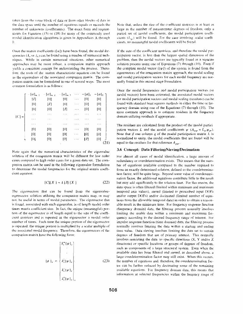
y1elds a consistent concept fot Llt1de!'standing the process. Thcre­fnre. the roots of the matrix characteristic equation can he found as the eigenvalues of the associated t:ompanion matrix. The com­panion matrix can be formulated in one of several ways. The most common formulation is as follows:

-[a],_! -[u],,_::: -[a],_, -[a[, -[ rt[o

l [/] [OJ I 01 I OJ [0]

[OJ [/] [OJ [OJ [0]

I o I [0] [/] [0] [0]

[C[~

[0] [0] [0] [0] Ill]

[0] [0] [0] [0] [OJ

[01 [OJ [0] [/] [0] (21)

Note again !hal the numcri(.;aJ characteristics of the eigenvalue solution of the companion matrix will he different for low order c<~ses compared to high order ca.o;;es for a given data set. The com­panion matrix ~;an he used in the following eigenvalue formulation to determine the modal frequencies for the original matrix cocm­CJcnl equatiOn:

[CJIX l ~ .l[/] {X I (22)

The ei~envcctors that can be found from the cigenvaluc­CI~envcctor solution utilizing the companion matrix may. or may not. he useful in terms uf modal parameters. The cigcnvectlll' that

is found. associated with each eigenvalue. is of length model order times matrix coefficient size. In fact, the unique (meaningful) por­tion of the eigenvector is of length equal tn the size of the coeffi­Cient matrices and is repeated in the eigenvector a model order numher of times. Each time the unique portion of the eigenvector is repeatet.l, the unique portion is multiplied by a scalar multiple uf the associated modal frequency. Therefore, the eigenvectors of the companion matrix have the following form:

!23)

Nutc that. unless the size of the coefficient matrice" is at least as

large as the number of mea~urcment degrees of freedom. only a p;rrtial set of modal coefficienl". the modal participation cncffi­ctents (Lqr) will be found. Fnr the case involving scalar cuefti­cients, no meaningful modal codticients will he found.

If the s1ze uf the coeffit:ient matricl.!s, and therefore the modal pm·­

ticipatmn vector. is less than the largest spatial dimension of the prohlem, then the modal vectors are typically found in a separate solution process using une of Equations (7) through (I 0). Even if

the complete modal vector ({1/f}) of the system is found frnm the eigenvectors of the companion matrix approach, the modal scaling and modal participation vectors for eat:h modal frequency arc nor­

mally found in this second stage formulation.

Once the modaJ frequencies and moJaJ participation vectors (DI

modal vectors) have been estimated, the associated modal vectors (or modal participation vectors and modal scaling (residues) can be found with standard least square.<. mcthmls in either the time or fre­

quency domain using one of the Equations (7) through (10). The most common approach is to estimate residues in the frequency domain utilizing residuals if appropriate.

The residues are calculated from the product of the modal partici­

pation vectors L and the mm1al coefficients If/ (ApQr = L 9,rp,,). Note that if one column q of the modal participation matrix L is normalized to unity, the modal coefficients that arc found will be equal to the residues for that reference Apqr·

3.6 Concept: Data Filtering/Sieving/Decimation

For almost all cases of modal identification, a large amount uf redundancy or overdetenninatinn exists. This means that the num­

ber of equations available compared to the number required tu

form an exactly determined solution. defined as the nvcrdetennina­tion factor, will be quite large. Beyond some value of nven.letenni­nation factor, the additional equations contribute little to the result but may add significantly to the solution time. For this rea~rm, the

data space is often filtered (limited within minimum and maximum temporal axis vaJucs), sieved (lim1ted to prescribed input DOFs and/or output DOFs) and/nr decimated (limited number of equa­tions frotn the allowahle tempnral data) in order tn obtain a reason­

able result in the minimum time. For frequency response functitHJ (frequency domain) data, the filtering process nonnally involves limiting the usable data within a minimum and maximum fre­quency at..:corLiing tn the desired frequency range nf interest. l-ior impulse response function {time domain) data, the filtering process normally involves limiting the data within a starting and ending time value. Data sieving involves limiting the data set to t:ertain degrees of freedom that are of primary interest. This nonnally involves restricting the data to spet:ific directions (X, Y and/or Z directions) or specific locations or groups of degrees of frt::ed(Jm. such as components of a large structural system. Even when the available data has been filtered and sieved, as dc,<;<.:ribed ahove, a large ovcrdeternnination factor may still exist. When this occurs, the number of cquatiuns and. therefore, the nverdetermination fac­tor can he further reduced by del:imating some of the remaining available equations. For frequency domain data. this means that information at selected frequencies within the freqent.:y range of

508

mterest can he eliminated. For time domain data, thn., means that information from different portions of the remaming available time range (overlaps, numher of overlaps, time shift between overlaps) can he eliminated.

3.7 Concept: Coefficient Condensation

For the low order modal identilication algorithms, lht.: number of physical coordinates (typically N,,) i>. often much larger than the number of desired modal frequencies (2N). For this situation. the

numerical solution procedure is constrained to solve for N,, or 2N" modal frequencies. This can be very time consuming and is unnec­essary. The number of physical coordinates (N") can he reduced to a more n:asonahle size (Nr"" N,, or Np"'" 2N") hy using a decom­position transformation from phys1cal coordinates (N,) to the approximate number of effective modal frequencies (Nr). Cur­rently, singular value decompositions (SVD) or eigenvalue decom­positions (ED) arc used to preserve the principal modal mfmma­tion prior to formulating the linear equation solution for unknown

matrix coefficients 17 ·17] In most cases, even when the spatial information must be condt.:!nscd, it is necessary to use a model urder greater than two to compensate for distortion errors or noise in the data and to compensate for the ca.se where the location of the

transducers is not sufficient to totally define the structure.

3.!1 Concept: Equation Condensation

Several important concepts should be delineated in the area of

equation condensation methods. Equation condensation methods arc used to reduce the number of equations ba.sed upon measured data to more closely match the number of unknowns in the modal parameter estimation algorithms. There are a large number of con­

densation algorithms available. Hased upon the modal parameter estJJnation algorithms in use today, the three types of algorithms most often used are:

Least Squares: Least squares (LS), weighted least squares

(WLS), total least squares (TLS) or double least squares (DLS) is used to minirnia: the squared error between the measured data and the estimation model. Historically, this is one of the most popular procedures for finding a pseudo­

inverse solution to an over specified system. The main advantage of this method is computational speed and ease of implementation while the major disadvantage is numerical prects1on

Transformations: There arc a large number nf transfnnna­tion that can he used to reduce the data. In the transfonna­tion methods, the measured data is reduced by appmximat­mg the data hy the superposition of a set of significant vec­tors. The number of significant vectors is equal to the

amount of mdependent mca'iurcd data. This set of vectors is used to approximate the measured data and used as input tn the parameter estimation procedures.

Singular Value Dccompositwn: Singular Value Decomposition (SVD) i~ an example of one of thl' 11111rc p11pular transformati11n methods. The maJor advantage of these methods is numerical precis inn ;md the disadvantage is etnnputatinnal speed and memory req u 1remcn ts

Coherent Averaging: Cohercnl averaging is an1Jther popular method for reducing the data. In the coherent averaging method, the data is weighted by performing a dot product between the data and a weighting vector (spahal filkr). Information in the data which is not coherent With the weighting vectors is averaged nut of the data. The method IS

often referred to as a spatial or modal filtering procedure. This method has both spt.:!td and precision hut. in nrder to achieve precision. requires a good set of weighting vectors. In general, the optimum weighting vectors are connected with the solution which is unknown. It should he noted that least squares is an example of o non-coherent av\:ragmg pnl­

cess.

The least squares ami the transformation procedure>. tends to weight those modes 11f vibration which are well excited This can be a problem when trying to extract modes which are nut well excited. The solution is to use a weighting function for condensa­

tion which tends to enhance the mode of interest. This can be accomplished in a number of ways:

In the time domain, a spatial filtt.:!r or a cohertnt averaging process can be used to filter the response to enhance a partic­ular mode or set of modes. For example, hy averaging the data from two symmetric exciter locations the symmetric modes of vibration can be enhanced. A second example would he using only the data in a local area of the system Ill

enhance local modes. The third method is usin~ cstunates of the modes shapes as weighting functions to enhance particu­

lar modes.

In the frequency domain, the data can be enhanced in the same manner as the time domain plus the data can he addi­tionally enhanced by we1ghting the data in a frequency band ncar the natural frequency of the mode of interest.

Obviously, the type of equation condensation method that is uti­lized in a modal identification algorithm has a significant influence on the result" of the parameter estimation process.

3.9 Concept: Model Order Determination

Much of the work concerned with modal parameter esti.matitln since 1975 has involved methodology for determining the cnm.:ct model order for the modal parameter model. Technically. mndd

order refers to the highest power in the matrix polynomial e4ua­tion. The number of modal frequencies found will be equal to the model order times the size of the matrix coefficients, nnnnally N" or N,. For a given algorithm, the size of the matrix coefficients is normally fixed; therefore, dctennining the model order is duectly linked to estimating N, the number of modal frequencies that are of interest in the measured data. As has always been the ease. ;111

estimate for the minimum number of modal frequencies can he easily found hy countmg the number of peaks in the frcqu-.:nc}

response function in the frequency hand of analys1s. This 1s a mm­imum estnnate of N since the frequency response function mea­

surement may he at a node of one or more mndes nf the system. repeated roots may exist and/or the frequency resolutHlll uf the measurement may be ton coarse to ohscrvc modes that arc close]} spaced in frequency. for these reasons. an appropn<Jtc e-.;timatc td the urder uf the model is of pmne conc~.:rn and 1s the single most

509

illlf1('1t,mt pnthkm ttl nHtdal par:.uneter estllllil{Htn

tn unkr tu determine a rea...,unahle estimate uf the Jll(ll!t:! urder for

c.~ ~et pf tepte:..entalivc data. a number of tt\.:hnH . .JUC::> have been developed a~ guide~ or aids to the user. Much uf the user mter;ll:­uon involved in modal parameter estimation invnlves the u:-.:c uf 1hc:-.:e ruuls. Most of the techniques that have been developed alltJ\V

the ust:r to t:stablisb a maximum nwdcl ~trder to l1e t:valuatcd \111 many cases, thi~ is .-.:ct by the memnry limits of the computer algn­nthmJ. I lata i.:-; <1cquued hased upon an assumption that the mndcl

urder 1s etJual to this maximum. In a sequential fashion, this data 1s evaluated to dett=rminc if a model order less than the maximum

wdi describe the data sufficiently. This is the point that the user's JUdgement and the use of vanous evaluation aids becomes impor­tatH. SlllllC of the nmunonly used techniques are:

Ern.1r Chart.

Stability Diagram.

~v1ode Indication Functions.

Rank Estimation.

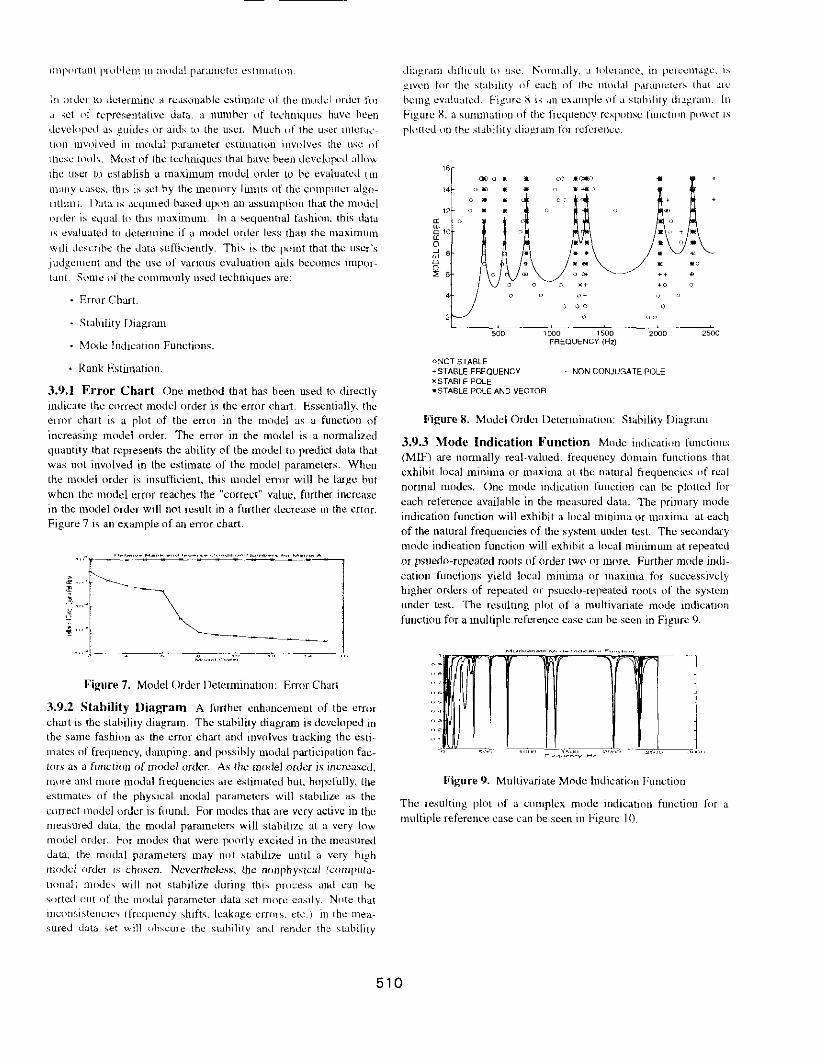
3.9.1 Error Chart One method that has been used to directly indicate the correct model order is the error chart. Essentially, the error chart is a plot of the error in the model as a function of increasmg model order. The error in the model is a normalized quant1ty that represents the ability of the model to predict data that was not involved in the estimate of the model parameters. When the model nrder is insufficient. this model enor will he large but

when the model error reaches the "correct" value, further increase in the model order will not result in a further decrease in the error. Figure 7 is an example of an error chart.

.":

Figure 7. Model Order Determination: Error Chart

3.9.2 Stahility Diagram A further enhancement of the error chart is the stability diagram. The stability diagram is developed in the same fashion as the error chart and involves tracking the esti­mates of frequency, damping. and possibly modal participation fac­tors as a function of model order. As the model order is increased, more and more modal frequencies arc estimated but. hopefully, the estunal~.:s of the physical modal parameters will stabilize as the

correct model order is fuund. For mndes that are very active in the measured data, the modal parameters will stabilize at a very low model order. For modes that were poorly excited in the measured data, the mndal parameters may not .'>tabilize until a very high model order is chosen. Neverthele.<.:s, the nonpby.qca! lcnmruta­

tinnal l mnde" will not stahilize during thi.'"> proc.:ess and can he sorted out nf the modal parameter data set more easily. Note that I!H:on~i~tcnclC'-. (frequency ~hift<•. leakage errors. etc.) in the mea­sured tbta '-Ct will ohscure the >;tahility and render th<:". '">tahility

diagram difflcull tu usc. Nurm,lily. ~ tuleranc~. in percenta~c. 1:.

~1ven for the stability uf each uf the mmlal p<~r:.Ullctcrs that ,uc bcmg evaluated. Figure X 1s ,m example uf a stability diagran1. In

Figure X, a sununati11l1 of the frequency rexpunsc functi111l powcr 1~ pJutted Ull the stability dia~ram for rcfcre!lcC.

" 000 • • 00 •c::.o 14 0~ • • ·~' 0 • • 12 • •

~ w 010 • ~ 0 • • • ~ 6 . • w • 0 0

~

~ 6 0 ~ H

0 0 •o 4 0 o•

0 00 0

500 1000 1500 2000

oNOT STABLE +STABLE FREQUENCY XSTABLE POLE •STABLE POLE AND VECTOR

FREQUENCY (Hz)

NON-CONJUGATE POLE

• 0 •

•c •

2500

Figure 8. Model Order Determination: Stability Diagram

3.9.3 Mode Indication Function Mndc indication functions (MIF) are nonnally real-valued. frequency dnmain functions that exhibit local minima or maxima at the natural frequencies of real normal modes. One mode indication function can be plotted fnr

each reference available in the measured data. The primary mode indication function will exhibit a local minima or maxima at each of the natural frequencies of the system under test. The secondary mode indication function will exhibit a lol:a! minimum at repeated

or psuedo-rcpeated mots of order two nr more. Further mode indi­cation functions yield local minima or maxima for successively higher orders of repeated or psucdo-repeated roots of the system under test. The resulting plot of a multivariate mode indication function for a multiple reference case can be seen in Figure 9.

I'

'',.,

Figure 9_ Multivariate Mode Indication Function

The resulting plot of a complex mode indication function for a multiple reference case can he seen in Figure 10.

510

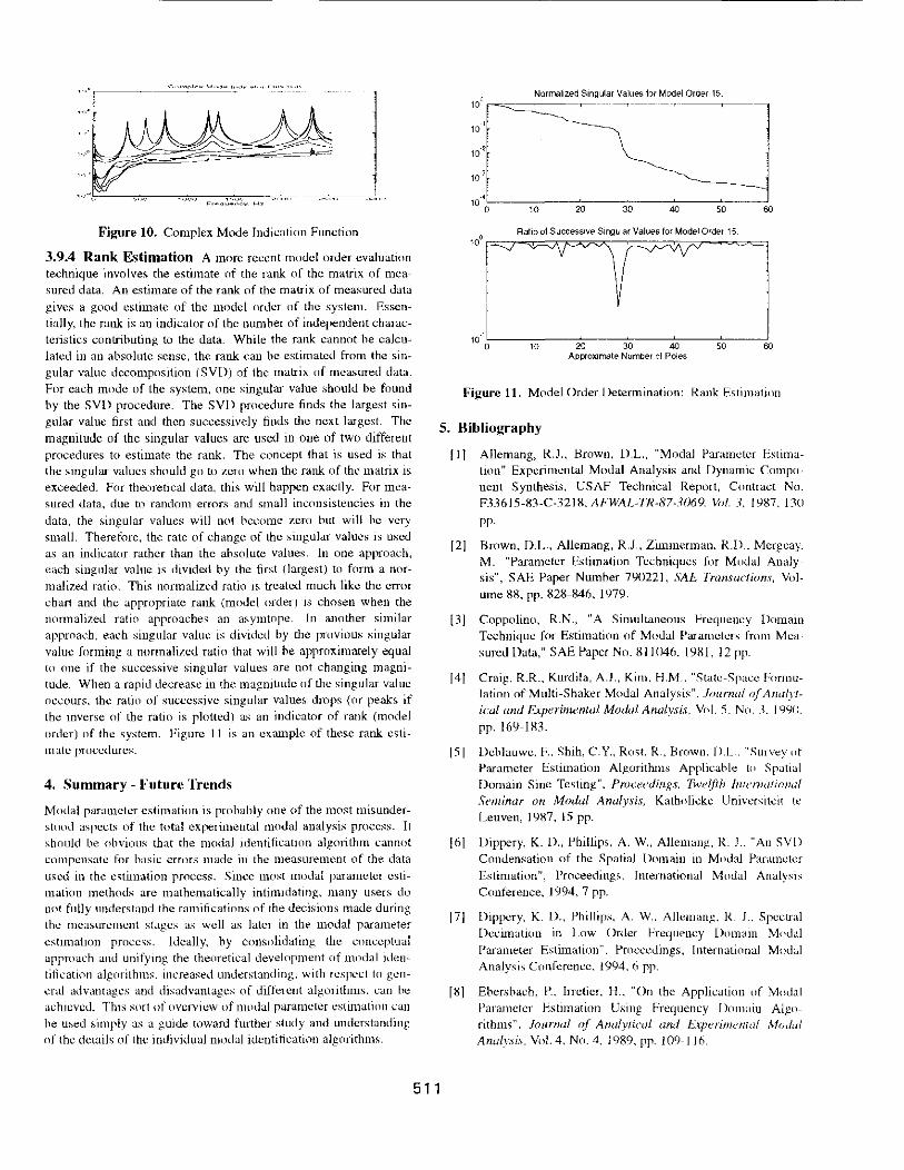
Figure 10. Complex Mode Indication Function

3.9.4 Rank E~timation A more recent model order evaluation technique involves the estimate of the rank of the matrix of nH.:a~ surcd data. An estimate of the rank of the matrix of measured data gives a good estimate of the model nrder of the system. Essen­tially, the rank is an indicator of the number of independent charac­teristics contributing to the data. While the rank cannot he calcu­lated in an absolute sense, the rank can be estimated from the sin­gular value decomposition ( SVD) of the matrix of measured data. For each mode of the system, one singular value should be found by the SVD procedure. The SVD procedure finds the largest sin­gular value first and then successively finds the next largest. The magnitude of the singular values are used in one of two different procedures to estimate the rank. The concept that is used is that the smgular values should go to zero when the rank of the matrix is exceeded. For theoretical data. this will happen exactly. For mea­sured data, due to random errors and small inconsistencies in the data, the singular values will not become zero hut will he very small. Therefore, the rate of change of the singular values is used as an mdicator rather than the absolute values. In one approach, each singular value is divided by the first (largest) to form a nor­malized ratio. This normalized ratio 1s treated much like the error chart and the appropriate rank (model order) is chosen when the normalized ratio approaches an m;ymtope. In another similar approach, each singular value is divided by the provious singular value forming a normalized ratio that will he approximately equal to one if the successive singular values are not changing magni­tude. When a rapid decrea'ie in the magnitude of the singular value occours. the ratio of successive singular values drops (or peaks if tht! inverse of the ratio is plotted) a..;.; an indicator of rank (model order) of the system. Figure 11 is an example of these rank esti­mate procedures.

4. Summary - Future Trends

Modal parameter estimation is probably one of the most misunder­stood aspects of the total experimental modal analysis process. It should be obvious that the modal identification algn1ithm cannot compensate for basic errors made in the measurement of the data used in the estimation process. Since most modal parameter esti­mation methods are mathematically intimidating, many users do not fully understand the ramifications of the decisions made during the measurement stages a." well as later in the modal parameter cstunallon process. Ideally, hy CmiS(Jlidatirig the Conceptual approach and unifying the theoretical development of modal iden­tillcatinn algorithms. increased understanding. with respect to gen­eral advantages and disadvantages of different algorithms, can be achieved. This sPrt of overview of nwdal parameter estimation can he uo,ed simply as a guide toward further study and understanding of the details nf the individual modal identification algorithms.

10'

10·~~-----,~oc-----~,o~----~3~0------40~-----o,o~----~60

0 Ratio of SuccessiVe Singular Values for Model Order 15

10

[~~ =~1

, I • 0 10 ~ ~ ~ ~ 00

Approximate Numoer of Poles

Figure 11. Model Order Determination: Rank Estimation

5. Biblio1,..-aphy

[1J Allemang, R.J., Brown, D.L., "Modal Parameter Estima­tion" Experimental Modal Analysis and Dynamic Compo­nent Synthesis, USAF Technical Report, Contract No. F33615-83-C-3218. AFWAL-TR-87-3069. Vol. 3. ln7. 130

pp.

[2J Brown, D.L., Allemang, R.J., Zimmerman, R.D .. Mcrgeay. M. "Parameter Estimation Techniques for Modal Analy­sis", SAE Paper Number 790221, SAE Tranwctions, Vol­ume 88. pp. 828-846, 1979.

[3 J Coppolino, R.N., "A Simultaneous hequency Domain Technique for Estimation of Modal Parameters from Mea­sured Data," SAE Paper No. 811046. 1981, 12 pp.

[41 Craig. R.R., Kurdi!a, A.J .. Kim. H.M .. "State-Space Formu­lation of Multi-Shaker Modal Analysis", Journal (if Analyt­ical and Experimental Modal Analysis. Vol.). Nn. ~. I 991l. pp. 169-183.

511

[5] Dcblauwe, F.. Shih, C.Y., Rost. R., Brown. D.L.. "'Survey of Parameter Estimation Algorithms Applicable tP Spatta! Domain Sine Testing". Pmn:edinxs. Twelfth /nremational Seminar on Modal Analysis, Katholieke Univcrsitcit te Leuven, 1987, 15 pp.

[6[ Dippery, K. D., Phillips, A. W., Allemang, R. 1.. '"An SVD Condensation of the Spatial Domain in M11dal Parameter Estimation". Proceedingf.., International Mt1dal Analysis Conference, I 994, 7 pp.

[71 Dippery, K. D .. Phillips. A. W., Allemang. R. 1.. Spccu·al Decimation in Low Order frequency Domain Modal Parameter Estimation·· Proceedings. International Modal Analysis Conference, 1994, 11 pp.

pq Ebersbach, P .. Irretier, H .. "On the Application uf Modal Parameter Estimation Using Frequency Domain Algo­rithms", Journal of Analyiical and I!J..paimema/ Modal Analysis. Vol. 4, No.4, 19R9, pp. 109-116.

flJ[ Fukuzuno. K.. "lnvc~tt~.Jtiun lll ~1ullipk-Rdcrcnce

lhr~lhim Tune Domain Mudal Parameter b'~timatam Tech­

nique." M. S. Thesis. Depl. llf Mt::ch.J.nica\ and lnduSirlal Engmeering. University of C'uKumatl. I YXO. 22( l PI'

[ \0[ Hollkamp . .! . .!.. Hatill. S.M .. "A Recur..;tve -\l~urithm fur

J)iscrete Time \)omain Paramekr ldcntitic,Ltlllll" .-\IAA

Paper No. AIAA-90-1221, I YYtl, I 0 pp.

{II] Hou. Z.Q .. Cheng. Y.D .. Tong. Z.F .. Sun. Y.M .. lu. N.Y., "Modal Parameter ldcntili~;atl~1ll frutn Multi-Pumt Mea­

sured Data." Procndings. /!llt'rrwtional Modal Anulvsis Con_fat'nct'. Society nf Experimental Mechanics [SEMl.

198S.

[121 Ibrahim. S. R .. Mikulcik. E. C. "A Method for the llircct fdentitication of Vibration Parameters frnm the Free Response." S'Jwck and Vihration Rullt'tin, Vnl. 47. Part 4

1 Y77. rr- 183-I Y8.

[13] .luang, Jer-Nan. Pappa. RichardS .. "An Eigensystem Real­

ization Algorithm for Modal Parameter Identification and Mndd Reduction". AIM Journal of (1uidanct', Control. and !Jynamics, Vol. 8, No.4, 1985, pp. 620-627.

[ !4J Jury, E. I.. Theory and Application of the z-Transform Method". John Wiley and Sons, Inc. 1964,330 pp.

[ 15] Kabe, A.M .. "Mode Shape Identification and Orthogonal­

ization" USAF Space Division Report SD-TR-88-93,

I9XX. 2'> rr-

[ 16] Lee, G.M .. Trethewey, M.W., "Modal Parameter ()uality

Assessment from Time Domain Data", Journal of Analyti­cal and Experitnt'ntal Modal Analysis, Vol. 3. No.4, 198R,

rr- 129-m,_

[ I7] Lcmbregt<>, F., "Frequency Domain Identification Tech­

niques for Experimental Multiple Input Modal Analysis",

Ph. D. Dissertation, Katholiekc Universiteit Leuven, Leu· ven, Belgiwn. 1988.

[ 18[ Lemhrcgts, F .. Lcuridan . .1 .• Zhang. L., Kanda. H., "Multi­

ple Input Modal Analysis of Frequency Response Func­

tions bascO un Direct Parameter Identification." Proct't'd­ings. International Modal Analysis Conference, Society of Ex.perunental Mechanics (SEM). IY86.

[ IY] Lembregl<>, F., Leuridan. J.L.. Van Hrussel. H .. "Frequency

Domain Direct Parameter Identification for Modal Analy­Sis· State Space Fnnnulatwn". Mahanical .\vstt'ms and Signal Processing. Vol. 4. No. I. 1989. pp. 65-76.

(20] Leonard. F.. ''ZMODAL: A New Modal Identification

Techmque". Journal of Analytiealand Expaimental Modal Analysis. Vol. .'. No. 2. 1988. pp. 69-76.

[21] I .curidan . .1. "Some Direct Parameter Model IdentificatHlll

Methods Applicable fnr Multiple Input Modal Analys1s,"

Doctoral Dtssercatwn. Umversrty of Cincinnati. 1984. 1R4

rr

[22] !.ink. M Vn\Lm. A. "IdentitlcatJnn ()f Structural System

Parameters from Dynamic Rcspnnsc Data." /.cJtschnft F-u1 FlugwJ:>.,.,enschaften. Vol. 2_ Nu. ~ I 97X. pp. I t-:"i-! 7-1-

512

[2 q I ungm.tn, Ri ... ·h~trd W. Ju~l!l~ .. l.-1 Nan, "R,_·.._·tiiSJ\'t' hnm llf

the Eigensy.-.;tem Kt~,llizatilltl Algorithm fm Sy~tcm ldentili­

c .. tti()n" .1./A.A . .luumai ~~1 (;uidwu·t>_ Control. u11d 0\'1111111· in·. Vul. 12, NP. "i. 19X9, pp. O---l7-0'i2

[24] Natke, H.Cl .. "Upd<lling C'llmputational Mllliels in the r--n: qucnn \)umaltl Hased un Me,tsured !lata· A Survey".

l'rol>ahiltstic F'nginet'ring ,\tlecfwnid Yld. ~. Nu. \. l lJXX,

pp. 2X- ~."i

[25} Richardson, M., Fmmenti, lU ... "~'aramdcr btunat1un

frum Frequency RcspllllSC Measurements Using Ratiunal

Fwction Polynmmals." Pmceedings, lnlt'malionai iHodal Analysis Confen:-nce. Society nf C:xpcruncntJl Mel.'hanJc . ..;

(SEM). IYn pp. ln7-IX2.

[26] Shih. C.Y.. "Inve~tigation uf Numerical Conditinnin~ in the

frequency l)JHnain MlHlal Parameter E:--.timutillll Mcth1Kls". Doctoral Dissertation. University of Cincinnati. JLJ89. 127

rr-{27] Van der Auweraer. H., Leuridan. .1.. "Multiple Input

Orthugonal Polynomial Parameter Estimation". Mechllniml Systems and Signal Proct>Ssing, Vol. 1. No.3. 1987. pp.

259-272.

{28] Van dcr Auweraer, H .. Snoeys, R., Leuridan. J.M .. "A Global Frequency Domain Modal Parameter Estimation

Technique for Mini-computers," ASME Journal n.f Vilmi· lion. Acoustio, Strl!ss, and Rl'liahility in [)esign, 19XO. 10 pp.

[29] Void, H., "Orthogonal Polynomials in the Polyrcferencc Method," Proceedings. Pmcet'dings, lntt'rnatiotwl Seminllr on Modal Analysis, Katholicke University of Leuvcn. Hcl­gium, 1986.

[30] Vol d. H., Kundrat, J., Rocklin, T.. Russell. R .. "A Multi­Input Modal Estimatitlll Algt1rithm f(Jf Mini-Ctllnputcrs."

SAE Transactions, Vol. 91, No. 1, January I YX2, pp. 815-821.

{31] Vold, H., Rocklin, T "The Numerical Implementation of a

Multi-Input Modal Estimatinn Algorithm for Mini­

Computers," Pron't'Jings, Jnrarwtional Modal AnalyJi.\· Confaence. Society of Experimental Mechanics (SEM}.

rr- 542-548, !982.

[321 Yam, Y., Bayard, lJ.S., Hadaegh, FY., Mettler. E., Milman, M.H., Scheid, k.E., "Autonomous Frequency Domain Iden­

tification: Theory and Experiment", NA.\'A/1 /'L /'ubiication 89-8. 1989, 204 pp.

[33] Zhang, L.. Kanda, H .. Hrown. D.L. Allemang, R.J. "A Pnlyreference Frequency Domain Method for Modal Parameter Identification." ASME Paper Nn. X:"i-DET-106

I98'i. s rr-

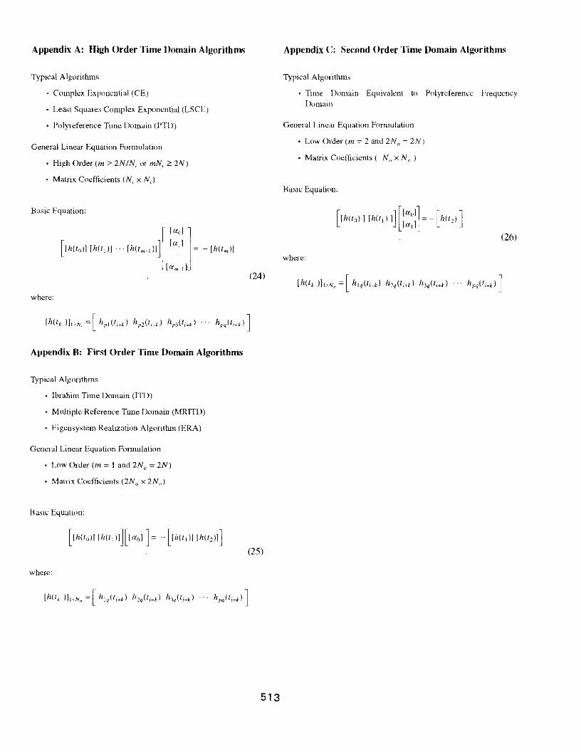
Appendix A: High Order Time Domain Algorithm'

Typtcal Algorithms

Complex Exp(mential (CE}

Lea"t Squares Complex Exponential {LSCJ-::)

Polyrcference Time Domain (PTD)

General Linear Equation Formulation

High Order (m ~ 2N!N, or mN, ~ 2N)

Matrix Coefficients (N, x N,)

Basic Equation:

[

I rr,l l [ J

lrrtl fh(t,)]]h(ll )] · · · fh(lm-1 )] . . =

[0:',.,_1 J

where:

- fh(lmJJ

Appendix 8: First Order Time Domain Algorithms

Typical Algorithms

Ibrahim Time Domain (TTl))

Multiple Reference Time Domain (MRITD)

Eigensystem Realization Algorithm (ERA)

General Linear Equation Formulation

Low Order (m::: I and 2N0 :::: 2N)

Matrix Cocfllcients (2N, x 2N,)

Hasi~: Equation:

where:

(24)

(25)

513

Appendix C: Second Order Time Domain Al):orithms

Typical Algorithms

Time Domain Equivalent to Polyreferencc Frequency Dum am

General I jncar Equation Fonnulation

Low Order (m::::: 2 and 2N0 ::::: 2N}

Matrix Cncflicients ( N, x N" )

Hasil: Equation;

where:

(26)

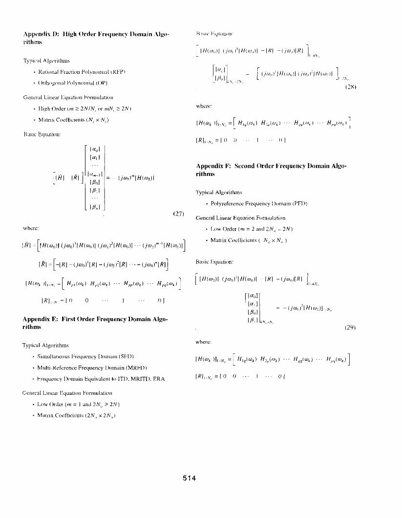
Appendix D: High Order Frettuenfy Domain Algo­rithms

Typtcal Alg!1rlthm~

Ralinna! Fractit1n Pnlynnmial (RFPl

OrtbtJgonal Pulynomial (OP)

General Linear Jc:quatiun Fonnulatnm

High Order(m ~ 2NIN, ur mN, ~ 2N)

Matnx CpeffiCietHs (N, x N,)

K.tsJc b.jUJtion:

IHJ

where:

IRJ J [rt,._ 1 J

I Pol

I p, J

127)

[H] =[[H(w0 )j (jw0 )1[H(w0 )] (jw,,)'[H(w0 )] · ·· (jw11 )"'

1[H(w0 )]]

I R[ = [ -[R] - l)wo)1 I R] - (JwoJ'IR] · ·- Uwol"IRI]

0 o I

Appendix E: First Order Fre<Juency l>omain Algo­rithms

Typical Algonthm~

Simultaneous Frequency Domain (SFD)

Multi-Reference Frequency Domain (MRFD)

Frequency Domain Equivalent to lTD, MRITD, ERA

General Linear Equation Formulation

Low Order (m:::: I and 2N., ~ 2N)

Matrix Coefficient~ (2N., x 2N,)

Ha:-;1,_· Equ:llHlll

where:

llj

Appendix F: Second Order Frequency Domain Algo­rithms

Typical Algorithms

• Pnlyreference Frequency Domam (PFD)

General Linear Equation Fllfll1Uiatinn

Luw Order (m::: 2 and 2N" = 2N)

Matrix Coefficients ( N, x N, )

Basic Equation:

(24)

where:

OJ

514