Model-based approach to envelope and positive …saito/data/phase/kumaresan-rao.pdfModel-based approach to envelope and positive instantaneous frequency estimation of signals with

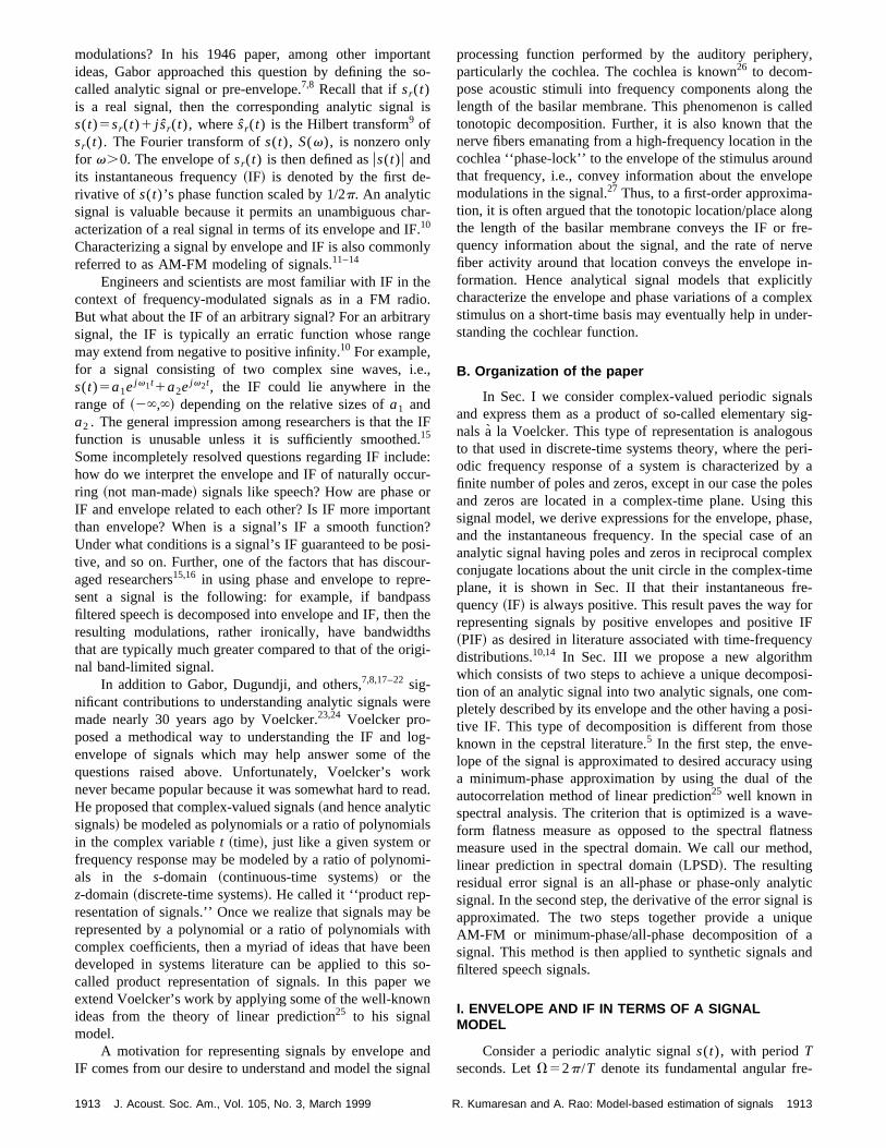
Model-based approach to envelope and positive instantaneousfrequency estimation of signals with speech applications

Ramdas Kumaresan and Ashwin RaoDepartment of Electrical Engineering, University of Rhode Island, Kingston, Rhode Island 02881

~Received 15 May 1997; accepted for publication 6 November 1998!

An analytic signals(t) is modeled over aT second duration by a pole-zero model by consideringits periodic extensions. This type of representation is analogous to that used in discrete-time systemstheory, where the periodic frequency response of a system is characterized by a finite number ofpoles and zeros in thez-plane. Except, in this case, the poles and zeros are located in thecomplex-time plane. Using this signal model, expressions are derived for the envelope, phase, andthe instantaneous frequency of the signals(t). In the special case of an analytic signal having polesand zeros in reciprocal complex conjugate locations about the unit circle in the complex-time plane,it is shown that their instantaneous frequency~IF! is always positive. This result paves the way forrepresenting signals by positive envelopes and positive IF~PIF!. An algorithm is proposed fordecomposing an analytic signal into two analytic signals, one completely characterized by itsenvelope and the other having a positive IF. This algorithm is new and does not have a counterpartin the cepstral literature. It consists of two steps. In the first step, the envelope of the signal isapproximated to desired accuracy using a minimum-phase approximation by using the dual of theautocorrelation method of linear prediction, well known in spectral analysis. The criterion that isoptimized is a waveform flatness measure as opposed to the spectral flatness measure used inspectral analysis. This method is called linear prediction in spectral domain~LPSD!. The resultingresidual error signal is an all-phase or phase-only analytic signal. In the second step, the derivativeof the error signal, which is the PIF, is computed. The two steps together provide a unique AM-FMor minimum-phase/all-phase decomposition of a signal. This method is then applied to syntheticsignals and filtered speech signals. ©1999 Acoustical Society of America.@S0001-4966~99!01003-6#

PACS numbers: 43.72.Ar@JLH#

eondazilvtruceriolyr

onlsavalprioncs2

rtaelaob

iseg-

ononfew

areion/ter-tele-hort-

ofatedatathis

ntinghich

sig-ndal’souse, islope

INTRODUCTION

Many natural and man-made signals of interest are timvarying or nonstationary in nature, i.e., their frequency ctent or spectrum changes with time. Examples incluspeech signals, animal calls, biological/biomedical signsuch as cardiac rhythms, etc. Techniques for characterisuch signals are of great importance in applications invoing such signals. A collection of short-time Fourier specknown as spectrogram is a common tool for analyzing stime-varying signals. Unfortunately, the spectrogram sufffrom the need to compromise time and frequency resoluti.e., a large time window is required to resolve closespaced frequencies. To overcome this problem, a numbeso-called time-frequency distributions or representatihave been developed.1,2 The time-frequency analysis tooare very useful in visualizing the time and frequency behior of simple signals like a chirp. However, when the signare complex, as in the case of speech, it is hard to intertime-frequency representations because of the interactbetween components in the signal. The time-frequeanalysis methods also create a practical problem. They rein enormous 2D data sets. Although sometimes thesedata sets can be viewed by humans to sort out the impofeatures of interest, it is hard to program a machine to rably extract such features. Hence it has been difficult toply these methods to automatic signal classification prlems.

1912 J. Acoust. Soc. Am. 105 (3), March 1999 0001-4966/99/105

--elsng-

ahsn,

ofs

-setnsyultDnti-p--

In the area of speech processing, the above problemcircumvented by directly extracting features from short sments of a speech signal. Such algorithms are basedshort-term spectral analysis in the form of linear predicti~which captures the spectral envelope of a signal with aparameters!,3,4 cepstral analysis,5 and Mel-cepstrum.6 Usingthese procedures, spectral templates or feature vectorscomputed and used in applications like machine recognitverification. However, these methods are vulnerable to inference and channel degradations as encountered inphone speech. Signals are also often analyzed over stime intervals, using specific signal models, such as sumsinusoidal or damped sinusoidal signals or phase-modulsinusoidal signals. If such models are appropriate for the dat hand, then significant advantages can be gained. Inpaper a model-based approach is proposed for represesignals by their envelope and instantaneous frequency wis guaranteed to be positive.

A. Envelope and instantaneous frequency of signals

Many of the above-mentioned methods represent anal by characterizing its power as a function of time afrequency. Are there other alternatives? Clearly, a signphase and envelope carry information about how varicomponents of the signal are related to each other. Hencit possible to characterize a signal by its phase and enve

1912(3)/1912/13/$15.00 © 1999 Acoustical Society of America

ans

l

-

ha.n

heio

arge

e.

e.durotan

osouest

thig

er

logthr

re

lsrm

bitheeswn

ndgn

ry,

thelledhethendpe-ng

fre-rvein-tlyplexer-

alssig-useri-y a

olesthisase,f anlex

mere-or

IFcy

osi-m-osi-e

-ing

the

ve-nessod,

yticl isueand

-

modulations? In his 1946 paper, among other importideas, Gabor approached this question by defining thecalled analytic signal or pre-envelope.7,8 Recall that ifsr(t)is a real signal, then the corresponding analytic signas(t)5sr(t)1 j sr(t), wheresr(t) is the Hilbert transform9 ofsr(t). The Fourier transform ofs(t), S(v), is nonzero onlyfor v.0. The envelope ofsr(t) is then defined asus(t)u andits instantaneous frequency~IF! is denoted by the first derivative of s(t)’s phase function scaled by 1/2p. An analyticsignal is valuable because it permits an unambiguous cacterization of a real signal in terms of its envelope and IF10

Characterizing a signal by envelope and IF is also commoreferred to as AM-FM modeling of signals.11–14

Engineers and scientists are most familiar with IF in tcontext of frequency-modulated signals as in a FM radBut what about the IF of an arbitrary signal? For an arbitrsignal, the IF is typically an erratic function whose ranmay extend from negative to positive infinity.10 For example,for a signal consisting of two complex sine waves, i.s(t)5a1ej v1t1a2ej v2t, the IF could lie anywhere in therange of~2`,`! depending on the relative sizes ofa1 anda2 . The general impression among researchers is that thfunction is unusable unless it is sufficiently smoothed15

Some incompletely resolved questions regarding IF incluhow do we interpret the envelope and IF of naturally occring ~not man-made! signals like speech? How are phaseIF and envelope related to each other? Is IF more importhan envelope? When is a signal’s IF a smooth functioUnder what conditions is a signal’s IF guaranteed to be ptive, and so on. Further, one of the factors that has discaged researchers15,16 in using phase and envelope to reprsent a signal is the following: for example, if bandpafiltered speech is decomposed into envelope and IF, thenresulting modulations, rather ironically, have bandwidthat are typically much greater compared to that of the ornal band-limited signal.

In addition to Gabor, Dugundji, and others,7,8,17–22sig-nificant contributions to understanding analytic signals wmade nearly 30 years ago by Voelcker.23,24 Voelcker pro-posed a methodical way to understanding the IF andenvelope of signals which may help answer some ofquestions raised above. Unfortunately, Voelcker’s wonever became popular because it was somewhat hard toHe proposed that complex-valued signals~and hence analyticsignals! be modeled as polynomials or a ratio of polynomiain the complex variablet ~time!, just like a given system ofrequency response may be modeled by a ratio of polynoals in the s-domain ~continuous-time systems! or thez-domain~discrete-time systems!. He called it ‘‘product rep-resentation of signals.’’ Once we realize that signals mayrepresented by a polynomial or a ratio of polynomials wcomplex coefficients, then a myriad of ideas that have bdeveloped in systems literature can be applied to thiscalled product representation of signals. In this paperextend Voelcker’s work by applying some of the well-knowideas from the theory of linear prediction25 to his signalmodel.

A motivation for representing signals by envelope aIF comes from our desire to understand and model the si

1913 J. Acoust. Soc. Am., Vol. 105, No. 3, March 1999

to-

is

r-

ly

.y

,

IF

e:-rnt?i-r-

-shesi-

e

-ekad.

i-

e

no-e

al

processing function performed by the auditory peripheparticularly the cochlea. The cochlea is known26 to decom-pose acoustic stimuli into frequency components alonglength of the basilar membrane. This phenomenon is catonotopic decomposition. Further, it is also known that tnerve fibers emanating from a high-frequency location incochlea ‘‘phase-lock’’ to the envelope of the stimulus arouthat frequency, i.e., convey information about the envelomodulations in the signal.27 Thus, to a first-order approximation, it is often argued that the tonotopic location/place alothe length of the basilar membrane conveys the IF orquency information about the signal, and the rate of nefiber activity around that location conveys the envelopeformation. Hence analytical signal models that explicicharacterize the envelope and phase variations of a comstimulus on a short-time basis may eventually help in undstanding the cochlear function.

B. Organization of the paper

In Sec. I we consider complex-valued periodic signand express them as a product of so-called elementarynals ala Voelcker. This type of representation is analogoto that used in discrete-time systems theory, where the podic frequency response of a system is characterized bfinite number of poles and zeros, except in our case the pand zeros are located in a complex-time plane. Usingsignal model, we derive expressions for the envelope, phand the instantaneous frequency. In the special case oanalytic signal having poles and zeros in reciprocal compconjugate locations about the unit circle in the complex-tiplane, it is shown in Sec. II that their instantaneous fquency~IF! is always positive. This result paves the way frepresenting signals by positive envelopes and positive~PIF! as desired in literature associated with time-frequendistributions.10,14 In Sec. III we propose a new algorithmwhich consists of two steps to achieve a unique decomption of an analytic signal into two analytic signals, one copletely described by its envelope and the other having a ptive IF. This type of decomposition is different from thosknown in the cepstral literature.5 In the first step, the envelope of the signal is approximated to desired accuracy usa minimum-phase approximation by using the dual ofautocorrelation method of linear prediction25 well known inspectral analysis. The criterion that is optimized is a waform flatness measure as opposed to the spectral flatmeasure used in the spectral domain. We call our methlinear prediction in spectral domain~LPSD!. The resultingresidual error signal is an all-phase or phase-only analsignal. In the second step, the derivative of the error signaapproximated. The two steps together provide a uniqAM-FM or minimum-phase/all-phase decomposition ofsignal. This method is then applied to synthetic signals afiltered speech signals.

I. ENVELOPE AND IF IN TERMS OF A SIGNALMODEL

Consider a periodic analytic signals(t), with periodTseconds. LetV52p/T denote its fundamental angular fre

1913R. Kumaresan and A. Rao: Model-based estimation of signals

y

t

.cl

sn

,

r

nceitivclIelclafedd-d

o

s

nitee

-wne

mx-

.

it

or

al

-

f

he

st

helyfyumxite

ex

quency. Ifs(t) has finite bandwidth, it may be described bthe following model for a sufficiently largeM, over an inter-val of T seconds:

s~ t !5ej v tt(k50

M

akejkVt. ~1!

ej v tt represents a frequency translation. In other words,v t

>0 is the nominal carrier frequency of the signal.ak are thecomplex amplitudes of the sinusoidsejkVt; a0Þ0 and aM

Þ0. By analytic continuation we may regardej Vt as a com-plex variable~a la the complex variableZ!. That is, t, thetime variable, is regarded as complex-valued. Note thaEq. ~1! the M th degree polynomial inej Vt represents thecomplex envelope of the signals(t). We may factor thispolynomial into itsM (5P1Q) factors and rewrites(t) as

~2!

p1 ,p2 ,...,pP , and q1 ,q2 ,...,qQ denote the polynomial’sroots; pi5upi uej u i, qi5uqi uej f i. pi denote roots inside theunit circle in the complex plane,qi are outside the unit circleCurrently we assume that there are no roots on the cirThat is upi u,1 and uqi u.1. Each factor of the form (12pie

j Vt) in the above is called an ‘‘elementary signal.’’23

The pi andqi are referred to as zeros of the signals(t). Theabove expressions, representing a band-limited periodicnal, may be recognized as the counterpart of the frequeresponse of a finite impulse response~FIR! filter in discrete-time systems theory.28 More generally, ifs(t) consists of aninfinite number of spectral [email protected]., its Fourier transformS(v)5(k50

` akd(v2kV)#, then we can represents(t) overT seconds to desired accuracy using a sufficient numbepoles and zeros as follows:

~3!

pi and qi correspond to zeros inside and outside the ucircle, respectively.ui correspond to the signal’s poles. Sinthe spectrum of the signal is assumed to have only posfrequencies, poles are restricted to be inside the unit cirAgain this representation is analogous to causal, stablefilters in discrete-time systems literature. Even more genally, if the spectrum ofs(t) is two-sided then we may modes(t) using poles and zeros inside and outside the unit cirej v tt, the arbitrary frequency translation, is analogous toarbitrary time shift in the impulse response in the case odiscrete-time filter. In summary, we model complex-valuperiodic signals using an all-zero or a pole-zero signal moas in Eqs.~2! and~3!, respectively. This type of signal modeling goes back to the work of Cauchy and Hadamard anrelated to the theory of entire functions.29,30 Voelcker calledthis way of modeling signals as ‘‘product representation


in

e.

ig-cy

of

it

ee.IRr-

e.na

el

is

f

signals.’’ We shall primarily work with the all-zero modelsince they are easier to use.

The factors corresponding to the zeros inside the ucircle, P i 51

P (12piej Vt), constitute the minimum-phas

~MinP! signal. Similarly, the factors corresponding to thzeros outside the circle,P i 51

Q (12qiej Vt), constitute the

maximum-phase~MaxP! signal. These are the direct counterparts of the frequency responses of the well-knominimum-and maximum-phase FIR filters in discrete-timsystems theory;5 just as in systems theory~see Sec. 10.3 inRef. 5! the phase of the MinP signal is the Hilbert transforof its log-envelope. That is, the MinP signal may be epressed in the formea(t)1 j a(t). See Appendix A for detailsa(t) is the Hilbert transform ofa(t). Similarly, since amaximum-phase~MaxP! signal has zeros outside the un

circle, it may be expressed aseb(t)2 j b(t). Thus, envelope orphase alone is sufficient to essentially characterize a MinPa MaxP signal.@Along the same lines, an all-phase~AllP!analytic signal~the analog of an all-pass filter! would be ofthe formej g(t).# Thuss(t) may be expressed as

~4!

where the ‘‘hat’’ stands for Hilbert transform.vc is QV~contributed by the linear phase term from the MaxP sign!plus the arbitrary frequency translation,v t , shown in Eq.~2!. Ac is a0P i 51

Q (2qi). See Appendix A for details. Theexpressions fora(t) andb(t) are derived in Appendix A.

a~ t !5 (k51

`

(i 51

P

2upi uk

kcos~kVt1ku i !

and

b~ t !5 (k51

`

(i 51

Q

21/uqi uk

kcos~kQt1kf i !. ~5!

Closed-form expressions can be obtained fora(t) and

b(t).23,31 The ‘‘dot’’ stands for the time-derivative operation. Note that the envelope ofs(t) is Ace

a(t)1b(t) and the IF

is vc1 a(t)2 b(t). A detailed description of properties oenvelope and IF of signals described by Eq.~2! can be foundin Ref. 31. We briefly summarize the main points here. Tenvelope, log-envelope, and phase~or IF! of s(t) are notband-limited quantities. It can be shown that ifs(t) is band-limited then us(t)u2 and d/s(t)/dtus(t)u2 are band-limited.Further, it can also be shown that no ‘‘information’’ is loby filtering the log-envelope and IF of a band-limiteds(t),using a lowpass filter with bandwidth equal to that of tsignals(t). That is, in principle, it is possible to essentialreconstruct the signals(t) given ideally filtered versions olog-envelope and IF ofs(t). The counterpart of this propertin the systems domain is the property of complex cepstr~see Ch. 12 in Ref. 5!. That is, even though the complecepstrum of a finite-length discrete-time sequence is infinin length, only a finite number of samples of the complcepstrum is needed to recover the original sequence.


dgndnaunr-

inoto

ifi-kehee

aingn.s

icaimhothqa

edtoan

hthth

m

to-navefol

ume.

d

-

thesys-

ticyo

e

int

rumefi-a

ivehe

bepe

e

a-orkry

Using the above product representation model, in adtion to being able to obtain explicit expressions for the loenvelope and IF, it is also easy to gain intuitive understaing of the relationship between phase and envelope of sigbased on familiar results in systems theory. Just like thecircle in the~discrete-time! z plane corresponds to the inteval between zero frequency and the sampling frequency,5 theunit circle in the complex-time plane corresponds to theterval ofT seconds. If a periodic signal is such that a zerothe signal,pi or qi , is close to the unit circle, then significanphase changes will occur in the temporal neighborhoodthis zero, which will be reflected in the IF values. Speccally, a zero close to the unit circle will result in a large spiin the IF. In fact, if a zero happens to fall on the circle, tenvelope goes to zero~at a time instant determined by thzero’s location! and the IF at that time instant is undefined~ala group delay of systems!. Thus if we want to use IF andlog-envelope as information-bearing attributes of a signthen it is necessary to ‘‘tame’’ these quantities by shapthe signal spectrum. That is, we must preprocess the sisuch that the zeros,pi andqi , stay away from the unit circleThis preprocessing then becomes part and parcel of thenal representation.

A. Extension to nonstationary signals

The model in Eq.~2! describes a stationary and periodsignal. Of course, most signals of interest are not stationand certainly not periodic. Hence, as in the case of short-tspectral analysis/spectrogram, we may consider a sT-second segment of a nonstationary signal and imagineit is periodically extended in order to apply the model in E~2!. Then, successive overlappingT-second segments ofsignal may be described as in Eq.~2!, possibly with slowlydrifting parameters (pi andqi) and the associated envelopand IF they represent. Thus although the model describethis section is strictly valid for a periodic signal, we intendapply it to nonstationary signals by viewing the signthrough a slidingT-second window. In fact there is no reasoto fix the window length toT seconds. The window lengtmay be a function of the nominal center frequency ofsignal s(t) as its characteristics change. Next, we useabove model to define a signal whose IF is positive.

II. POSITIVE INSTANTANEOUS FREQUENCY „PIF… OFA SIGNAL

Recall that an analytic signal is said to be minimuphase~MinP! if its log-envelope (lnus(t)u) and its phase angleare related by Hilbert transform. An analytic signal is saidbe maximum-phase~MaxP! if its log-envelope is the negative of the Hilbert transform of its phase angle. An importaproperty of these signals is that their logarithm is alsoanalytic signal. Another important aspect is that either enlope or phase of these signals is essentially sufficient inmation to characterize these signals. An analytic signasaid to be all-phase~AllP! if its envelope,us(t)u, is constant.That is, AllP is a pure phase signal with one-sided spectrNow we shall discuss signals whose IF is always positiv


i---lsit

-f

f

l,gal

ig-

ryertat.

in

l

ee

-

tn-

r-is

.

A. General case

Let s(t) be any analytic signal with spectrum confineto the positive side of the frequency axis,

s~ t !5a~ t !ej f~ t !. ~6!

Let a(t).0. The IF of s(t) is f(t)/2p. The IF could lieanywhere in the interval of~2`,`! depending on themakeup ofs(t). Let us rewrites(t) as

s~ t !5eln a~ t !1 j f~ t !. ~7!

Adding and subtracting in the exponent the term31 j ln a(t),~‘‘hat’’ stands for Hilbert transform!, we get after rearranging,

~8!

The above is analogous to the unique decomposition offrequency response of a linear, causal, continuous-timetem into its minimum-phase and all-pass parts.9 Observe thatin the above the first term on the right is a MinP analysignal. If we multiply both sides of the above be2 ln a(t)2j ln a(t) ~which is also MinP with spectrum confined tpositive frequencies!, since the spectrum ofs(t) is alreadyconfined to positive frequencies only, it follows that thspectrum ofej (f(t)2 ln a(t)) is nonzero only for positive fre-quencies. Henceej (f(t)2 ln a(t)) must be an AllP analytic sig-nal. The AllP signal is also called a Blaschke functionanalytic function theory,32,33and may be written as a producof all-phase ‘‘sections,’’ i.e., asP i(t2zi)/(t2zi* ). It can beshown that the AllP signal has not only a one-sided spectbut has the remarkable property that its IF is a positive dnite function.23,32 Based on this property we have definedfunction c(t), called the positive IF~PIF!,34 of any analyticsignals(t) as follows:

c~ t !5PIF of s~ t !5d„f~ t !2 ln a~ t !…

dt. ~9!

In words, we define an analytic signal’s PIF as the derivatof that part of its phase which is left over after removing tcontribution due to the signal’s log-envelope~specifically theHilbert transform of its log-envelope! from the originalphase. The main point is that any analytic signal cancharacterized by two positive functions: a positive envelofunction ~the magnitude of the MinP part! and a positive IFfunction ~of its AllP part! rather than by its usual IF@phase-derivative,f(t)#. This is an important observation that wrepeatedly exploit.

B. Periodic case

Although the above decomposition is valid for any anlytic signal, as mentioned before, in practice one has to wwith a finite, T-second, segment of a possibly nonstationasignal,s(t). Hence, we may invoke the~periodic extension!model we have used in Eq.~1!. We shall repeat Eqs.~2! and~4! here for convenience.


nd

nr-

olhe

ellnt

as

-f

ls

ite

be

tlyeastllPof

o-.uld

.7

of

of

e-e-ope

hes iniedple

s isrt,allnal

or

ula

al

s~ t !5a0ej v tt)i 51

P

~12piej Vt!)

i 51

Q

~12qiej Vt! ~10!

~11!

Note that the zeros,qi , andpi are assumed to be outside ainside the unit-circle, respectively. We shall reflect theqi toinside the circle~as 1/qi* ) and cancel them using poles. Thewe group all the zeros inside the unit circle to form a diffeent MinP signal and the zeros outside the circle and the pthat are their reflections inside the unit circle to form tall-phase or AllP part of the signal. That is,

~12!

Equivalently, multiplying and dividing Eq.~11! by ej 2b(t)

and collecting terms we get

~13!

This grouping of signals is, of course, analogous to wknown decomposition of a linear discrete-time system iminimum-phase and all-pass systems~see Sec. 5.6 in Ref. 5!.Analogous to the fact that the group delay of the all-pfilters is always positive~Sec. 5.5 in Ref. 5!, the IF of AllPpart will always be positive~even ifv t , the frequency translation, is zero!. See Appendix B for a derivation of the IF oan AllP signal. Thus the PIF,c(t), of s(t) is a positivefunction and is as follows:

c~ t !5vc22b~ t !. ~14!

The expression forb(t) is the same as that ofb(t) in Eq. ~5!with cosine replaced with sine. Of course, we could agroup the zeros outside the unit circle together to formMaxP-AllP decomposition. That is, we could also rewrEq. ~12! as a MaxP/AllP product as follows:

s~ t !5Acea~ t !1b~ t !2 j „a~ t !1b~ t !…ej „vct12a~ t !…. ~15!

In this case the IF corresponding to the AllP part willalways negative~assuming the frequency translationv t iszero! and may be called negative IF~NIF!. If we can separatethe MinP and the AllP components of the signals(t), the


es

-o

s

oa

MinP part conveys the AM information, i.e.,ea(t)1b(t) @orequivalently, its logarithma(t)1b(t)# around the carriervc

and the AllP part conveys the PIF information,c(t).The next question is: givens(t) over aT-second inter-

val, how do we compute the PIF of the signal or equivalenseparate the MinP and AllP components? There are at lthree not so elegant ways to separate the MinP and Acomponents. First, one could find the Fourier coefficientss(t), then root the polynomial formed using the Fourier cefficients, i.e., findpi andqi , and then group them as in Eq~12! to separate the components. Alternatively, one cocompute the log-envelope ofs(t) ~i.e., lnus(t)u), compute itsHilbert transform, and subtract it from the phase ofs(t) @asin Eq. ~8!#. Third, we can use the block diagram in Fig. 12~p. 784! of Oppenheim and Schafer5 by replacing theirX(ej v) by s(t). In this case one computes the logarithms(t) and keeps the causal part of its spectrum~i.e., spectrumcorresponding to the positive frequencies! as the MinP part.The AllP part is obtained by dividings(t) by the MinP partas in Ref. 5. However, there is a new and elegant wayachieving this decomposition which we describe next.34 Re-markably, it does not require explicit computation of thlogarithm or the Hilbert transform or rooting of a polynomial. We also called this method a generalized AM-FM dmodulator since the outputs of the algorithm are the enveland PIF.

III. ALGORITHM FOR DECOMPOSING AN ANALYTICSIGNAL INTO ENVELOPE AND PIF

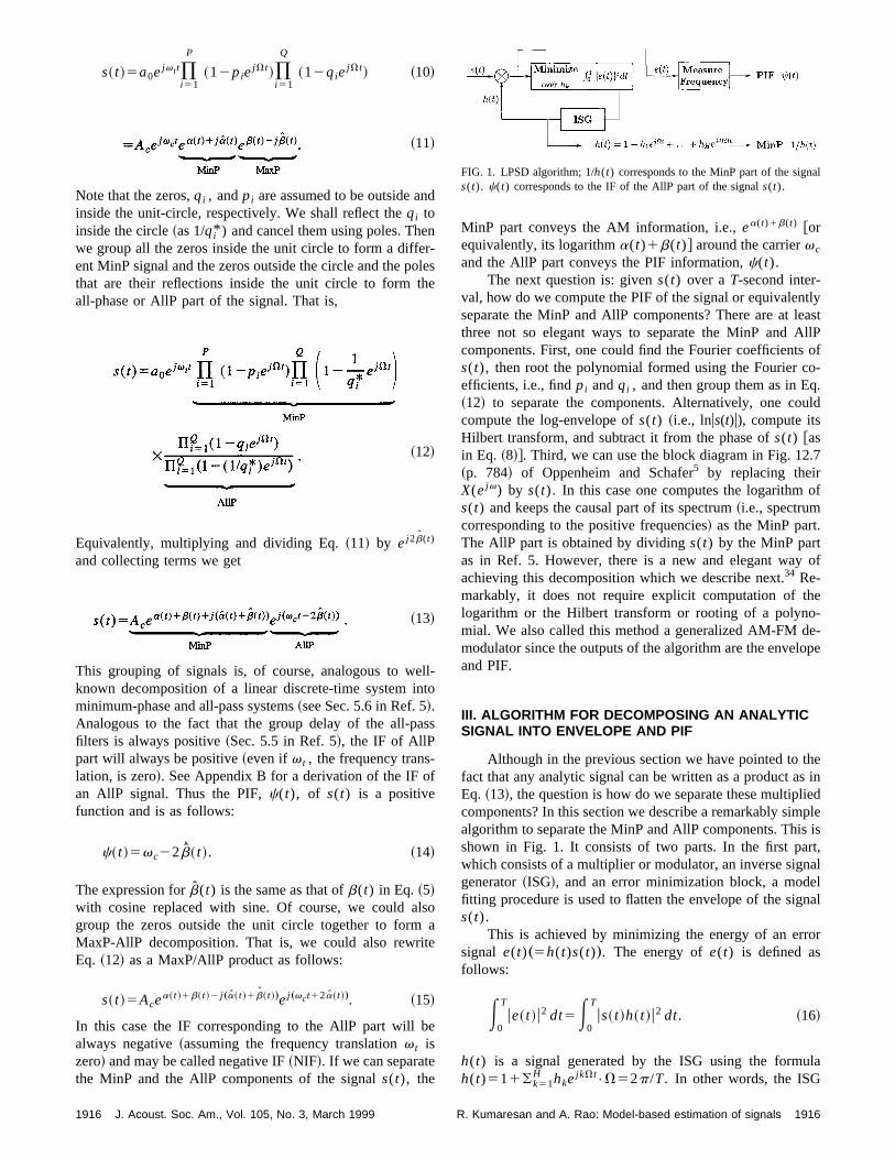
Although in the previous section we have pointed to tfact that any analytic signal can be written as a product aEq. ~13!, the question is how do we separate these multiplcomponents? In this section we describe a remarkably simalgorithm to separate the MinP and AllP components. Thishown in Fig. 1. It consists of two parts. In the first pawhich consists of a multiplier or modulator, an inverse signgenerator~ISG!, and an error minimization block, a modefitting procedure is used to flatten the envelope of the sigs(t).

This is achieved by minimizing the energy of an errsignal e(t)„5h(t)s(t)…. The energy ofe(t) is defined asfollows:

E0

T

ue~ t !u2 dt5E0

T

us~ t !h~ t !u2 dt. ~16!

h(t) is a signal generated by the ISG using the formh(t)511(k51

H hkejkVt

•V52p/T. In other words, the ISG

FIG. 1. LPSD algorithm; 1/h(t) corresponds to the MinP part of the signs(t). c(t) corresponds to the IF of the AllP part of the signals(t).


y

i-th

ins

nof

ef-

to

l-

f

we

n

lPas

t

gos

ns

nn-

ft

f

ofle-

e

bor-lso-

ofr.ti-

generates a low-pass periodic signal. The error energminimized by choosing the coefficients,hk . The reader whois familiar with model-based spectral analysis will immedately recognize the analogy between this method and‘‘autocorrelation method’’ of linear prediction.4,25 In the au-tocorrelation method, a discrete-time FIR filter, called anverse filter or prediction-error filter, with frequency responH(ej v) ~with first coefficient held at unity!, is used to flattenthe envelope of a spectrunX(ej v) of a sequencex(n) byminimizing the error*0

2puX(ej v)H(ej v)u2 dv. This is an ex-act analog of Eq.~16!. Analogous to the autocorrelatiomethod, the error in Eq.~16! is a measure of the flatnessthe envelope ofe(t). Also, minimizing the error in Eq.~16!amounts to performing linear prediction on the Fourier coficients of the signals(t) and hence we called it linear prediction in spectral domain or LPSD in earlier work.34 Thesignalh(t) may be called the ‘‘inverse signal’’ analogousthe inverse filter.

Similar to the MinP property of the prediction-error fiter used in linear prediction,25 minimizing *0

Tue(t)u2dt resultsin a h(t) that is a MinP signal~having all its signal zerosinside the unit circle!. This is true even if the envelope os(t) goes to zero at some points between 0 andT seconds,i.e., even if somepi or qi fall on the unit circle. The signifi-cance of this MinP property is that, as we already knoh(t)’s log-envelope and phase are Hilbert transforms. Bcause the error minimization is performed to flattens(t)’senvelope, if the value ofH is chosen sufficiently large, theh(t) will be given by

h~ t !'e2„a~ t !1b~ t !…e2 j „a~ t !1b~ t !…. ~17!

Thus, 1/h(t) is the desired approximation tos(t)’s MinPcomponent and hence the name ‘‘inverse signal’’ forh(t).Consequently, the error signale(t) will be e(t)

'Acej „vct22b(t)…, and hence is an approximation to the Al

component ofs(t). In the second part, denoted in Fig. 1‘‘measure frequency,’’ the PIF is computed ase(t)/ue(t)u ord/e(t)/dt. The next section describes the algorithm usedminimize the error*0

Tue(t)u2 dt.

A. LPSD algorithm using signal samples

In this section we present the details of the LPSD alrithm for computing the MinP and AllP approximationgiven the samples of the signals(t). The algorithm amountsto performing linear prediction on the discrete Fourier traform ~DFT! values of the signal samples. Lets@n# (n50,1,...,K), given by Eq.~1!, denote samples of the givesignal;K5N21. Let V52p/N be the assumed fundametal frequency. By replacingh(t) ande(t) by their respectivesampled versions, we have

e@n#5s@n#h@n#5s@n#1 (k51

H

hks@n#ejkVn, ~18!

which can be further expressed in matrix notation as


is

e

-e

-

,-

o

-

-

S s@0#s@1#]

s@K#

D 1S s@0# s@0# ¯ s@0#

ej Vs@1# ej 2Vs@1# ¯ ejHVs@1#

] ] � ]

ejKVs@K# ej 2KVs@K# ¯ ejKHVs@K#

D3S h1

h2

]

hH

D 5S e@0#e@1#]

e@K#

D . ~19!

If we let s, H, h, ande denote the vectors/matrices from leto right in Eq. ~19!, then the solution vector,h, that mini-mizeseTe5(n50

N21ue@n#u2, in Eq. ~19!, is given by

h52~HTH!21HTs. ~20!

Here T stands for conjugate-transpose and ( )21 denotesmatrix inverse operation. The matrix,H, can be further de-composed into a productH5SN3NXN3H :

H5S s@0# 0 ¯ ¯ 0

0 s@1# 0 ¯ 0

] ] � ] ]

0 0 ¯ 0 s@K#

DN3N

3S 1 1 ¯ 1

ej V ej 2V¯ ejHV

] ] � ]

ejKV ej 2KV¯ ejHKV

DN3H

. ~21!

In Eq. ~21!, observe thatS is a diagonal matrix consisting osignal samples whileX is essentially the DFT matrix. Usingthis decomposition, the solution vector,h, given by Eq.~20!,can be rewritten as

h52~XTSTSX!21XTSTs. ~22!

Clearly, the solution depends only on the magnitudes@n#. h@n# can then be reconstructed by substituting ements of the vectorh in h@n#511(k51

H hkejkVn

•sMinP@n#can then be computed as 1/h@n#; the log-envelope and phasof sMinP@n# correspond toa@n#1b@n# anda@n#1b@n#, re-

spectively. The positive frequency,vc22b@n#, can befound as the IF of the error signal,e@n#, using any standardIF estimator such as the phase difference between neighing samples.35 Instead, as mentioned earlier, we may aapply the LPSD algorithm again toe@n# @because the envelope of the first derivative ofe(t) is c(t), which is the PIF#.We call this step the second-stage LPSD.

The LPSD algorithm attempts to flatten the envelopethe signals(t) by using an adaptive amplitude demodulatoThis process not only eliminates the AM but also automacally removes from the phase ofs(t) a quantity equal to theHilbert transform of the log-envelope ofs(t). This is what


y,hexilsatetnP

nvanin

e

rean

045

r

ipe

deth

y

n

h-t

nob

th

Alsonof

of

landlinenal

.nofis

-theets

n-res

causes the IF ofe(t) to be positive. Instead, if we simpl‘‘clip’’ s(t), i.e., obtains(t)/us(t)u, then its phase derivativethe traditional IF, will not always be positive. Second, tMinP property ofh(t) guarantees that the envelope appromation 1/uh(t)u will never equal zero. Further, MinP signawill have their energy concentrated over a relatively smregion in the spectral domain analogous to a MinP filwhich has its impulse response peaking close to origin. Ialso possible to use the LPSD algorithm to achieve a MiMaxP ~instead of MinP-AllP! decomposition ofs(t). Sepa-ration of these components may also be viewed as decolution of their spectra in the frequency domain. Third,important advantage of the LPSD algorithm is thatachieves the separation of the MinP and AllP componewithout explicitly rooting a polynomial or computing thlogarithm or Hilbert transform of the signals(t).

B. Simulation results

We now provide results of applying the LPSD proceduto decompose synthetic signals. It will be followed byexample of a speech signal.

1. Synthetic signals

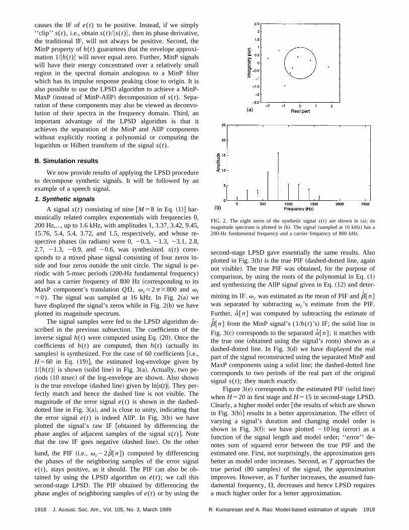
A signal s(t) consisting of nine@M58 in Eq. ~1!# har-monically related complex exponentials with frequencies200 Hz,..., up to 1.6 kHz, with amplitudes 1, 3.37, 3.42, 9.15.76, 5.4, 5.4, 3.72, and 1.5, respectively, and whosespective phases~in radians! were 0,20.3, 21.3, 23.1, 2.8,2.7, 21.3, 20.9, and20.6, was synthesized.s(t) corre-sponds to a mixed phase signal consisting of four zerosside and four zeros outside the unit circle. The signal isriodic with 5-msec periods~200-Hz fundamental frequency!and has a carrier frequency of 800 Hz~corresponding to itsMaxP component’s translationQV, vc52p3800 andv t

50). The signal was sampled at 16 kHz. In Fig. 2~a! wehave displayed the signal’s zeros while in Fig. 2~b! we haveplotted its magnitude spectrum.

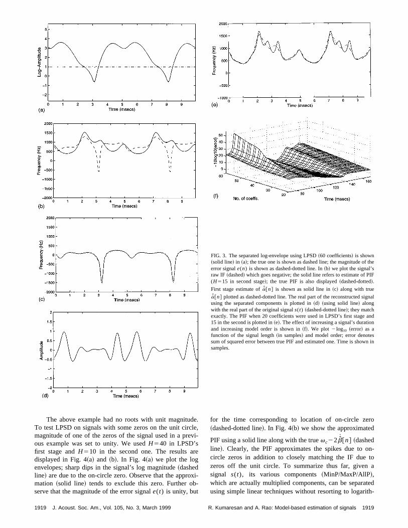
The signal samples were fed to the LPSD algorithmscribed in the previous subsection. The coefficients ofinverse signalh(t) were computed using Eq.~20!. Once thecoefficients ofh(t) are computed, thenh(t) ~actually itssamples! is synthesized. For the case of 60 [email protected].,H560 in Eq. ~19!#, the estimated log-envelope given b1/uh(t)u is shown~solid line! in Fig. 3~a!. Actually, two pe-riods ~10 msec! of the log-envelope are shown. Also showis the true envelope~dashed line! given by lnus(t)u. They per-fectly match and hence the dashed line is not visible. Tmagnitude of the error signale(t) is shown in the dasheddotted line in Fig. 3~a!, and is close to unity, indicating thathe error signale(t) is indeed AllP. In Fig. 3~b! we haveplotted the signal’s raw IF@obtained by differencing thephase angles of adjacent samples of the signals(t)#. Notethat the raw IF goes negative~dashed line!. On the other

hand, the PIF~i.e., vc22b@n#) computed by differencingthe phases of the neighboring samples of the error sige(t), stays positive, as it should. The PIF can also betained by using the LPSD algorithm one(t); we call thissecond-stage LPSD. The PIF obtained by differencingphase angles of neighboring samples ofe(t) or by using the


-

llris-

o-

tts

,,e-

n--

-e

e

al-

e

second-stage LPSD gave essentially the same results.plotted in Fig. 3~b! is the true PIF~dashed-dotted line, againot visible!. The true PIF was obtained, for the purposecomparison, by using the roots of the polynomial in Eq.~1!and synthesizing the AllP signal given in Eq.~12! and deter-

mining its IF.vc was estimated as the mean of PIF andb@n#was separated by subtractingvc’s estimate from the PIF.Further, a@n# was computed by subtracting the estimate

b@n# from the MinP signal’s (1/h(t)’s! IF; the solid line inFig. 3~c! corresponds to the separateda@n#; it matches withthe true one~obtained using the signal’s roots! shown as adashed-dotted line. In Fig. 3~d! we have displayed the reapart of the signal reconstructed using the separated MinPMaxP components using a solid line; the dashed-dottedcorresponds to two periods of the real part of the origisignals(t); they match exactly.

Figure 3~e! corresponds to the estimated PIF~solid line!whenH520 in first stage andH515 in second-stage LPSDClearly, a higher model order@the results of which are showin Fig. 3~b!# results in a better approximation. The effectvarying a signal’s duration and changing model ordershown in Fig. 3~f!: we have plotted210 log ~error! as afunction of the signal length and model order; ‘‘error’’ denotes sum of squared error between the true PIF andestimated one. First, not surprisingly, the approximation gbetter as model order increases. Second, asT approaches thetrue period~80 samples! of the signal, the approximationimproves. However, asT further increases, the assumed fudamental frequency,V, decreases and hence LPSD requia much higher order for a better approximation.

FIG. 2. The eight zeros of the synthetic signals(t) are shown in~a!; itsmagnitude spectrum is plotted in~b!. The signal~sampled at 16 kHz! has a200-Hz fundamental frequency and a carrier frequency of 800 kHz.


the

IF

ignal

andn

swn in

FIG. 3. The separated log-envelope using LPSD~60 coefficients! is shown~solid line! in ~a!; the true one is shown as dashed line; the magnitude oferror signale(n) is shown as dashed-dotted line. In~b! we plot the signal’sraw IF ~dashed! which goes negative; the solid line refers to estimate of P(H515 in second stage!; the true PIF is also displayed~dashed-dotted!.

First stage estimate ofa@n# is shown as solid line in~c! along with true

a@n# plotted as dashed-dotted line. The real part of the reconstructed susing the separated components is plotted in~d! ~using solid line! alongwith the real part of the original signals(t) ~dashed-dotted line!; they matchexactly. The PIF when 20 coefficients were used in LPSD’s first stage15 in the second is plotted in~e!. The effect of increasing a signal’s duratioand increasing model order is shown in~f!. We plot 2 log10 ~error! as afunction of the signal length~in samples! and model order; error denotesum of squared error between true PIF and estimated one. Time is shosamples.

dele

ev

re

oxb-

ro

on-toa

tedth-

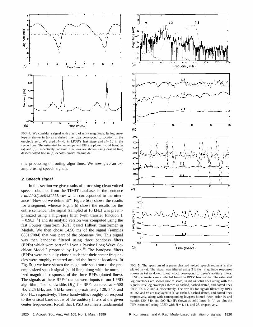
The above example had no roots with unit magnituTo test LPSD on signals with some zeros on the unit circmagnitude of one of the zeros of the signal used in a prous example was set to unity. We usedH540 in LPSD’sfirst stage andH510 in the second one. The results adisplayed in Fig. 4~a! and ~b!. In Fig. 4~a! we plot the logenvelopes; sharp dips in the signal’s log magnitude~dashedline! are due to the on-circle zero. Observe that the apprmation ~solid line! tends to exclude this zero. Further oserve that the magnitude of the error signale(t) is unity, but


.,i-

i-

for the time corresponding to location of on-circle ze~dashed-dotted line!. In Fig. 4~b! we show the approximated

PIF using a solid line along with the truevc22b@n# ~dashedline!. Clearly, the PIF approximates the spikes due tocircle zeros in addition to closely matching the IF duezeros off the unit circle. To summarize thus far, givensignal s(t), its various components~MinP/MaxP/AllP!,which are actually multiplied components, can be separausing simple linear techniques without resorting to logari


x

en

r-

he

alte-

en.re

S

nonenen

dis-

.ated

linesFses

vethe

ne

mic processing or rooting algorithms. We now give an eample using speech signals.

2. Speech signal

In this section we give results of processing clean voicspeech, obtained from the TIMIT database, in the sentetrain/dr3/fcke0/si1111.wavwhich corresponded to the utteance ‘‘How do we define it?’’ Figure 5~a! shows the resultsfor a segment, whereas Fig. 5~b! shows the results for theentire sentence. The signal~sampled at 16 kHz! was preem-phasized using a high-pass filter~with transfer function 120.98z21) and its analytic version was computed using tfast Fourier transform~FFT! based Hilbert transformer inMatlab. We then chose 14.56 ms of the signal~samples6851:7084! that was part of the phoneme /iy/. This signwas then bandpass filtered using three bandpass fi~BPFs! which were part of ‘‘Lyon’s Passive Long Wave Cochlear Model’’ proposed by Lyon.36 The bandpass filters~BPFs! were manually chosen such that their center frequcies were roughly centered around the formant locationsFig. 5~a! we have shown the magnitude spectrum of the pemphasized speech signal~solid line! along with the normal-ized magnitude responses of the three BPFs~dotted lines!.The signals at these BPFs’ output were inputs to our LPalgorithm. The bandwidths (Bc) for BPFs centered at'500Hz, 2.25 kHz, and 5 kHz were approximately 120, 340, a900 Hz, respectively. These bandwidths roughly correspto the critical bandwidths of the auditory filters at the givcenter frequencies. Recall that LPSD assumes a fundam

FIG. 4. We consider a signal with a zero of unity magnitude. Its log enlope is shown in~a! as a dashed line; dips correspond to location ofon-circle zero. We usedH540 in LPSD’s first stage andH510 in thesecond one. The estimated log envelope and PIF are plotted~solid lines! in~a! and ~b!, respectively; original functions are shown using dashed lidashed-dotted line in~a! denotes error’s magnitude.


-

dce

lrs

-In-

D

dd

tal

FIG. 5. The spectrum of a preemphasized voiced speech segment isplayed in ~a!. The signal was filtered using 3 BPFs@magnitude responsesshown in ~a! as dotted lines# which correspond to Lyon’s auditory filtersLPSD parameters were selected based on BPFs’ bandwidths. The estimlog envelopes are shown~not to scale! in ~b! as solid lines along with thesignals’ true log envelopes shown as dashed, dashed-dotted, and dottedfor BPFs 1, 2, and 3, respectively. The raw IFs for signals filtered by BP#1, #2, and #3 are displayed in~c! as dashed, dashed-dotted, and dotted linrespectively, along with corresponding lowpass filtered~with order 50 andcutoffs 120, 340, and 900 Hz! IFs shown as solid lines. In~d! we plot thePIFs estimated using LPSD withH54, 11, and 28, respectively.

-

;


efo

ms,-st

rg

thenve

fild

igve

ed

hara

bv

oI

begn

, in

.reth

erspo-ap-ion.6.

ockot

os

, l

frerect

is

g-three

thePFs.ries

frequency,V, of 2p/N; this corresponds to 32 Hz for thpresent example. Having specified a certain bandwidthenvelope approximation, one can compute the algorithmodel order asH52pBc /V. Based on these calculationwe chose LPSD model orders,H, to be 12, 33, and 84, corresponding to three times the critical bandwidths for firstage envelope approximation. The values ofH were set to 4,11, and 28 for approximating the PIFs in second-stage pcessing. One may also keepH fixed and vary the processininterval for each BPF proportional to 1/Bc . Our goal was notto parsimoniously describe the signal but to demonstratethe carrier frequency and the modulations carry sufficiinformation to describe the signal. The estimated log enlopes are shown in Fig. 5~b! as solid lines~not to scale! alongwith the signal’s Hilbert envelopes for each of the threeters~dashed, dashed-dotted, and dotted for BPFs 1, 2, anrespectively!. The raw IFs~obtained by phase-differencing!for signals filtered by the three BPFs are displayed in F5~c! as dashed, dashed-dotted, and dotted lines, respectialong with corresponding lowpass filtered~with order 50 andcutoffs 120, 340, and 900 Hz! IFs shown as solid lines. ThPIFs resulting from second-stage processing are depicteFig. 5~d!.

Based on earlier discussions we can see that the sspikes in raw log-envelopes and most of the spikes inIFs ~especially for signals at output of BPFs 2 and 3! are dueto signal zeros very close to the unit circle; the latter maycaused by neighboring peaks in the signal’s spectral enlope ~or neighboring formants!. Further, the raw IFs also gnegative at times. In general, the raw log-envelopes andare highly fluctuating quantities. Clearly, the LPSD mayviewed as a technique to compute a signal’s envelope’s lorithm. The IF approximated by LPSD has two distinct advatages over techniques that merely filter the raw IF. Firstthe absence of on-circle zeros, it is always positive. Secoit approximates the typically impulsive IF better~due to theall-pole model assumption! as opposed to lowpass filtered IF

When a composite signal consists of many spectralgions of interest which are time-varying, as in speech,

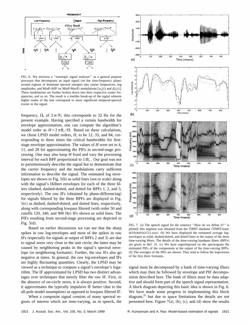
FIG. 6. We envision a ‘‘tonotopic signal analyzer’’ as a general purpprocessor that decomposes an input signal~on the time-frequency plane!around regions of dominant spectral energies into carrier frequenciesamplitudes, and MinP-AllP~or MinP-MaxP! modulations@ak(t) andbk(t)#.These modulations are further broken down into their respective centerquencies, and so on. The result is a treelike break-up of the signal whhigher nodes of the tree correspond to more significant temporal-speevents in the signal.


r’s

-

o-

att-

-3,

.ly,

in

rpw

ee-

Fs

a--nd,

-e

signal must be decomposed by a bank of time-varying filtwhich may then be followed by envelope and PIF decomsition described here. The bank of filters must be data adtive and should form part of the speech signal representatA block diagram depicting this basic idea is shown in Fig.We have made some progress in implementing this bldiagram,31 but due to space limitations the details are npresented here. Figure 7~a!, ~b!, ~c!, and~d! show the results

e

og

e-in

ral

FIG. 7. ~a! The speech signal for the sentence ‘‘How do we define it?’’plotted; this segment was obtained from the TIMIT database~TIMIT/train/dr3/fcke0/si1111.wav!. ~b! We have displayed the estimated average loenvelopes as solid, dashed-dotted, and dotted lines at the output of thetime-varying filters. The details of the time-varying bandpass filters~BPFs!are given in Ref. 31.~c! We have superimposed on the spectrogramestimated PIFs of the components at the output of the time-varying B~d! The averages of the PIFs are shown. They tend to follow the trajectoof the first three formants.


?’o

pr

p

poa

-m

cle

nr’sbnoua

P/eiin

eifiPd

se

thi

anu

ny

-

eb

ae-ise

Na0

aller

n-

tarysefor

-

al

e of

of processing the entire sentence ‘‘How do we define itusing this decomposition. We may call this approach ‘‘Tontopic Signal Analysis~TSA!,’’ since the procedure not onlyattempts to track the formant center frequencies but alsovides the details of modulations~the a and b! about thosefrequencies. Reference 31 provides several such speechcessing examples.

IV. DISCUSSION

In this paper our main accomplishment is the decomsition of an analytic signal into two analytic signals usingsimple ~LPSD! algorithm. Decomposition of analytic functions of a complex variable has been studied in systetheory and filter design since the days of Henrik Bode37 inthe 1930s. However, much of that work dealt with frequenresponses, i.e., frequency is viewed as a complex variabs~continuous-time systems! or z ~discrete-time systems!.Cepstrum-related research5 may be viewed as an extensioof this work. Voelcker’s contribution, which extends Gabowork,7 is that he recognized that analytic functions couldused for studying the relationships between phase and elope of signals by treating time as a complex variable. Toknowledge, Voelcker did not attempt to decompose signinto MinP and MaxP or AllP components. The MinP/MaxAllP decomposition was, perhaps, first done by Oppenhand colleagues~see Ch. 12 in Ref. 5, and references there!.However, their decomposition was achieved by rootingpolynomial or computing logarithm/log-derivative in thz-transform or frequency domain. In contrast, the signcance of our result is that the MinP-AllP or MinP-Maxdecomposition is achieved using an elegant adaptivemodulator without rooting, Hilbert transformation, or phaunwrapping, directly from the given signals(t). A similarprocedure can be developed for the frequency domainwell. The primary difference between our approach andcepstrum analysis is that we explore the signal’s logarithmthe time domain which yields a physically acceptable qutity like the positive instantaneous frequency. This helpsin characterizing the IF of signals which consist of macomponents such as a speech formant. The average PIF~i.e.,the carrier frequency! indicates the place-location of a signal’s spectral concentration.

Unfortunately, in this paper, we still need to form thanalytic signal before the proposed decomposition canachieved. That is, since in practice only real-valued signare available for processing, one has to compute its Hilbtransform. In more recent work38 we have proposed an algorithm which avoids computation of the analytic signal. Itpossible to obtain the envelope and PIF directly from the rsignal under certain restrictions.

ACKNOWLEDGMENT

This research was supported by a grant from thetional Science Foundation under Grant No. CCR-980405


’-

o-

ro-

-

s

y

eve-rls

m

a

-

e-

asen-s

elsrt

al

-.

APPENDIX A: MINIMUM AND MAXIMUM PHASESIGNALS

An elementary signal,23 e(t), is defined as

e~ t !512pej Vt, ~A1!

wherep5upuej u. If upu,1 thene(t) is called a MinP signal,since no other signal with the same envelope has a smphase angle. Observe thatue(t)u.0. Taking the natural loga-rithm of both sides and using the series expansion, ln(12y)5(k51

` (2yk/k), we get

ln~12pej Vt!5 (k51

`2pke2 jkVt

k. ~A2!

After exponentiating both sides, we get the following idetity:

12pej Vt5expS (k51

`2upuk

kcos~kVt1ku!

1 j (k51

`2upuk

ksin~kVt1ku!D . ~A3!

From the above expression we note that for an elemenMinP signal,e(t), the logarithm of its envelope and its phaangle are related through the Hilbert transform. Similarly,an elementary MaxP signal (12qej Vt) where q5uquej f,uqu.1, we get the following identity:

12qej Vt5~2qej Vt!expS (k51

`2u1/quk

kcos~kVt1kf!

2 j (k51

`2u1/quk

ksin~kVt1kf!D . ~A4!

The key difference between Eqs.~A3! and~A4! is the changein the sign of the phase function.

Using the above identities in Eq.~2! yields

sMinP~ t !5ea~ t !1 j a~ t ! ~A5!

and

sMaxP~ t !5A0eb~ t !1 j ~v0t2b~ t !!, ~A6!

where

a~ t !5 (k51

`

(i 51

P

2upi uk

kcos~kVt1ku i ! ~A7!

and

b~ t !5 (k51

`

(i 51

Q

21/uqi uk

kcos~kVt1kf i !. ~A8!

Thus s(t) as described in Eq.~2! can be compactly represented as

s~ t !5Acej vctea~ t !1 j a~ t !eb~ t !2 j b~ t !, ~A9!

whereAc corresponds to the overall amplitude of the signandvc denotes its ‘‘carrier’’ frequency.vc is equal toQVplus any arbitrary frequency translation that the signals(t)may have been subjected to. The log-envelope and phas


edthecae,al

ee

ai

s

s

d

’’toals

e,

dis-F

e-

ear

ionss,’’

E

nalss.

of

s(t) are expressed in terms ofa(t) andb(t) as

lnus~ t !u5a~ t !1b~ t !1 ln Ac ~A10!

and

/s~ t !5vct1a~ t !2b~ t !, ~A11!

respectively. The above expressions can be a useful pgogical tool in explaining phase-envelope relationships insignal as well as systems domains. For instance, the wknown results in Ref. 39, where one attempts to reconstrusignal from either phase or magnitude information, may eily be explained using the above expressions. For exampla pair of roots ofs(t) occurs in complex conjugate reciproclocations, i.e.,pi51/qi* , then thei th term in the summationin Eqs.~A7! and~5! are identical and hence vanish from thexpression for phase in Eq.~A11!. Hence, in this case, phasdoes not uniquely specify the signals(t). This is essentiallytheorem 1 in Ref. 39, which is stated in the systems domSimilarly if pi521/qi* , then from Eq.~A10! we see thatmagnitude alone is not sufficient to specify a signals(t). Ingeneral, both phase and envelope are required to repres(t).

The instantaneous frequency~IF! of s(t) is the deriva-

tive of the phase ofs(t) and is simplyvc1 a(t)2 b(t)~where the dot stands for the first derivative!, i.e., it consistsof a dc~corresponding to carrier frequency! and a sum of IFsof s(t)’s MinP and MaxP components. Thus we have

d/s~ t !

dt5vc2VF (

k51

` S (i 51

P

upi uk cos~kVt1ku i !

2(i 51

Q

u1/qi uk cos~kVt1kf i !D G . ~A12!

Clearly, the spectrum ofs(t)’s IF @given by Eq.~A12!# con-tains an infinite number of harmonic components~V beingthe fundamental frequency!. A closed-form expression for IFis obtained by summing Eq.~A12! as

d/s~ t !/dt

5vc2VF(i 51

P upi u~cos~Vt1u i !2upi u!122up1ucos~Vt1u i !1up1u2

2(i 51

Q u1/qi u~cos~Vt1f i !2u1/qi u!122u~1/qi !ucos~Vt1f i !1u~1/qi !u2G . ~A13!

The above reveals thats(t)’s IF tends to6` whenever oneor more of its zeros tend to lie on the unit circle~see Ref. 31for details!. All these results were known to Voelcker.

APPENDIX B: SIGNALS WITH POSITIVEINSTANTANEOUS FREQUENCY

Consider a signal,z(t), which is a ratio of two signals afollows:

z~ t !512qej Vt

12 ~1/q* !ej Vt ; ~B1!


a-ell-t as-if

n.

ent

‘‘ * ’’ denotes complex conjugation,q5uquej f, and uqu.1.Rearranging the numerator we have

z~ t !52qej Vt12~1/q!e2 j Vt

12~1/q* !ej Vt . ~B2!

Simplifying the above equation, we find thatz(t)’s envelopeis a constant~equal touqu! for all time, t, and that its phaseangle is

/z~ t !5Vt1p1f12(k51

` u1/quk

ksin~kVt1kf!. ~B3!

Taking the first derivative of/z(t), its IF can be expresseas

d/z~ t !

dt5VS 112(

k51

` U1qUk

cos~kVt1kf!D . ~B4!

Since the right side of Eq.~B4! is V(12u1/qu2)u12(1/q* )ej Vtu22 and is analogous to a ‘‘power spectrum,z(t)’s IF is always positive. We may generalize this resultthe case of a signal consisting of a product of rational signas in Eq.~B2!, i.e., z(t) of form

z~ t !5)i 51

L12qie

j Vt

12~1/qi* !ej Vt . ~B5!

Since the phase angle contribution due to each of theL termsin the above equation adds up, the corresponding IF is

d/z~ t !

dt5V(

i 51

L S 112(k51

` U 1

qiUk

cos~kVt1kf i !D .

~B6!

Since each of theL terms in the above summation is positivwe claim that the final IF given by Eq.~B6! is positive.These results are analogous to the results well known increte time all-pass~AP! systems, where the equivalent of Iis the group delay;40 our derivation is slightly different thanthe one given in Oppenheim and Schafer.5

1L. Cohen, ‘‘Time-frequency distributions—A review,’’ Proc. IEEE77,941–981~1989!.

2F. Hlawatsch and G. F. Boudreaux-Bartels, ‘‘Linear and quadratic timfrequency signal representations,’’ IEEE ASSP Magazine9, 21–67~April1992!.

3B. S. Atal and S. L. Hanauer, ‘‘Speech analysis and synthesis by linprediction of the speech wave,’’ J. Acoust. Soc. Am.50, 637–655~1971!.

4J. I. Makhoul, ‘‘Linear prediction: A tutorial review,’’ Proc. IEEE63,561–580~1975!.

5A. V. Oppenheim and R. W. Schafer,Discrete-Time Signal Processing~Prentice-Hall, Englewood Cliffs, NJ, 1989!.

6S. Davis and P. Mermelstein, ‘‘Comparison of parametric representatfor monosyllabic word recognition in continuously spoken sentenceIEEE Trans. Acoust., Speech, Signal Process.4, 357–366~1980!.

7D. Gabor, ‘‘Theory of communication,’’ Proc. IEE93, 429–457~1946!.8J. Dugundji, ‘‘Envelopes and preenvelopes of real waveforms,’’ IRTrans. Inf. Theory4, 53–57~1958!.

9A. Papoulis,The Fourier Integral and its Applications~McGraw-Hill,New York, 1962!.

10L. Cohen,Time-Frequency Analysis~Prentice-Hall, Englewood Cliffs, NJ,1995!.

11P. Maragos, T. F. Quatieri, and J. F. Kaiser, ‘‘Energy separation in sigmodulations with applications to speech,’’ IEEE Trans. Signal Proce41, 3024–3051~1993!.

12F. Casacuberta and E. Vidal, ‘‘A nonstationary model for the analysis


ce

ng

cy

o

er-

ys

ve

mns

o-

E

e-

e-

n

s ofing

ted.udi-I,

tic

ess-

ns.

.,

e of

on

transient speech signals,’’ IEEE Trans. Acoust., Speech, Signal Pro35, 226–228~1987!.

13T. F. Quatieri, T. E. Hanna, and G. C. O’Leary, ‘‘Am-fm separation usiauditory motivated filters,’’ IEEE Trans. Speech Audio Process.5, 465–480 ~1997!.

14P. J. Loughlin and B. Tacer, ‘‘On the amplitude- and frequenmodulation decomposition of signals,’’ J. Acoust. Soc. Am.100~3!,1594–1601~1996!.

15J. L. Flanagan, ‘‘Parametric coding of speech spectra,’’ J. Acoust. SAm. 68, 412–419~1980!.

16A. V. Oppenheim, R. W. Schafer, and T. G. Stockham, ‘‘Nonlinear filting of multiplied and convolved signals,’’ Proc. IEEE56, 1264–1291~1968!.

17L. Mandel, ‘‘Interpretation of instantaneous frequencies,’’ Am. J. Ph42, 840–846~1974!.

18E. Bedrosian, ‘‘The analytic signal representation of modulated waforms,’’ Proc. IRE50, 2071–2076~1962!.

19J. Shekel, ‘‘Instantaneous frequency,’’ Proc. IRE41, 548–548~1953!.20D. Vakman, ‘‘On the analytic signal, the Teager-Kaiser energy algorith

and other methods for defining amplitude and frequency,’’ IEEE TraSignal Process.44, 791–797~1996!.

21M. Poletti, ‘‘The homomorphic analytic signal,’’ IEEE Trans. Signal Prcess.45, 1943–1953~1997!.

22B. Picinbono, ‘‘On instantaneous amplitude and phase of signals,’’ IETrans. Signal Process.45, 552–560~1997!.

23H. B. Voelcker, ‘‘Towards a unified theory of modulation part I: Phasenvelope relationships,’’ Proc. IEEE54, 340–354~1966!.

24H. B. Voelcker, ‘‘Towards a unified theory of modulation part II: Phasenvelope relationships,’’ Proc. IEEE54„5…, 735–755~1966!.

25S. M. Kay, Modern Spectral Estimation: Theory and Applicatio~Prentice-Hall, Englewood Cliffs, NJ, 1987!.

26Auditory Computation, edited by H. L. Hawkins, T. A. McMullen, A. N.


ss.

-

c.

.

-

,.

E

Popper, and R. R. Fay~Springer-Verlag, New York, 1996!.27S. Khanna and M. C. Teich, ‘‘Spectral characteristics of the response

primary auditory-nerve fibers to frequency modulated signals,’’ HearRes.39, 143–158~1989!.

28L. B. Jackson,Signals, Systems, and Transforms~Addison-Wesley, Read-ing, MA, 1991!.

29Entire Functions, edited by R. P. Boas~Academic, New York, 1954!.30A. G. Requicha, ‘‘Contributions to a zero based theory of band limi

signals,’’ Ph.D. thesis, University of Rochester, Rochester, NY, 197031A. Rao, ‘‘Signal analysis using product expansions inspired by the a

tory periphery,’’ Ph.D. thesis, University of Rhode Island, Kingston, RJune 1997.

32R. Nevanlinna,Analytic Functions~Springer-Verlag, Berlin, 1970!.33W. Rudin,Real and Complex Analysis~McGraw-Hill, New York, 1987!.34R. Kumaresan and A. Rao, ‘‘An algorithm for decomposing an analy

signal into AM and positive FM components,’’ inProceedings of theIEEE International Conference on Acoustics, Speech and Signal Procing, Seattle, WA, May 1998, pp. III:1561–1564.

35S. M. Kay, ‘‘A fast and accurate single frequency estimator,’’ IEEE TraSpeech Audio Process.37, 1987–1990~1989!.

36M. Slaney, ‘‘Auditory toolbox,’’ Tech. Rep. 45, Apple Computer, Inc1994.

37Network Analysis and Feedback Amplifier Design, edited by H. W. Bode~Van Nostrand, Princeton, 1945!.

38R. Kumaresan, ‘‘An inverse signal approach to computing the envelopa real valued signal,’’ IEEE Signal Process. Lett.October, 256–259~1998!.

39M. H. Hayes, J. S. Lim, and A. V. Oppenheim, ‘‘Signal reconstructifrom phase or magnitude,’’ IEEE Trans. Speech Audio Process.28, 672–680 ~1980!.

40E. A. Robinson,Time Series Analysis and Applications~Goose Pond,Houston, 1981!.


Documents

Model-based approach to envelope and positive …saito/data/phase/kumaresan-rao.pdfModel-based approach to envelope and positive instantaneous frequency estimation of signals with