Modeling and Optimization of Complex BuildingEnergy Systems with Deep Neural Networks

Yize Chen, Yuanyuan Shi and Baosen Zhang∗Department of Electrical Engineering, University of Washington, Seattle, WA, USA

{yizechen, yyshi, zhangbao}@uw.edu

Abstract—Modern buildings encompass complex dynamics ofmultiple electrical, mechanical, and control systems. One of thebiggest hurdles in applying conventional model-based optimiza-tion and control methods to building energy management isthe huge cost and effort of capturing diverse and temporallycorrelated dynamics. Here we propose an alternative approachwhich is model-free and data-driven. By utilizing high volume ofdata coming from advanced sensors, we train a deep RecurrentNeural Networks (RNN) which could accurately represent the op-eration’s temporal dynamics of building complexes. The trainednetwork is then directly fitted into a constrained optimizationproblem with finite horizons. By reformulating the constrainedoptimization as an unconstrained optimization problem, we useiterative gradient descents method with momentum to findoptimal control inputs. Simulation results demonstrate proposedmethod’s improved performances over model-based approach onboth building system modeling and control.

Index Terms—Building energy management, deep learning,gradient algorithms, HVAC systems

I. INTRODUCTION

According to a recent United Nations Environment Pro-gramme (UNEP) report, buildings are responsible for 40% ofthe global energy consumption [1]. Consequently, managingthe energy consumption of buildings has significant econom-ical, social, and environmental impacts, and has receivedmuch attention from researchers. Many approaches have beenproposed to control building systems (e.g., commercial andoffice buildings, data centers) for energy efficiency, such asnonlinear adaptive control, Model Predictive Control (MPC)and decentralized control for building heating, ventilation,and air conditioning (HVAC) systems [2], [3], [4]. However,most previous research on building energy management areeither based on the detailed physics model of buildings [5] orsimplified RC circuit models [2], [3], [6]. The former ofteninvolves tedious and complex modeling processes with a hugenumber of variables and parameters, whereas the latter cannotfully capture the long term dynamics of large commercialbuildings.

With the advance of sensing, communication and com-puting, detailed operation data are being collected for manybuildings. These data along with future weather forecasts canbe utilized for data-driven real-time optimization approaches.In [7], the authors developed a data predictive control methodto replace the traditional MPC controller by using data tobuild a regression tree that represent the dynamical modelfor a building. However, regression trees still results in alinear model that can be far away from the true dynamics

of building systems. While in [8], [9], reinforcement learningwas proposed to learn control policies without any explicitmodeling assumptions, but computational costs for searchingthrough large state and action spaces is hight. Ill-definedreward functions (e.g., sparse, noisy and delayed rewards)could also prevent reinforcement learning algorithm findingthe optimal control solutions [10]. Furthermore, large com-mercial buildings may have quality of service constraints thatprevent the deep exploration of some states in reinforcementlearning.

Building RunningPro�ile tX

Deep Recurrent Neural Network

Energy Consumption

tP

Constrained Optimization on

Optimal Control Inputs

...

t-nP

t-n+1P

( , )T t tRNN X H

t+n-1P

t+nP

...

ctX

( ,..., )tRNN t T tP f X X−=

( , )T t tRNN X H

OriginalControl Inputs c

tX

*ctX

(a). RNN Fitting

(b). Inputs Optimization

*tP

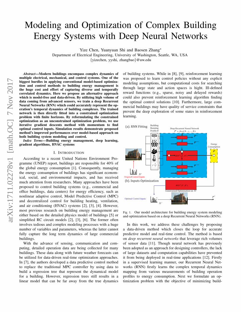
Fig. 1. Our model architecture for building energy system modelingand optimization based on a deep Recurrent Neural Networks (RNN).

In this work, we address these challenges by proposinga data-driven method which closes the loop for accuratepredictive model and real-time control. The method is basedon deep recurrent neural networks that leverage rich volumesof sensor data [11]. Though neural network has previouslybeen adopted as an approach for designing controllers, the lackof large datasets and computation capabilities have preventedit from being deployed in real-time applications [12]. Firstlyin a supervised learning manner, our Recurrent Neural Net-works (RNN) firstly learns the complex temporal dynamicsmapping from various measurements of building operationprofiles to energy consumption. Next we formulate an op-timization problem with the objective of minimizing build-

arX

iv:1

711.

0227

8v1

[m

ath.

OC

] 7

Nov

201

7

ing energy consumption, which is subject to RNN-modeledbuilding dynamics as well as physical constraints over a finitehorizon of time. To solve the constrained optimization problemin a block-splitting approach, we take iterative gradient descentsteps on the set of controllable inputs (e.g., zone temperaturesetpoints, heat rejected/added into each zone) at the currenttimestep. It thus finds the control inputs for each timestep.Fig. 1 illustrates our model framework. Our approach doesnot need analysis on complex interactions within conduction,convection or radiation processes. In addition, it can be easilyscaled up to large buildings and distributed algorithms.

The main contributions of our paper are:• We model the building energy dynamics using recurrent

neural networks, which leverages large volumes of datato represent the complex dynamics of buildings.

• We propose an input/output optimization algorithm whichefficiently find the optimal control inputs for the modelrepresented by RNN.

• The proposed modeling and optimization approachesopen door to the integration of complex system dynamicsmodeling and decision-making.

The contents of the paper are as follows. The rolling horizoncontrol problem formulation and model-based method arefirstly presented in Section. II. In Section. III we show thedesign of a deep RNN which models the dynamics of complexbuilding systems. We then reformulate the control problemas an unconstrained optimization problem, and propose thealgorithm to find optimal control inputs in Section. IV. Fi-nally, simulation results on large building HVAC system areevaluated and compared with model-based control method inSection. V.

II. PROBLEM FORMULATION & PRELIMINARIES

A. Problem FormulationWe consider a building energy system which includes sev-

eral subsystems and zones with potentially complex interac-tions between them. No information about the exact systemdynamics is known. At time t, we are provided with thebuilding’s running profile Xt := [Xuc

t ,Xct ,X

phyt ]T , where

Xuct denotes a collection of uncontrollable measurements such

as zone temperature measurements, system node temperaturemeasurements, lighting schedule, in-room appliances schedule,room occupancies and etc; and Xc

t denotes a collection ofcontrollable measurements such as zone temperature setpoints,appliances working schedule and etc; Xphy

t denotes the set ofphysical measurements or forecasts values, such as dry bulbtemperature, humidity and radiation volume. There are somephysical constraints on some of Xc

t and Xuct , for example

the temperature setpoints as well as real measurements shouldnot fall out of users’ comfort regions. Without loss of gen-erality, we denote the constraints as Xc

t ≤ Xct ≤ X

c

t andXuct ≤ Xuc

t ≤ Xuc

t . Building System operators have a groupof past running profile X = {Xt} along with the collectionof energy consumption metering at each time step P = {Pt}.

We are interested in firstly learning a modelf(Xt−T , ...,Xt) = Pt, where f(·) denotes the predictive

model with known parameters representing building’s physicaldynamics. f(·) maps past T timestep’s running profile toenergy consumption at timestep t.

With a model f(·) representing the building dynamics, weformulate an optimal finite-horizon predictive control prob-lem, and propose an efficient algorithm to find the group ofoptimal control inputs Xc∗

t . At timestep t, the control inputXct minimizes the energy consumption of the building for

future T steps. Meanwhile, previous T steps’ control inputswould affect current energy consumption. The objective ofthe controller is to minimize the energy consumption with arolling horizon T , while maintaining some variables withincomfortable intervals. Mathematically, we formulate the gen-eral control problem as

minimizeXct ,...,X

ct+T

T∑τ=0

P 2t+τ (1a)

subject to Pt+τ = f(Xt−T+τ , ...,Xt+τ ),∀τ (1b)

Xct+τ ≤ Xc

t+τ ≤ Xc

t+τ ,∀τ (1c)

Xuct+τ ≤ Xuc

t+τ ≤ Xuc

t+τ ,∀τ (1d)

Xuct+τ = h(Xt−T+τ , ...,Xt−1+τ ,X

ct+τ ,X

phyt+τ ),

∀τ(1e)

where (1b) h(·) denotes the rolling horizon predictive model;(1c) and (1d) are the constraints on controllable and uncontrol-lable variables respectively; the h(·) in (1e) denotes a rollinghorizon predictive function for uncontrollable variables basedon past T steps’ observations as well as current step controlinputs and physical forecasts.

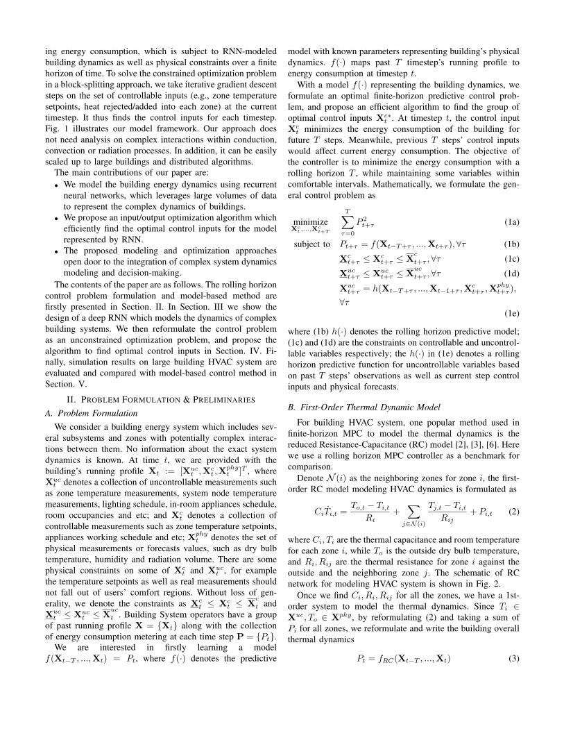
B. First-Order Thermal Dynamic Model

For building HVAC system, one popular method used infinite-horizon MPC to model the thermal dynamics is thereduced Resistance-Capacitance (RC) model [2], [3], [6]. Herewe use a rolling horizon MPC controller as a benchmark forcomparison.

Denote N (i) as the neighboring zones for zone i, the first-order RC model modeling HVAC dynamics is formulated as

CiTi,t =To,t − Ti,t

Ri+

∑j∈N (i)

Tj,t − Ti,tRij

+ Pi,t (2)

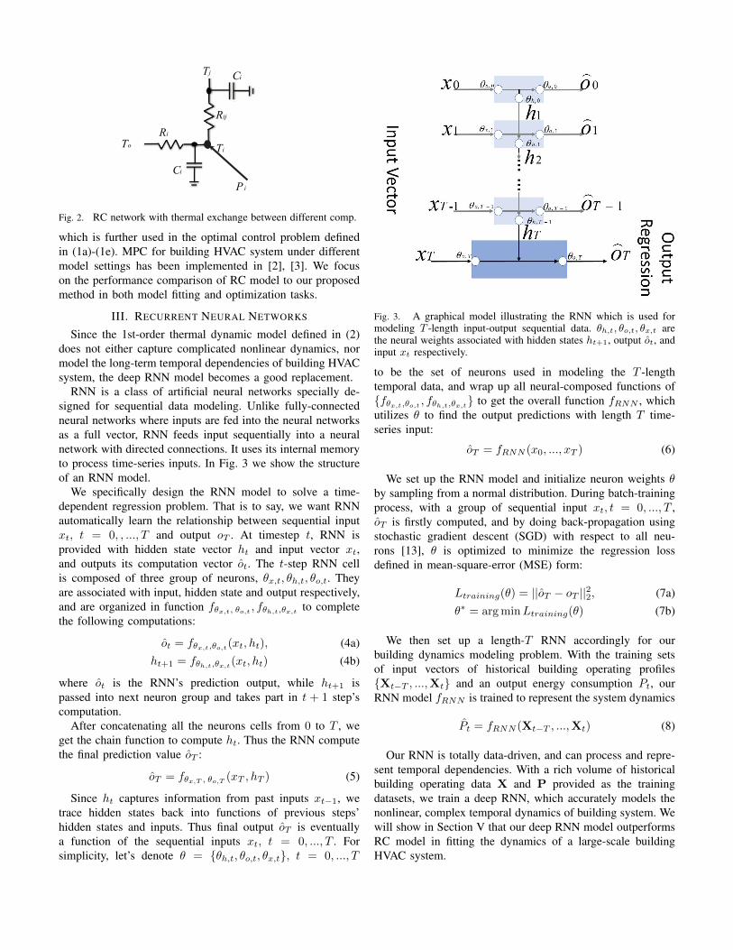
where Ci, Ti are the thermal capacitance and room temperaturefor each zone i, while To is the outside dry bulb temperature,and Ri, Rij are the thermal resistance for zone i against theoutside and the neighboring zone j. The schematic of RCnetwork for modeling HVAC system is shown in Fig. 2.

Once we find Ci, Ri, Rij for all the zones, we have a 1st-order system to model the thermal dynamics. Since Ti ∈Xuc, To ∈ Xphy , by reformulating (2) and taking a sum ofPi for all zones, we reformulate and write the building overallthermal dynamics

Pt = fRC(Xt−T , ...,Xt) (3)

oT

radiationQ

iP

ijR

iC

iR

iC

jT

iT

Fig. 2. RC network with thermal exchange between different comp.

which is further used in the optimal control problem definedin (1a)-(1e). MPC for building HVAC system under differentmodel settings has been implemented in [2], [3]. We focuson the performance comparison of RC model to our proposedmethod in both model fitting and optimization tasks.

III. RECURRENT NEURAL NETWORKS

Since the 1st-order thermal dynamic model defined in (2)does not either capture complicated nonlinear dynamics, normodel the long-term temporal dependencies of building HVACsystem, the deep RNN model becomes a good replacement.

RNN is a class of artificial neural networks specially de-signed for sequential data modeling. Unlike fully-connectedneural networks where inputs are fed into the neural networksas a full vector, RNN feeds input sequentially into a neuralnetwork with directed connections. It uses its internal memoryto process time-series inputs. In Fig. 3 we show the structureof an RNN model.

We specifically design the RNN model to solve a time-dependent regression problem. That is to say, we want RNNautomatically learn the relationship between sequential inputxt, t = 0, , ..., T and output oT . At timestep t, RNN isprovided with hidden state vector ht and input vector xt,and outputs its computation vector ot. The t-step RNN cellis composed of three group of neurons, θx,t, θh,t, θo,t. Theyare associated with input, hidden state and output respectively,and are organized in function fθx,t, θo,t , fθh,t,θx,t to completethe following computations:

ot = fθx,t,θo,t(xt, ht), (4a)ht+1 = fθh,t,θx,t(xt, ht) (4b)

where ot is the RNN’s prediction output, while ht+1 ispassed into next neuron group and takes part in t + 1 step’scomputation.

After concatenating all the neurons cells from 0 to T , weget the chain function to compute ht. Thus the RNN computethe final prediction value oT :

oT = fθx,T , θo,T (xT , hT ) (5)

Since ht captures information from past inputs xt−1, wetrace hidden states back into functions of previous steps’hidden states and inputs. Thus final output oT is eventuallya function of the sequential inputs xt, t = 0, ..., T . Forsimplicity, let’s denote θ = {θh,t, θo,t, θx,t}, t = 0, ..., T

Fig. 3. A graphical model illustrating the RNN which is used formodeling T -length input-output sequential data. θh,t, θo,t, θx,t arethe neural weights associated with hidden states ht+1, output ot, andinput xt respectively.

to be the set of neurons used in modeling the T -lengthtemporal data, and wrap up all neural-composed functions of{fθx,t,θo,t , fθh,t,θx,t} to get the overall function fRNN , whichutilizes θ to find the output predictions with length T time-series input:

oT = fRNN (x0, ..., xT ) (6)

We set up the RNN model and initialize neuron weights θby sampling from a normal distribution. During batch-trainingprocess, with a group of sequential input xt, t = 0, ..., T ,oT is firstly computed, and by doing back-propagation usingstochastic gradient descent (SGD) with respect to all neu-rons [13], θ is optimized to minimize the regression lossdefined in mean-square-error (MSE) form:

Ltraining(θ) = ||oT − oT ||22, (7a)θ∗ = argminLtraining(θ) (7b)

We then set up a length-T RNN accordingly for ourbuilding dynamics modeling problem. With the training setsof input vectors of historical building operating profiles{Xt−T , ...,Xt} and an output energy consumption Pt, ourRNN model fRNN is trained to represent the system dynamics

Pt = fRNN (Xt−T , ...,Xt) (8)

Our RNN is totally data-driven, and can process and repre-sent temporal dependencies. With a rich volume of historicalbuilding operating data X and P provided as the trainingdatasets, we train a deep RNN, which accurately models thenonlinear, complex temporal dynamics of building system. Wewill show in Section V that our deep RNN model outperformsRC model in fitting the dynamics of a large-scale buildingHVAC system.

IV. INPUTS OPTIMIZATION FOR BUILDING CONTROL

In this section we describe our control algorithm which isbased on our pre-trained deep learning model. We demonstratehow it is able to incorporate (8) into the optimization problem(1). We also illustrate how to solve such optimization problemto find a collection of optimal control sequential inputs.

By substituting f(·) in (1) with fRNN , and denote Xvart =

[Xct ,X

uct ],the finite horizon control problem for building en-

ergy management is written as

minimizeXct ,...,X

ct+T

T∑τ=0

P 2t+τ (9a)

subject to Pt+τ = fRNN (Xt−T+τ , ...,Xt+τ ),∀τ (9b)

Xvart+τ ≤ Xvar

t+τ ≤ Xvar

t+τ ,∀τ (9c)

Xuct+τ = h(Xt−T+τ , ...,Xt−1+τ ,X

ct+τ ,X

phyt+τ ),

∀τ(9d)

Since Xuct+τ , τ = 1, ..., T is directly controlled by control in-

puts of previous time. For all the uncontrollable variables withconstraints we model, they also possess pairing controllablevariables, e.g., the temperature measurements-temperature set-points. We then choose Xuc

t+τ = Xct−1+τ , τ = 1, ..., T , since

such uncontrollable values are the control outputs correspond-ing to the previous step’s control inputs. Thus we diminishconstraint (9d).

Since the constrained optimization problem (9) includes anon-convex deep neural network in the constraints, we use logbarriers functions to rewrite the problem in an unconstrainedform:

minXct ,...,X

ct+T

Lopti(Xct , ...,X

ct+T ) =

T∑τ=0

f2RNN (Xt−T+τ , ...,Xt+τ )

− λT∑τ=0

log(Xvart+τ −Xvar

t+τ )

− λT∑τ=0

log(Xvar

t+τ −Xvart+τ )

(10)

where λ is a tuning parameter, and Lopti(Xct , ...,X

ct+T )

defines a loss function with inputs Xct , ...,X

ct+T . We solve

this loss minimization problem by iteratively taking gradientdescents of (10). Note that during RNN model training, weare taking gradients ∇θLtraining(θ) with respect to all theneurons. Once training is done, Ltraining(θ) is converged.The RNN model serves as the temporal physical model, andis always modeling the building system dynamics accurately.Here we are taking gradients with this fixed, pre-trained RNNmodel, and find gradients ∇Xc

t+τLopti(X

ct , ...,X

ct+T ), τ =

0, ..., T with respect to the group of controllable variables.Once Lopti(X

ct , ...,X

ct+T ) is converged, and we find Xc∗

t

that is a local optimal solution. Xc∗

t is also the solution

of controllable inputs for the finite horizon optimal controlproblem at timestep t.

The k-step gradient descent method is working as follows:

gt+τ,k = η∇Xct+τ,kLopti(Xct,k−1, ...,X

ct+T,k−1) (11a)

Xct+τ,k = Xc

t+τ,k−1 − gt+τ,k, τ = 0, ..., T (11b)

where η is the learning rate, and Xct+τ,k denotes the value for

Xct+τ after k step’s update.Throughout our modeling and optimization approach, we do

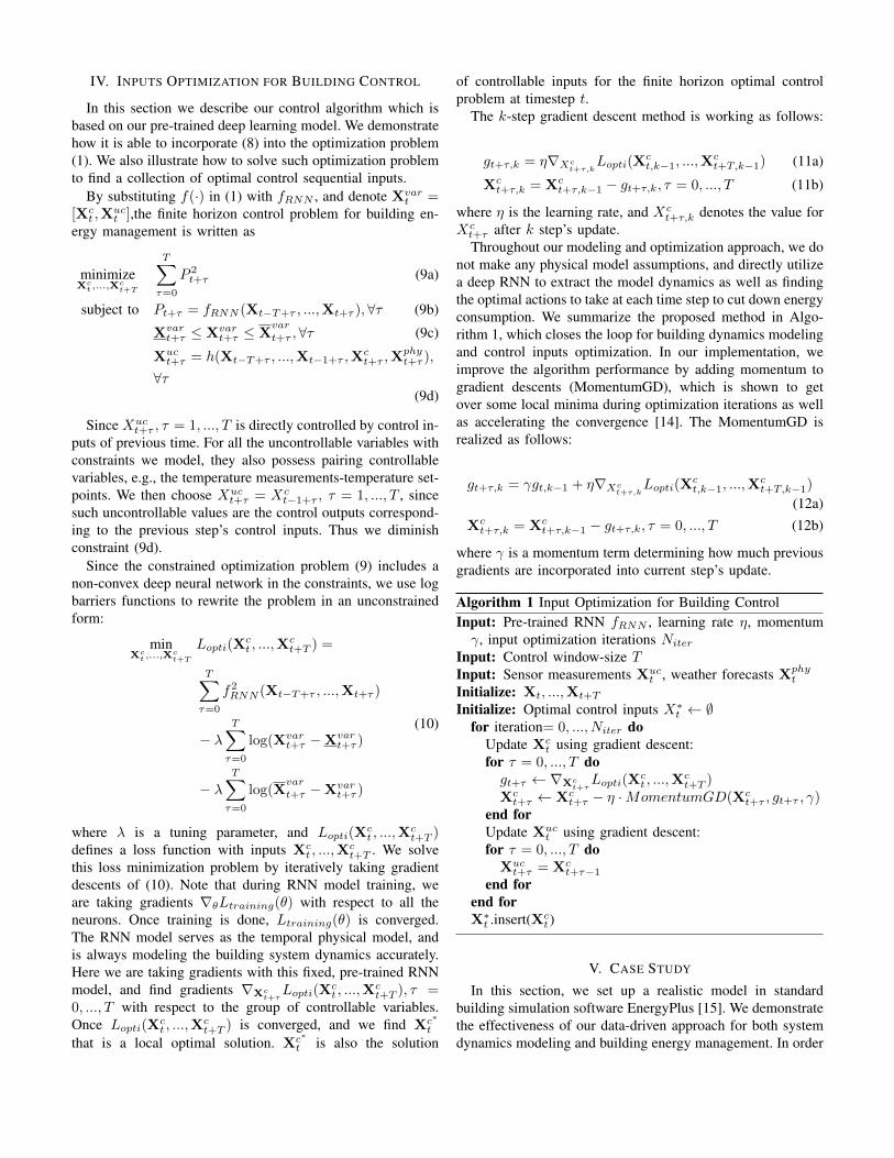
not make any physical model assumptions, and directly utilizea deep RNN to extract the model dynamics as well as findingthe optimal actions to take at each time step to cut down energyconsumption. We summarize the proposed method in Algo-rithm 1, which closes the loop for building dynamics modelingand control inputs optimization. In our implementation, weimprove the algorithm performance by adding momentum togradient descents (MomentumGD), which is shown to getover some local minima during optimization iterations as wellas accelerating the convergence [14]. The MomentumGD isrealized as follows:

gt+τ,k = γgt,k−1 + η∇Xct+τ,kLopti(Xct,k−1, ...,X

ct+T,k−1)

(12a)Xct+τ,k = Xc

t+τ,k−1 − gt+τ,k, τ = 0, ..., T (12b)

where γ is a momentum term determining how much previousgradients are incorporated into current step’s update.

Algorithm 1 Input Optimization for Building ControlInput: Pre-trained RNN fRNN , learning rate η, momentumγ, input optimization iterations Niter

Input: Control window-size TInput: Sensor measurements Xuc

t , weather forecasts Xphyt

Initialize: Xt, ...,Xt+T

Initialize: Optimal control inputs X∗t ← ∅for iteration= 0, ..., Niter do

Update Xct using gradient descent:

for τ = 0, ..., T dogt+τ ← ∇Xc

t+τLopti(X

ct , ...,X

ct+T )

Xct+τ ← Xc

t+τ − η ·MomentumGD(Xct+τ , gt+τ , γ)

end forUpdate Xuc

t using gradient descent:for τ = 0, ..., T doXuct+τ = Xc

t+τ−1end for

end forX∗t .insert(Xc

t )

V. CASE STUDY

In this section, we set up a realistic model in standardbuilding simulation software EnergyPlus [15]. We demonstratethe effectiveness of our data-driven approach for both systemdynamics modeling and building energy management. In order

to compare with the model-based approach, we focus on theHVAC system for a large building complex. But our methodis a general regression and optimization approach, whichcould be easily applied to overall building energy managementproblem.

A. Experimental Setup

We set up our EnergyPlus simulations using a 12-storeylarge office building (in Fig. 4) listed in the commercialreference buildings from U.S. Department of Energy (DoECRB) [16]. The building has a total floor area of 498, 584square feet which is divided into 16 separate zones. Wesimulate the building running through the year of 2004 inSeattle, WA, and record (Xt, Pt) with a resolution of 10minutes. We shuffle and separate 2 months’ data as ourstand-alone testing dataset for both regression and controlperformance evaluation, while the remaining 10 months’ datais used to for RNN training. The processed datasets have 55input features, which include controllable variables such aszone temperature setpoints, and uncontrollable variables suchas zone occupancies and temperature measurements. Outputis a single feature for energy consumption at each timestep.We directly use historical weather data records into both RCmodel and RNN model. For future work, the forecasts modelshould also be considered into the pipeline. A finite horizonof 4 hours is set for both MPC method and proposed method.

We set up our deep learning model using Tensorflow, aPython open-source package. Our RNN model is composed of1 recurrent layer with 3 subsequent fully-connected layers. Weadopt rectified linear unit (ReLU) activation functions, dropoutlayers and Stochastic Gradient Descent (SGD) optimizer toimprove our neural network training.

Fig. 4. Schematic diagram of simulated large commercial building.

B. Simulation Results

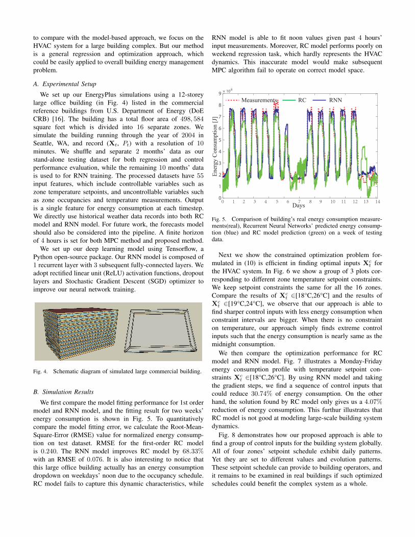
We first compare the model fitting performance for 1st ordermodel and RNN model, and the fitting result for two weeks’energy consumption is shown in Fig. 5. To quantitativelycompare the model fitting error, we calculate the Root-Mean-Square-Error (RMSE) value for normalized energy consump-tion on test dataset. RMSE for the first-order RC modelis 0.240. The RNN model improves RC model by 68.33%with an RMSE of 0.076. It is also interesting to notice thatthis large office building actually has an energy consumptiondropdown on weekdays’ noon due to the occupancy schedule.RC model fails to capture this dynamic characteristics, while

RNN model is able to fit noon values given past 4 hours’input measurements. Moreover, RC model performs poorly onweekend regression task, which hardly represents the HVACdynamics. This inaccurate model would make subsequentMPC algorithm fail to operate on correct model space.

0

1

2

3

4

5

6

7

8

9 × 108

0 1471 2 3 4 5 6 8 9 10 11 12 13Days

Ener

gy C

onsu

mpt

ion

[J]

Measurements RC RNN

Fig. 5. Comparison of building’s real energy consumption measure-ments(real), Recurrent Neural Networks’ predicted energy consump-tion (blue) and RC model prediction (green) on a week of testingdata.

Next we show the constrained optimization problem for-mulated in (10) is efficient in finding optimal inputs Xc

t forthe HVAC system. In Fig. 6 we show a group of 3 plots cor-responding to different zone temperature setpoint constraints.We keep setpoint constraints the same for all the 16 zones.Compare the results of Xc

t ∈[18°C,26°C] and the results ofXct ∈[19°C,24°C], we observe that our approach is able to

find sharper control inputs with less energy consumption whenconstraint intervals are bigger. When there is no constrainton temperature, our approach simply finds extreme controlinputs such that the energy consumption is nearly same as themidnight consumption.

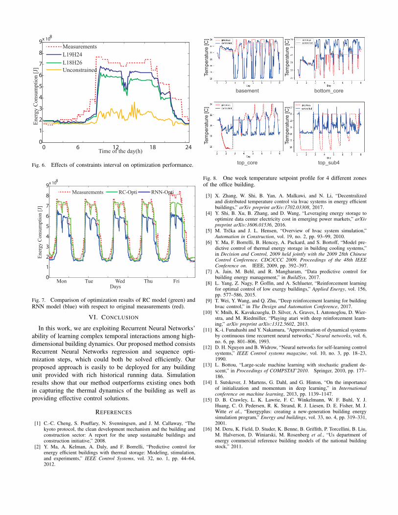
We then compare the optimization performance for RCmodel and RNN model. Fig. 7 illustrates a Monday-Fridayenergy consumption profile with temperature setpoint con-straints Xc

t ∈[18°C,26°C]. By using RNN model and takingthe gradient steps, we find a sequence of control inputs thatcould reduce 30.74% of energy consumption. On the otherhand, the solution found by RC model only gives us a 4.07%reduction of energy consumption. This furthur illustrates thatRC model is not good at modeling large-scale building systemdynamics.

Fig. 8 demonstrates how our proposed approach is able tofind a group of control inputs for the building system globally.All of four zones’ setpoint schedule exhibit daily patterns.Yet they are set to different values and evolution patterns.These setpoint schedule can provide to building operators, andit remains to be examined in real buildings if such optimizedschedules could benefit the complex system as a whole.

0

1

2

3

4

5

6

7

8

9x 108

Time of the day(h)0 24126 18

Measurements

UnconstrainedL18H26L19H24

Ener

gy C

onsu

mpt

ion

[J]

Fig. 6. Effects of constraints interval on optimization performance.

0

1

2

3

4

5

6

7

8

9x 108

Measurements RC-Opti RNN-Opti

DaysMon Tue Wed Thu Fri

Ener

gy C

onsu

mpt

ion

[J]

Fig. 7. Comparison of optimization results of RC model (green) andRNN model (blue) with respect to original measurements (red).

VI. CONCLUSION

In this work, we are exploiting Recurrent Neural Networks’ability of learning complex temporal interactions among high-dimensional building dynamics. Our proposed method consistsRecurrent Neural Networks regression and sequence opti-mization steps, which could both be solved efficiently. Ourproposed approach is easily to be deployed for any buildingunit provided with rich historical running data. Simulationresults show that our method outperforms existing ones bothin capturing the thermal dynamics of the building as well asproviding effective control solutions.

REFERENCES

[1] C.-C. Cheng, S. Pouffary, N. Svenningsen, and J. M. Callaway, “Thekyoto protocol, the clean development mechanism and the building andconstruction sector: A report for the unep sustainable buildings andconstruction initiative,” 2008.

[2] Y. Ma, A. Kelman, A. Daly, and F. Borrelli, “Predictive control forenergy efficient buildings with thermal storage: Modeling, stimulation,and experiments,” IEEE Control Systems, vol. 32, no. 1, pp. 44–64,2012.

top_sub4top_core

basement bottom_core

Tem

pera

ture

[C]

Tem

pera

ture

[C]

Tem

pera

ture

[C]

Tem

pera

ture

[C]

Fig. 8. One week temperature setpoint profile for 4 different zonesof the office building.

[3] X. Zhang, W. Shi, B. Yan, A. Malkawi, and N. Li, “Decentralizedand distributed temperature control via hvac systems in energy efficientbuildings,” arXiv preprint arXiv:1702.03308, 2017.

[4] Y. Shi, B. Xu, B. Zhang, and D. Wang, “Leveraging energy storage tooptimize data center electricity cost in emerging power markets,” arXivpreprint arXiv:1606.01536, 2016.

[5] M. Trcka and J. L. Hensen, “Overview of hvac system simulation,”Automation in Construction, vol. 19, no. 2, pp. 93–99, 2010.

[6] Y. Ma, F. Borrelli, B. Hencey, A. Packard, and S. Bortoff, “Model pre-dictive control of thermal energy storage in building cooling systems,”in Decision and Control, 2009 held jointly with the 2009 28th ChineseControl Conference. CDC/CCC 2009. Proceedings of the 48th IEEEConference on. IEEE, 2009, pp. 392–397.

[7] A. Jain, M. Behl, and R. Mangharam, “Data predictive control forbuilding energy management,” in BuildSys, 2017.

[8] L. Yang, Z. Nagy, P. Goffin, and A. Schlueter, “Reinforcement learningfor optimal control of low exergy buildings,” Applied Energy, vol. 156,pp. 577–586, 2015.

[9] T. Wei, Y. Wang, and Q. Zhu, “Deep reinforcement learning for buildinghvac control,” in The Design and Automation Conference, 2017.

[10] V. Mnih, K. Kavukcuoglu, D. Silver, A. Graves, I. Antonoglou, D. Wier-stra, and M. Riedmiller, “Playing atari with deep reinforcement learn-ing,” arXiv preprint arXiv:1312.5602, 2013.

[11] K.-i. Funahashi and Y. Nakamura, “Approximation of dynamical systemsby continuous time recurrent neural networks,” Neural networks, vol. 6,no. 6, pp. 801–806, 1993.

[12] D. H. Nguyen and B. Widrow, “Neural networks for self-learning controlsystems,” IEEE Control systems magazine, vol. 10, no. 3, pp. 18–23,1990.

[13] L. Bottou, “Large-scale machine learning with stochastic gradient de-scent,” in Proceedings of COMPSTAT’2010. Springer, 2010, pp. 177–186.

[14] I. Sutskever, J. Martens, G. Dahl, and G. Hinton, “On the importanceof initialization and momentum in deep learning,” in Internationalconference on machine learning, 2013, pp. 1139–1147.

[15] D. B. Crawley, L. K. Lawrie, F. C. Winkelmann, W. F. Buhl, Y. J.Huang, C. O. Pedersen, R. K. Strand, R. J. Liesen, D. E. Fisher, M. J.Witte et al., “Energyplus: creating a new-generation building energysimulation program,” Energy and buildings, vol. 33, no. 4, pp. 319–331,2001.

[16] M. Deru, K. Field, D. Studer, K. Benne, B. Griffith, P. Torcellini, B. Liu,M. Halverson, D. Winiarski, M. Rosenberg et al., “Us department ofenergy commercial reference building models of the national buildingstock,” 2011.