Modeling coating flaws with non-linearpolarization curves for long pipelines

Douglas P. Riemer,1 Mark E. Orazem21 OLI Systems, Inc., USA2 Department of Chemical Engineering, University of Florida, USA

Abstract

External corrosion is commonly mitigated by coating the structure with a highresistance film and by employing cathodic protection (CP) to protect regions thatare inadequately coated or where the coating has degraded. Defects in the coatingare termed holidays, and such holidays can expose bare steel. The objective of thispaper is to explore the state-of-the-art in computer models for cathodic protection.The emphasis is placed here on mitigation of corrosion of underground pipelines,but the concepts, models, and techniques described are sufficiently general to beapplied to mitigation of corrosion of any structure.

1 Introduction

Since the beginning of the 20th century, petroleum products and natural gas havebeen transported over long distances by buried steel pipelines. Over 1.3 millionmiles of buried steel main-line pipe are used to transport natural gas within theUnited States [1]. An additional 170,000 miles of pipeline are used to transportcrude oil and refined petroleum products [2].

The limited availability of right-of-way corridors requires that new pipelines belocated next to existing pipelines. Placement of pipelines in close proximity intro-duces the potential for interference between systems providing cathodic protectionto the respective pipelines. In addition, the modern use of coatings, introduced tolower the current requirement for cathodic protection of pipelines, introduces aswell the potential for localized failure of pipes at discrete coating defects. The pre-diction of the performance of cathodic protection systems under these conditionsrequires a mathematical model that can account for current and potential distribu-tions in both angular and axial directions.

The objective of this work is to describe a mathematical model that has beendeveloped for cathodic protection of a arbitrary number of pipelines linked to anarbitrary number of cathodic protection systems. The Boundary Element Methodwas used in the model formulation. In order to achieve the desired calculationaccuracy and speed, the development required significant refinement to algorithmsavailable in the literature.

2 Mathematical development

The model for cathodic protection of pipelines must account for the flow of cur-rent in the soil, in the pipes, and in the circuitry. Until recently, most models ofcathodic protection of pipelines assumed that the potential of the pipe steel wasuniform. The assumption of a uniform steel potential enabled solution for currentand potential distributions without consideration of the passage of current throughthe pipe. Long pipes, however, exhibit a non-negligible potential difference alongthe steel [3, 4, 5].

In the context of the present work, there exist two separate domains for theflow of current. The first is the soil (or outer) domain, bounded by the surfacesof the pipes and anodes, the interface between the soil and air, and, if present,the interface between the soil and any buried insulating layers. The second (inner)domain comprises the metallic wall of the pipe, the volume of the anode, andconnecting wires and resistors for the return path of the protective current. Thetwo domains are linked by the electrochemical reactions described in section 2.3.

2.1 Soil (or outer) domain

The soil domain comprises the material in which the pipes and anodes are buried.From the perspective of the pipe, this domain can be considered to be an outerdomain. This designation contrasts the soil domain from the domain which includesthe interior volume of pipeline steel.

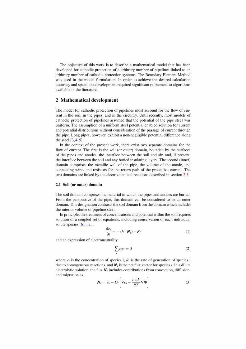
In principle, the treatment of concentrations and potential within the soil requiressolution of a coupled set of equations, including conservation of each individualsolute species [6], i.e., ,

∂ci

∂t=−(∇ ·NNNi)+Ri (1)

and an expression of electroneutrality

∑i

zici = 0 (2)

where ci is the concentration of species i, Ri is the rate of generation of species idue to homogeneous reactions, and NNNi is the net flux vector for species i. In a diluteelectrolytic solution, the flux NNNi includes contributions from convection, diffusion,and migration as

NNNi = vvvc−Di

[∇ci−

ziciFRT

∇Φ

](3)

where vvv is the fluid velocity, Di is the diffusion coefficient for species i, zi is thecharge associated with species i, F is Faraday’s constant, and Φ is the potential.

Under the assumption of a steady-state and a uniform concentration of ionicspecies, the current density, expressed in terms of contributions from the motionof each ionic species, can be given in terms of potential by Ohm’s law. Thus,

iii = F ∑i

ziNNNi =−κ∇Φ (4)

where the conductivity κ, expressed in terms of contributions from individualspecies as

κ = F2∑

iz2

i uici (5)

has a uniform value because the concentration is uniform. The assumption thatconcentrations are uniform yields

∇2Φ = 0. (6)

Thus, potential is governed by Laplace’s equation.Equation (6) is commonly used without explanation in cathodic protection mod-

els. The development presented above can be used to emphasize some importantpoints.

• The assumption that concentrations are uniform means that concentrationgradients associated with reactions on the pipe and anode surface are assumedto occur within a thin layer adjacent to the pipe and anode surfaces. The con-centration gradients within this narrow layer can be incorporated into theboundary condition which describes the electrochemical reactions.

• While changes in soil resistivity can be treated within Boundary Elementmodels by creating coupled soil domains, the variation of potential acrossthe boundaries between domains must include the contribution of a diffusionpotential associated with concentration gradients.

The resistivity of the soil domain was assumed to be uniform in the present model.

2.2 Pipe metal (or inner) domain

The potential drop within the pipeline steel can be very significant when the cur-rent level is large and the pipelines are long. The Ohmic resistance of a ANSI Stan-dard 18-inch (0.457 m) diameter steel pipe with a wall thickness of 0.375 inches(0.95 cm) is 7.2× 10−3 Ω/km. The potential drop along a 100 km length of thispipe would be 720 mV for passage of a relatively modest 1 A of CP current. Theassumption that the potential drop in the pipe steel can be neglected, made, forexample, by Esteban et al [7] for their treatment of coating holidays in a shortlength of pipe, cannot be made for longer stretches of pipeline networks.

The flow of current through the pipe steel, anodes, and connecting wires isstrictly governed by the Laplace’s equation

∇ · (κ∇V ) = 0 (7)

where V is the departure of the potential of the metal from an uniform value andκ is the material conductivity. The conductivity of the pipe-metal domain κ isnot necessarily uniform. For example, the copper wires connecting the pipe tothe anode has a different conductivity than does pipeline steel or the anode orgroundbed material. A simplified version of equation (7)

∆V = IR = IρLA

(8)

can be used to account for the potential drop across connecting wires, where R isthe resistance of the wire, ρ is the electrical resistivity, L is the length, and A is thecross-sectional area of wire.

2.3 Domain coupling through boundary conditions

The inner and outer domains described in sections 2.1 and 2.2, respectively, arelinked by boundary conditions which relate the current density on metal surfacesto values of local potential. The type of surface governs the specific form of therelationship required. Bare steel, coated steel, galvanic anodes, and impressed cur-rent anodes are considered in the following sections.

2.3.1 Bare steelWhile the surface of modern pipelines are generally covered by a protective coat-ing, bare metal can be exposed by coating defects caused by mechanical damageor long-term degradation mechanisms. For steel in soil, the electrochemical reac-tions include corrosion, oxygen reduction, and, at sufficiently cathodic potentials,hydrogen evolution. One common form of the boundary condition, adapted forsteady-state soil systems by Yan et al [8] and Kennelly et al [9], takes the form

i = 10(V−Φ−EFe)/βFe −(

1ilim,O2

−10(V−Φ−EO2 )/βO2

)−1

−10−(V−Φ−EH2 )/βH2 (9)

where V is the potential of the steel, obtained from solution of the inner domain,and Φ is the potential of the soil adjacent to the steel, obtained from solutionof the outer domain. The term βFe represents the Tafel slope for the corrosionreaction, and EFe represents the equilibrium potential for the corrosion reaction.Similar terms are used for the oxygen reduction and hydrogen evolution reactions.The mass transfer of oxygen is taken into account by including the mass transferlimited current density for oxygen reduction ilim,O2 .

The influence of calcareous and corrosion-product films on the bare surfacecan be taken into account by adjusting the kinetic parameter values. Nisancioglu[10, 11, 12] showed how the parameters of polarization curves can be adjusted in

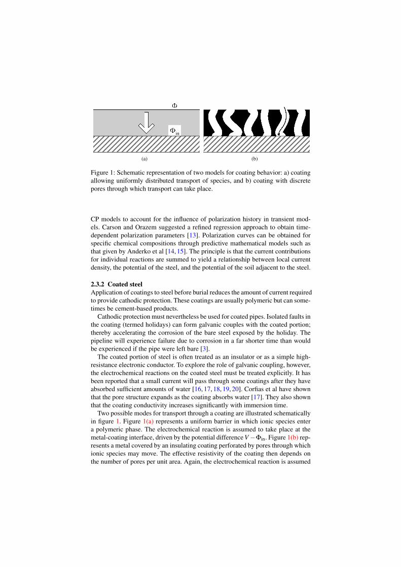
(a) (b)

Figure 1: Schematic representation of two models for coating behavior: a) coatingallowing uniformly distributed transport of species, and b) coating with discretepores through which transport can take place.

CP models to account for the influence of polarization history in transient mod-els. Carson and Orazem suggested a refined regression approach to obtain time-dependent polarization parameters [13]. Polarization curves can be obtained forspecific chemical compositions through predictive mathematical models such asthat given by Anderko et al [14, 15]. The principle is that the current contributionsfor individual reactions are summed to yield a relationship between local currentdensity, the potential of the steel, and the potential of the soil adjacent to the steel.

2.3.2 Coated steelApplication of coatings to steel before burial reduces the amount of current requiredto provide cathodic protection. These coatings are usually polymeric but can some-times be cement-based products.

Cathodic protection must nevertheless be used for coated pipes. Isolated faults inthe coating (termed holidays) can form galvanic couples with the coated portion;thereby accelerating the corrosion of the bare steel exposed by the holiday. Thepipeline will experience failure due to corrosion in a far shorter time than wouldbe experienced if the pipe were left bare [3].

The coated portion of steel is often treated as an insulator or as a simple high-resistance electronic conductor. To explore the role of galvanic coupling, however,the electrochemical reactions on the coated steel must be treated explicitly. It hasbeen reported that a small current will pass through some coatings after they haveabsorbed sufficient amounts of water [16, 17, 18, 19, 20]. Corfias et al have shownthat the pore structure expands as the coating absorbs water [17]. They also shownthat the coating conductivity increases significantly with immersion time.

Two possible modes for transport through a coating are illustrated schematicallyin figure 1. Figure 1(a) represents a uniform barrier in which ionic species entera polymeric phase. The electrochemical reaction is assumed to take place at themetal-coating interface, driven by the potential difference V −Φin. Figure 1(b) rep-resents a metal covered by an insulating coating perforated by pores through whichionic species may move. The effective resistivity of the coating then depends onthe number of pores per unit area. Again, the electrochemical reaction is assumed

to take place at the metal-coating interface and is driven by the potential differenceV −Φin. The view of a coated steel represented in figure 1 is supported by resultsreported by NOVA Gas [21] and CC Technologies [19, 22, 23], which showed thatcoatings on steel pipe formed a diffusion barrier when placed in aqueous environ-ments, that the coating absorbs water, and that it is possible to polarize slightly thesteel under a disbonded coating.

The modification of equation (9) by Riemer and Orazem [24, 25] can addresseither mode of transport illustrated in figure 1. The potential drop through the filmor coating can be expressed as [7]

i =Φ−Φin

ρδ(10)

where Φ is the potential in the electrolyte next to the coating, Φin is the potentialat the underside of the coating just above the steel, ρ is the effective resistivity ofthe coating and δ is the thickness of the coating. The current density can also bewritten in terms of the electrochemical reactions as

i =Apore

A

[10(V−Φin−EFe)/βFe −

(1

(1−αblk) ilim,O2

−10(V−Φin−EO2 )/βO2

)−1

−10−(V−Φin−EH2)/βH2

] (11)

where Apore/A is the effective surface area available for reactions, and αblk is thereduction to the transport of oxygen through the barrier. It is also assumed thatthe coating has absorbed enough water that the hydrogen evolution reaction isnot mass-transfer limited. Equations (10) and (11) are solved simultaneously by aNewton-Ralphson method to get values for the current density and Φin.

By eliminating the current density in equations (10) and (11), a particularlyuseful equation is obtained as

A(Φ−Φin)Aporeρfilmδfilm

= 10(V−Φin−EFe)/βFe

−(

1(1−αblk) ilim,O2

−10(V−Φin−EO2 )/βO2

)−1

−10−(V−Φin−EH2)/βH2

(12)

which links V , Φ, and Φin. Equation (12) can be solved by a Newton-Ralphsonmethod to get Φin for given values of V and Φ. The current density can subse-quently be calculated from equation (10).

The corrosion potential of the coated steel can be calculated from equation (11)under the assumption that no current flows through the coating. If (1−αblk) issmaller than the pore ratio, then the metal will be more active than bare steel. Ifthey are the same, then the coated pipe and bare steel will have the same corrosionpotential. If (1−αblk) is larger than the pore ratio, the metal under the coating will

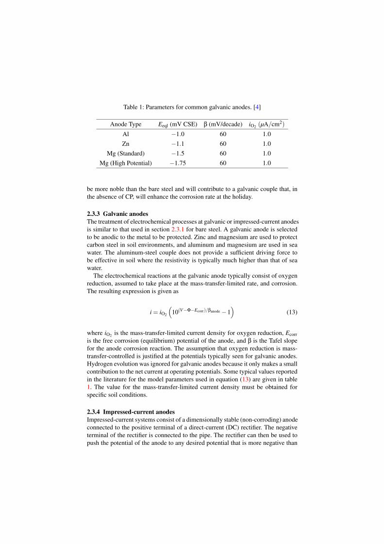
Table 1: Parameters for common galvanic anodes. [4]

Anode Type Eeql (mV CSE) β (mV/decade) iO2 (µA/cm2)

Al −1.0 60 1.0Zn −1.1 60 1.0

Mg (Standard) −1.5 60 1.0Mg (High Potential) −1.75 60 1.0

be more noble than the bare steel and will contribute to a galvanic couple that, inthe absence of CP, will enhance the corrosion rate at the holiday.

2.3.3 Galvanic anodesThe treatment of electrochemical processes at galvanic or impressed-current anodesis similar to that used in section 2.3.1 for bare steel. A galvanic anode is selectedto be anodic to the metal to be protected. Zinc and magnesium are used to protectcarbon steel in soil environments, and aluminum and magnesium are used in seawater. The aluminum-steel couple does not provide a sufficient driving force tobe effective in soil where the resistivity is typically much higher than that of seawater.

The electrochemical reactions at the galvanic anode typically consist of oxygenreduction, assumed to take place at the mass-transfer-limited rate, and corrosion.The resulting expression is given as

i = iO2

(10(V−Φ−Ecorr)/βanode −1

)(13)

where iO2 is the mass-transfer-limited current density for oxygen reduction, Ecorris the free corrosion (equilibrium) potential of the anode, and β is the Tafel slopefor the anode corrosion reaction. The assumption that oxygen reduction is mass-transfer-controlled is justified at the potentials typically seen for galvanic anodes.Hydrogen evolution was ignored for galvanic anodes because it only makes a smallcontribution to the net current at operating potentials. Some typical values reportedin the literature for the model parameters used in equation (13) are given in table1. The value for the mass-transfer-limited current density must be obtained forspecific soil conditions.

2.3.4 Impressed-current anodesImpressed-current systems consist of a dimensionally stable (non-corroding) anodeconnected to the positive terminal of a direct-current (DC) rectifier. The negativeterminal of the rectifier is connected to the pipe. The rectifier can then be used topush the potential of the anode to any desired potential that is more negative than

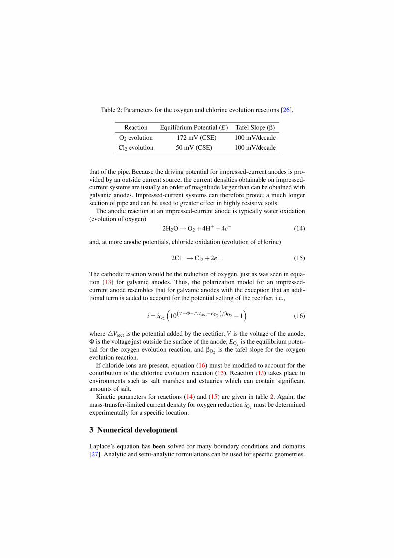
Table 2: Parameters for the oxygen and chlorine evolution reactions [26].

Reaction Equilibrium Potential (E) Tafel Slope (β)

O2 evolution −172 mV (CSE) 100 mV/decadeCl2 evolution 50 mV (CSE) 100 mV/decade

that of the pipe. Because the driving potential for impressed-current anodes is pro-vided by an outside current source, the current densities obtainable on impressed-current systems are usually an order of magnitude larger than can be obtained withgalvanic anodes. Impressed-current systems can therefore protect a much longersection of pipe and can be used to greater effect in highly resistive soils.

The anodic reaction at an impressed-current anode is typically water oxidation(evolution of oxygen)

2H2O → O2 +4H+ +4e− (14)

and, at more anodic potentials, chloride oxidation (evolution of chlorine)

2Cl− → Cl2 +2e−. (15)

The cathodic reaction would be the reduction of oxygen, just as was seen in equa-tion (13) for galvanic anodes. Thus, the polarization model for an impressed-current anode resembles that for galvanic anodes with the exception that an addi-tional term is added to account for the potential setting of the rectifier, i.e.,

i = iO2

(10(V−Φ−4Vrect−EO2)/βO2 −1

)(16)

where 4Vrect is the potential added by the rectifier, V is the voltage of the anode,Φ is the voltage just outside the surface of the anode, EO2 is the equilibrium poten-tial for the oxygen evolution reaction, and βO2 is the tafel slope for the oxygenevolution reaction.

If chloride ions are present, equation (16) must be modified to account for thecontribution of the chlorine evolution reaction (15). Reaction (15) takes place inenvironments such as salt marshes and estuaries which can contain significantamounts of salt.

Kinetic parameters for reactions (14) and (15) are given in table 2. Again, themass-transfer-limited current density for oxygen reduction iO2 must be determinedexperimentally for a specific location.

3 Numerical development

Laplace’s equation has been solved for many boundary conditions and domains[27]. Analytic and semi-analytic formulations can be used for specific geometries.

For example, Moulton first applied the Schwartz-Christoffel transformation to cal-culate analytically the conduction of current through a two-dimensional rectangu-lar geometry with arbitrarily placed electrodes [28]. Bowman supplies details foranalytic solutions using the Schwartz-Christoffel transformation [29]. Orazem andNewman provide a semi-analytical implementation of the Schwartz-Christoffeltransformation for the more complicated structure of a slotted electrode [30]. Orazemused the technique for a compact tension fracture specimen [31] which was laterfurther refined [32]. Diem et al take the semi-analytical technique a step further byallowing for insulating surfaces to form an arbitrary angle with the electrode [33].

Unfortunately, such analytic and semi-analytic approaches are not sufficientlygeneral to allow all the possible configurations of pipes within a domain, thedetailed treatment of potential variation within the pipes, and the polarizationbehavior of the metal surfaces. Thus, numerical techniques are required. Of theavailable techniques, the boundary element method is particularly attractive becauseit can provide accurate calculations for arbitrary geometry. The method only solvesthe governing equation on the boundaries, which is ideal for corrosion problemswhere all the activity takes place at the boundaries. Brebbia first applied the bound-ary element method for potential problems governed by Laplace’s equation [34].Aoki [35] and Telles [36] reported the first practical utilization of the boundaryelement method with simple nonlinear boundary conditions. Zamani and Chuangdemonstrated optimization of cathodic current through adjustment of anode lo-cation [37].

The pipe steel domain is solved using the finite element method. Brichau firstdemonstrated the technique of coupling a finite element solution for pipe steel toa boundary element solution for the soil [38]. He also demonstrated stray cur-rent effects from electric railroad interference utilizing the same solution form-ulation [39]. However, Brichau’s method was limited in that it assumed that thepotential and current distributions on the pipes and anodes were axisymmetricallowing only axial variations. Aoki presented a technique similar to Brichau’s thatincluded optimization of anode locations and several soil conductivity changes forthe case of a single pipe with no angular variations in potential and current distri-butions [40, 41].

Since it is desired to have a solution for the current and potential distributionsboth around the circumference and along the length of the pipe, Brichau’s methodmust be modified. These modifications are described in the following sections.The elements of the BEM and FEM techniques which are well established in theliterature are summarized here for completeness.

3.1 Outer domain: boundary element method

The boundary element method can be derived from the same technique used toobtain the classical finite element method. One starts by writing a variational orweighted residual of the governing differential equation. If the PDE takes the form

∇2u− f = 0 (17)

where f is a forcing term that is a function of position only, then one would writethe weighted residual as

ZΩ

w(∇

2u− f)

dΩ = 0,∀w (18)

where Ω is the domain and w is any weighting function. In the case of Laplace’sequation, f = 0 and u = Φ; thus

ZΩ

w∇2ΦdΩ = 0,∀w. (19)

This equation holds for all weighting functions w. Equation (19) is integrated ana-lytically by using the divergence theorem

ZΩ

∇w∇ΦdΩ−Z

Γ

w(~n ·∇Φ)dΓ = 0,∀w (20)

with Γ being the boundary of the domain. Equation (20) is the classical weak formof the finite element method for Laplace’s equation. At this stage, the boundaryelement method development departs from the finite element method by usinga second application of the divergence theorem. The highest order derivative isthereby moved to the weighting function, i.e.,

ZΩ

Φ∇2wdΩ−

ZΓ

w(~n ·∇Φ)dΓ+Z

Γ

Φ(~n ·∇w)dΓ = 0,∀w. (21)

At this point the weighting function needs to be specified to show why the secondapplication of the divergence theorem was done. If one observes that the solutionto the equation

∇2Gi, j +δi = 0 (22)

is the Greens function for Laplace’s equation, one can simplify equation (21) bypicking the weighting function to be the Green’s function. [42] The first integralin equation (21) becomes

ZΩ

Φ(−δi)dΩ =−Φi. (23)

Substitution of equation (23) into equation (21) yields a simpler equation validwithin the domain

Φi +Z

Γ

Φ(~n ·∇Gi, j)dΓ =Z

Γ

Gi, j (~n ·∇Φ)dΓ (24)

where the highest order derivative has been removed and all the integrals are alongthe boundaries only. Equation (24) is still exact in so far as the Green’s functionis known and is valid for determining the values of the potential at any interiorpoint in the domain given that the potential and current density distributions on theboundary are known. This implies that, for Laplace’s equation, values of interiorpoints are fully specified by integrals along the boundary only.

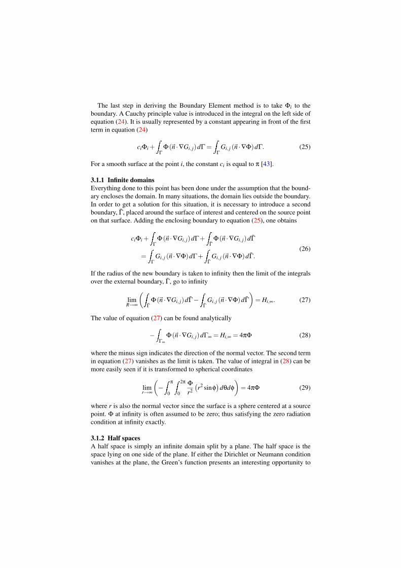
The last step in deriving the Boundary Element method is to take Φi to theboundary. A Cauchy principle value is introduced in the integral on the left side ofequation (24). It is usually represented by a constant appearing in front of the firstterm in equation (24)

ciΦi +Z

Γ

Φ(~n ·∇Gi, j)dΓ =Z

Γ

Gi, j (~n ·∇Φ)dΓ. (25)

For a smooth surface at the point i, the constant ci is equal to π [43].

3.1.1 Infinite domainsEverything done to this point has been done under the assumption that the bound-ary encloses the domain. In many situations, the domain lies outside the boundary.In order to get a solution for this situation, it is necessary to introduce a secondboundary, Γ, placed around the surface of interest and centered on the source pointon that surface. Adding the enclosing boundary to equation (25), one obtains

ciΦi +Z

Γ

Φ(~n ·∇Gi, j)dΓ+Z

Γ

Φ(~n ·∇Gi, j)dΓ

=Z

Γ

Gi, j (~n ·∇Φ)dΓ+Z

Γ

Gi, j (~n ·∇Φ)dΓ.(26)

If the radius of the new boundary is taken to infinity then the limit of the integralsover the external boundary, Γ, go to infinity

limR→∞

(ZΓ

Φ(~n ·∇Gi, j)dΓ−Z

Γ

Gi, j (~n ·∇Φ)dΓ

)= Hi,∞. (27)

The value of equation (27) can be found analytically

−Z

Γ∞

Φ(~n ·∇Gi, j)dΓ∞ = Hi,∞ = 4πΦ (28)

where the minus sign indicates the direction of the normal vector. The second termin equation (27) vanishes as the limit is taken. The value of integral in (28) can bemore easily seen if it is transformed to spherical coordinates

limr→∞

(−Z

π

0

Z 2π

0

Φ

r2

(r2 sinφ

)dθdφ

)= 4πΦ (29)

where r is also the normal vector since the surface is a sphere centered at a sourcepoint. Φ at infinity is often assumed to be zero; thus satisfying the zero radiationcondition at infinity exactly.

3.1.2 Half spacesA half space is simply an infinite domain split by a plane. The half space is thespace lying on one side of the plane. If either the Dirichlet or Neumann conditionvanishes at the plane, the Green’s function presents an interesting opportunity to

satisfy that condition exactly with a very small additional computation when eval-uating the kernels of the integrals. This is done by making use of the reflectionproperties of Green’s functions [43, 44, 45, 46]. In the case of buried pipelines, theNeumann condition vanishes at the plane boundary, i.e., there is no current flowingout of the soil into the air, and none is flowing from the air into the soil.

If one starts with the boundary condition on the plane being zero normal currentand places a source at x and its reflection about the plane at x′ [46],

σ(x)(~n ·∇G(x,ξ))+σ(x′

)(~n ·∇G

(x′,ξ

))= 0 (30)

which implies that the two source intensities σ(x), and σ(x′) are equal and have thesame sign. The sign is the same because the outward normal vectors have oppositesigns for the z component for the reflections. The final form of the Green’s functionis

Gi, j =1

4πr(xi,x j)+

14πr(xi,x′j)

(31)

where x′j is the reflected source point.

3.1.3 LayersLayers are created using the same types of Green’s function reflections as describedabove. The only restriction is that one of the two boundary conditions at the inter-face between the two layers must be equal to zero (i.e., either Φ = 0 or~n ·∇Φ = 0)[46]. In the context of cathodic protection of buried pipelines, the only boundarycondition that has physical meaning is a zero normal current condition since thereis no easy way to have an arbitrary plane within the electrolyte that has a potentialequal to zero. Including a plane with a zero Neumann (natural) condition impliesthat there is one region in which current may flow that is bounded by regions ofzero conductivity whose boundaries are defined by the Green’s function reflec-tions. An example would be an underlying rock layer which has zero conductivity.

The resulting functions can be obtained by using equations of the form of equa-tion (30). The Green’s function in three dimensions would then be of the form

Gi, j =Reflections+1

∑k

14πr(xi,x j,k)

(32)

where the index k > 1 refers to the reflection about some plane k. For k = 1, x j,k isthe field point on the real object. If the soil surface is the only reflection used, theresult is the same as equation (31).

An example of a pipeline in a halfspace with an underlying rock layer is shownin figure 2. Two reflections were used. The first accounts for the zero normal cur-rent at the air-soil interface which is represented by the pipe in the air. The secondreflection accounts for the zero normal current at the rock soil interface and isrepresented by the lower pipe.

The influence of the nonconducting layer on the current delivered to a pipe isseen in figure 3 for a sequence of calculations for which the distance r between the

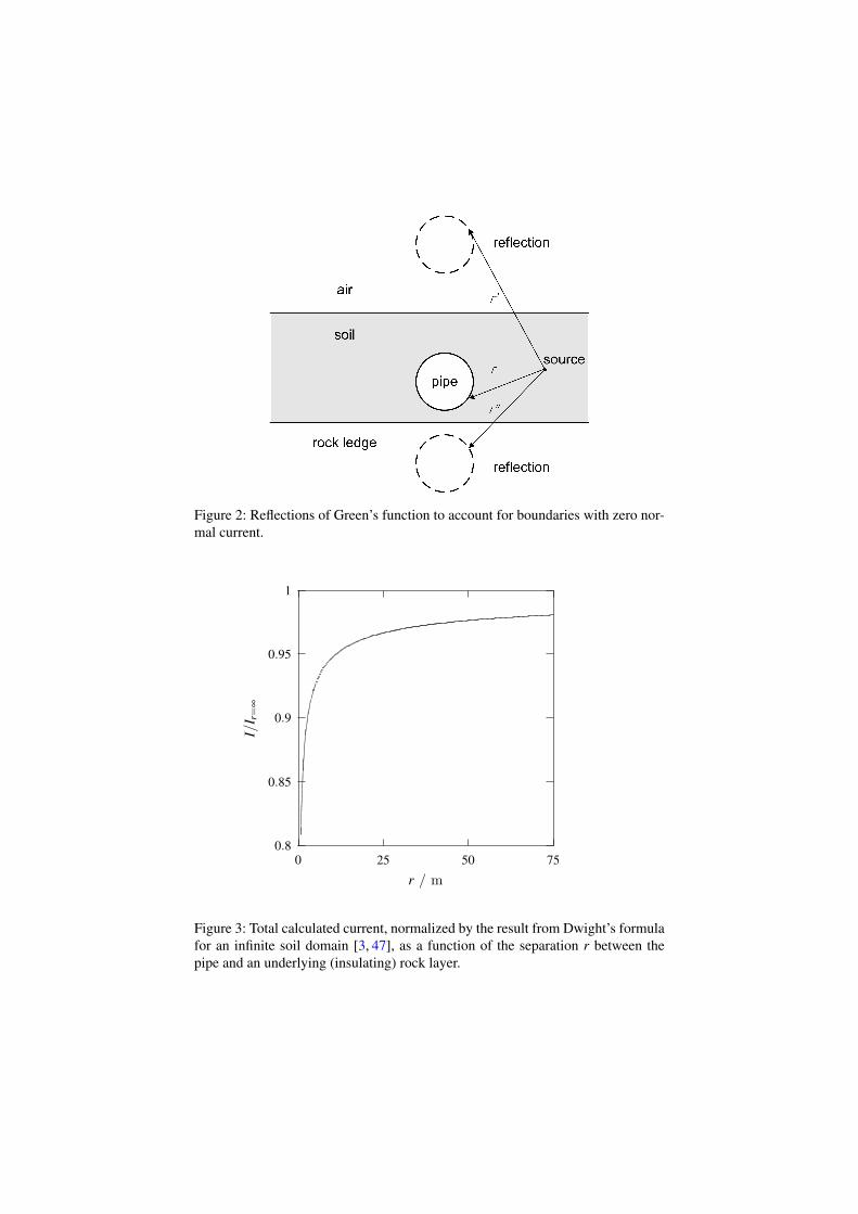
Figure 2: Reflections of Green’s function to account for boundaries with zero nor-mal current.

0.8

0.85

0.9

0.95

1

0 25 50 75

I/I r

=∞

r / m

Figure 3: Total calculated current, normalized by the result from Dwight’s formulafor an infinite soil domain [3, 47], as a function of the separation r between thepipe and an underlying (insulating) rock layer.

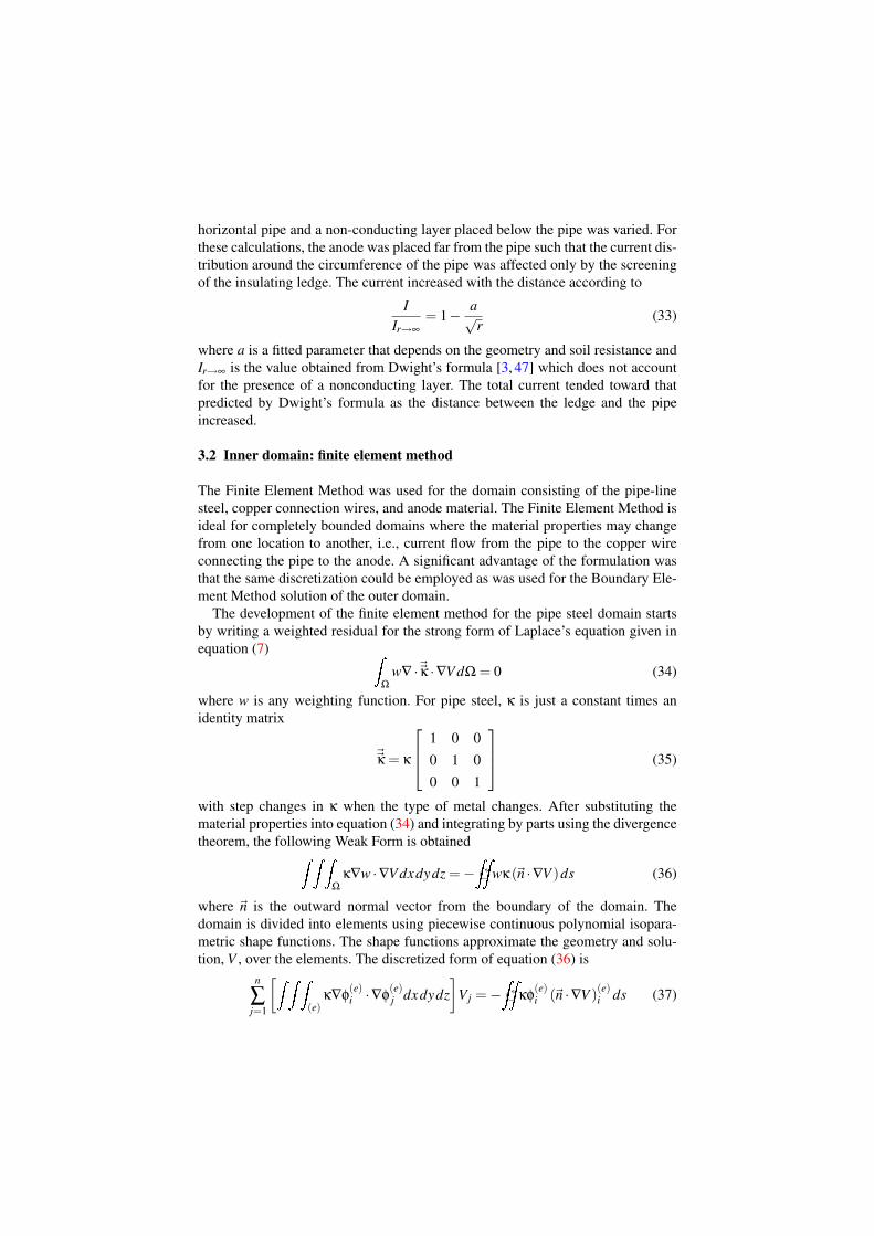
horizontal pipe and a non-conducting layer placed below the pipe was varied. Forthese calculations, the anode was placed far from the pipe such that the current dis-tribution around the circumference of the pipe was affected only by the screeningof the insulating ledge. The current increased with the distance according to

IIr→∞

= 1− a√r

(33)

where a is a fitted parameter that depends on the geometry and soil resistance andIr→∞ is the value obtained from Dwight’s formula [3, 47] which does not accountfor the presence of a nonconducting layer. The total current tended toward thatpredicted by Dwight’s formula as the distance between the ledge and the pipeincreased.

3.2 Inner domain: finite element method

The Finite Element Method was used for the domain consisting of the pipe-linesteel, copper connection wires, and anode material. The Finite Element Method isideal for completely bounded domains where the material properties may changefrom one location to another, i.e., current flow from the pipe to the copper wireconnecting the pipe to the anode. A significant advantage of the formulation wasthat the same discretization could be employed as was used for the Boundary Ele-ment Method solution of the outer domain.

The development of the finite element method for the pipe steel domain startsby writing a weighted residual for the strong form of Laplace’s equation given inequation (7) Z

Ω

w∇ ·~~κ ·∇V dΩ = 0 (34)

where w is any weighting function. For pipe steel, κ is just a constant times anidentity matrix

~~κ = κ

1 0 00 1 00 0 1

(35)

with step changes in κ when the type of metal changes. After substituting thematerial properties into equation (34) and integrating by parts using the divergencetheorem, the following Weak Form is obtainedZ Z Z

Ω

κ∇w ·∇V dxdydz =−ZZwκ(~n ·∇V )ds (36)

where ~n is the outward normal vector from the boundary of the domain. Thedomain is divided into elements using piecewise continuous polynomial isopara-metric shape functions. The shape functions approximate the geometry and solu-tion, V , over the elements. The discretized form of equation (36) is

n

∑j=1

[Z Z Z(e)

κ∇φ(e)i ·∇φ

(e)j dxdydz

]Vj =−

ZZκφ

(e)i (~n ·∇V )(e)i ds (37)

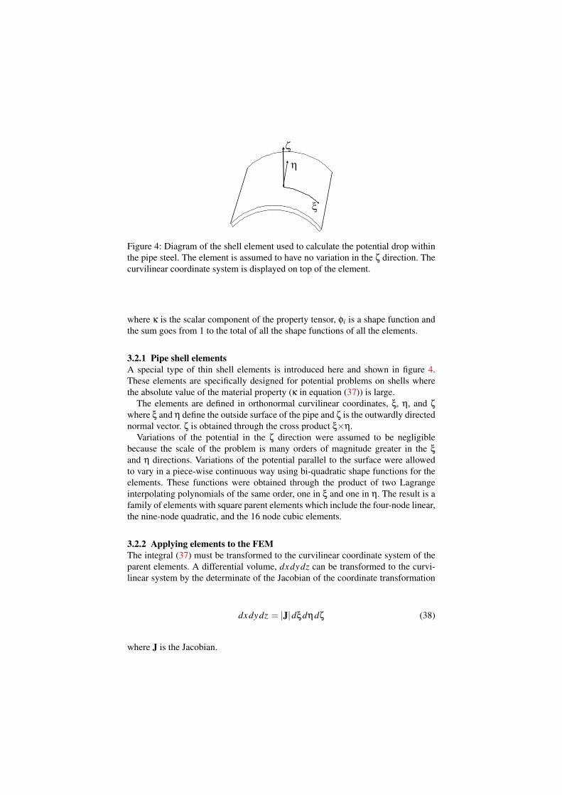
Figure 4: Diagram of the shell element used to calculate the potential drop withinthe pipe steel. The element is assumed to have no variation in the ζ direction. Thecurvilinear coordinate system is displayed on top of the element.

where κ is the scalar component of the property tensor, φi is a shape function andthe sum goes from 1 to the total of all the shape functions of all the elements.

3.2.1 Pipe shell elementsA special type of thin shell elements is introduced here and shown in figure 4.These elements are specifically designed for potential problems on shells wherethe absolute value of the material property (κ in equation (37)) is large.

The elements are defined in orthonormal curvilinear coordinates, ξ, η, and ζ

where ξ and η define the outside surface of the pipe and ζ is the outwardly directednormal vector. ζ is obtained through the cross product ξ×η.

Variations of the potential in the ζ direction were assumed to be negligiblebecause the scale of the problem is many orders of magnitude greater in the ξ

and η directions. Variations of the potential parallel to the surface were allowedto vary in a piece-wise continuous way using bi-quadratic shape functions for theelements. These functions were obtained through the product of two Lagrangeinterpolating polynomials of the same order, one in ξ and one in η. The result is afamily of elements with square parent elements which include the four-node linear,the nine-node quadratic, and the 16 node cubic elements.

3.2.2 Applying elements to the FEMThe integral (37) must be transformed to the curvilinear coordinate system of theparent elements. A differential volume, dxdydz can be transformed to the curvi-linear system by the determinate of the Jacobian of the coordinate transformation

dxdydz = |J|dξdηdζ (38)

where J is the Jacobian.

The Jacobian is composed of the partial derivatives of the coordinates x, y and zwith respect to each of the curvilinear coordinates

J =

∂x∂ξ

∂y∂ξ

∂z∂ξ

∂x∂η

∂y∂η

∂z∂η

∂x∂ζ

∂y∂ζ

∂z∂ζ

. (39)

Integral (37) is transformed to the curvilinear coordinate system to yield

∑i

[Z Z ZΩ(e) ∑

k

∂φi

∂xkκ ·

∂φ j

∂xk|J|dξdηdζ

]=−

ZZ

Γ(e)

wκ(~n ·∇V )ds (40)

where xk is one of the cartesian coordinates, |J| is the determinate of the Jacobian,s is the surface of the element~n is the outward normal vector from the surface, andΩ(e) is the domain of the parent element. The limits of integration in the parentelement are from −1 to +1 for all three of the coordinates. For the special shellelements used for pipes, the integral is only performed numerically over the surfacedξdη which is then scaled by the physical thickness of the shell h, the result ofthe integral over ζ. This requires the Jacobian to be modified to a surface Jacobianwhich, in this case, is simply the square root of the magnitude of the Jacobian.Rewriting equation (40), the two dimensional integral over the surfaces of the pipesis obtained as

∑i

[hZ Z

Ω(e) ∑k

∂φi

∂xkκ ·

∂φ j

∂xk

√|J|dξdη

]=−

ZZ

Γ(e)

wκ(~n ·∇V )ds (41)

with the thickness of the steel, h, a parameter. The normal vector has the samedirection as the one from the boundary element method.

Partial derivatives in equation (41) with respect to cartesian coordinates needto be expressed in terms of the curvilinear coordinates. Using the chain rule, butstarting from the derivatives in cartesian coordinates, one writes

∂φ

∂x∂x∂ξ

+ ∂φ

∂y∂y∂ξ

+ ∂φ

∂z∂z∂ξ

∂φ

∂x∂x∂η

+ ∂φ

∂y∂y∂η

+ ∂φ

∂z∂z∂η

∂φ

∂x∂x∂ζ

+ ∂φ

∂y∂y∂ζ

+ ∂φ

∂z∂z∂ζ

=

∂φ

∂ξ

∂φ

∂η

∂φ

∂ζ

(42)

or, in terms of the Jacobian

J

∂φ

∂x∂φ

∂y∂φ

∂z

=

∂φ

∂ξ

∂φ

∂η

∂φ

∂ζ

. (43)

Since φ is a function of ξ, η, and ζ, the partial derivatives of φ with respect to thecartesian coordinates can be found by inverting the Jacobian.

∂φ

∂x∂φ

∂y∂φ

∂z

= J−1

∂φ

∂ξ

∂φ

∂η

∂φ

∂ζ

. (44)

If J−1i, j is the element from the ith row and the jth column of the inverse of the

Jacobian, then the partial derivatives defined in equation (44) can be expanded toyield

∂φi

∂x= (J−1)11

∂φi

∂ξ+(J−1)12

∂φi

∂η+(J−1)13

∂φi

∂ζ

∂φi

∂y= (J−1)21

∂φi

∂ξ+(J−1)22

∂φi

∂η+(J−1)23

∂φi

∂ζ

∂φi

∂z= (J−1)31

∂φi

∂ξ+(J−1)32

∂φi

∂η+(J−1)33

∂φi

∂ζ.

(45)

The assumption that the thickness of the shell is small with respect to the radiusand length of the shell means that there is negligible variation in the potential inthe ζ direction. Therefore, all terms in equation (45) that involve partial derivativeswith respect to ζ can be assumed to be equal to zero. All of the terms in equation(41) can be evaluated numerically. Since the shape functions for the geometry andsolution vary quadratically in the ξ and η directions, a nine-point Gauss rule (3×3)applied in both directions will give an exact (to machine precision) result.

3.2.3 Bonds and resistorsBonds and resistors are used to provide paths for flow of electrical current betweenpipes or between pipes and anodes. Bonds were implemented as a linear 1D ele-ment between the connection node on one pipe or anode to the connection node onthe second pipe or anode. This formulation requires introduction of no additionalnodes. The material property is set by accounting for the real length and gauge ofthe wire that ties the pipes together. If a resistor is specified within the wire, it isadded to the total resistance of the bond. An illustration of a bond is given in fig-ure 5. The lines connecting the pipes to each other and to the anode are bonds. Thecylinder on the line connecting the two pipes represents a resistor that is sometimesadded in series with the bond to adjust the current load applied to the pipelines.They are modeled as 1D finite elements that connect to the bond connection points.The value of the resistor is set to zero if a resistor is not used in the calculation.

A one-dimensional version of Laplace’s equation is used for the 1D elements.The development for the linear 1D element follows that presented in section 3.2.

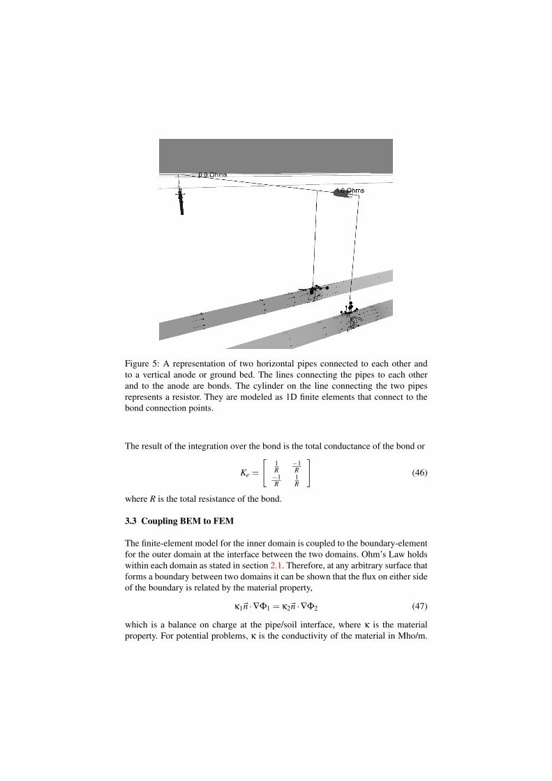
Figure 5: A representation of two horizontal pipes connected to each other andto a vertical anode or ground bed. The lines connecting the pipes to each otherand to the anode are bonds. The cylinder on the line connecting the two pipesrepresents a resistor. They are modeled as 1D finite elements that connect to thebond connection points.

The result of the integration over the bond is the total conductance of the bond or

Ke =

[1R

−1R

−1R

1R

](46)

where R is the total resistance of the bond.

3.3 Coupling BEM to FEM

The finite-element model for the inner domain is coupled to the boundary-elementfor the outer domain at the interface between the two domains. Ohm’s Law holdswithin each domain as stated in section 2.1. Therefore, at any arbitrary surface thatforms a boundary between two domains it can be shown that the flux on either sideof the boundary is related by the material property,

κ1~n ·∇Φ1 = κ2~n ·∇Φ2 (47)

which is a balance on charge at the pipe/soil interface, where κ is the materialproperty. For potential problems, κ is the conductivity of the material in Mho/m.

Using the variables for potential in the pipe, V , and potential in the soil, Φ, theinterface condition is written as

(~n ·∇V ) =κsoil

κsteel(~n ·∇Φ) (48)

where the quantity ~n ·∇V is used in the finite element load integral in equation(41). Equation (48) can be inserted into equation (41) to obtain

∑i

[hZ Z

Ω(e) ∑k

∂φi

∂xkκ ·

∂φ j

∂xk

√|J|dξdη

]=−

ZZ

Γ(e)

wκsoil (~n ·∇Φ)ds. (49)

The right side of equation (49) links the soil domain to the steel domain throughthe current density generated by the kinetics of the corrosion reaction at the steelsurface given by equations (9) and (12).

3.4 Discretization of the boundary elements

Equation (25) may now be applied to a surface that has its boundaries broken upinto individual finite elements. The solution to the differential equation can be rep-resented by approximate functions on each individual element. Example functionsmay be 0th order or constant value, 1st order or linear, etc. The simplest case is theconstant element. The value of Φ is assumed to be constant across each element.Then one can write an equation of the form of (25) for each degree of freedomthat makes up the surface and where the subscript i refers to the element number.The integrals are broken up into N sub-intervals corresponding to N elements thatwhen summed together form the complete integral over the entire boundary

ciφi +∑j

ZΓ j

Φ(~n ·∇Gi, j)dΓ j = ∑j

ZΓ j

Gi, j (~n ·∇Φ)dΓ j. (50)

When constant element are used, the unknown element potentials and normal cur-rent densities can be brought outside the integrals. Since a well-posed problem hasone half of the boundary conditions specified, the result is N equations with Nunknowns.

Since it is desired to be able to change the boundary condition type as well asvalue, the notation used here will denote the matrix resulting from the left handintegral as HHH and the right side as GGG

HHHΦ = GGG(~n ·∇Φ) (51)

where ~n ·∇Φ is the normal current density divided by the conductivity at theboundary.

3.5 Self-Equilibration

Cathodic protection systems are constrained by the requirement that charge is con-served. The boundary element formulation developed in section 2.1 requires modi-fication to satisfy the constraint that charge is conserved. Instead of having a speci-fied potential at infinity (most often set to zero) which serves as a source or sink forcharge, an unknown value of potential at infinity is used such that no current entersor leaves through that boundary. To implement this condition, an extra equation isadded to the system [36, 48]

∑i

ZΓi

κ~n ·∇ΦdΓi = 0. (52)

Equation (52) simply states that all currents entering the boundaries of the domainsum to zero, or, in other words, no current is lost to or gained from infinity. Theleft hand side is added as a new row at the bottom of the GGG matrix of equation(51), while the matrix HHH in (51) receives a row of zeros. A column is added to theHHH matrix which corresponds to the unknown potential at infinity. The values thatare placed in this column come from equation (28) and are all 4π or 1 depend-ing on where the 4π from the Green’s function is placed. This would make the HHHmatrix singular because there is still a row of zeros in it. However, that would onlybe the case if Neumann type boundary conditions are specified everywhere. TheNeumann problem results in an infinite number of solutions that differ by a con-stant. Therefore, at least one element in the system must have a Dirichlet boundarycondition to make the HHH matrix nonsingular and result in a unique solution.

3.6 Multiple CP systems

Riemer and Orazem describe in detail the development needed to model interac-tions among CP systems [25]. To allow stray current between separate CP systems,additional rows can be added of the type introduced in equation (52) [49]. For eachseparate CP system, one extra column in the HHH matrix is also added. The appear-ance of the matrices for 2 CP systems in the same domain will be

GGG =

G1,1 G1,2 G1,3 G1,4

G2,1 G2,2 G2,3 G2,4

0 0 A3 A4

A1 A2 0 0

(53)

HHH =

H1,1 H1,2 0 1H2,1 H2,2 1 0

0 0 0 00 0 0 0

(54)

with the column matrix uuu given by

uuu =

u1

u2

u∞,System2

u∞,System1

(55)

and the column matrix qqq defined in the usual way. When there are two or moreCP systems within a domain, a Dirichlet condition on at least one element in eachCP system must be specified to prevent the HHH matrix from being singular. Theadded equations and unknown potentials at infinity are sufficient to allow severalCP systems to interact with each other while enforcing that the total current oneach CP system sum to zero.

3.7 Nonlinear boundary conditions with attenuation in the pipe steel

The external load integral from the finite-element solution to the inner domain canbe written for each node as a sum of contributions from each element that has thatnode in common

fi =nce

∑`=1

−ZZ

Γ(e)

w`,iκsoil (~n ·∇Φ)ds (56)

where fi is the load for node i and nce is the number of contributing elements to theload at node i. This integral must be evaluated across all nodes on all surfaces ofall structures in the model. Since the value of~n ·∇Φ is either a known or unknownboundary condition from the boundary element method, it must be factored out ofthe integral. Using the shape functions that describe the values of ~n ·∇Φ acrosseach element in terms of the nodal values~n ·∇Φ and the weights, one can rewriteequation (56) as

fi =nce

∑`=1

−ZZ

Γ(e)

w`,iκsoil

nen

∑k=1

φ`,k(s)(~n ·∇Φ)`,k ds (57)

where nen is the number of nodes in the element, (~n ·∇Φ)k is the nodal value of thenormal electric field within the element n, and φ(s)k is the shape function whosevalue is one at node k. Using the property of integrals that an integral of a sum isthe sum of integrals, equation (57) can be rewritten as

fi =nce

∑`=1

nen

∑k=1

−ZZ

Γ(e)

w`,iκsoilφ`,k(s)(~n ·∇Φ)`,k ds. (58)

Equation (58) can then be written in matrix form as

fi =

[. . .−

ZZ

Γ(e)

w`,iκsoilφ`,k(s)ds . . .

](~n ·∇Φ)1,1

...(~n ·∇Φ)ne,nen

(59)

orfi = FFF i [~n ·∇Φ] . (60)

These sub-matrices are then assembled with the right hand column matrix fromequation (51) to form the global finite element system

KKK [V ] = FFF [~n ·∇Φ] (61)

where FFF is a matrix formed from the assembly of equation (60) such that thecolumn matrix corresponding to the Boundary Element Method is formed on theright hand side. FFF is not symmetric.

4 Method for solution of systems of nonlinear equations

The set of variables that appear in the combined soil domain metal domain problemare potentials outside the surface of all pipes or tanks (Φ), unknown normal electricfield on anodes (~n ·∇Φ), and unknown potential difference (V −Φ) for coated andbare protected structures. Introduction of the attenuation code from equation (61)to the problem introduces n more equations and n more unknowns where n is thenumber of nodes used to describe the boundary mesh for the problem. The totalnumber of algebraic equations to be solved is now 2n + k, where k is the numberof separate CP systems.

4.1 Global matrix

The coefficients obtained from the coupled methods are placed into a global matrixsystem and one instance of equation (52) is added for self-equilibriation of eachCP system

HHHc,c HHHa,c 0 0 −4π

HHHc,a HHHa,a 0 0 −4π

0 0 KKKc 0 00 0 0 KKKa 00 0 0 0 0

Φc

Φa

Vp

Va

Φ∞

=

GGGc,c GGGa,c

GGGc,a GGGa,a

FFFc 00 FFFa

Ac Aa

[

~n ·∇Φc

~n ·∇Φa

](62)

where the subscripts a and c refer to anodes and cathodes (pipes) respectively,double subscripts are from the boundary element method and refer to where thesource point and field point lie respectively, and A is the area of each section.

The columns of equation (62) are sorted such that all of the unknown variablesare on the left hand side. For anodes, the unknown variable is the current density(~n ·∇Φ), and for all other structures it is the potential (Φ). The reordered systemthen looks like

HHHc,c −GGGa,c 0 0 −4π

HHHc,a −GGGa,a 0 0 −4π

0 0 KKKc 0 00 −FFFa 0 KKKa 00 −Aa 0 0 0

Φc

~n ·∇Φa

Vc

Va

Φ∞

=

GGGc,c −HHHa,c

GGGc,a −HHHa,a

FFFc 00 0Ac 0

[

~n ·∇Φc

Φa

](63)

where the column matrix on the left hand side is the set of unknown variablesand the column matrix on the right side is the set of known boundary conditions.Equation (63) can be rewritten as

[AAA]

Φc

~n ·∇Φa

Vc

Va

Φ∞

= [BBB]

[~n ·∇Φc

Φa

](64)

where AAA and BBB correspond to the matrices in equation (63).If the boundary conditions are constant, the unknown variables can be obtained

by a simple matrix inversion. For problems in electrochemistry, the set of knownboundary conditions are given as a set of nonlinear functions of the unknown vari-ables. Therefore, the solution must be obtained using a technique for coupled setsof nonlinear algebraic equations. This is done by rewriting equation (64) as a func-tion that is equal to zero

[AAA]

Φc

~n ·∇Φa

Vc

Va

Φ∞

− [BBB]

[~n ·∇Φc = f (V,Φc)Φa = f (V,~n ·∇Φa)

]=

00000

. (65)

Since one of the column matrices contains unknown variables, a guess for thevalues must be made. Since the guess will not be the correct solution to equation

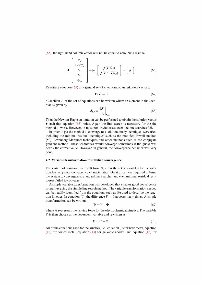
(65), the right hand column vector will not be equal to zero, but a residual

[AAA]

Φc

~n ·∇Φa

Vc

Va

Φ∞

− [BBB]

[f (V,Φc)

f (V,~n ·∇Φa)

]=

[R

]. (66)

Rewriting equation (65) as a general set of equations of an unknown vector xxx

FFF(xxx) = 000 (67)

a Jacobian JJJ, of the set of equations can be written where an element in the Jaco-bian is given by

JJJi, j =∂FFF i

∂xxx j

∣∣∣∣xxx 6= j

. (68)

Then the Newton-Raphson iteration can be performed to obtain the solution vectorxxx such that equation (67) holds. Again the line search is necessary for the themethod to work. However, in most non-trivial cases, even the line searches fail.

In order to get the method to converge to a solution, many techniques were triedincluding the minimal residual techniques such as the modified Powell method[50], Levenberg-Marquort techniques and other methods such as the conjugategradient method. These techniques would converge sometimes if the guess wasnearly the correct value. However, in general, the convergence behavior was verypoor.

4.2 Variable transformation to stabilize convergence

The system of equation that result from Φ,V, i as the set of variables for the solu-tion has very poor convergence characteristics. Great effort was required to bringthe system to convergence. Standard line searches and even minimal residual tech-niques failed to converge.

A simple variable transformation was developed that enables good convergenceproperties using the simple line search method. The variable transformation neededcan be readily identified from the equations such as (9) used to describe the reac-tion kinetics. In equation (9), the difference V −Φ appears many times. A simpletransformation can be written

Ψ = V −Φ (69)

where Ψ represents the driving force for the electrochemical kinetics. The variableV is then chosen as the dependent variable and rewritten as

V = Ψ+Φ. (70)

All of the equations used for the kinetics, i.e., equation (9) for bare metal, equation(12) for coated metal, equation (13) for galvanic anodes, and equation (16) for

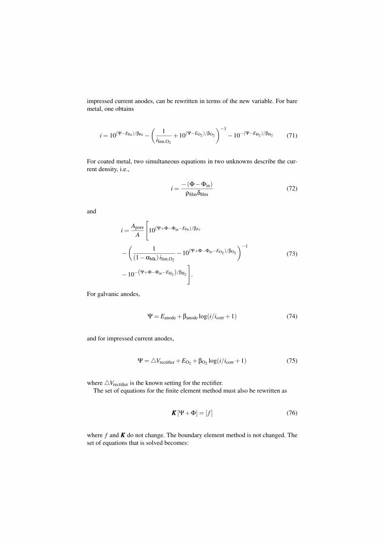
impressed current anodes, can be rewritten in terms of the new variable. For baremetal, one obtains

i = 10(Ψ−EFe)/βFe −(

1ilim,O2

+10(Ψ−EO2 )/βO2

)−1

−10−(Ψ−EH2 )/βH2 (71)

For coated metal, two simultaneous equations in two unknowns describe the cur-rent density, i.e.,

i =−(Φ−Φin)

ρfilmδfilm(72)

and

i =Apore

A

[10(Ψ+Φ−Φin−EFe)/βFe

−(

1(1−αblk) ilim,O2

−10(Ψ+Φ−Φin−EO2 )/βO2

)−1

−10−(Ψ+Φ−Φin−EH2)/βH2

].

(73)

For galvanic anodes,

Ψ = Eanode +βanode log(i/icorr +1) (74)

and for impressed current anodes,

Ψ =4Vrectifier +EO2 +βO2 log(i/icorr +1) (75)

where 4Vrectifier is the known setting for the rectifier.The set of equations for the finite element method must also be rewritten as

KKK [Ψ+Φ] = [ f ] (76)

where f and KKK do not change. The boundary element method is not changed. Theset of equations that is solved becomes:

0 0 HHHc,c HHHa,c −4π

0 0 HHHc,a HHHa,a −4π

KKKc 0 KKKc 0 00 KKKa 0 KKKa 00 0 0 0 0

Ψc

Ψa

Φc

Φa

Φ∞

=

GGGc,c GGGa,c

GGGc,a GGGa,a

FFFc 00 FFFa

Ac Aa

[

~n ·∇Φc

~n ·∇Φa

].

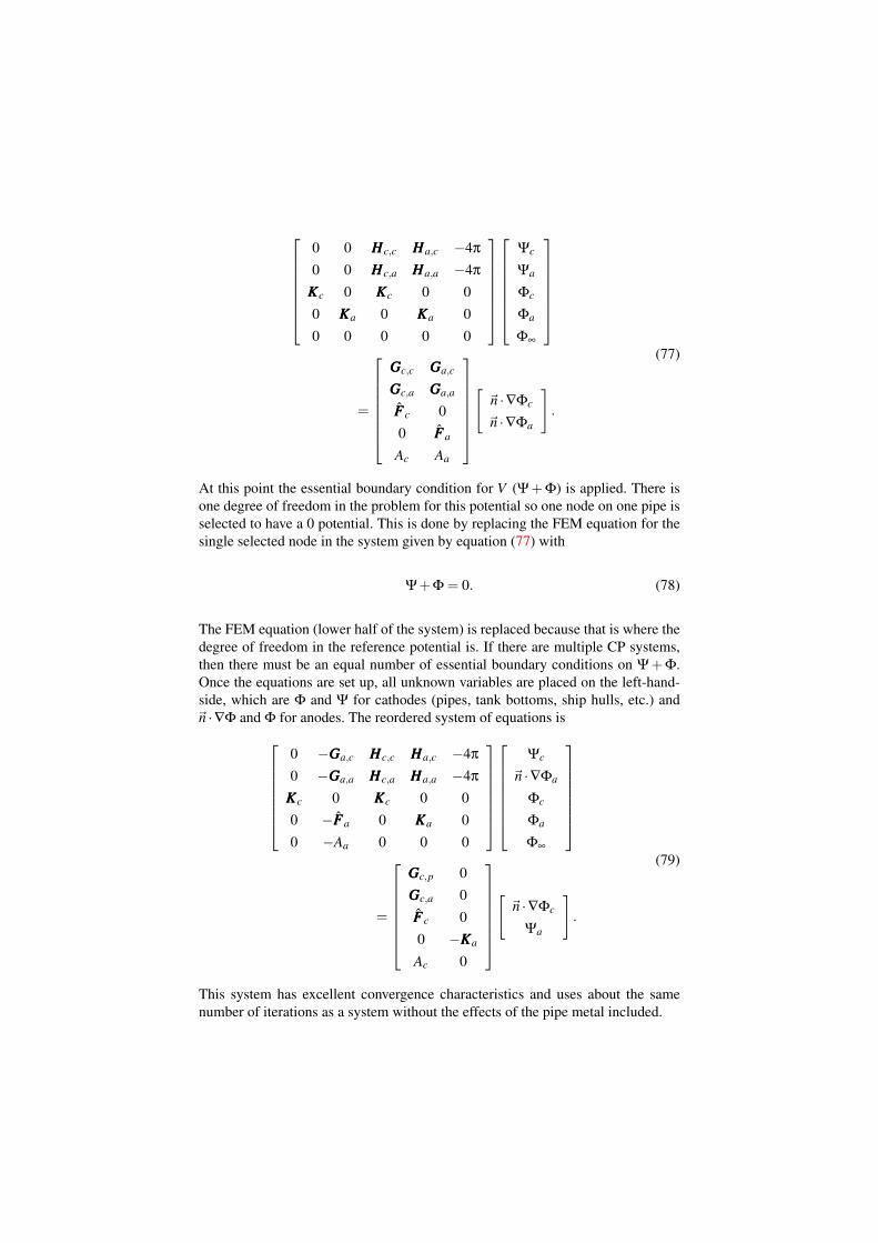
(77)

At this point the essential boundary condition for V (Ψ + Φ) is applied. There isone degree of freedom in the problem for this potential so one node on one pipe isselected to have a 0 potential. This is done by replacing the FEM equation for thesingle selected node in the system given by equation (77) with

Ψ+Φ = 0. (78)

The FEM equation (lower half of the system) is replaced because that is where thedegree of freedom in the reference potential is. If there are multiple CP systems,then there must be an equal number of essential boundary conditions on Ψ + Φ.Once the equations are set up, all unknown variables are placed on the left-hand-side, which are Φ and Ψ for cathodes (pipes, tank bottoms, ship hulls, etc.) and~n ·∇Φ and Φ for anodes. The reordered system of equations is

0 −GGGa,c HHHc,c HHHa,c −4π

0 −GGGa,a HHHc,a HHHa,a −4π

KKKc 0 KKKc 0 00 −FFFa 0 KKKa 00 −Aa 0 0 0

Ψc

~n ·∇Φa

Φc

Φa

Φ∞

=

GGGc,p 0GGGc,a 0FFFc 00 −KKKa

Ac 0

[

~n ·∇Φc

Ψa

].

(79)

This system has excellent convergence characteristics and uses about the samenumber of iterations as a system without the effects of the pipe metal included.

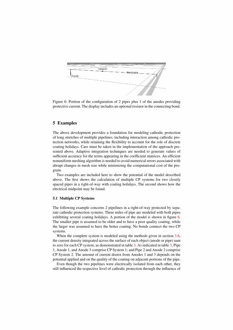
Figure 6: Portion of the configuration of 2 pipes plus 1 of the anodes providingprotective current. The display includes an optional resistor in the connecting bond.

5 Examples

The above development provides a foundation for modeling cathodic protectionof long stretches of multiple pipelines, including interaction among cathodic pro-tection networks, while retaining the flexibility to account for the role of discretecoating holidays. Care must be taken in the implementation of the approach pre-sented above. Adaptive integration techniques are needed to generate values ofsufficient accuracy for the terms appearing in the coefficient matrices. An efficientnonuniform meshing algorithm is needed to avoid numerical errors associated withabrupt changes in mesh size while minimizing the computational cost of the pro-gram.

Two examples are included here to show the potential of the model describedabove. The first shows the calculation of multiple CP systems for two closelyspaced pipes in a right-of-way with coating holidays. The second shows how theelectrical midpoint may be found.

5.1 Multiple CP Systems

The following example concerns 2 pipelines in a right-of-way protected by sepa-rate cathodic protection systems. Three miles of pipe are modeled with both pipesexhibiting several coating holidays. A portion of the model is shown in figure 6.The smaller pipe is assumed to be older and to have a poor quality coating, whilethe larger was assumed to have the better coating. No bonds connect the two CPsystems.

When the complete system is modeled using the methods given in section 3.6,the current density integrated across the surface of each object (anode or pipe) sumto zero for each CP system, as demonstrated in table 3. As indicated in table 3, Pipe1, Anode 1, and Anode 3 comprise CP System 1; and Pipe 2 and Anode 2 compriseCP System 2. The amount of current drawn from Anodes 1 and 3 depends on thepotential applied and on the quality of the coating on adjacent portions of the pipe.

Even though the two pipelines were electrically isolated from each other, theystill influenced the respective level of cathodic protection through the influence of

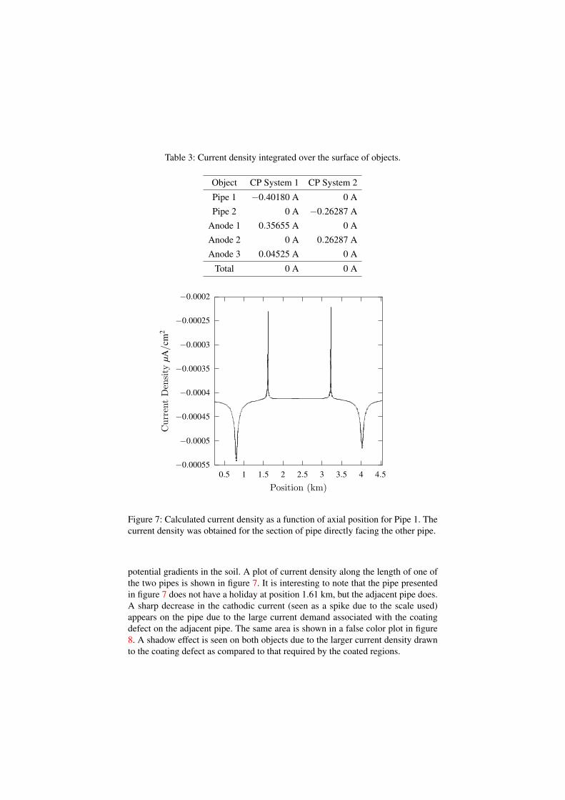
Table 3: Current density integrated over the surface of objects.

Object CP System 1 CP System 2

Pipe 1 −0.40180 A 0 APipe 2 0 A −0.26287 A

Anode 1 0.35655 A 0 AAnode 2 0 A 0.26287 AAnode 3 0.04525 A 0 A

Total 0 A 0 A

−0.00055

−0.0005

−0.00045

−0.0004

−0.00035

−0.0003

−0.00025

−0.0002

0.5 1 1.5 2 2.5 3 3.5 4 4.5

Cur

rent

Den

sity

µA/c

m2

Position (km)

Figure 7: Calculated current density as a function of axial position for Pipe 1. Thecurrent density was obtained for the section of pipe directly facing the other pipe.

potential gradients in the soil. A plot of current density along the length of one ofthe two pipes is shown in figure 7. It is interesting to note that the pipe presentedin figure 7 does not have a holiday at position 1.61 km, but the adjacent pipe does.A sharp decrease in the cathodic current (seen as a spike due to the scale used)appears on the pipe due to the large current demand associated with the coatingdefect on the adjacent pipe. The same area is shown in a false color plot in figure8. A shadow effect is seen on both objects due to the larger current density drawnto the coating defect as compared to that required by the coated regions.

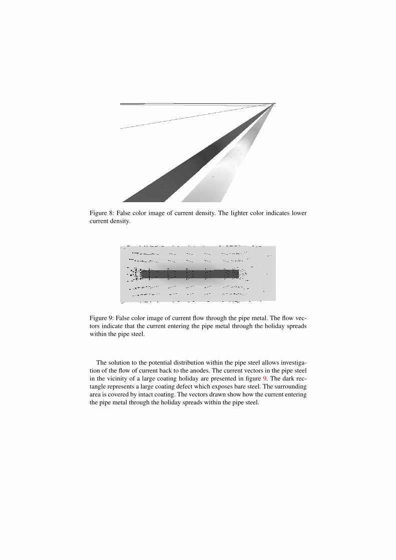
Figure 8: False color image of current density. The lighter color indicates lowercurrent density.

Figure 9: False color image of current flow through the pipe metal. The flow vec-tors indicate that the current entering the pipe metal through the holiday spreadswithin the pipe steel.

The solution to the potential distribution within the pipe steel allows investiga-tion of the flow of current back to the anodes. The current vectors in the pipe steelin the vicinity of a large coating holiday are presented in figure 9. The dark rec-tangle represents a large coating defect which exposes bare steel. The surroundingarea is covered by intact coating. The vectors drawn show how the current enteringthe pipe metal through the holiday spreads within the pipe steel.

−0.35

−0.3

−0.25

−0.2

−0.15

−0.1

−0.05

0

0.05

0.1

1 2 3 4 5 6

Stee

lvo

ltag

e/

V

Position / km

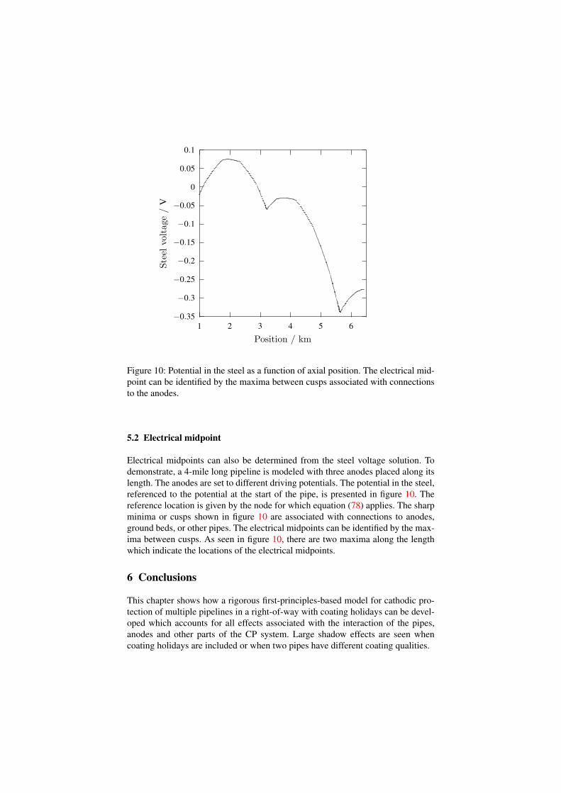
Figure 10: Potential in the steel as a function of axial position. The electrical mid-point can be identified by the maxima between cusps associated with connectionsto the anodes.

5.2 Electrical midpoint

Electrical midpoints can also be determined from the steel voltage solution. Todemonstrate, a 4-mile long pipeline is modeled with three anodes placed along itslength. The anodes are set to different driving potentials. The potential in the steel,referenced to the potential at the start of the pipe, is presented in figure 10. Thereference location is given by the node for which equation (78) applies. The sharpminima or cusps shown in figure 10 are associated with connections to anodes,ground beds, or other pipes. The electrical midpoints can be identified by the max-ima between cusps. As seen in figure 10, there are two maxima along the lengthwhich indicate the locations of the electrical midpoints.

6 Conclusions

This chapter shows how a rigorous first-principles-based model for cathodic pro-tection of multiple pipelines in a right-of-way with coating holidays can be devel-oped which accounts for all effects associated with the interaction of the pipes,anodes and other parts of the CP system. Large shadow effects are seen whencoating holidays are included or when two pipes have different coating qualities.

It should be noted the cathodic protection model requires locally valid polariza-tion curves which describe the chemistry at the pipe-soil interface. The polarizationcurves account for the local soil conditions such as chemistry, coating condition,and anode performance.

Acknowledgements

This work was supported by the Pipeline Research Council International and bythe Gas Research Institute under Contract PR-101-9512.

References

[1] Gas facts - distribution and transmission miles of pipeline.Technical report, American Gas Association, 1999.Http://www.aga.org/StatsStudies/GasFacts/2131.html.

[2] Pipline accident summary report: Pipeline rupture, liquid butane release, andfire, lively, texas august 24 1996. Technical report, National TransportationSafety Board, Washington, D.C., 1998.

[3] Morgan, J., Cathodic Protection. NACE, International: Houston, TX, 2ndedition, 1993.

[4] Wagner, J., Cathodic Protection Design I. NACE, International, Houston,TX, 1994.

[5] Peabody, A.W., Control of Pipeline Corrosion. NACE: Houston, TX, 1978.[6] Newman, J.S., Electrochemical Engineering. Prentice-Hall: Englewood

Cliffs, New Jersey, 2nd edition, 1991.[7] Orazem, M.E., Esteban, J.M., Kenelley, K.J. & Degerstedt, R.M., Mathemat-

ical models for cathodic protection of an underground pipeline with coatingholidays: Part 1 - theoretical development. Corrosion, 53(4), pp. 264–272,1997.

[8] Yan, J.F., Pakalapati, S.N.R., Nguyen, T.V., White, R.E. & Griffin, R.B.,Mathematical modeling of cathodic protection using the boundary elementmethod with a nonlinear polarization curve. Journal of the ElectrochemicalSociety, 139(7), pp. 1932–1936, 1992.

[9] Kennelley, K.J., Bone, L. & Orazem, M.E., Current and potential distributionon a coated pipeline with holidays part i - model and experimental verifica-tion. Corrosion, 49(3), pp. 199–210, 1993.

[10] Nisancioglu, K., Predicting the time dependence of polarization on cathodi-cally protected steel in seawater. Corrosion, 43, pp. 100–111, 1987.

[11] Nisancioglu, K., Gartland, P.O., Dahl, T. & Sander, E., Role of surface struc-ture and flow rate on the polarization of cathodically protected steel in sea-water. Corrosion, 43, pp. 710–718, 1987.

[12] Nisancioglu, K. & Gartland, P.O., Current distribution with dynamic bound-ary conditions. I. Chem. Symposium Series No. 112: Conference on Electro-

chemical Engineering, Loughborough University of Technology: Loughbor-ough, 1989.

[13] Carson, S.L. & Orazem, M.E., Time-dependent polarization of behavior ofpipeline-grade in low ionic strength environments. Journal of Applied Elec-trochemistry, 29, pp. 703–717, 1999.

[14] Anderko, A. & Young, R.D., Model for corrosion of carbon steel in lithiumbromide absorption refrigeration systems. Corrosion, 56(5), pp. 543–555,2000.

[15] Anderko, A., MacKenzie, P. & Young, R.D., Computation of rates of gen-eral corrosion using electrochemical and thermodynamic models. Corrosion,57(3), pp. 202–213, 2001.

[16] Korzhenko, A., Tabellout, M. & Emery, J., Dielectric relaxation properties ofthe polymer coating during its exposition to water. Materials Chemistry andPhysics, 65(3), pp. 253–260, 2000.

[17] Corfias, C., Pebere, N. & Lacabanne, C., Characterization of a thin protectivecoating on galvanized steel by electrochemical impedance spectroscopy and athermostimulated current method. Corrosion Science, 41(8), pp. 1539–1555,1999.

[18] Margarit, I. & Mattos, O., About coatings and cathodic protection: Possi-bilities of impedance as monitoring technique. Electrochemical Methods inCorrosion Research VI, Parts 1 and 2, Transtec Publications: Zurich-Eutikon,pp. 279–292, 1998.

[19] Thompson, I. & Campbell, D., Interpreting nyquist responses from defectivecoatings on steel substrates. Corrosion Science, 36(1), pp. 187–198, 1994.

[20] Bellucci, F. & Nicodemo, L., Water transport in organic coatings. Corrosion,49(3), pp. 235–247, 1993.

[21] Diakow, D., Van Boven, G. & Wilmott, M., Polarization under disbondedcoatings: Conventional and pulsed cathodic protection compared. MaterialsPerformance, 37(5), pp. 17–23, 1998.

[22] Jack, T.R., External corrosion of line pipe - a summary of research activities.Materials Performance, 35(3), pp. 18–24, 1996.

[23] Beavers, J.A. & Thompson, N.G., Corrosion beneath disbonded pipeline.Materials Performance, 36(4), pp. 13–19, 1997.

[24] Riemer, D. & Orazem, M., Development of mathematical models forcathodic protection of multiple pipelines in a right of way. Proceedings of the1998 International Gas Research Conference, Gas Research Institute, GRI:Chicago, p. 117, 1998. Paper TSO-19.

[25] Riemer, D.P. & Orazem, M.E., Cathodic protection of multiple pipelines withcoating holidays. Procedings of the NACE99 Topical Research Symposium:Cathodic Protection: Modeling and Experiment, ed. M.E. Orazem, NACE,NACE International: Houston, TX, pp. 65–81, 1999.

[26] Jones, D.A., Principles and Prevention of Corrosion. Prentice Hall: UpperSaddle River, NJ, 1996.

[27] Carslaw, H.S. & Jaeger, J.C., Conduction of Heat in Solids. Oxford Univer-sity Press: New York, 1959.

[28] Moulton, H.F., Current flow in rectangular conductors. Proceedings of theLondon Mathematical Society, ser. 2(3), pp. 104–110, 1905.

[29] Bowman, F., Introduction to Elliptic Functions with Applications. John Wileyand Sons: New York, 1953.

[30] Orazem, M.E. & Newman, J., Primary current distribution and resistance ofa slotted-electrode cell. Journal of the Electrochemical Society, 131(12), pp.2857–2861, 1984.

[31] Orazem, M.E., Calculation of the electrical resistance of a compact tensionspecimen for crack-propagation measurements. Journal of the Electrochemi-cal Society, 132(9), pp. 2071–2076, 1985.

[32] Orazem, M.E. & Ruch, W., An improved analysis of the potential dropmethod for measuring crack lengths in compact tension specimens. Inter-national Journal of Fracture, 31, pp. 245–258, 1986.

[33] Diem, C.B., Newman, B. & Orazem, M.E., The influence of small machiningerrors on the primary current distribution at a recessed electrode. Journal ofthe Electrochemical Society, 135, pp. 2524–2530, 1988.

[34] Brebbia, C.A. & Dominguez, J., Boundary element methods for potentialproblems. Applied Mathematical Modelling, 1(7), pp. 371–378, 1977.

[35] Aoki, S., Kishimoto, K. & Sakata, M., Boundary element analysis of galvaniccorrosion. Boundary Elements VII, eds. C.A. Brebbia & G. Maier, Springer-Verlag: Heidelberg, volume 1, pp. 73–83, 1985.

[36] Telles, J., Wrobel, L., Mansur, W. & Azevedo, J., Boundary elementsfor cathodic protection problems. Boundary Elements VII, ed. B.C.M. G,Springer-Verlag, volume 1, pp. 63–71, 1985.

[37] Zamani, N. & Chuang, J., Optimal-control of current in a cathodic protectionsystem - a numerical investigation. Optimal Control Applications & Methods,8(4), pp. 339–350, 1987.

[38] Brichau, F. & Deconinck, J., Numerical model for cathodic protection ofburied pipes. Corrosion, 50(1), pp. 39–49, 1994.

[39] Brichau, F., Deconinck, J. & Driesens, T., Modeling of underground cathodicprotection stray currents. Corrosion, 52, pp. 480–488, 1996.

[40] Aoki, S. & Amaya, K., Optimization of cathodic protection system by bem.Engineering Analysis with Boundary Elements, 19(2), pp. 147–156, 1997.

[41] Aoki, S., Amaya, K. & Miyasaka, M., Boundary element analysis of cathodicprotection for complicated structures. Proceedings of the NACE99 TopicalResearch Symposium: Cathodic Protection: Modeling and Experiment, ed.M.E. Orazem, NACE, NACE International: Houston, TX, pp. 45–65, 1999.

[42] Brebbia, C. & Dominguez, J., Boundary Elements: An Introductory Course.McGraw-Hill, The Bath Press: Avon, Great Britain, 1989.

[43] Brebbia, C.A., Telles, J.C.F. & Wrobel, L.C., Boundary Element Techniques.Springer-Verlag: Heidelberg, 1984.

[44] Hartmann, F., Katz, C. & Protopsaltis, B., Boundary elements and symmetry.Ingenieur Archiv, 55(6), pp. 440–449, 1985.

[45] Gray, L. & Paulino, G., Symmetric galerkin boundary integral formulationfor interface and multi-zone problems. International Journal for Numerical

Methods in Engineering, 40, pp. 3085–3101, 1997.[46] Stakgold, I., Greens Functions and Boundary Value Problems. John Wiley &

Sons: New York, 1979.[47] Dwight, H.B., Calculations of resistance to ground. Electrical Engineering,

55, p. 1319, 1936.[48] Telles, J.C.F. & Paula, F.A.D., Boundary elements with equilibrium satisfac-

tion - a consistent formulation for potential and elastostatic analysis. Interna-tional Journal of Numerical Methods in Engineering, 32, pp. 609–621, 1991.

[49] Trevelyan, J. & Hack, H., Analysis of stray current corrosion problems usingthe boundary element method. Boundary Element Technology IX, Computa-tional Mechanics Publications: Boston, pp. 347–356, 1994.

[50] Burton, S., Garbow, K.E., Hillstrom, J.J. & Others, Modified powell methodwith analytic jacobian. Software source code hybrdj.f, 1980. ArgonneNational Laboratory. minpack project. www.netlib.org/minpack.