Modeling menstrual cycle length using a

mixture distribution

YING GUO, AMITA K. MANATUNGA∗

Department of Biostatistics, Emory University, Atlanta, GA, 30322, USA

SHANDE CHEN

Department of Biostatistics, University of North Texas Health Science Center

at Fort Worth,TX, 76107,USA

MICHELE MARCUS

Department of Epidemiology, Emory University, Atlanta, GA, 30322, USA

∗ The corresponding author. Tel: 404-727-1309 Fax: 404-727-1370 Email: amanatu@sph.emory.edu

SUMMARY

In reproductive health studies, epidemiologists are often interested in examining

the effects of covariates on menstrual cycle length which is a convenient, noninvasive

measure of women’s ovarian and reproductive function. Previous literature (Harlow

and Zeger, 1991) suggests that the distribution of cycle length is a mixture of a major

symmetric distribution and a component featuring a long right tail. Motivated by

the shape of this marginal distribution, we propose a mixture distribution for cycle

length, representing standard cycles from a normal distribution and nonstandard cycles

from a shifted Weibull distribution. The parameters are estimated using an estimating

equation derived from the score function of an independence working model. The fitted

mixture distribution agrees well with the distribution estimated using nonparametric

approaches. We propose two measures to help determine whether a cycle is standard

1

or nonstandard, developing tools necessary to identify characteristics of the menstrual

cycles that are biologically indicative of ovarian dysfunction. We model the effect of a

woman’s age on the mean and variation of both standard and nonstandard cycle lengths

using multiple measurements of women.

Key words: Menstrual cycle length; Mixture distribution; Kernel density estimation;

Optimum cutoff; Conditional probability; Estimating equation.

1. INTRODUCTION

Menstrual cycles act as overt indicators of underlying reproductive health. Men-

strual dysfunction may both decrease fertility and increase one’s future risk of various

chronic diseases such as breast cancer, cardiovascular disease and diabetes. Menstrual

cycle characteristics, including cycle length and bleed length, may serve as sensitive and

noninvasive measures of reproductive health. While biological assays have the added

advantage of measuring hormone levels and the potential to estimate the day of ovu-

lation, menstrual cycle characteristics, alone, are easy to observe, cost effective, and

conveniently monitored by women themselves. Altered patterns of menstruation may

indicate subclinical states of reproductive dysfunction and may enable earlier detection

of potential menstrual dysfunction. Our understanding of the endocrinology controlling

menstrual cycles has advanced in recent years. Yen (1991) describes the endocrinology

of the menstrual cycle in terms of three phases including the follicular phase, ovula-

tion and the luteal phase. However, in terms of observable cycle characteristics, there

remains no specific criteria distinguishing normal menstrual function from less severe

forms of dysfunction. Epidemiologists have examined the effects of a range of exposures,

from caffeine consumption and smoking to environmental contaminants, on menstrual

cycle function. Such studies rely on existing and often limited statistical tools for the

analysis of menstrual cycle characteristics.

The statistical analysis of menstrual cycle length is complicated for numerous rea-

sons. First, menstrual cycle lengths are distributed with a long right tail, and the

parametric distribution for cycle length has not been described. Second, sampling bias

will be present if women are followed for a fixed length of time. Women with generally

shorter cycles will be over-represented as they contribute more cycles to the analysis

2

than women with long cycles. Third, depending on the study design, observed cycles

are often censored. For example, if the study ends at a pre-determined time, the last

cycle of most women are right censored. In this paper we aim to develop statistical

tools to address these complexities of menstrual cycle data.

Because the distribution of cycle length consists of both a symmetric part and a

long right tail, it is inadequate to define the distribution with a single symmetric dis-

tribution like the normal distribution. However, researchers have frequently ignored

the non-normality and applied usual regression models for the menstrual cycle length

data. Harlow and colleagues recognized this problem and applied a bipartite model to

analyze menstrual data (Harlow and Zeger, 1991; Harlow et al., 2000). They classified

cycles into two groups: “standard” cycles, those from the symmetric part of the dis-

tribution, and “nonstandard” cycles, those from the long right tail. Standard cycles

are analyzed using Gaussian-assumption based statistical methods such as the repeated

measure analysis of variance. For example, Harlow and Zeger (1991) and Harlow and

Matanoski (1991) defined standard cycles as those less than or equal to 43 days and

used linear random effects models to examine the covariate effects on the mean length

of standard cycles. Lin, Raz and Harlow (1997) extended the linear mixed model to

account for the heterogeneity of within-woman variance of standard cycles. For non-

standard cycles, Harlow et al. (2000) evaluated the age effect on the probability of

having a nonstandard cycle using a generalized estimating equation. A limitation of

the bipartite approach is that the analysis of the cycle length pattern focuses only on

cycles in the symmetric part of the distribution. The analysis of the cycles in the long

right tail is restricted to modeling the probability of having a nonstandard cycle while

the length and variability of nonstandard cycles are not addressed. In other words,

the bipartite modeling approach only utilizes a very small fraction of the information

related to nonstandard cycles.

In this paper our first objective is to develop an appropriate parametric form for the

cycle length marginal distribution that can adequately represent both components of the

observed distribution. Motivated by previous literature (Harlow and Zeger, 1991; Har-

low et al., 2000), we consider a normal and shifted Weibull mixture distribution. There

are several advantages of specifying a parametric form for the marginal distribution :

3

(1) It provides better understanding of the characteristics of cycle lengths, especially

those in the long right tail. (2) It leads to appropriate methods for defining standard

and nonstandard cycles thus facilitating common data analysis used in epidemiology.

(3) It is needed for making correct inferences on the dependence structure among cycles

within women. The second objective of this paper is to model repeated measures of

menstrual cycles of women while maintaining the desired mixture marginal distribu-

tion. Menstrual cycle lengths are known to be distributed differentially among various

sub-populations such as age groups. Through the proposed parametric distribution, we

are able to examine subject-specific covariate effects on both standard and nonstandard

menstrual cycles. Compared to its alternatives, the proposed modeling approach has

the following advantages: first, it doesn’t require the cycles to be categorized by an

arbitrary cutoff as in the bipartite models; secondly, it allows us to target specific as-

pects of the cycle length distribution, such as the mean length and variability; thirdly,

it enables us to differentiate covariate effects on standard and nonstandard menstrual

cycles. This is an appealing feature when modeling covariates such as stress that may

have different influences in the two parts of the distribution (Harlow and Zeger, 1991);

finally, both complete and censored cycles are taken into account in modeling.

In the next section we introduce the reproductive study that motivated this paper.

Some practical issues are discussed regarding menstrual cycle length data. In Section

3, a parametric mixture distribution is proposed. An Independence Working Model

(IWM) (Huster et al., 1989) is used to obtain its parameter estimates. These estimates

are shown to be consistent regardless of the true dependence structure among within-

woman cycle lengths. We also estimate the marginal distribution nonparametrically

and compare it to its parametric counterpart. In Section 4, two methods are developed

for distinguishing standard and nonstandard cycles. In Section 5, a marginal modeling

approach is developed based on the proposed parametric mixture distribution. An

illustration is provided using the reproductive study. We conclude with discussions in

Section 6.

4

2. THE MSSWOW DATA

2.1 Study population

The Mount Sinai Study of Women Office Worker (MSSWOW) was a prospective

cohort study to explore the effects of Video Display Terminal (VDT) use on rates of

spontaneous abortion (Marcus et al., 2000). The participants for the study were re-

cruited between 1991 and 1994 from fourteen companies or government agencies in New

York, New Jersey and Massachusetts. 4640 women office workers completed a cross-

sectional questionnaire. Women between the ages of 18 and 40 were eligible for the

prospective study if they were at risk for pregnancy. This included women who had

sexual intercourse at least once in the past month without using contraception or were

planning to discontinue regular contraceptive use in the next 6 months. 25% of the

qualified women indicated that they were trying to become pregnant. A woman was

excluded if she had already been attempting to conceive a child unsuccessfully for 12

months or longer, if she had a hysterectomy, or if her partner had a vasectomy. Women

were not excluded if they experienced a year or more of attempted pregnancy sometime

in the past. 524 women were finally enrolled in the study. Participants were observed

for one year, or until a clinical pregnancy.

2.2 Definition of menstrual cycles and cycle length

According to WHO standard, a menstrual cycle is defined as the interval from the

first day of one bleeding episode up to and including the day before the next bleeding

episode. During the study, each participant kept a daily diary recording whether men-

strual bleeding occurred, whether they had intercourse and, if so, whether birth control

was used. They also recorded information on specific exposures (e.g., hours of VDT

use) on a daily basis. We excluded those cycles whose starting date or the date when

the bleeding episode began was unrecorded.

As with most other reproductive studies, the MSSWOW data contained incomplete

menstrual cycles during which pregnancy occurred. When a woman becomes pregnant,

5

her reproductive endocrinology changes and the estrogen and progesterone levels do not

decline as in usual non-pregnant cycles. Consequently, the thickened lining of the uterus

is not shed during the pregnancy period and the woman will not experience menstrual

bleeding until delivery or other kinds of pregnancy termination. Therefore, a woman is

temporarily no longer at risk for menstrual bleeding after conception occurs. In other

words, the cycle lengths for pregnancy cycles are inherently missing. For this reason

and the reason that the exact conception date of pregnancy cycles was not available

in the MSSWOW data, clinical or subclinical pregnancy cycles were excluded from our

analysis. We also removed cycles during which hormonal medications were used because

these medications have well known effects on menstrual cycle lengths.

In the MSSWOW data, a cycle was defined as censored if its starting date was

recorded but the ending date was unrecorded. Most of the censored cycles occurred in

the end of the study. A few censored cycles happened during the study when a subject

was too busy or travelling and did not keep the diaries for a period of time.

2.3 Description of the observed menstrual cycle length data

After the exclusions, 3241 menstrual cycles contributed by 444 participants were

included in this analysis. Each woman contributed from 1 to 19 cycles with a median of

10 cycles. Among the 3241 cycles, 2901 were complete and 340 were censored. Women’s

age ranged from 19 to 41 with a median of 31. The observed complete cycle lengths

ranged from 5 to 189 days with the mean of 29.8 days and median of 28 days. Table

1 presents a summary of the observed cycle length distribution characteristics by age

groups. Based on the Tremin Trust data, Harlow et al. (2000) suggested 40 days

is an appropriate cutoff for standard and nonstandard cycles for women across the

reproductive life span. Therefore, we present the observed number of cycles that are

longer than 40 days in our study.

3. ESTIMATION OF THE CYCLE LENGTH DISTRIBUTION

As stated in Section 2, we are interested in characterizing the distribution for menstrual

6

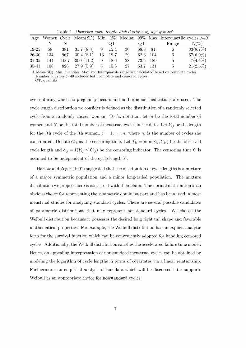
Table 1. Observed cycle length distributions by age groups∗

Age Women Cycle Mean(SD) Min 1% Median 99% Max Interquartile cycles >40N N QT† QT Range N(%)

19-25 58 381 31.7 (8.3) 9 15.4 30 68.8 81 6 33(8.7%)26-30 134 967 30.4 (8.1) 13 19.7 29 62.6 104 6 67(6.9%)31-35 144 1067 30.0 (11.2) 9 18.6 28 73.5 189 5 47(4.4%)35-41 108 826 27.9 (5.9) 5 15.3 27 53.7 131 5 21(2.5%)∗ Mean(SD), Min, quantiles, Max and Interquartile range are calculated based on complete cycles.

Number of cycles > 40 includes both complete and censored cycles.† QT: quantile.

cycles during which no pregnancy occurs and no hormonal medications are used. The

cycle length distribution we consider is defined as the distribution of a randomly selected

cycle from a randomly chosen woman. To fix notation, let m be the total number of

women and N be the total number of menstrual cycles in the data. Let Yij be the length

for the jth cycle of the ith woman, j = 1, . . . , ni where ni is the number of cycles she

contributed. Denote Cij as the censoring time. Let Tij = min(Yij , Cij) be the observed

cycle length and δij = I(Yij ≤ Cij) be the censoring indicator. The censoring time C is

assumed to be independent of the cycle length Y .

Harlow and Zeger (1991) suggested that the distribution of cycle lengths is a mixture

of a major symmetric population and a minor long-tailed population. The mixture

distribution we propose here is consistent with their claim. The normal distribution is an

obvious choice for representing the symmetric dominant part and has been used in most

menstrual studies for analyzing standard cycles. There are several possible candidates

of parametric distributions that may represent nonstandard cycles. We choose the

Weibull distribution because it possesses the desired long right tail shape and favorable

mathematical properties. For example, the Weibull distribution has an explicit analytic

form for the survival function which can be conveniently adopted for handling censored

cycles. Additionally, the Weibull distribution satisfies the accelerated failure time model.

Hence, an appealing interpretation of nonstandard menstrual cycles can be obtained by

modeling the logarithm of cycle lengths in terms of covariates via a linear relationship.

Furthermore, an empirical analysis of our data which will be discussed later supports

Weibull as an appropriate choice for nonstandard cycles.

7

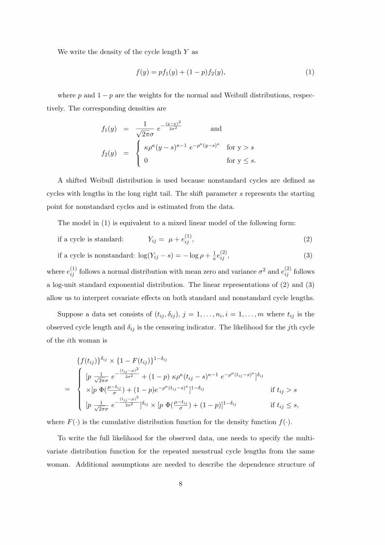
We write the density of the cycle length Y as

f(y) = pf1(y) + (1− p)f2(y), (1)

where p and 1− p are the weights for the normal and Weibull distributions, respec-

tively. The corresponding densities are

f1(y) =1√2πσ

e−(y−µ)2

2σ2 and

f2(y) =

κρκ(y − s)κ−1 e−ρκ(y−s)κfor y > s

0 for y ≤ s.

A shifted Weibull distribution is used because nonstandard cycles are defined as

cycles with lengths in the long right tail. The shift parameter s represents the starting

point for nonstandard cycles and is estimated from the data.

The model in (1) is equivalent to a mixed linear model of the following form:

if a cycle is standard: Yij = µ + e(1)ij , (2)

if a cycle is nonstandard: log(Yij − s) = − log ρ + 1κe

(2)ij , (3)

where e(1)ij follows a normal distribution with mean zero and variance σ2 and e

(2)ij follows

a log-unit standard exponential distribution. The linear representations of (2) and (3)

allow us to interpret covariate effects on both standard and nonstandard cycle lengths.

Suppose a data set consists of (tij , δij), j = 1, . . . , ni, i = 1, . . . , m where tij is the

observed cycle length and δij is the censoring indicator. The likelihood for the jth cycle

of the ith woman is

{f(tij)}δij × {1− F (tij)}1−δij

=

[p 1√2πσ

e−(tij−µ)2

2σ2 + (1− p) κρκ(tij − s)κ−1 e−ρκ(tij−s)κ]δij

×[p Φ(µ−tijσ ) + (1− p)e−ρκ(tij−s)κ

]1−δij if tij > s

[p 1√2πσ

e−(tij−µ)2

2σ2 ]δij × [p Φ(µ−tijσ ) + (1− p)]1−δij if tij ≤ s,

where F (·) is the cumulative distribution function for the density function f(·).

To write the full likelihood for the observed data, one needs to specify the multi-

variate distribution function for the repeated menstrual cycle lengths from the same

woman. Additional assumptions are needed to describe the dependence structure of

8

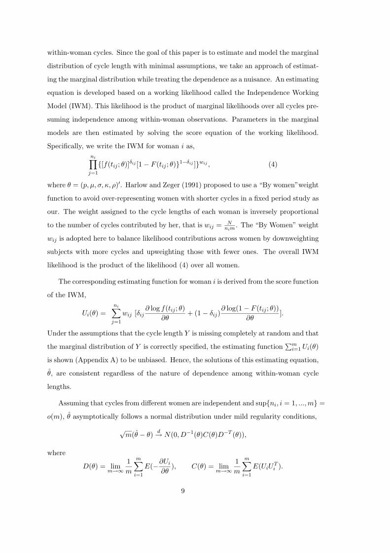
within-woman cycles. Since the goal of this paper is to estimate and model the marginal

distribution of cycle length with minimal assumptions, we take an approach of estimat-

ing the marginal distribution while treating the dependence as a nuisance. An estimating

equation is developed based on a working likelihood called the Independence Working

Model (IWM). This likelihood is the product of marginal likelihoods over all cycles pre-

suming independence among within-woman observations. Parameters in the marginal

models are then estimated by solving the score equation of the working likelihood.

Specifically, we write the IWM for woman i as,ni∏

j=1

{[f(tij ; θ)]δij [1− F (tij ; θ)}1−δij ]}wij , (4)

where θ = (p, µ, σ, κ, ρ)′. Harlow and Zeger (1991) proposed to use a “By women”weight

function to avoid over-representing women with shorter cycles in a fixed period study as

our. The weight assigned to the cycle lengths of each woman is inversely proportional

to the number of cycles contributed by her, that is wij = Nnim

. The “By Women” weight

wij is adopted here to balance likelihood contributions across women by downweighting

subjects with more cycles and upweighting those with fewer ones. The overall IWM

likelihood is the product of the likelihood (4) over all women.

The corresponding estimating function for woman i is derived from the score function

of the IWM,

Ui(θ) =ni∑

j=1

wij [δij∂ log f(tij ; θ)

∂θ+ (1− δij)

∂ log(1− F (tij ; θ))∂θ

].

Under the assumptions that the cycle length Y is missing completely at random and that

the marginal distribution of Y is correctly specified, the estimating function∑m

i=1 Ui(θ)

is shown (Appendix A) to be unbiased. Hence, the solutions of this estimating equation,

θ, are consistent regardless of the nature of dependence among within-woman cycle

lengths.

Assuming that cycles from different women are independent and sup{ni, i = 1, ...,m} =

o(m), θ asymptotically follows a normal distribution under mild regularity conditions,

√m(θ − θ) d→ N(0, D−1(θ)C(θ)D−T (θ)),

where

D(θ) = limm→∞

1m

m∑

i=1

E(−∂Ui

∂θ), C(θ) = lim

m→∞1m

m∑

i=1

E(UiUTi ).

9

One challenging task in fitting this mixture distribution is the choice of the shift

parameter s for the shifted Weibull distribution. The usual likelihood defined as the

product of density evaluated at each observation is in fact a first order approximation

of the true likelihood–the product of probability increments at each observation. When

usual regularity conditions hold, this approximation works well. However, with the

shifted Weibull distribution, the shift parameter represents the lower limit of the Weibull

distribution and the usual likelihood may go to infinity as the shift parameter approaches

the smallest observation, leading to inconsistent estimates of the other parameters. The

corrected likelihood proposed by Cheng and Iles (1987) solved this problem by using

the proper probability increment, instead of density, to calculate the likelihood for

the smallest observation. A profile likelihood approach, based on the corrected IWM

likelihood, is applied to estimate the shift parameter s. For each value of s in the grid,

we maximize the IWM likelihood over the other parameters. The estimate of s is then

chosen as the value corresponding to the maximum profile likelihood and is determined

to be 36 from the data. The estimated shift parameter s is then plugged in the estimating

equation∑m

i=1 Ui(θ) = 0 to obtain the estimates for the other parameters. With the

proposed mixture distribution, the estimating equation does not have explicit solution

and needs to be solved iteratively.

If the shift parameter s is viewed as fixed, the variance for the other parameters can

be readily obtained using the standard sandwich variance estimator. However, since s

is estimated from a particular study, one may need to take into account the uncertainty

in estimating s when making inferences on the other parameters. In this paper, we

use a bootstrap approach for this purpose. Because each woman contributed multiple

cycles to the data, a two-step bootstrapping strategy is applied. We first randomly

select m women with replacement from the data, i.e. i1, i2, . . . , im are chosen such that

ik ∈ {1, . . . , m} for k = 1, . . . ,m. For each of the selected woman ik, we then draw

nik observations with replacement from her observed data: (tikj , δikj), j = 1, . . . , nik .

Using this strategy, 100 bootstrap samples are selected. For each of these samples, the

shift parameter s and the other parameters in the mixture distribution are estimated

using the procedure described earlier. Bootstrap variance estimators are obtained from

bootstrap parameter estimates. Normal approximation is used for hypothesis testing

and the validity of the approximation is confirmed by Q-Q plots.

10

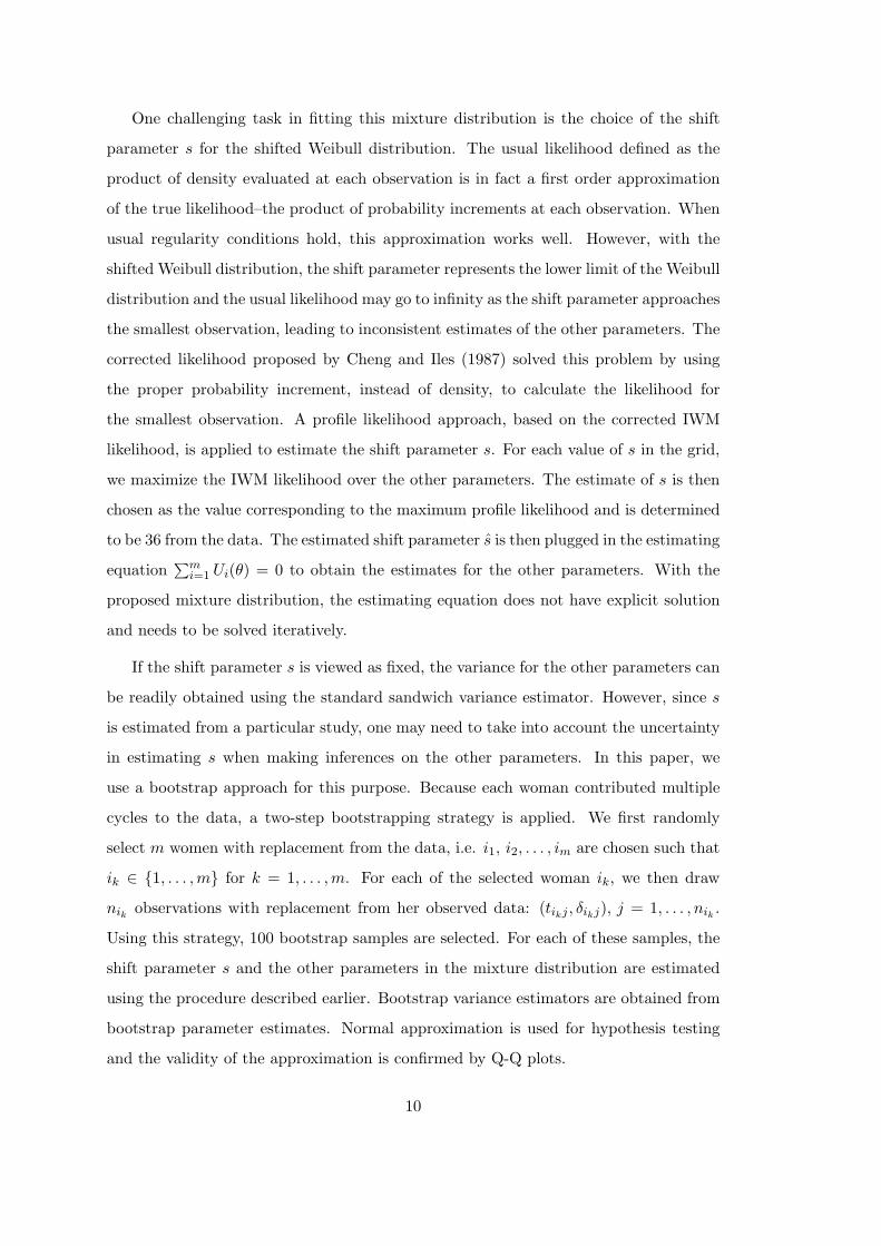
Table 2. Estimated mean and standard deviation of standard and nonstandard cyclesWomen cycle standard cycle nonstandard cycle on the scale of log(Y − s)

N N mean std.† mean (geometric mean of Y∗) std.†

days days log(days) log(days)age group19-25 58 381 30.44 4.79 2.56 (48.94) 0.7926-30 134 967 28.81 3.37 1.74 (41.70) 1.2831-35 144 1067 28.63 3.56 2.37 (46.70) 1.4035-41 108 826 27.55 3.98 1.60 (40.95) 1.63all women 444 3241 28.59 3.83 1.99 (43.30) 1.36∗ geometric mean of Y is obtained by taking exponential of the mean of log(Y-s)and adjust for the shift.† std. represents standard deviation.

Table 2 presents the estimated mean and standard deviation of both standard and

nonstandard cycles for all women and for each 5-year age subgroup. The mean and

standard deviation for nonstandard cycles are presented on the log-scale and they can

be transformed to the original scale for meaningful interpretations. One observation

from Table 2 is that the mean of the normal distribution decreases with the increase

of women’s age. Women’s age also seems to have a quadratic effect on the variation of

standard cycles. For nonstandard cycles, there is no clear trend in mean cycle length

but the variation increases linearly with age. According to the parameter estimates in

Table 2, the probabilities for a cycle length to be greater than 40 are 8.6%, 7.0%, 4.6%

and 3.0% in ascending order of age, which are very close to the observed proportions in

Table 1.

To examine the validity of the shifted Weibull distribution, diagnostic plots are

obtained using cycles with lengths greater than the estimated shift parameter s =

36. The Kaplan-Meier estimate S is obtained and the plot of log(−log(S(t − 36)))

versus log(t − 36) yields a fairly straight line, indicating the Weibull distribution is an

appropriate choice for nonstandard cycles. Similar diagnostic plots are obtained with

cycles greater than 40 days.

To determine the appropriateness of the fitted parametric mixture distribution, we

estimate the marginal distribution of menstrual cycle lengths nonparametrically. Harlow

and Zeger (1991) proposed a nonparametric method based on kernel density estimation.

11

The density estimator for complete cycles is

f(x) =1

N∗

m∑

i=1

n∗i∑

j=1

wij K(x− tij

h),

where wij is the ”By-Women” weight assigned to each cycle. n∗i is the number of

complete cycles contributed by the ith women. N∗ is the total number of complete

cycles for all women. The variable x is the cycle length (in days) for which the kernel

density is estimated. In this paper, a normal density kernel K is applied. The bandwidth

h is decided with the maximum likelihood cross-validation method (Hardle, 1990). To

adjust for censored cycles, the Monte Carlo EM algorithm is used for the kernel density

estimator (Harlow and Zeger, 1991).

As an alternative, we propose a nonparametric approach based on Kaplan-Meier

estimates. Assuming that within-woman cycle lengths are independent and identically

distributed conditional on a given woman, we first obtain the Kaplan-Meier estimates

Si, i = 1, . . . , m for each individual woman based on the multiple cycle lengths she

contributed. Then, the overall Kaplan-Meier survival function estimate for cycle length

is defined as,

SKM (t) =1m

m∑

i=1

Si(t).

In this way, each woman contributes equally in calculating the overall Kaplan-Meier

estimates. Based on SKM , kernel density estimation is applied to obtain the smoothed

density estimates. Let tg (g = 1, . . . , G) denote the gth distinct cycle length when the

complete cycles from all the women are sorted. Denote 4SKM (tg) as the amount of

jump at time tg in SKM , i.e.

4SKM (tg) = SKM (t−g )− SKM (tg).

The Kaplan-Meier density estimate for cycle length is

f(x) =G∑

g=1

4SKM (tg) K(x− tg

h).

The proposed Kaplan-Meier method yields very similar density estimates as the

kernel density estimation method by Harlow and Zeger. The advantages of the Kaplan-

Meier method are that it does not require iterations in computation to handle censored

12

observations and is much easier to apply with contemporary statistical softwares such

as SAS or SPSS.

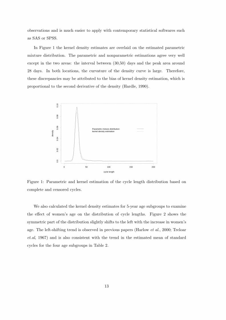
In Figure 1 the kernel density estimates are overlaid on the estimated parametric

mixture distribution. The parametric and nonparametric estimations agree very well

except in the two areas: the interval between (30,50) days and the peak area around

28 days. In both locations, the curvature of the density curve is large. Therefore,

these discrepancies may be attributed to the bias of kernel density estimation, which is

proportional to the second derivative of the density (Hardle, 1990).

cycle length

dens

ity

0 50 100 150 200

0.0

0.02

0.04

0.06

0.08

0.10

Parametric mixture distribution kernel density estimation

Figure 1: Parametric and kernel estimation of the cycle length distribution based on

complete and censored cycles.

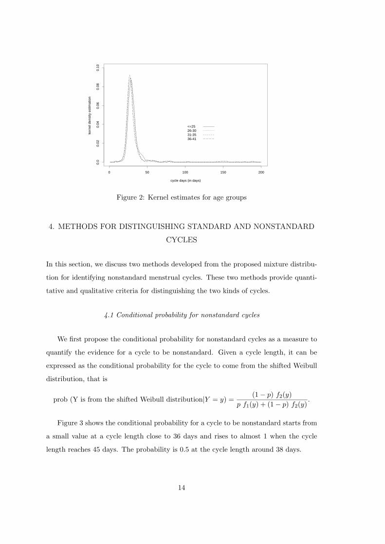
We also calculated the kernel density estimates for 5-year age subgroups to examine

the effect of women’s age on the distribution of cycle lengths. Figure 2 shows the

symmetric part of the distribution slightly shifts to the left with the increase in women’s

age. The left-shifting trend is observed in previous papers (Harlow et al., 2000; Treloar

et.al, 1967) and is also consistent with the trend in the estimated mean of standard

cycles for the four age subgroups in Table 2.

13

cycle days (in days)

kern

el d

ensi

ty e

stim

atio

n

0 50 100 150 200

0.0

0.02

0.04

0.06

0.08

0.10

<=2526-3031-3536-41

Figure 2: Kernel estimates for age groups

4. METHODS FOR DISTINGUISHING STANDARD AND NONSTANDARD

CYCLES

In this section, we discuss two methods developed from the proposed mixture distribu-

tion for identifying nonstandard menstrual cycles. These two methods provide quanti-

tative and qualitative criteria for distinguishing the two kinds of cycles.

4.1 Conditional probability for nonstandard cycles

We first propose the conditional probability for nonstandard cycles as a measure to

quantify the evidence for a cycle to be nonstandard. Given a cycle length, it can be

expressed as the conditional probability for the cycle to come from the shifted Weibull

distribution, that is

prob (Y is from the shifted Weibull distribution|Y = y) =(1− p) f2(y)

p f1(y) + (1− p) f2(y).

Figure 3 shows the conditional probability for a cycle to be nonstandard starts from

a small value at a cycle length close to 36 days and rises to almost 1 when the cycle

length reaches 45 days. The probability is 0.5 at the cycle length around 38 days.

14

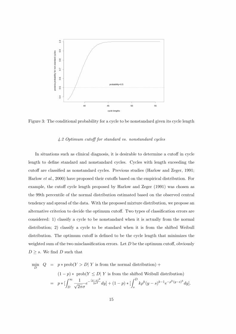
cycle lengths

post

eria

pro

babi

ltiy

for

non-

stan

dard

cyc

les

40 45 50 55

0.4

0.5

0.6

0.7

0.8

0.9

1.0

probability=0.5

Figure 3: The conditional probability for a cycle to be nonstandard given its cycle length

4.2 Optimum cutoff for standard vs. nonstandard cycles

In situations such as clinical diagnosis, it is desirable to determine a cutoff in cycle

length to define standard and nonstandard cycles. Cycles with length exceeding the

cutoff are classified as nonstandard cycles. Previous studies (Harlow and Zeger, 1991;

Harlow et al., 2000) have proposed their cutoffs based on the empirical distribution. For

example, the cutoff cycle length proposed by Harlow and Zeger (1991) was chosen as

the 99th percentile of the normal distribution estimated based on the observed central

tendency and spread of the data. With the proposed mixture distribution, we propose an

alternative criterion to decide the optimum cutoff. Two types of classification errors are

considered: 1) classify a cycle to be nonstandard when it is actually from the normal

distribution; 2) classify a cycle to be standard when it is from the shifted Weibull

distribution. The optimum cutoff is defined to be the cycle length that minimizes the

weighted sum of the two misclassification errors. Let D be the optimum cutoff, obviously

D ≥ s. We find D such that

minD

Q = p ∗ prob(Y > D| Y is from the normal distribution) +

(1− p) ∗ prob(Y ≤ D| Y is from the shifted Weibull distribution)

= p ∗ [∫ ∞

D

1√2πσ

e−(y−µ)2

2σ2 dy] + (1− p) ∗ [∫ D

skρk(y − s)k−1e−ρk(y−s)k

dy].

15

Using the parameter estimates of model (1), we calculate the misclassification prob-

ability Q and find the optimum cutoff to be 38 days. In fact, Figure 4 shows that any

cutoff between 36 and 45 will result in very small misclassification probabilities.

cutoff point

mis

spec

ifica

tion

prob

abili

ty

30 35 40 45 50 55

0.1

0.2

0.3

0.4

Figure 4: The optimum cutoff cycle length

One interesting observation is that the conditional probability for a cycle to non-

standard is 0.5 at the cycle length of 38 days. Therefore, cycles that are classified as

nonstandard by the optimum cutoff are those that have greater conditional probability

to be nonstandard than to be standard. In this respect, the conditional probability

method and the optimum cutoff approach agree well.

5. MODELING COVARIATES

One major task in the analysis of menstrual data is to investigate covariate effects on

menstrual cycle lengths. In this paper, we focus on modeling the mean and variability

of cycle lengths. These two attributes of the distribution are important indicators of

the menstrual function and have been frequently investigated (Treloar et al., 1967;

Lin, Raz and Harlow, 1997). With the proposed mixture distribution, the mean and

variation of standard and nonstandard cycles are summarized by the parameters of the

two component distributions. The covariate effects on the two kinds of cycles can then

be modelled simultaneously through the corresponding parameters.

16

Marginally, the cycle length Y is assumed to follow the proposed mixture distribution

with the density function defined in (1),

f(y) = p f1(y; µi, σi) + (1− p) f2(y; s, κi, ρi),

where f1 and f2 are the densities for the normal and shifted Weibull distributions,

respectively. Due to the considerable complexity in estimating the shift parameter s,

we do not model it in terms of covariates but rather estimate it from all the data. The

proportion parameter p in the mixture distribution is not modelled due to our focus on

the mean and variation.

Let xi denote the vector of covariates of interest for the ith woman. Here, we choose

women’s age as the covariate to illustrate the modeling approach. Based on observations

from Table 2, we model the mean and variance of standard cycles using a linear and

a quadratic model, respectively. In the quadratic model, ages are centered around the

median age in the data set. The models for standard cycles are then

µi = β0 + β1 xi, and

log(σ2i ) = α0 + α1 (xi − 31) + α2 (xi − 31)2.

For nonstandard cycles, let η and υ denote the mean and variance for the logarithm

of the shifted Weibull distribution. The mean η is modeled with distinct parameters for

the four age subgroups in Table 2. A Wald test is used to test the homogeneity of the

four age-specific means. A linear model is fitted for the variance υ,

ηi = η(1)I(xi≤25) + η(2)I(26≤xi≤30) + η(3)I(31≤xi≤35) + η(4)I(36≤xi≤41), and

log(υi) = γ0 + γ1 xi,

where I is an indicator variable. The estimating equation based on the IWM is used to

obtain parameter estimates and the standard errors are estimated using the bootstrap

approach described in Section 3. Table 3 summarizes the results. In comparison, we

also report the sandwich variance estimator of the estimating equation where s is as-

sumed to be fixed. As expected, the bootstrap standard errors are slightly larger than

the sandwich standard errors due to the variability in estimating s. The Q-Q plots

confirm the bootstrap parameter estimates approximately follow normal distributions.

Therefore, the normal approximation is used for hypothesis testing.

17

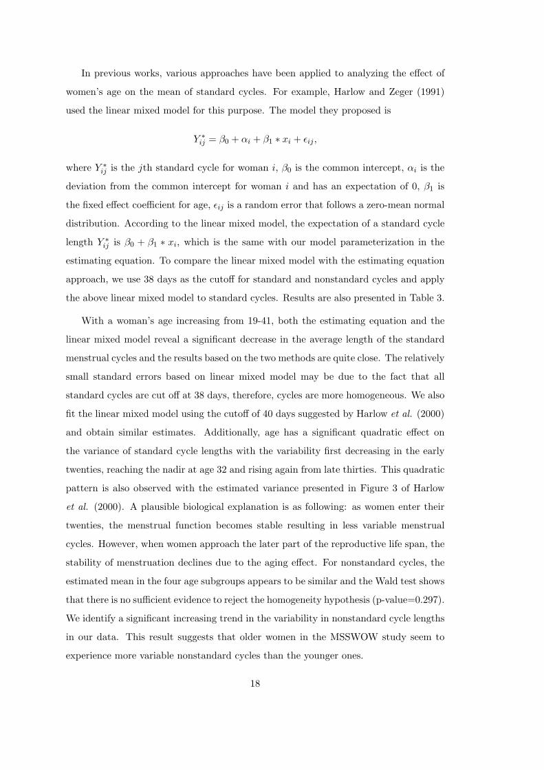
In previous works, various approaches have been applied to analyzing the effect of

women’s age on the mean of standard cycles. For example, Harlow and Zeger (1991)

used the linear mixed model for this purpose. The model they proposed is

Y ∗ij = β0 + αi + β1 ∗ xi + εij ,

where Y ∗ij is the jth standard cycle for woman i, β0 is the common intercept, αi is the

deviation from the common intercept for woman i and has an expectation of 0, β1 is

the fixed effect coefficient for age, εij is a random error that follows a zero-mean normal

distribution. According to the linear mixed model, the expectation of a standard cycle

length Y ∗ij is β0 + β1 ∗ xi, which is the same with our model parameterization in the

estimating equation. To compare the linear mixed model with the estimating equation

approach, we use 38 days as the cutoff for standard and nonstandard cycles and apply

the above linear mixed model to standard cycles. Results are also presented in Table 3.

With a woman’s age increasing from 19-41, both the estimating equation and the

linear mixed model reveal a significant decrease in the average length of the standard

menstrual cycles and the results based on the two methods are quite close. The relatively

small standard errors based on linear mixed model may be due to the fact that all

standard cycles are cut off at 38 days, therefore, cycles are more homogeneous. We also

fit the linear mixed model using the cutoff of 40 days suggested by Harlow et al. (2000)

and obtain similar estimates. Additionally, age has a significant quadratic effect on

the variance of standard cycle lengths with the variability first decreasing in the early

twenties, reaching the nadir at age 32 and rising again from late thirties. This quadratic

pattern is also observed with the estimated variance presented in Figure 3 of Harlow

et al. (2000). A plausible biological explanation is as following: as women enter their

twenties, the menstrual function becomes stable resulting in less variable menstrual

cycles. However, when women approach the later part of the reproductive life span, the

stability of menstruation declines due to the aging effect. For nonstandard cycles, the

estimated mean in the four age subgroups appears to be similar and the Wald test shows

that there is no sufficient evidence to reject the homogeneity hypothesis (p-value=0.297).

We identify a significant increasing trend in the variability in nonstandard cycle lengths

in our data. This result suggests that older women in the MSSWOW study seem to

experience more variable nonstandard cycles than the younger ones.

18

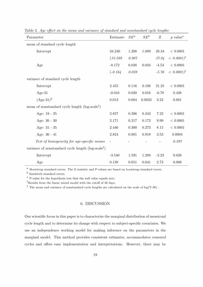
Table 3. Age effect on the mean and variance of standard and nonstandard cycle lengths

Parameter Estimate SEa SEb Z p value?

mean of standard cycle length

Intercept 34.240 1.208 1.089 28.34 < 0.0001

(33.589 0.907 37.04 < 0.0001)†

Age -0.172 0.038 0.034 -4.53 < 0.0001

(-0.164 0.028 -5.76 < 0.0001)†

variance of standard cycle length

Intercept 2.455 0.116 0.106 21.25 < 0.0001

Age-31 -0.016 0.020 0.016 -0.78 0.438

(Age-31)2 0.013 0.004 0.0033 3.22 0.001

mean of nonstandard cycle length (log-scale‡)

Age: 19 - 25 2.857 0.396 0.343 7.22 < 0.0001

Age: 26 - 30 2.171 0.217 0.172 9.99 < 0.0001

Age: 31 - 35 2.446 0.300 0.273 8.15 < 0.0001

Age: 36 - 41 2.824 0.801 0.919 3.53 0.0004

Test of homogeneity for age-specific means - - - - 0.297

variance of nonstandard cycle length (log-scale‡)

Intercept -3.540 1.591 1.288 -2.23 0.026

Age 0.138 0.051 0.041 2.73 0.006

a Bootstrap standard errors. The Z statistic and P-values are based on bootstrap standard errors.b Sandwich standard errors.? P-value for the hypothesis test that the null value equals zero.†Results from the linear mixed model with the cutoff of 38 days.‡ The mean and variance of nonstandard cycle lengths are calculated on the scale of log(Y-36) .

6. DISCUSSION

Our scientific focus in this paper is to characterize the marginal distribution of menstrual

cycle length and to determine its change with respect to subject-specific covariates. We

use an independence working model for making inference on the parameters in the

marginal model. This method provides consistent estimates, accommodates censored

cycles and offers easy implementation and interpretations. However, there may be

19

an efficiency loss in using this approach particularly with strong dependence among

within-woman cycles. In addition, this marginal approach is not applicable if one is

interested in cycle-specific prediction or longitudinal effects. In such a case, additional

assumptions regarding the dependence structure are required. A possible extension

of the proposed approach is to include a random effect αi in both the normal and

shifted Weibull components of the mixture distribution to account for the within-woman

correlation. More specifically, one can add αi in (2) and a scaled αi in (3). Under

the assumptions that within-woman cycle lengths are independent conditional on the

random effect and that the random effect follows a normal distribution, a full likelihood

can be constructed. Since the marginal likelihood does not have an explicit form in this

case, EM algorithm or Gibbs sampler is needed for the parameter estimates. It should

be noted that the random effects model permits a mixture distribution conditional

on the random effect. However, the unconditional or marginal distribution will not

have the same form of a mixture marginal distribution that we have focussed in this

paper. Alternatively, one can model the repeated measures of menstrual cycle lengths

using a copula model. Let Y1, . . . , Yni represent cycle lengths from woman i. The joint

survival function can be defined from marginals through a copula. For example, if an

Archimedean copula φ is used,the joint survivor function is

S(y1, . . . , yni) = φ−1{φ(S1(y1)), . . . , φ(Sni(yni))}.

In this case, the marginal survival functions S1, . . . , Sni can specified as proposed mix-

ture distributions. The dependence among within-woman cycle lengths is characterized

by the copula φ. This approach will allow modelling the dependence structure while

maintaining the desired mixture marginal distributions.

Harlow and Zeger (1991) and Harlow et al. (2000) proposed 43 and 40 days, re-

spectively, as the cutoffs for standard and nonstandard cycles. They determined cutoffs

based on the empirical normal distribution and focused on reducing one of the misclas-

sification errors: classify a standard cycle as nonstandard. The optimum cutoff that

we propose is based on both components of the mixture distribution and is defined to

minimize the sum of both misclassification errors. Due to the difference in the criteria,

the 38 days optimum cutoff we suggest is shorter than theirs. The optimum cutoff may

change with age (Harlow et al., 2000). Since two thirds of the subjects in our study

20

were within the age of 26-35, the 38 days cutoff may not be generalizable to women

across the entire reproductive life span, especially to the years close to the menarche

and menopause.

The majority of prior studies on menstrual cycles are focused on standard cycles.

With the mixture distribution, we are now able to probe into the field of nonstandard

cycles. However, one needs to be cautious of the fact that the number of nonstandard

cycles in healthy women is generally much smaller than the number of standard ones.

Furthermore, the length of nonstandard cycles has a much wider range and is more

variable than that of standard cycles. Consequently, a small data set with few extra

long cycles may result in unstable estimates of the parameters for the shifted Weibull

distribution.

In strict terms, nonstandard cycles include cycles that are either atypically long or

atypically short, though nonstandard long cycles are generally much more common than

nonstandard short cycles. Harlow et al. (2000) suggested that nonstandard short cycles

are most likely to exist in older women resulting from phenomena of intermenstrual

bleeding and polymenorrhea. In this paper, we only consider nonstandard cycles in the

long right tail because the number of extremely short cycles in our data set is too small

to be used for valid analysis.

The attributes of the menstrual cycle length distribution are related to the subject

characteristics of the study population. The subject age range of the MSSWOW study

is 19-41. Thus, women close to menarche or menopause are not represented. Since it is

known that the menstrual cycle is more variable close to menarche and menopause, the

results in this paper may not be generalized to women beyond the age range examined

here. Another feature of the MSSWOW data is that the population for this study was

selected because they were “at risk” of pregnancy and 25% of these women identified

themselves as trying to become pregnant. The attributes of the distribution may also

be affected by the study design. For example, the cycle length variability observed with

the MSSWOW data (Table 1) is greater than that in the Tremin Trust data (Treloar

et.al, 1967; Harlow et.al, 2000) but is not different from other studies (e.g. Chiazze

et.al, 1968). A plausible explanation is that the Tremin Trust data is based on women

that were followed over many years while the subjects in both Chiazze et al. (1968)

21

and MSSWOW data were followed for only one or two years. Women who participate

in many years of diary keeping may be a population with more regular cycles.

The definitions of standard and nonstandard cycles in this paper are based on the

menstrual cycle length and differ from the concepts of “normal” and “abnormal” cycles

in the biological sense. To determine whether a cycle is “abnormal” or not, one would

need to measure hormone levels or use other techniques that directly monitor ovarian

function. It is likely that menstrual cycles, like other physiologic indicators, are best

described on a continuous scale rather than a discrete one, i.e. “normal” and “abnor-

mal”. The aim of this paper is to develop statistical tools that will enable researchers to

make better use of menstrual cycle data as indicators of underlying biological function.

One of the reviewers pointed out the potential problem of informative censoring on

cycle length due to pregnancy. There are several challenging issues in addressing this

problem. First, the censoring time, which is the conception time, is very difficult to

obtain in practice because the conception date can only be measured with error using

techniques such as ultrasound or be approximated through back calculation based on a

gestational period of 40 weeks. In the MSSWOW data as well as many other reproduc-

tive studies, the conception dates are not available. Second, even when the conception

time is measured, there are additional difficulties in adjusting for the potential depen-

dent censoring due to pregnancy. For example, when the conception occurs, a woman’s

risk for the event, which is the occurrence of menstrual bleeding, becomes zero due to

the change in her reproductive endocrinology. More complex statistical methods with

additional assumptions regarding the censoring mechanism are needed to address these

issues related to pregnancy cycles.

ACKNOWLEDGEMENT

This work was supported by NIH grants, R01-ES012458-01 and R01-HD24618, and a

grant from the University Research Committee of Emory University. We are grateful

to the referees and editors for constructive suggestions that have significantly improved

this paper. We also thank Chanley Small for her helpful comments in revising the

manuscript.

22

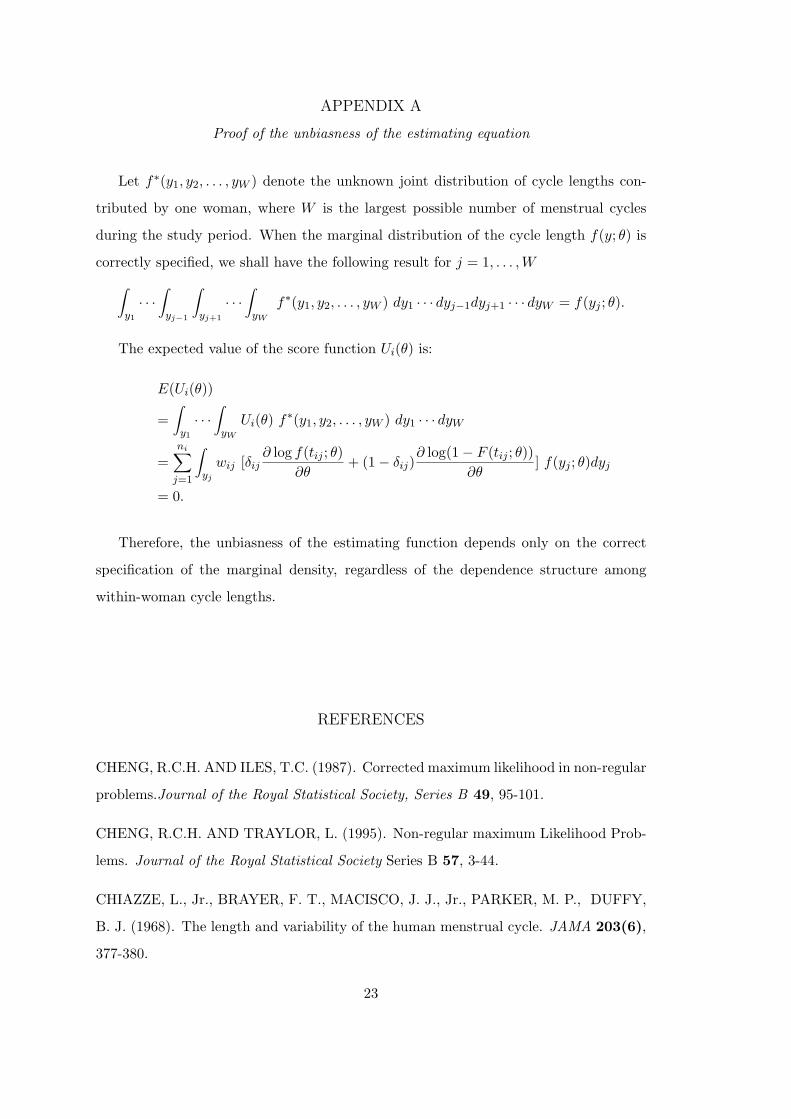
APPENDIX A

Proof of the unbiasness of the estimating equation

Let f∗(y1, y2, . . . , yW ) denote the unknown joint distribution of cycle lengths con-

tributed by one woman, where W is the largest possible number of menstrual cycles

during the study period. When the marginal distribution of the cycle length f(y; θ) is

correctly specified, we shall have the following result for j = 1, . . . ,W

∫

y1

· · ·∫

yj−1

∫

yj+1

· · ·∫

yW

f∗(y1, y2, . . . , yW ) dy1 · · · dyj−1dyj+1 · · · dyW = f(yj ; θ).

The expected value of the score function Ui(θ) is:

E(Ui(θ))

=∫

y1

· · ·∫

yW

Ui(θ) f∗(y1, y2, . . . , yW ) dy1 · · · dyW

=ni∑

j=1

∫

yj

wij [δij∂ log f(tij ; θ)

∂θ+ (1− δij)

∂ log(1− F (tij ; θ))∂θ

] f(yj ; θ)dyj

= 0.

Therefore, the unbiasness of the estimating function depends only on the correct

specification of the marginal density, regardless of the dependence structure among

within-woman cycle lengths.

REFERENCES

CHENG, R.C.H. AND ILES, T.C. (1987). Corrected maximum likelihood in non-regular

problems.Journal of the Royal Statistical Society, Series B 49, 95-101.

CHENG, R.C.H. AND TRAYLOR, L. (1995). Non-regular maximum Likelihood Prob-

lems. Journal of the Royal Statistical Society Series B 57, 3-44.

CHIAZZE, L., Jr., BRAYER, F. T., MACISCO, J. J., Jr., PARKER, M. P., DUFFY,

B. J. (1968). The length and variability of the human menstrual cycle. JAMA 203(6),

377-380.

23

EVERITT, B.S. (1984). Maximum likelihood estimation of the parameters in a mix-

ture of two univariate normal distributions; a comparison of different algorithms. The

Statistician 33, 205-215.

HARLOW, S.D. AND ZEGER, S.L. (1991). An application of longitudinal methods to

the analysis of menstrual diary data. Journal of Clinical Epidemiology 44, 1015-1025.

HARLOW, S.D., LIN, X. AND HO, M.J. (2000). Analysis of menstrual diary data

across the reproductive life span Applicability of the bipartite model approach and the

importance of within-woman variance. Journal of Clinical Epidemiology 53, 722-733.

HARLOW, S.D. AND MATANOSKI, G.M. (1991). The association between weight,

physical activity, and stress and variation in the length of the menstrual cycle. American

Journal of Epidemiology 133, 38-49.

HARDLE, W. (1990). Smoothing techniques with implementation in S. New York:

Springer-Verlag.

HUSTER, W., BROOKMEYER, R. and SELF, S.G. (1989). Modelling paired survival

data with covariates. Biometrics 45, 145-156.

KLEIN, J.P. AND MOESCHBERGER, M. L. (1997). Survival Analysis: Techniques

for censored and truncated data. New York: Springer-Verlag.

LIN, X., RAZ, J. AND HARLOW, S.D. (1997). Linear mixed models with heteroge-

neous within-cluster variances. Biometrics 53, 910-923.

MARCUS, M., MCCHESNEY, R., GOLDEN, A. AND LANDRIGAN, P. (2000). Video

Display Terminals and miscarriages. Journal of the American Medical Women’s Asso-

ciation 55, 84-88.

MURPHY, S.A., BENTLEY, G.R. AND O’HANESIAN, M.A. (1995). An analysis for

menstrual data with time-varying covariates. Statistics in Medicine 14, 1843-1857.

TRELOAR, A.E., BOYNTON, R.E., BEHN, B.G. and BROWN, B.W. (1967). Varia-

tion of the human menstrual cycle through reproductive life. International Journal of

Fertility 12, 77-126.

24

WANG, M.C. AND CHANG, S.H. (1999). Nonparametric estimation of a recurrent

survival function. Journal of the American Statistical Association 94, 146-153.

YEN, S.S.C. (1991). The human menstrual cycle: neuroendocrine regulation. in Yen,

S.S.C. and Jaffe, R.B.. Reproductive endocrinology . Philadelphia: W.B. Saunders

Company. 273-308.

25

LIST OF TABLES AND FIGURE CAPTIONS

Tables

• Table 1. Observed cycle length distributions by age groups

• Table 2. Estimated mean and standard deviation of standard and nonstandard

cycles.

• Table 3. Age effect on the mean and variance of standard and nonstandard cycle

lengths.

Figures

• Figure 1. Parametric and kernel estimation of the cycle length distribution based

on complete and censored cycles.

• Figure 2. Kernel estimates for age groups.

• Figure 3. The conditional probability for a cycle to be nonstandard given its cycle

length.

• Figure 4. The optimum cutoff cycle length.

26