MODELING OF MAGNETIC SURFACE PROBE

USING JMAG SOFTWARE AND APPLICATION

OF MAGNETIC METHODS FOR

CHARACTERISATION OF BOILER TUBES

A thesis submitted in partial fulfillment of the requirements for

the award of the degree of

M.Tech

in

Non-Destructive Testing

By

SHAIK SHAHAZAD

213112012

D E PA RT M E NT OF PHY S I C S

N AT I ON A L IN S T I T UT E OF T E C HN OLOGY

T I R U C HI R A P PA L L I– 6200 15

D E C E MB E R 2 01 3

BONAFIDE CERTIFICATE

This is to certify that the project titled “Modeling of Magnetic Surface Probe Using

JMAG Software and Application of Magnetic Methods for Characterization of Boiler

Tubes” is a bonafide record of the work done by

SHAIK SHAHAZAD (213112012)

in partial fulfillment of the requirements for the award of the degree of Master of

Technology in Non-Destructive Testing of the NATIONAL INSTITUTE OF

TECHNOLOGY, TIRUCHIRAPPALLI, during the year 2013-2014.

Dr. A. CHANDRA BOSE

Head,

Department of Physics,

National Institute of Technology,

Tiruchirappalli - 620015

Project Viva-voce held on _____________________________

Internal Examiner External Examiner

Dr. N.GOPALAKRISHNAN

Associate Professor,

Department of Physics,

National Institute of Technology,

Tiruchirappalli - 620015

Dr. RAJAT K ROY

External guide,

Scientist, NDE & Magnetic Material Group,

MST Division

CSIR - National Metallurgical Laboratory,

Jamshedpur – 831007, India.

i

ABSTRACT

A magnetic sensing probe that can evaluate the magnetic hysteresis loop of a

ferro magnetic material is designed on the principle of Faraday’s laws of

electromagnetic induction and simulation is done with the help of JMAG software to

optimize the probe parameters such as probe dimensions and windings. The 9Cr-1Mo

material is tempered at different temperatures after quenching, and different material

properties such as microstructural, mechanical and magnetic properties were

evaluated. Boiler tubes which works under high pressure and temperature are found to

fail with a change in their microstructures which is a function of magnetic hysteresis

properties such as coercivity, remanence, saturation induction etc. Microstructures

and magnetic hysteresis properties of different failed boiler tubes at near failed and

failed away regions were evaluated with the help of designed magnetic sensing probe.

Micro structural parameters (phase, grain size, and precipitates), mechanical

properties (tensile strength, hardness) and magnetic parameters (coercivity,

remanence, and saturation magnetization) were measured to investigate the

relationships among these parameters near failed and failed away regions.

Microstructure showed the formation of linked pearlite colonies at the grain boundary

of near failed region. The coercivity is found to be high at the near failed region. The

coercivity is suggested as potential magnetic parameters for discriminating phases and

quantitatively assessing the pearlite concentration as well as strength of steel.

\Keywords: Magnetic sensing probe, Hysteresis, Boiler tube, Microstructure.

ii

ACKNOWLEDGEMENT

It gives me immense pleasure to express my heartfelt gratitude to Dr. Amitava Mitra,

Chief Scientist and group leader, Material Science and Technology Division, CSIR-

National Metallurgical Laboratory, Jamshedpur for providing me with an emerging

project to perform and his constant encouragement, motivation and innovative

suggestions.

I would like to express sincere gratitude to my external guide Dr. Rajat K. Roy,

Scientist, Material Science and Technology Division, CSIR-NML, Jamshedpur, for

her active support, guidance and useful suggestions which provided me a real support

to pursue my dissertation work.

I would like to thank Dr. Ashis K. Panda, Scientist and Mr. Satnam Singh, fellow

Scientist, CSIR-NML, Jamshedpur for their help in carrying out the project work.

I would like to express my heartfelt gratitude to my internal guide Dr.

N.GopalaKrishnan Professor, Department of Physics, National Institute of

Technology, Tiruchirapalli, for his positive suggestions, motivation and continuous

support.

I wish to express my sincere thanks to Dr. A. Chandra Bose, Head, Department of

Physics, National Institute of Technology, Tiruchirapalli for recommending me to

carry out my dissertation work at NML, Jamshedpur.

I am thankful to Dr. S. Srikanth, Director, CSIR-National Metallurgical Laboratory,

Jamshedpur, for his kind permission to carry out the project work at NML-

Jamshedpur and allowing me to utilize all the infrastructural facilities necessary for

my project work.

Shaik Shahazad

iii

TABLE OF CONTENTS

Title Page No.

ABSTRACT ..................................................................................... i

ACKNOWLEDGEMENTS ........................................................... ii

TABLE OF CONTENTS ............................................................... iii

LIST OF TABLES .......................................................................... v

LIST OF FIGURES ........................................................................ vi

CHAPTER 1 INTRODUCTION

1.1 Objective ....................................................................................... 2

1.2 Plan of Work ................................................................................. 3

CHAPTER 2 LITERATURE REVIEW

2.1 Failure of boiler tubes ................................................................... 4

2.2 The main magnetic effects ............................................................ 5

2.2.1 Domain wall dynamics ................................................................. 5

2.2.2 Domain rotation dynamics ............................................................ 6

2.3 Different models of hysteresis ...................................................... 7

2.3.1 Models of hysteresis ..................................................................... 7

2.3.2 Magnetic hysteresis models .......................................................... 8

2.4 Magnetic hysteresis loop method as NDE .................................... 9

2.5 Finite element method .................................................................. 10

2.5.1 JMAG designer ............................................................................. 11

2.6 Electromagnet ............................................................................... 12

2.6.1 How an electromagnet works ....................................................... 13

2.6.2 Governing equations ..................................................................... 14

2.7 Heat treatment ............................................................................... 18

2.7.1 Normalising .................................................................................. 18

2.7.2 Tempering ..................................................................................... 19

iv

CHAPTER 3 METHODOLOGY

3.1 Simulation of JMAG software ...................................................... 21

3.2 Experimental procedure ................................................................ 22

3.3 Calibration of probe ...................................................................... 23

3.4 Interfacing of the probe ................................................................. 24

3.5 Study of 9Cr-1Mo steel material................................................... 26

3.5.1 Material and heat treatment .......................................................... 26

3.5.2 Microstructural evaluation ............................................................ 27

3.5.3 Mechanical property measurement ............................................... 27

3.5.4 Magnetic property measurement................................................... 27

CHAPTER 4 RESULTS AND DISCUSSION

4.1 Simualtion results ......................................................................... 28

4.2 Heat treatment results ................................................................... 29

4.2.1 Microstructural evaluation ............................................................ 29

4.2.2 Evaluation of mechanical properties ............................................. 31

4.2.3 Evaluation of magnetic properties ................................................ 33

4.3 Case study: failed boiler tube ........................................................ 35

4.3.1 Visual observation ........................................................................ 35

4.3.2 Mechanical property evaluation .................................................... 36

4.3.3 Microstructure at the failed region ................................................ 37

4.3.4 Magnetic properties at the failed region ....................................... 38

CHAPTER 5 CONCLUSIONS

5.1 Inferences ...................................................................................... 39

5.2 Future Work .................................................................................. 39

REFERENCES

v

LIST OF TABLES

Table No. Title Page No.

2.1 Metallurgical factors affecting Magnetic properties 10

3.1 Chemical composition of 9Cr-1Mo steel material 26

4.1 Hardness and tensile properties of failed tube ...... 36

vi

LIST OF FIGURES

Figure No. Title Page No.

2.1 Domain wall dynamics: (a) blowing domain wall motion;

(b) rigid domain wall motion ......................................... 6

2.2 Magnetic domain dynamics .......................................... 7

2.3 Magnetic hysteresis loop ............................................. 9

2.4 magnetic field parameters for an electromagnet ............ 14

2.5 Continuous cooling transformation diagram of 9Cr-1Mo

Steel material ................................................................. 19

3.1 JMAG simulation results showing variation of magnetic

Field in the material ...................................................... 21

3.2 Size and geometry of the electromagnet used for the

design for the probe ........................................................ 22

3.3 Different geometries of probe ........................................ 23

3.4 winding of the probe ....................................................... 23

3.5 Calibration of the probe with the hall probe ................... 23

3.6 Magnetic field generated by the probe vs. current ......... 24

3.7 Block diagram of probe operation .................................. 25

3.8 Snap shots of LAB View soft ware while

operating with the probe ................................................. 25

3.9 block diagram of heat treatment of 9CR-1M0 material . 26

4.1 Magnetic flux density as a function of probe leg length for

experimental and simulated results

(a) angular edge probe (b) curved edge probe ............... 28

4.2 Optical microstructures of as-received 9Cr-1Mo steel

(a) low magnification, (b) high magnification ............... 29

4.3 Optical micrographs of 9Cr-1Mo samples Normalised

and Quenched at 1050 oC and tempered for 1Hr

at different temperatures ................................................. 31

4.4 Variation of hardness with tempering

Temperature for 1h and ½ h ........................................... 32

vii

4.5 Tensile test data of 9Cr-1M0 water quenched at 1050C and

tempered at different temperatures ............................... 33

4.6 Variation of Coercivity for normalised

and quenched samples .................................................... 34

4.7 variation of magnetic saturation induction for normalised and

quenched samples ........................................................... 34

4.8 variation of Remanence for normalised

and quenched samples ................................................... 35

4.9 Fish mouth opening of failed tube .................................. 36

4.10 Optical microstructures of tube showing cross sectional area

microstructures of (a) non-leaked, and (b) leaked regions 37

4.11 Distribution of coercivity at leaked and non-leaked

regions of failed tube ...................................................... 38

1

CHAPTER 1

INTRODUCTION

Failure analysis is the process of collection and analyzing all the available data

to identify the cause of a failure and how to prevent it from recurring. It is a discipline

in many industries such as petrochemicals industries and fertilizer industries. Failure

analysis provides a clear picture of the root cause and includes recommendations to

avoid similar failure in future. Besides the non destructive testing, failure analysis of

failed component is used to prevent future occurrence, and /or to improve the

performance of the components. The failure of industrial boiler has been a prominent

feature in fossil fuel power plants. The contribution of one or several factors appears

to be responsible for failures, causing a partial or complete shutdown of the plant. It

results in the heavy losses of industrial production and disruption to civil amenities.

The use of inferior tube materials, use of high sulfur or/and vanadium containing

fuels, exceeding the design limit of temperature and pressure during operation, poor

maintenance and aging are some of the factors which have a detrimental effect on the

performance of materials of construction. The failure of boiler tubes appeared in the

form of bending, bulging wearing or rupture, decarburization, carburization causing

leakage of the tubes. The failure can be caused by one or more modes such as

overheating, SCC, hydrogen embrittlement, creep, flame impingement, sulfide attack,

weld attack, dew point attack, hot corrosion, and micro structural degradation etc.

It has been established that magnetic hysteresis loop is sensitive to structural,

conditions microstructural features and stress state of materials. Microstructural

parameters such as change in phase, presence of discontinuities, grain size, and

foreign materials such as alloying elements may form as pinning sites that hinder the

domain wall motion during the process of magnetisation and may alter the magnetic

properties of the material.

The magnetic properties depend on chemical composition, fabrication and heat

treatment. The saturation magnetisation changes with the chemical composition as

well as metallic phases. But other properties like permeability, coercive force and

2

hysteresis loss are highly sensitive to microstructures. It has been studied that the

effect of phase on the magnetic properties and the order of easy of magnetization is

given in the order of ferrite>pearlite>martensite. The presence of impurities and

discontinuities form pinning sites for the domain wall motion and opposes the domain

wall motion during magnetisation of the material and is expected to alter the magnetic

properties. Smaller the grain size forms the larger grain boundary and hence more the

pinning action for the domain wall motion and hence properties such as coercivity is

found to be inverse function of grain size.

In this research, a magnetic sensing probe has been designed to measure the

magnetic hysteresis loop of the steel materials with the help of JMAG software, and it

is standardized by the heat treated 9Cr-1Mo steel specimens. Finally, one failed boiler

tube is analyzed by this sensor.

1.1 Objective

The major objectives of this project are:-

To design a magnetic sensing probe that is capable of measuring a magnetic

hysteresis loop for the ferro magnetic material.

To standardize the probe using the heat treated boiler steels (9Cr-1Mo).

To establish a relationship among the microstructure and magnetic, mechanical

properties near and away leaked regions of failed boiler tubes.

3

1.2 Plan of Work

To design a magnetic sensing probe to measure the magnetic hysteresis loop

of the steel materials with the help of JMAG software.

To perform different heat treatment of 9Cr-1Mo steel and to study the

different material properties such as mechanical, microstructural and magnetic

properties.

To study the failure of a boiler tube by analyzing the magnetic properties near

leaked and away leaked regions.

4

CHAPTER 2

LITERATURE REVIEW

2.1 Failure of Boiler Tubes

Failure of power station steel components can have severe economic impacts and also

present significant risks to life and the environment. Currently components are

inspected during costly shut-downs as no in-situ technique exists to monitor changes

in microstructure of in-service steel components. Electromagnetic inspection has the

potential to provide information on microstructure changes in power station steels in-

situ any micro structural variation in steel may lead to changes in its EM properties,

e.g. permeability and Conductivity. EM sensors function on the basis of detecting and

identifying variations in these quantities measured from samples. By measuring the

response of such EM sensors over a range of frequencies, the permeability and

conductivity can then be inferred. EM properties have been identified with

correlations to material properties, which can quantify degradation in-situ and at

elevated temperatures.

A survey pertaining to the performance of steam boilers during the last 30 years

Shows that abundant cases have been referred to, concerned with the failure of boilers

Due to fuel ash corrosion, overheating, hydrogen attack, carburization and

Decarburization, corrosion fatigue cracking, stress corrosion cracking, caustic

Embrittlement, erosion, etc. Oil ash corrosion which is quite common in utility boilers

is originated from the vanadium present in the oil. Vanadium reacts with sodium,

sulfur, and chlorine during combustion to produce low melting point ash

compositions. These molten ash deposits on the boiler tube surfaces dissolve

protective oxides and scales, causing accelerated tube wastage Corrosion problems in

boiler tubes arisen due to overheating are quite common. This mode of failure is

predominantly found in super heaters, reheaters, and water wall tubes, and in the

result of operating conditions in which tube metal temperature exceeds the design

limits for periods ranging from days to years. The phenomenon of overheating is

manifested by the presence of significant deposits, which impart a reduction in water

flow and excessive fire-side heat input. Due to this rise in temperature, steel loses its

5

strength, causing rupture or bulging of the tube due to internal pressure. The failures

have been attributed to accelerated corrosion, hydrogen attack and overheating. In

another study, corrosion of stainless superheater tubes occurred due to carburization

resulting in intergranular wastage of steel near the exposed surface. Use of fuel oil

high in S, V, and asphalt content in a plant, after about 12 years service, resulted in

deposition of carbon coke and soot particles on the tube surface and introduced a

carburization process in the steel, the water related tube failures in industrial boilers.

The causes of the majority of failures are attributed to the upset in water quality

and/or steam purity. The mechanisms of failures due to overheating (short term and

long term), water-side corrosion, general surface attack, stress-assisted corrosion,

caustic embrittlement, hydrogen damage, and chelant corrosion.

2.2. The Main Magnetic Effects

The dynamics of magnetic domains is the main mechanism responsible for magnetic

effects able to be used in sensing applications. Any possible use of the dynamic

response of this mechanism can result in a sensing element. There are two distinct

cases of domain dynamics, one being the domain wall dynamics and the other domain

rotation dynamics. There also exist dependent effects derived from these dynamics,

both macroscopic and microscopic the domain wall dynamics, the domain rotation

dynamics as well as the macroscopic and microscopic dependent mechanisms. These

effects shall be illustrated bearing in mind that a key parameter in magnetic sensors is

the hysteresis in their response.

2.2.1. Domain wall dynamics

The dynamics of domain walls and their corresponding use in sensor applications

concern their nucleation and mobility or propagation in the magnetic substance. There

are two cases of domain wall propagation the blowing process and their parallel

motion. The mode of propagation depends on the energy stored in these walls. Low

energy walls propagate in blowing as shown in Fig. 2.1(a) -simulating the behavior of

a liquid -, while high energy walls propagate parallel as shown in Fig. 2.1(b).

6

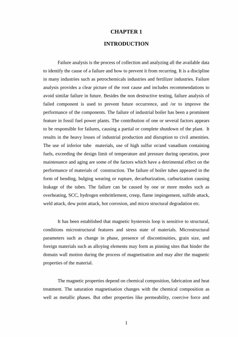
Fig.2. 1. Domain wall dynamics: (a) blowing domain wall motion; (b) rigid

domain wall motion.

There are two main reasons for high-energy storage in domain walls: the one is based

on the Pinning effects of magnetic dipoles and the other on the presence of defects in

the material structure. Since defects can occur in both soft and hard magnetic

materials, it can be said that the blowing process is more likely to occur in low

pinning materials which are the soft magnetic materials, while the parallel motion

occurs in the hard ones. The reversibility of the domain wall propagation defines the

presence or not of hysteresis in the sensing element. Such reversible process depends

mainly on the defects existing in the magnetic substance as well as on the pinning

effect of magnetic dipoles.

2.2.2. Domain rotation dynamics

The domain rotation dynamics have two distinct areas of operation: the irreversible

and the Reversible area of operation. The irreversible rotation occurs when the

magnetic domains, which are oriented on a given easy axis, A, re-orientate to another

easy axis, B, closer to the axis of the external field H, due to the presence of this field

as shown in Fig. 2(a). The reversible domain rotation occurs after the irreversible

rotation process or domain swift. Since the new easy axis B is not in general the same

with the axis of the external field H, the magnetic dipoles tend to orientate to the axis

of the external field H, as shown in Fig. 2(b). After the removal of the external field,

the rotated magnetic domains return back to the easy axis direction B, where they

have been initially and irreversibly re-orientated. In general, magnetic domains do not

return back to their initial easy axis A.

7

Fig. 2.2. Magnetic domain dynamics: (a) two distinct axes of anisotropy and

consequent Irreversible rotation due to the presence of the magnetic field; (b)

reversible magnetic domain rotation after the irreversible magnetization process.

Both reversible and irreversible processes are associated with the presence of

Magnetostriction. The dynamic behavior of these processes can result in elastic

waves, propagating along the magnetic material. The irreversible process is

additionally responsible for the small or large Barkhausen jumps, introducing

magnetic noise in the sensing element. The presence of the irreversible processes in

hysteresis result in magnetic rotation as well as in a relatively higher level of noise

with respect to the reversible processes. Both hysteresis and noise affect the

uncertainty of any possible magnetic device used for sensor application

2.3. Different Models of Hysteresis

2.3.1 Models of hysteresis

Each subject that involves hysteresis has models that are specific to the subject. In

addition, there are models that capture general features of many systems with

hysteresis. An example is the Preisach model of hysteresis, which represents

hysteresis nonlinearity as a linear superposition of square loops called non-ideal

8

relays. Many complex models of hysteresis arise from the simple parallel connection,

or superposition, of elementary carriers of hysteresis termed hysterons.

A simple parametric description of various hysteretic loops may be found in the

Lapshin model of hysteresis. Along with the classical loop, substitution of rectangle,

triangle or trapezoidal pulses instead of the harmonic functions also allows piecewise-

linear hysteresis loops frequently used in discrete automatics to be built in the model

The Bouc–Wen model of hysteresis is often used to describe non-linear hysteretic

systems. It was introduced by Bouc and extended by Wen, who demonstrated its

versatility by producing a variety of hysteretic patterns. This model is able to capture

in analytical form, a range of shapes of hysteretic cycles which match the behavior of

a wide class of hysteretical systems; therefore, given its versability and mathematical

tractability, the Bouc–Wen model has quickly gained popularity and has been

extended and applied to a wide variety of engineering problems, including multi-

degree-of-freedom (MDOF) systems, buildings, frames, bidirectional

and torsional response of hysteretic systems two- and three-dimensional continua,

and soil liquefaction among others. The Bouc–Wen model and its variants/extensions

have been used in applications of structural control, in particular in the modeling of

the behavior of magnetorheological dampers, base isolation devices for buildings and

other kinds of damping devices; it has also been in the modeling and analysis of

structures built of reinforced concrete, steel, masonry and timber

2.3.2 Magnetic hysteresis models

The most known empirical models in hysteresis are Preisach and Jiles-Atherton

models. These models allow an accurate modeling of the hysteresis loop and are

widely used in the industry. However, these models lose the connection with

thermodynamics and the energy consistency is not ensured. Last models rely on a

consistent thermodynamic formulation. VINCH model is inspired by the kinematic

hardening laws and by the thermodynamics of irreversible processes. In particular, in

addition to provide an accurate modeling, the stored magnetic energy and the

dissipated energy are known at all times. The obtained incremental formulation is

variationally consistent, i.e., all internal variables follow from the minimization of a

thermodynamic potential that allows obtaining easily a vectorial model while Preisach

and Jiles-Atherton are fundamentally scalar models.

9

2.4 Magnetic Hysteresis Loop Method as NDE

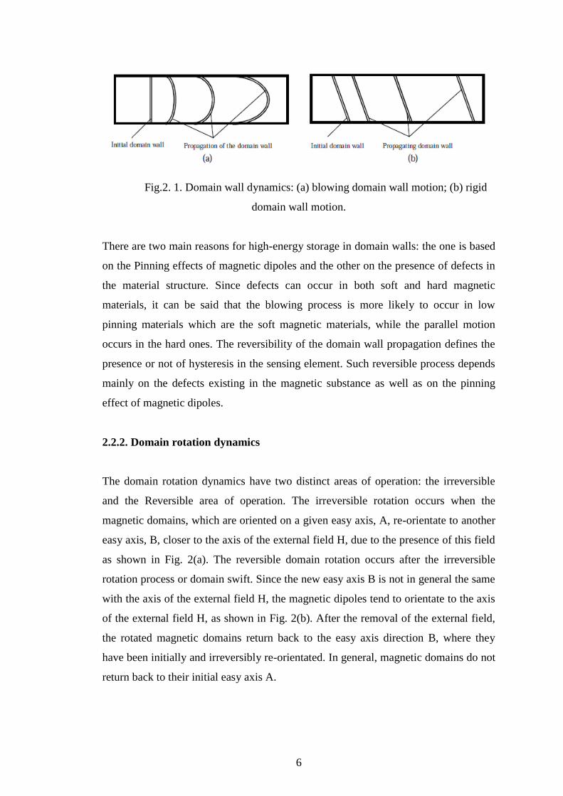
Figure 2.4 is a plot of magnetisation M against applied field H. On application

of a field to a demagnetised sample, M increases with H, reaching the saturation

magnetisation M S if a sufficiently large field is applied. When H is reduced, and

subsequently cycled between positive and negative directions, M follows a hysteresis

loop. A major loop (solid line) is one in which the saturation magnetisation M S of the

material is reached; if this is not the case, the curve is a minor loop (dashed line). The

parameters most commonly used to characterize hysteresis are the field H C required

to reduce M to zero, the value M R of M when H = 0, and the hysteresis energy loss

W H , which is determined from the area enclosed by the loop. H max is the

maximum applied field and H S the field at which M = M S . The positions of greatest

slope change are known as ‘knees’; one of these is marked on Figure 2.4. The slope

dM/dH of the initial magnetisation curve at (H = 0, M = 0) is the initial differential

susceptibility χ0 in, and that of the hysteresis loop at H = H C is the maximum

differential susceptibility χ0 max.

Figure 2.3: A major hysteresis loop (solid line), showing the coercive field HC,

remanence M R and saturation magnetisation M S , and a minor loop (Dashed line).

The arrows show the direction of magnetisation.

10

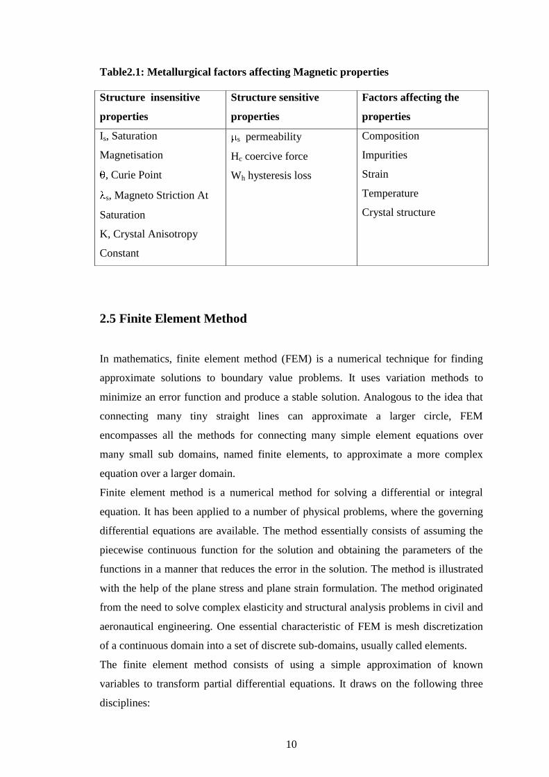
Table2.1: Metallurgical factors affecting Magnetic properties

2.5 Finite Element Method

In mathematics, finite element method (FEM) is a numerical technique for finding

approximate solutions to boundary value problems. It uses variation methods to

minimize an error function and produce a stable solution. Analogous to the idea that

connecting many tiny straight lines can approximate a larger circle, FEM

encompasses all the methods for connecting many simple element equations over

many small sub domains, named finite elements, to approximate a more complex

equation over a larger domain.

Finite element method is a numerical method for solving a differential or integral

equation. It has been applied to a number of physical problems, where the governing

differential equations are available. The method essentially consists of assuming the

piecewise continuous function for the solution and obtaining the parameters of the

functions in a manner that reduces the error in the solution. The method is illustrated

with the help of the plane stress and plane strain formulation. The method originated

from the need to solve complex elasticity and structural analysis problems in civil and

aeronautical engineering. One essential characteristic of FEM is mesh discretization

of a continuous domain into a set of discrete sub-domains, usually called elements.

The finite element method consists of using a simple approximation of known

variables to transform partial differential equations. It draws on the following three

disciplines:

Structure insensitive

properties

Structure sensitive

properties

Factors affecting the

properties

Is, Saturation

Magnetisation

, Curie Point

s, Magneto Striction At

Saturation

K, Crystal Anisotropy

Constant

s permeability

Hc coercive force

Wh hysteresis loss

Composition

Impurities

Strain

Temperature

Crystal structure

11

A feature of FEM is that it is numerically stable, meaning that errors in the input and

intermediate calculations do not accumulate and cause the resulting output to be 10.

2.5.1. JMAG Designer

JMAG is simulation software for the development and design of electrical devices.

JMAG incorporates simulation technology to accurately analyze a wide range of

physical phenomenon that includes complicated geometry, various material

properties, and the heat and structure at the center of electromagnetic fields. JMAG

has an interface capable of linking to third-party software and a portion of the JMAG

analysis functions can also be executed from many of the major Computer Aided

Design (CAD) and Computer Aided Engineering (CAE) systems. JMAG is used

actively to analyze designs at a system level that includes drive circuits by utilizing

links to power electronic simulators. JMAG is also being used for the development of

drive motors for electric vehicles.

JMAG-Designer offers analysis features, link options, and various tools.

Analysis Types

1. Magnetic field analysis

2. Thermal analysis

3. Structural Analysis

4. Electric field analysis

5. Transformer analysis

Magnetic field analysis methods:

Static Analysis:

Static analysis is used when an analysis target does not have time varying phenomena

such as motion and current variations.

Transient Analysis:

12

Transient analysis is used when an analysis target has time varying phenomena such

as motion and current variations.

Frequency Analysis:

Frequency analysis is used when current (or voltage) has sinusoidal variation with

time at the single frequency.

Section analysis:

2D or axis symmetry analyses can be performed using the cross-section of 3D models

like al motor. The section analysis can be used as a preliminary analysis of 3D

analysis.

Section analysis study is created from a 3D analysis study, but the actual analysis is

run with 2D or axis asymmetric model.

2.6. Electro Magnet

An electromagnet is a type of magnet in which the magnetic field is produced

by electric current the magnetic field disappears when the current is turned off.

Electromagnets are widely used as components of other electrical devices, such

as motors, generators, relays, loudspeakers, hard disks, MRI machines, scientific

instruments, and magnetic separation equipment, as well as being employed as

industrial lifting electromagnets for picking up and moving heavy iron objects like

scrap iron.

An electric current flowing in a wire creates a magnetic field around the wire .To

concentrate the magnetic field, in an electromagnet the wire is wound into a coil with

many turns of wire lying side by side. The magnetic field of all the turns of wire

passes through the center of the coil, creating a strong magnetic field there. A coil

forming the shape of a straight tube (a helix) is called a solenoid. Much stronger

magnetic fields can be produced if a "core" of ferromagnetic material, such as

soft iron, is placed inside the coil. The ferromagnetic core increases the magnetic field

to thousands of times the strength of the field of the coil alone, due to the high

magnetic μ of the ferromagnetic material. This is called a ferromagnetic-core or iron-

core electromagnet.

13

The direction of the magnetic field through a coil of wire can be found from a form of

the right hand rule. If the fingers of the right hand are curled around the coil in the

direction of current flow (conventional current, flow of positive charge) through the

windings, the thumb points in the direction of the field inside the coil. The side of the

magnet that the field lines emerge from is defined to be the North Pole.

The main advantage of an electromagnet over a permanent magnet is that the

magnetic field can be rapidly manipulated over a wide range by controlling the

amount of electric current. However, a continuous supply of electrical energy is

required to maintain the field.

2.6.1 How an electro magnet works:

The material of the core of the magnet (usually iron) is composed of small regions

called magnetic domains that act like tiny magnets. Before the current in

Electromagnet is turned on, the domains in the iron core point in random directions,

so their tiny magnetic fields cancel each other out, and the iron has no large scale

magnetic field. When a current is passed through the wire wrapped around the iron, its

magnetic field penetrates the iron, and causes the domains to turn, aligning parallel to

the magnetic field, so their tiny magnetic fields add to the wire's field, creating a large

magnetic field that extends into the space around the magnet. The larger the current

passed through the wire coil, the more the domains align, and the stronger the

magnetic field is. Finally all the domains are lined up, and further increases in current

only cause slight increases in the magnetic field: this phenomenon is called saturation.

When the current in the coil is turned off, most of the domains lose alignment and

return to a random state and the field disappears. However some of the alignment

persists, because the domains have difficulty turning their direction of magnetization,

leaving the core a weak permanent magnet. This phenomenon is called hysteresis and

the remaining magnetic field is called remanent magnetism. The residual

magnetization of the core can be removed by degaussing.

14

2.6.2 Governing equations:

When current flows in a conductor placed in the neighborhood of another

conductor also carrying a current, a force is found to be exerted between them.

Similarly a charge moving in the vicinity of another moving charge is found to

experience a force (over and above the electrostatic force). A magnetic field may be

conceived to be established by one current (or moving charge) and this field then acts

on the second current (or moving charge) in the field. A magnetic induction or field

B is said to exist at a point in space if a conductor carrying a current placed at the

point experiences a force. Experiments show that the force depends on the strength of

the current, the length of the conductor and on the direction of the current. (Note that

B is a vector quantity). We define the direction of the field as that orientation of the

current that experiences zero force, and the magnitude of the magnetic induction B at

a point as the force per unit length acting on a conductor carrying a current of 1

ampere placed Normal to the field. In the special case of a straight wire length ,

placed normal to a homogeneous magnetic field B, the force

F = I B

15

The direction of F being given by the familiar left-hand rule. We can see from the

above equation that the induction B has a dimension of Newton per ampere metre.

A coil of area A and N turns oriented with its plane parallel to a uniform field

B will therefore experience a torque given by NIAB Newton metre.

The magnetic flux through a surface A is defined as the product of the area

of the surface A and the component of the induction B normal to the surface.

= BA cos

Where is the angle between vector B and the normal to the surface. Experiments

show that a changing flux through a circuit induces an e.m.f. equal to the negative rate

of change of flux through the circuit (Faraday's law).

i.e. dt

d

The equation defines the unit of flux, known as the weber. The weber is that change

in flux through a circuit which taking place in 1 second produces an e.m.f. of 1 volt in

the circuit. The equation shows that the weber has the dimension of volt second.

Since = BA, the unit of magnetic induction may be expressed in weber per

square metre.

The unit of B is expressed more commonly in weber/square metre than in

newton per ampere metre. The unit is also called a Tesla.

Note 222

secsec

m

Wb

m

V

mC

mN

mA

N

The magnetic induction B is (from the equation B = /A) a flux density.

16

A useful concept pertaining to the magnetic field B is the concept of lines of

magnetic induction or flux lines. These lines are imagined to fill the space occupied

by the field such that the direction of a line at any point is the direction of the vector B

at the point and such that the concentration of the lines at the point (i.e. the number of

lines per unit area normal to the lines) is set equal to the magnitude of B at the point.

i.e. Bareanormal

linesinductionofnumber

A line of magnetic induction has the dimension of (B x area) and is therefore equal to

one weber.

The magnetic field B which acts on a current or moving charge is set up by

some other current or moving charge. For instance when a current I flows in a long

solenoid, a uniform magnetic field is produced inside the solenoid. This magnetic

field is found to be dependent on the medium in the solenoid, the current I and the

number of turns per metre N

INB

where is a factor dependent on the medium.

IN may be regarded as the cause

which results in the magnetic flux inside the solenoid.

IN is termed the magnetising

force H of the magnetic field (also known as the magnetic field intensity or magnetic

field strength). H is a vector, usually having the same direction as the field B.

Since INH , the unit of H is expressed in ampere-turn per metre (AT/m).

The ratio of the magnetic induction B to the magnetizing force H is called the

absolute permeability or simply the permeability of the medium.

B = H

For free space 0

17

has a dimension: mA

Wb

Am

mWb2

The Weber per ampere meter has the same dimension as Henry per meter (H/m).

A coil carrying a current I1 produces a magnetic field. If another coil of N2

turns is placed in the vicinity of the first coil, a certain amount of the flux will pass

through the second coil, each line of induction linking with N2 turns. The flux linkage

(N2 ) linked with the second coil depends not only on the current I1 but also on the

relative position and geometry of the coils. The relation between and I1 may be

written: 1122 IMN .

M12, the flux linked with one coil when unit current flows in the other, is

known as the Mutual Inductance of the circuits. Further, if the current I1 changes, the

flux linkage N2 also changes and consequently an emf 2 induced in the second

coil.

dt

dIMN

dt

d1222 )(

assuming M12 is independent of the current. This equation is also used to define M12.

The unit of mutual inductance is the Henry. It follows from the definition the Henry

has the dimension:

A

Wb

Ampere

ondvolthenry

sec

A coil in which the current is changing has its changing flux linked with itself so that

a back emf is self induced in the coil:

dt

dIL

L is known as the Self Inductance.

18

2.7 Heat Treatment

2.7.1Normalization

Normalization is the thermal process by which steel is heated into the austenite

phase field—that is, above the Ac 3 for hypo eutectoid (<0.77% carbon) steels and

above the A cm for hypereutectoid (0.77% <carbon <2.1%) steels. Materials are

typically heated to temperatures approximately 100ºF (38ºC) above the upper

temperature and allowed to stabilize so that complete transformation from ferrite to

austenite will occur throughout the thickness of the material. Critical temperatures (A

C1 , A C3, and A CM ) are the temperatures where a material undergoes a phase

change. As steels are heated, they encounter their first critical temperature at

approximately 1350ºF (732ºC), where, depending on composition, the material begins

to transform to austenite. Once uniform temperature is obtained, carbon and other

alloying additions that are soluble in the austenite phase begin to redistribute

themselves throughout the austenitic phase. This homogenization serves to

redistribute the solute elements throughout the matrix to provide a more uniform

dispersion upon cooling than what was imparted during welding and subsequent

solidification.

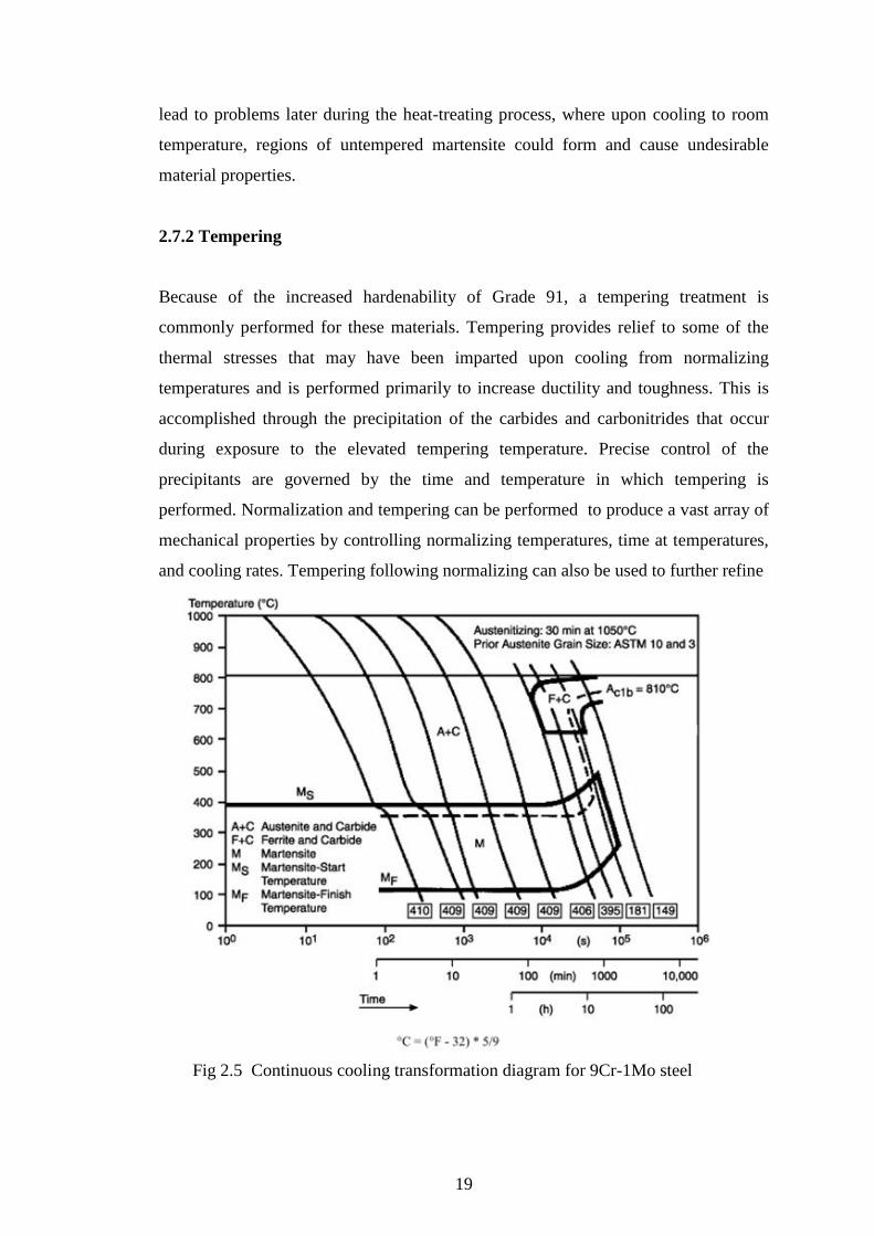
After temperature uniformity has been obtained and sufficient time has been given for

Homogenization to occur, the material is allowed to cool in a uniform manner to room

Temperature. When the material is cooled, it passes two more critical temperatures, m

s and m f. These are the martensite start and martensite finish temperatures, which are

typically represented on a continuous cooling transformation (CCT) diagram, as

shown in Figure

Martensite is formed during non-equilibrium conditions. When an air-hardenable

material such as Grade 91 is heated above the lower critical temperature (A C1) and

allowed sufficient time for partial reaustenitization to occur, transformation to

untempered martensite at the m s temperature is expected. Early results indicate that

the m s is around 400ºF (200ºC) and the m f could be at room temperature or lower.

Another significant aspect of heating above the A C1 temperature is that if a 9CR-

1M0 material is not cooled low enough to completely transform the austenite to

martensite, some retained austenite could remain in the microstructure. This could

19

lead to problems later during the heat-treating process, where upon cooling to room

temperature, regions of untempered martensite could form and cause undesirable

material properties.

2.7.2 Tempering

Because of the increased hardenability of Grade 91, a tempering treatment is

commonly performed for these materials. Tempering provides relief to some of the

thermal stresses that may have been imparted upon cooling from normalizing

temperatures and is performed primarily to increase ductility and toughness. This is

accomplished through the precipitation of the carbides and carbonitrides that occur

during exposure to the elevated tempering temperature. Precise control of the

precipitants are governed by the time and temperature in which tempering is

performed. Normalization and tempering can be performed to produce a vast array of

mechanical properties by controlling normalizing temperatures, time at temperatures,

and cooling rates. Tempering following normalizing can also be used to further refine

Fig 2.5 Continuous cooling transformation diagram for 9Cr-1Mo steel

20

the mechanical properties. Specific procedures must be followed to achieve precise

mechanical properties for the Grade 91 materials. One way to restore properties to

Grade 91 materials that have been heated in the intercritical range is to perform a

normalization heat treatment. This is normally performed at least 100°F (56°C) above

the A C3 temperature and for the material in this project was performed at 1900°F

(1038°C). This results in a fully austenitic microstructure. The material is then air

cooled down to room temperature to transform the austenite to martensite. The

material is now in the condition we want to give us our high-temperature creep

strength, but it is hard and brittle. To gain toughness and soften the metal some, it is

then tempered at 1450°F (788°C).

21

CHAPTER 3

METHODOLOGY

3.1 Simulation with JMAG Software

JMAG is simulation software for the development and design of electrical devices.

JMAG was originally released in 1983 as a tool to support design for devices such as

motors, actuators, circuit components, and antennas.JMAG incorporates simulation

technology to accurately analyze a wide range of physical phenomenon that includes

complicated geometry, various material properties, and the heat and structure at the

center of electromagnetic fields. JMAG has an interface capable of linking to third-

party software and a portion of the JMAG analysis functions can also be executed

from many of the major CAD and CAE systems.

In this work different geometry of the probe are designed and were being analyzed

using JMAG designer software to compare the magnetic fields generated by the probe

and also to optimise the probe parameters such as exciting current and number of

turns for primary and secondary windings. The result shows as follows

Fig: 3.1 JMAG simulation results showing variation of magnetic field and ordered

fashion of magnetic flux lines inside the material

22

Results shows the gradual reduction of magnetic field generated by the probe as the

length between the legs increases from 8 to 32 and it shows higher values for square

probe than that of the curve shaped.

3.2 Experimental Procedure

The core material for the electromagnet of the probe should be of high magnetic

permeability so that it can generate higher magnetic fields. Low carbon steel can

satisfy the above requirement, so horse shoe shaped electromagnets of different

dimensions and geometries are cut from the low carbon steel block. The dimensions

are made in such a way that it can be used to measure the magnetic fields at maximum

number of positions on the failed regions of the tube. Dimensions of the

electromagnet is as

Fig: 3.2Size and geometry of the electromagnet used for the design for the probe

Shown in the fig, two types of geometries were used one with sharp edges and the

other with curved edges. Different dimensions are generated by increasing length

between the two legs of electromagnet from 8mm to 32 mm as 8,16,24,32

respectively. Total 8different electromagnet cores are machined with different

dimensions and geometries.

23

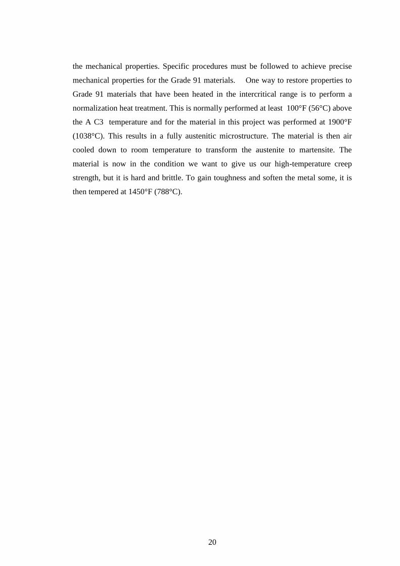
Fig: 3.3Different geometries of probe Fig: 3.4winding of the probe

The magnetic field generated by an electromagnet depends on the number of windings

made over it and the current passes inside the wound coil. More the turns more is the

magnetic field but based on the size of the probe the primary number of turns is

limited to 240 and secondary to 100.for primary winding copper wire with SWG 28

and for secondary winding with copper with SWG 38 is used

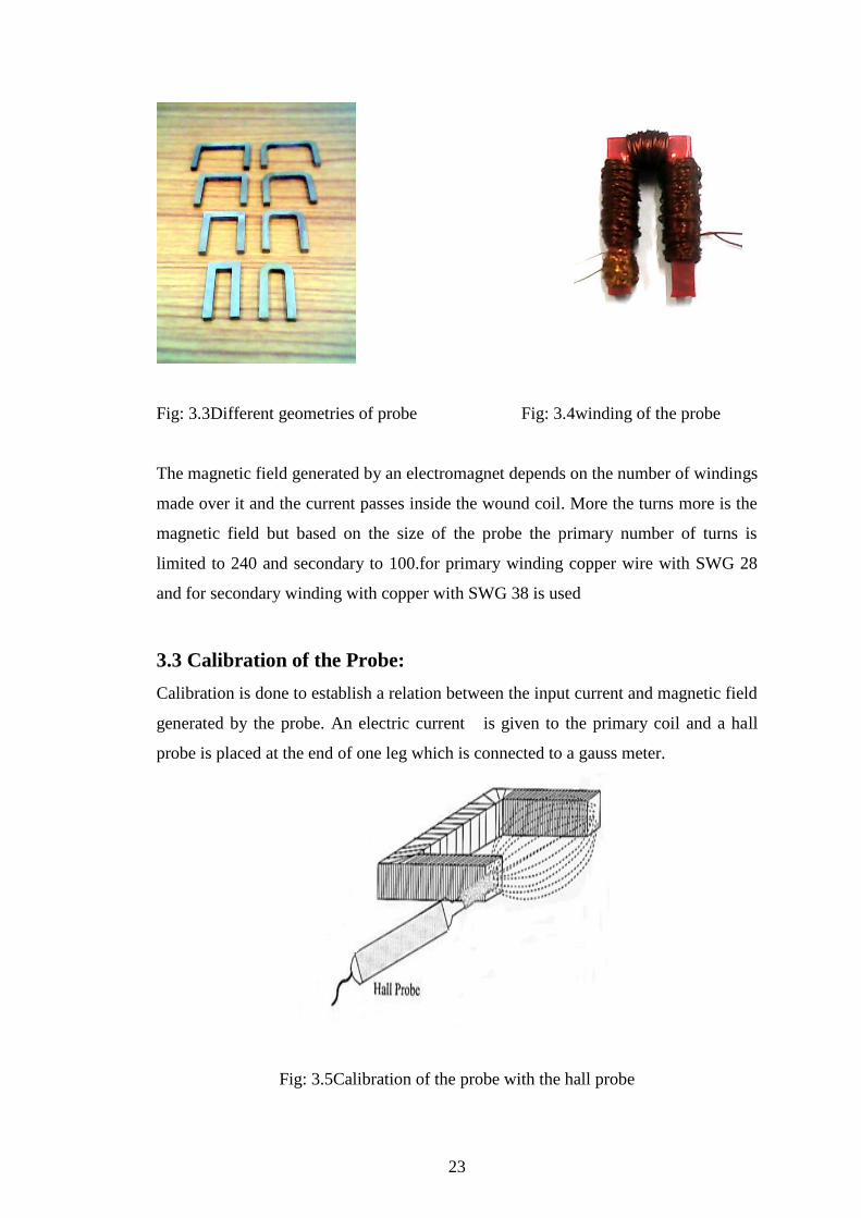
3.3 Calibration of the Probe:

Calibration is done to establish a relation between the input current and magnetic field

generated by the probe. An electric current is given to the primary coil and a hall

probe is placed at the end of one leg which is connected to a gauss meter.

Fig: 3.5Calibration of the probe with the hall probe

24

Fig 3.6 Magnetic field generated by the probe with input current

Gain =

Current is increased slowly from 0 amps to 1.5 amps and slowly reversed the

direction of current from 1.5 amps to -1.5 amps and the corresponding reading in the

gauss meter is noted down at different values of applied current. Magnetic field is

plotted against the applied current. A linear variation of magnetic field with the

current is noticed.

3.4. Inter Facing of the Probe to the Computer

Lab VIEW software was used to interface the probe with the computer as

shown in the fig. A sinusoidal signal from the computer is given to a bipolar amplifier

(kepco: model BOP 80-dM) which amplifies the signal and a sinusoidal electric

current of a required amplitude and very low frequency (50mHz) is fed to the primary

coil which generates a magnetic field and is used to magnetise the test material, low

end of the primary coil is connected to the 1 ohm resistance to monitor the input

current through a multimeter(keithley model:2001) and is fed to the data acquisition

system. Due to change in the flux from the test piece to the core material of the probe

a voltage is generated in the secondary coil which is fed to a flux meter and the data

from the flux meter is given to a data acquisition system (NI Multifunction DAQ).all

-2.0 -1.5 -1.0 -0.5 0.0 0.5 1.0 1.5

-0.6

-0.4

-0.2

0.0

0.2

0.4

0.6

magnetic f

ield

(kgauss)

current (amperes)

Gain:296.4 oesterds/amp

25

the processes including measuring, calculating the properties is done by the Lab

VIEW software installed in the computer.

Fig: 3.7 Block diagram of probe operation

Fig: 3.8 Snap shots of LAB View soft ware while operating with the probe

26

3.5 Study of 9Cr-1Mo Steel Material

3.5.1 Material and Heat treatment

A commercial 9CR-1M0 material of size 5mm thickness, 90mm length and 28 mm

width was used for this study. Composition of 9CR-1M0 material is given by

Table3. 1Chemical composition of 9Cr-1Mo steel material

Name C Si Mn Mo Ni V Cr others Fe

9CR-

1M0

0.08 -

0.12

0.20 -

0.50

0.30 -

.60

0.85

-

1.05

≤0.40 0.18

-

0.25

8.0 -

0.5

Nb_0.06

- 0.10

balance

Samples of 9Cr-1Mo material were studied under different heat treatments.

Initially all the 8 samples were heated to a temperature of 1050o

C and then samples

1,2,3,4 were quenched in water to get a martensite transformation and then samples

5,6,7,8 were normalised (cooled in air) to get a pearlite-ferrite structure. After that

tempering is done for all the samples at different temperatures such as 700,750,770

and 800o C respectively.

Furnace cooling was done for quenched samples and air cooling was done for

normalised samples.

8 samples of above stated size are being heat treated as follows.

Fig: 3.9 block diagram of heat treatment of 9CR-1M0 material

Samples

1,2,3,4 Samples

5,6,7,8

Normalised (air

cooled) at 1050o C

Rapid quenched (water

quenched) at 1050o C

Tempered at

different

temperatures

700,750,770,800o C

for 1Hr

Tempered at

different

temperatures

700,750,770,800o C

for 1Hr

Furnace

cooling

Air

cooling

27

3.5.2. Microstrucural analysis

Micro structure of heat treated samples is analysed with the help of an optical

microscope for the identification of phase and size of grain. Chemical Etching was

done on the specimen by a Villella’s reagent a mixture of 1gram picric acid, 5ml

Hydrochloric acid, 100ml Ethanol as Etchant used for the microstructural evaluation.

3.5.3 Mechanical Property Measurement

Mechanical properties such as hardness values of the tempered samples was

evaluated using Vickers hardness tester of win control UH-3V2.70 the indentation

was made on the cross section of samples under a load of 3 kgf for a time of 10sec

and tensile test was done on a tensile testing machine of model HK25 and Tinius

Olsen Make.

3.5.3 Magnetic Property Measurement

Magnetic measurement was done on the samples with the help of designed probe and

magnetic properties such as coercivity, remanence, and magnetic saturation induction

were evaluated.

28

CHAPTER 4

RESULTS AND DISCUSSION

4.1 Simulation Results

The modeling of electromagnetic probe was done with the help of JMAG software to

optimize the probe parameters such as probe windings, probe geometries and current

etc. It essentially required so that the probe would not be heated up by the eddy

currents generated during operation. The simulated results obtained from modeling

are explained in Fig. 4.1. It is found that 240 turns on the primary coil and 100 turns

on the secondary coil, while the distance between two probe legs is 8mm, can

generate a magnetic field of 290G to magnetize the test material and simultaneously a

signal is received for plotting magnetic induction. The angular edge electromagnets

are capable of generating high magnetic field than that of the curved shaped,

increasing the strength of magnetic field generated with decreasing the distance

between probe legs. The experimental gain is examined with the help of a hall probe

and compared with the simulation gain and the gain reduces with increasing the

length between the horse shoe shaped electromagnet legs.

5 10 15 20 25 30 35

0.022

0.023

0.024

0.025

0.026

0.027

0.028

0.029

0.030

Mag

neti

c f

lux

den

sity

(T)

distance between legs

Experimental

Simulated

Square

5 10 15 20 25 30 35

0.020

0.021

0.022

0.023

0.024

0.025

0.026

0.027

0.028

0.029

Mag

net

ic f

lux

den

sity

(T)

distance between legs

Experimental

Simulated

Curved

Fig 4.1 Magnetic flux density as a function of probe leg length for experimental and

simulated results (a) angular edge probe (b) curved edge probe

29

4.2. Heat Treatment Results

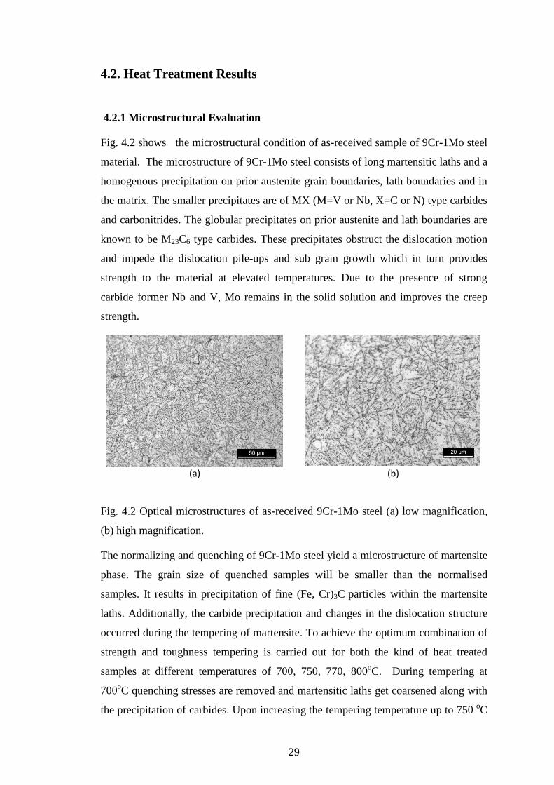
4.2.1 Microstructural Evaluation

Fig. 4.2 shows the microstructural condition of as-received sample of 9Cr-1Mo steel

material. The microstructure of 9Cr-1Mo steel consists of long martensitic laths and a

homogenous precipitation on prior austenite grain boundaries, lath boundaries and in

the matrix. The smaller precipitates are of MX (M=V or Nb, X=C or N) type carbides

and carbonitrides. The globular precipitates on prior austenite and lath boundaries are

known to be M23C6 type carbides. These precipitates obstruct the dislocation motion

and impede the dislocation pile-ups and sub grain growth which in turn provides

strength to the material at elevated temperatures. Due to the presence of strong

carbide former Nb and V, Mo remains in the solid solution and improves the creep

strength.

(a) (b)

Fig. 4.2 Optical microstructures of as-received 9Cr-1Mo steel (a) low magnification,

(b) high magnification.

The normalizing and quenching of 9Cr-1Mo steel yield a microstructure of martensite

phase. The grain size of quenched samples will be smaller than the normalised

samples. It results in precipitation of fine (Fe, Cr)3C particles within the martensite

laths. Additionally, the carbide precipitation and changes in the dislocation structure

occurred during the tempering of martensite. To achieve the optimum combination of

strength and toughness tempering is carried out for both the kind of heat treated

samples at different temperatures of 700, 750, 770, 800oC. During tempering at

700oC quenching stresses are removed and martensitic laths get coarsened along with

the precipitation of carbides. Upon increasing the tempering temperature up to 750 oC

30

this process accelerates and more precipitation occurs at both grain interiors and grain

boundaries. At 750oC, the microstructure comprising homogenous precipitation of

globular M23C6 type carbides become coarse and along with some new phases e.g.

Laves and z phase limits the life of component. The tempering at 770 oC results in the

dissolution of some of the chromium carbides due to the low affinity of chromium

towards carbon compared to other alloying elements present in the material. This

process continues till the tempering below the critical point (AC1) where austenite

phase starts forming. Thus when the tempering temperature is high but below Ac1

number density of M23C6 type carbides reduces and number of MX type precipitates

increases.

A B

C D

31

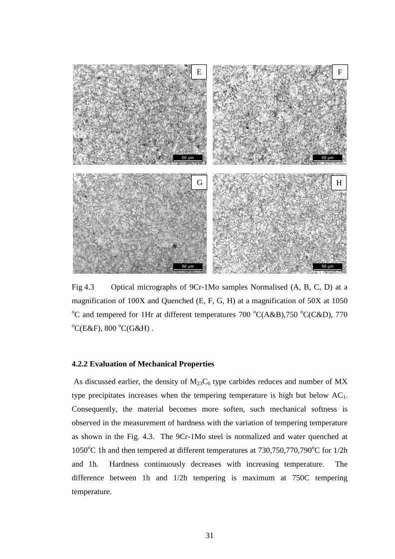
Fig 4.3 Optical micrographs of 9Cr-1Mo samples Normalised (A, B, C, D) at a

magnification of 100X and Quenched (E, F, G, H) at a magnification of 50X at 1050

oC and tempered for 1Hr at different temperatures 700

oC(A&B),750

oC(C&D), 770

oC(E&F), 800

oC(G&H) .

4.2.2 Evaluation of Mechanical Properties

As discussed earlier, the density of M23C6 type carbides reduces and number of MX

type precipitates increases when the tempering temperature is high but below AC1.

Consequently, the material becomes more soften, such mechanical softness is

observed in the measurement of hardness with the variation of tempering temperature

as shown in the Fig. 4.3. The 9Cr-1Mo steel is normalized and water quenched at

1050oC 1h and then tempered at different temperatures at 730,750,770,790

oC for 1/2h

and 1h. Hardness continuously decreases with increasing temperature. The

difference between 1h and 1/2h tempering is maximum at 750C tempering

temperature.

E F

G H

32

730 740 750 760 770 780 790

210

220

230

240

250

260

270

280

290

Har

dnes

s (H

V)

Temperature (oC)

Tempered at 1/2 h

Tempered at 1h

Fig 4.4 variation of hardness with tempering temperature for 1h and ½ h

The tensile test was carried out on the samples tempered at different temperatures

(700,750,770,800) and similar to hardness, the material strength continuously

decreases with increasing tempering temperature (Fig 4.4).

700 720 740 760 780 800

400

500

600

700

800

900

1000

Str

ess

(MP

a)

Temperature

water quenched

Normalised

Yield stress

(a)

33

700 720 740 760 780 800

500

600

700

800

900

1000

1100

1200

Str

ess(

MP

a)

Temperature

water quenched

normalised

Ultimate tensile stress

(b)

Fig 4.5 Tensile test data of 9Cr-1M0 water quenched at 1050C and tempered at

different temperatures (700,750,770,800) respectively (a) yield stress (b) ultimate

tensile stress

4.2.3 Evaluation of Magnetic Properties

Figs. 4.5 to 4.7 show the variation of and coercivity, remanence, and magnetic

saturation induction as a function of tempering temperature. Magnetic properties have

been normalised with respect to normalised and water quenched samples. Both the

normalised and water quenched samples contains martensite phase, therefore the

domain size is very small and the domain wall volume will be large .due to high

dislocation density which acts as pinning site for domain wall, the material becomes

magnetically harder along with high coercivity with progress in tempering

temperature up to 800 oC the effect of precipitation is overwhelmed by the reduction

of dislocation density and removal of quenching stresses. Therefore, material shows a

magnetically softening and hence a decrease in coercivity. This effect can be seen

predominantly in the water quenched samples than that of the normalised samples.

The possible nonmagnetic phase responsible for such behavior present in the alloys is

retained austenite having FCC structure .though the carbides are present, which is

weakly magnetic in nature may not have more impact on the magnetisation. Variation

34

of magnetic saturation values obtained from hysteresis loop measured with the help of

designed probe.

700 720 740 760 780 800

22

23

24

25

26

27

28

29

30

31

32

33

Coer

civit

y(O

e)

Temperature(oC)

Quenched

Normalised

Fig 4.6 variation of Coercivity for normalised and quenched samples

700 720 740 760 780 800

8.6

8.7

8.8

8.9

9.0

9.1

9.2

9.3

9.4

9.5

9.6

Mag

net

ic S

atura

tion I

nduct

ion(K

G)

Temperature(oC)

Quenched

Normalised

Fig 4.7 variation of magnetic saturation induction for normalised and quenched

samples

35

700 720 740 760 780 800

1.6

1.8

2.0

2.2

2.4

2.6

2.8

3.0

Rem

anen

ce(K

G)

Temperature(oC)

Quenched

Normalised

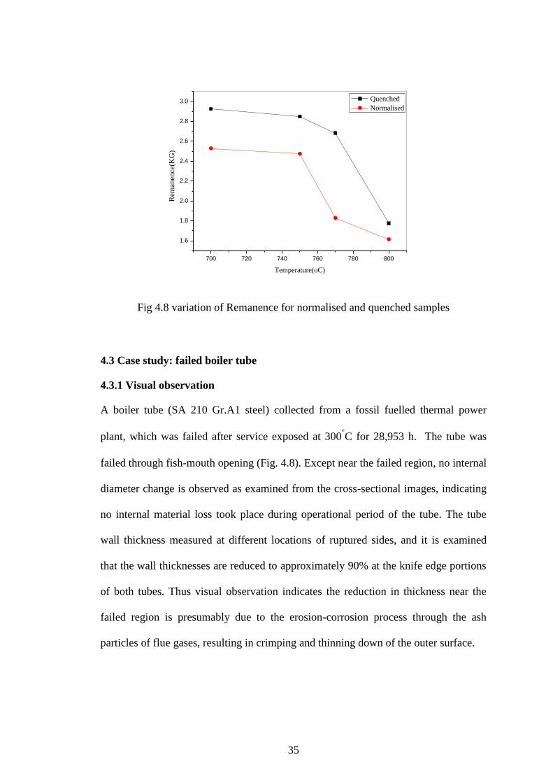
Fig 4.8 variation of Remanence for normalised and quenched samples

4.3 Case study: failed boiler tube

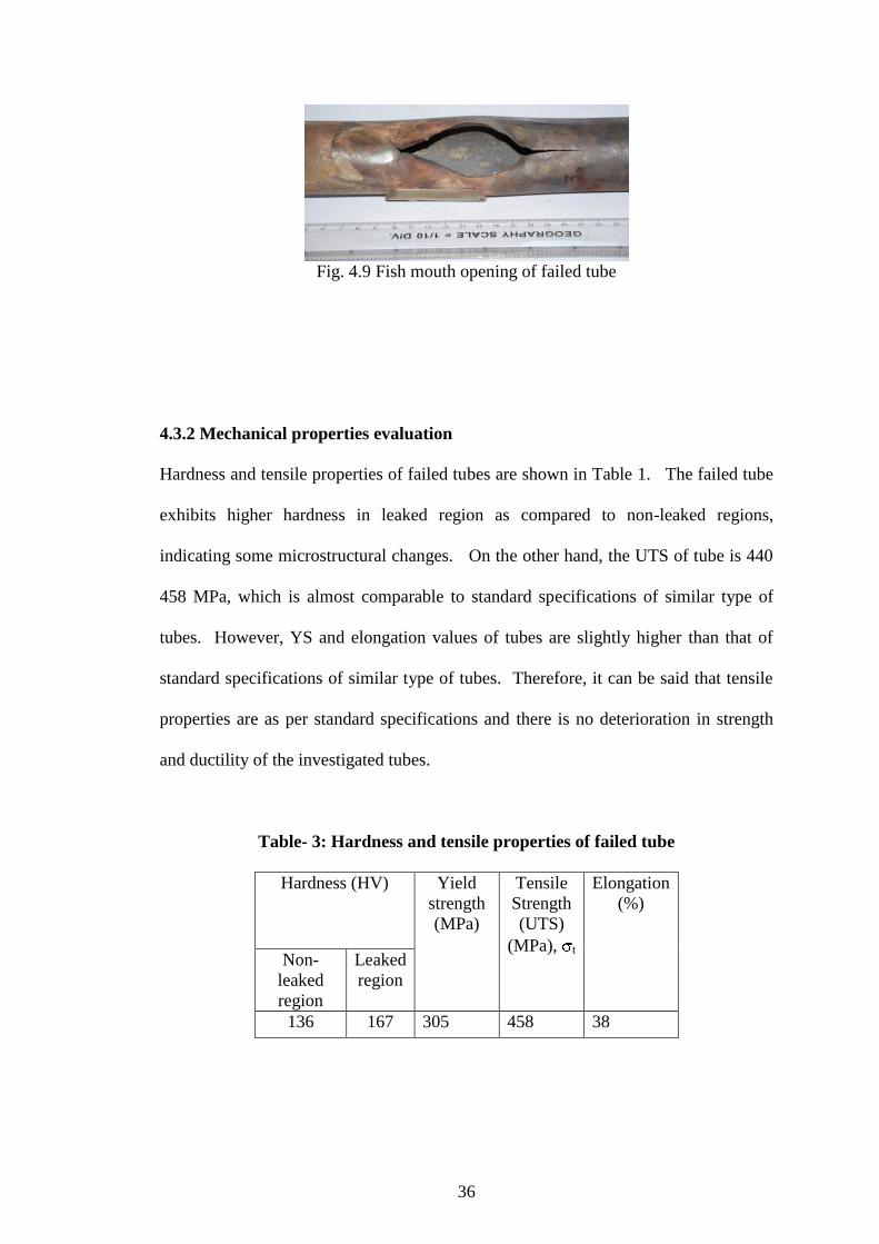
4.3.1 Visual observation

A boiler tube (SA 210 Gr.A1 steel) collected from a fossil fuelled thermal power

plant, which was failed after service exposed at 300 C for 28,953 h. The tube was

failed through fish-mouth opening (Fig. 4.8). Except near the failed region, no internal

diameter change is observed as examined from the cross-sectional images, indicating

no internal material loss took place during operational period of the tube. The tube

wall thickness measured at different locations of ruptured sides, and it is examined

that the wall thicknesses are reduced to approximately 90% at the knife edge portions

of both tubes. Thus visual observation indicates the reduction in thickness near the

failed region is presumably due to the erosion-corrosion process through the ash

particles of flue gases, resulting in crimping and thinning down of the outer surface.

36

Fig. 4.9 Fish mouth opening of failed tube

4.3.2 Mechanical properties evaluation

Hardness and tensile properties of failed tubes are shown in Table 1. The failed tube

exhibits higher hardness in leaked region as compared to non-leaked regions,

indicating some microstructural changes. On the other hand, the UTS of tube is 440

458 MPa, which is almost comparable to standard specifications of similar type of

tubes. However, YS and elongation values of tubes are slightly higher than that of

standard specifications of similar type of tubes. Therefore, it can be said that tensile

properties are as per standard specifications and there is no deterioration in strength

and ductility of the investigated tubes.

Table- 3: Hardness and tensile properties of failed tube

Hardness (HV)

Yield

strength

(MPa)

Tensile

Strength

(UTS)

(MPa), t

Elongation

(%)

Non-

leaked

region

Leaked

region

136 167 305 458 38

37

4.3.3 Microstructure at failed region

Micrographs at the cross-sectional area of the tube near leaked and non-leaked regions

are shown in Fig. 4.9. The tube shows the presence of ferrite and pearlite colonies for

both leaked and non-leaked regions. However, the pearlite colonies are more linked

together at the grain boundary near leaked region, as indicated by arrow in Fig. 4.9b.

The segregation of carbide particles and pearlite colonies near grain boundary might

be related to the crimping and thinning down the outer surface, caused by the

continuous erosion through flue gases and simultaneous coal-ash/fly-ash corrosion .

(a) (b)

Fig.4.10: Optical microstructures of tube showing cross sectional area microstructures

of (a) non-leaked, and (b) leaked regions.

38

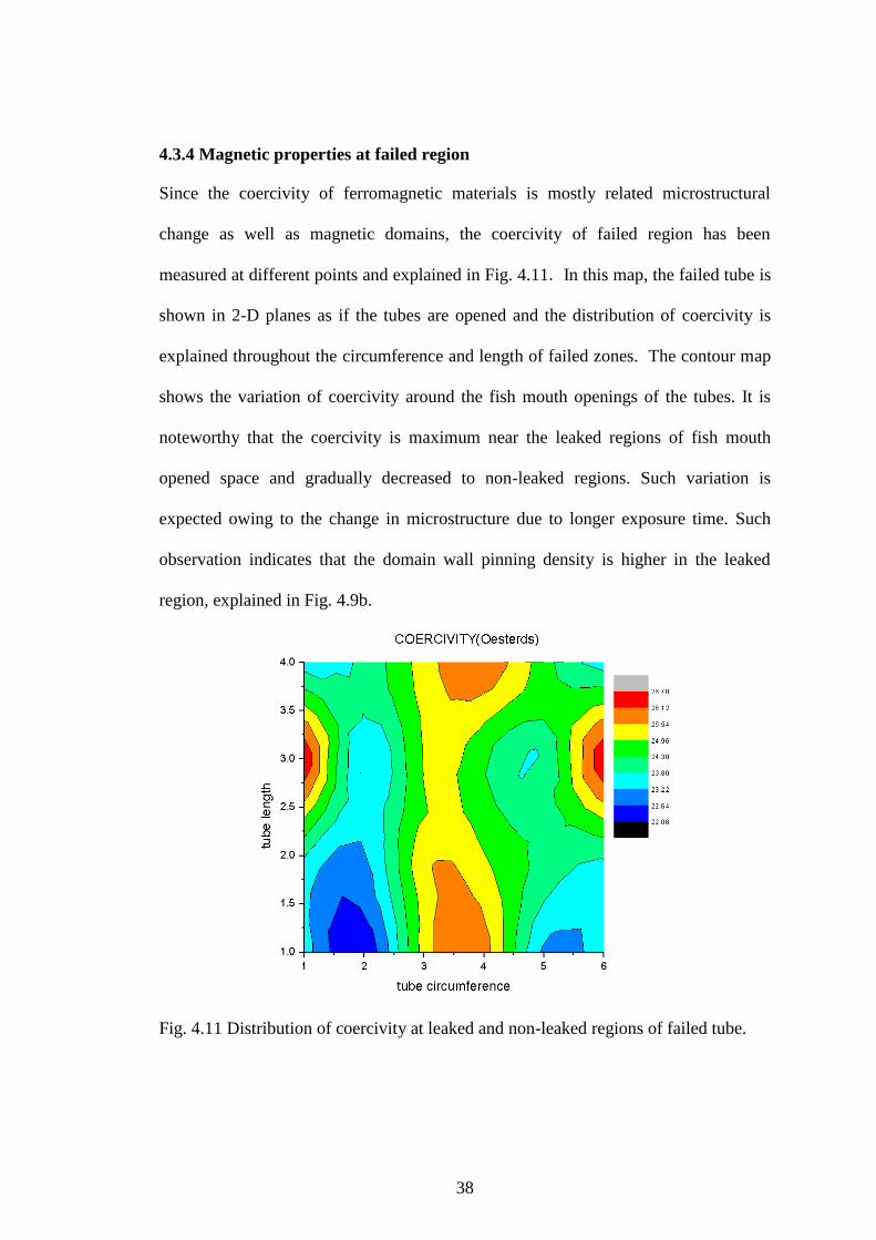
4.3.4 Magnetic properties at failed region

Since the coercivity of ferromagnetic materials is mostly related microstructural

change as well as magnetic domains, the coercivity of failed region has been

measured at different points and explained in Fig. 4.11. In this map, the failed tube is

shown in 2-D planes as if the tubes are opened and the distribution of coercivity is

explained throughout the circumference and length of failed zones. The contour map

shows the variation of coercivity around the fish mouth openings of the tubes. It is

noteworthy that the coercivity is maximum near the leaked regions of fish mouth

opened space and gradually decreased to non-leaked regions. Such variation is

expected owing to the change in microstructure due to longer exposure time. Such

observation indicates that the domain wall pinning density is higher in the leaked

region, explained in Fig. 4.9b.

Fig. 4.11 Distribution of coercivity at leaked and non-leaked regions of failed tube.

39

CHAPTER 5

CONCLUSIONS

5.1 Inferences

1. The present work presents the developing a probe thar is used to generate a

magnetic hysteresis loop and applicability of Magnetic hysteresis loop

technique for material integrity using an electromagnetic probe correlating it

to the microstrucural changes.

2. This method of evaluating the magnetic properties of the material with the

help of electromagnetic techniques will give the material condition and can

avoid the sudden failure of the engineering component in the inservice

inspection.

3. Evaluation of Microstructural changes of components like boiler components

during the service is not possible, so monitoring of magnetic properties during

the inspection may avoid the catastrophic failures.

4. This technique not only depends on the microstructure but also stress state of

the material.

5. Implementation of this technique would help in monitoring as well as

maintaining quality of the material in industrial components that is expected to

get changes in its microstructure and also internal stresses during its service

period.

5.2 Future Work

1. Application of electromagnetic techniques on the welds done on the tubes and flat

plates made up of 9Cr-1Mo steel material.

2. Investigate the variation of magnetic properties in the welds at different heat

treatment processes and to correlate the changes with the microstructures.

40

REFERENCES

1. Magnetism and Metallurgy of Soft Magnetic Materials, Chih-Wen Chen (1977).

2. Investigations On The Failure Of Boiler Tubes In Swcc ,Jeddah Power Plant

,anees U. Malik, nausha asrar, mohammad f. al-ghamdib and Abdullah Hassan

hodhan.

3. Integrated Inspection and Failure Analysis of Boilers, H. A. Abdel-Aleem,

Essam Ibrahim and B. M. Zaghloul.

4. Recent Trends in Electromagnetic NDE Techniques and Future Directions,

B.P.C. Rao, T. Jayakumar, Indira Gandhi Centre for Atomic Research,

Kalpakkam.

5. Influence of microstructural constituents on the hysteresis curves in 0.2%C and

0.45%C steels L F T Costa , F Girotto, R Baiotto, G Gerhardt,M F de Campos,

F P Missell3

6. Magnetic sensing for microstructural assessment of power station steels

assessment: differential permeability and magnetic hysteresis,

iopscience.iop.org.

7. Factors affecting magnetic quality, R.M.Bozoroth.

8. Magnetic effects in physical sensor design and development, E.Hristoforou.

9. Magnetic detection of microstructural changes in power plant steel, Victoria

Anne Yardley, Emmanuel College.