Modeling Survival Using the Kaplan-Meier Estimate Objectives: 1. Simulate the fates of 25 individuals over a 10-day period. 2. Calculate the Kaplan-Meier survival estimate. 3. Graphically analyze the Kaplan-Meier survival curve. 4. Assess how censorship affects the Kaplan-Meier estimate. 5. Determine minimum daily survival rates to ensure population

persistence over time. 6. Learn more about how to use the remarkable functionality of Excel 2013

to plot and analyze wildlife population data. Introduction A population of black bears has been surveyed every 2 years for 20 years and ecologists note that the number of bears in the population has declined over this time frame. Why? Changes in numbers of individuals over time can be directly traced back to the population’s birth, death, immigration, and emigration rates. The population may have declined because the birth rate dropped, the death rate increased, immigration dropped, or emigration increased. Of course, a combination of any or all of these factors may also be responsible for the decline. Mortality and its counterpart, survival, are keys to the population dynamics of all organisms. How do wildlife ecologists estimate these 2 important parameters? In this exercise we’ll explore one method for estimating survival. In Problem set 1, you tracked the fates of individuals over time, noting how many individuals in the cohort were still alive at each time step. You then calculated the survivorship schedule (Sx) and survival probabilities (lx) from your data. Suppose we followed a cohort of 100 radio-tagged, newly-fledged, bobwhite quail over time, carefully noting when deaths occurred. We start with S0 = 100, count individuals again at the next time step (S1) and then at time step S2. Suppose S1 = 40 and S2 = 10. The survivorship schedule tells us the probability that an individual will survive from birth to time x. Thus, the probability of surviving to age 1 is S1/S0 = 40/100 = 0.40, and the probability of surviving from birth to age 2 is S2/S0 = 10/100 = 0.10. Age-specific survival probabilities, in contrast, tell us the probability that an individual will survive from one age to the next—such as the probability that an individual alive in time S1 will be alive at time S2. In life table calculations, the

2

age-specific survival probability is calculated as gx = lx+1/lx. In our example, the probability that an individual bobwhite quail of age S1 will survive to age S2 is 0.10/0.40 = 0.25. The life table “cohort” analysis is one way of calculating survival. However, this method is not always possible to use, especially if the organisms of interest are long-lived. Fortunately, alternatives for estimating survival exist. Kaplan-Meier Survival Analysis When the research question can be posed as “how long does it take until death occurs?” the Kaplan-Meier survival analysis can be used to estimate survival. The Kaplan-Meier method (1958) involves tracking the fates of individuals over time and determining how long it takes for death to occur. In fact, the method has been applied broadly to measure how long it takes for any specific event to occur—such as the time until a cancer patient recovers from a treatment, the time until an infection appears, the time until pollination occurs, and so on. The Kaplan-Meier method is conceptually similar to life table calculations because you keep track of the number of individuals alive and the number of deaths that occur over intervals of time. Specifically, you count the number of individuals who die at a certain time and divide that number by the number of individuals that are “at risk” (alive and part of the study) at that time. If we do this for each time period in the study, we will be able to compute 2 survival probabilities: the conditional survival probability (Pc) and the unconditional survival probability (Pu). We will describe how each is computed with a brief example. Let’s say you conducted a radio-telemetry study of the weekly survival of yearling male white-tailed deer by tracking 50 individuals from fixed-wing aircraft for a 1 year. Once per week you recorded the number of deaths and the number of individuals still alive. Let’s also suppose that some yearlings in your study population emigrated out of the population so you can no longer track their fates. The data you collected during the first 5 weeks of the study are located in Table 1.

3

Table 1. Weekly conditional survival probabilities (Pc) for a hypothetical yearling male white-tailed deer population. Week

(t) No.

Emigrants No.

Deaths (d)

No. at risk (n)

Deaths/no. at risk

Pc

1 1 1 50 1/50 = 0.02 1 – 0.02 = 0.98 2 0 1 50 – 1 – 1 = 48 1/48 = 0.02 1 – 0.02 = 0.98 3 0 0 48 – 1 = 47 0/47 = 0 1 – 0 = 1.00 4 0 0 47 – 0 = 47 0/47 = 0 1 – 0 = 1.00 5 0 0 47 – 0 = 47 0/47 = 0 1 – 0 = 1.00

Now let

t = a particular time period, such as 1 week, d = the number of deaths at time ti, and n = the number of individuals at risk at the beginning of time ti.

The conditional survival probability, Pc, is the probability of surviving to a specific time, given that you survived to the previous time (this is similar to the age-specific survival probabilities in the life table). Pc is computed as

𝑃𝑃𝑐𝑐 = 1 −𝑑𝑑𝑖𝑖𝑛𝑛𝑖𝑖

.

The term di/ni gives the number of individuals that die in time step i divided by the number of individuals still alive and still in the population (the number at risk). This is the conditional mortality probability, or the probability that an individual will die during that time step. Since survival can be computed as 1 minus mortality, Equation 1 gives Pc. Because you started with a population of 50 individuals, the number at risk for death at the beginning of week 1 is 50. During that week, 1 individual died, so the conditional mortality probability is 1/50 = 0.02, and the conditional survival probability is 1 – 0.02 = 0.98. Now let’s consider week 2. At the beginning of week 2, there are 49 individuals at risk. One individual died the previous time step, and one left the population through emigration. The individual that left the study is called a censored observation.

4

Individuals that die in the previous time step, as well as censored individuals, cannot be considered at risk, so at the beginning of week 2 48 individuals are at risk. During week 2, 1 death occurred, so the conditional mortality probability is 1/48 = 0.02, and Pc = 1 – 0.02 = 0.98. The Pc calculations for the duration of the study are shown in Appendix A. The unconditional survival probability, Pu, is the probability of survival from the start of the study to a specific time (this is similar to the survivorship schedule in the life table). Pu equals the cumulative product of the conditional probabilities, which is why the Kaplan-Meier method is sometimes called the Kaplan-Meier product limit estimate. The equation can be expressed as:

𝑃𝑃𝑢𝑢 = ��1 −𝑑𝑑𝑗𝑗𝑛𝑛𝑗𝑗�

𝑖𝑖

𝑗𝑗=1

,

where the Π symbol means “multiply all of the individual conditional probabilities together.” Pu is calculated through week 5 in Table 2. The calculations for the duration of the study are shown in Appendix A. Table 2. Weekly conditional (Pc) and unconditional survival probabilities (Pu) for a hypothetical yearling male white-tailed deer population. Week

(t) No.

Emigrants No.

Deaths (d)

No. at risk (n)

Deaths/no. at risk

Pc Pu

1 1 1 50 1/50 = 0.02 1 – 0.02 = 0.98 0.98 2 0 1 50 – 1 – 1 = 48 1/48 = 0.02 1 – 0.02 = 0.98 0.98 * 0.98 = 0.96 3 0 0 48 – 1 = 47 0/47 = 0 1 – 0 = 1.00 0.98 * 0.98 * 1 = 0.96 4 0 0 47 – 0 = 47 0/47 = 0 1 – 0 = 1.00 0.98 * 0.98 * 1 * 1 = 0.96 5 0 0 47 – 0 = 47 0/47 = 0 1 – 0 = 1.00 0.98 * 0.98 * 1 * 1 * 1 = 0.96

For week 1, Pu is the same as Pc. Pu for week 2 gives the probability that an individual at the start of the study will survive through week 2. This is obtained by multiplying the Pc for week 1 by the Pc for week 2, since both conditions must be met in order for an individual to be alive at the end of week 2. Got it?

5

Kaplan-Meier Survival Curves The results of the Kaplan-Meier analysis are often graphed. Such graphs are known as the Kaplan-Meier survival curves (Figure 3). Comparing the survival curves of 2 different populations, age classes within a population, or by gender can yield insightful information about the timing of deaths in response to different environmental conditions.

Figure 3. Kaplan-Meier survival curves for a hypothetical yearling white-tailed deer population. The unit time is plotted on the x-axis; Pu is plotted on the y-axis. In Kaplan-Meier curves, the raw data are plotted as in graph a, then the data points are connected with horizontal and vertical bars as in graph b. Large vertical steps downward (as within weeks 20-25) indicate a relatively large number of deaths in the given time period, while large horizontal steps (as within weeks 5-20 and 25-50) indicate few deaths during a time interval. The Pu data plotted here are located in Appendix A. Procedures The method outlined by Kaplan and Meier (1958) to estimate survival is one of the most referenced papers in science, suggesting that is has played an important role in wildlife ecology and other sciences since its publication. The goal of this problem set is to create a spreadsheet model of the Kaplan-Meier method and use the model to (1) learn how censored observations affect survival probabilities, and (2) determine the minimum daily survival rate required to ensure that a population will persist for a specified time period.

Week

0 5 10 15 20 25 30 35 40 45 50 55

Unco

ndit

iona

l sur

viva

l rat

e (P

u)

0.60

0.65

0.70

0.75

0.80

0.85

0.90

0.95

1.00

Week

0 5 10 15 20 25 30 35 40 45 50 55

Unco

ndit

iona

l sur

viva

l rat

e (P

u)

0.60

0.65

0.70

0.75

0.80

0.85

0.90

0.95

1.00

a b

6

A. Set up the model population 1. Open a new spreadsheet and set up column headings as shown in Figure

4. We’ll track 25 individuals for 10 days and keep track of their fates over time. Such a short time frame would perhaps be most relevant for a larval invertebrate population. Row 10 will track individual 1’s fate, row 11 will track individual 2’s fate, and so on to row 34.

2. Set up a linear series from 1 to 25 in cells A10–A34. In cell A10 enter the value 1. In cell A11 enter the formula =1+A10. Copy this formula down to cell A34.

Figure 4

3. In cell B4, enter a value for the probability that an individual will survive each 24-hour period (daily survival). Enter the value 0.9 in cell B4. In reality, you wouldn’t know what this number is; you are using the Kaplan-Meier method to estimate this parameter.

4. In cell B5, enter the value 25, which is the number of individuals in the initial population.

5. In cells B6–K6, enter a value for the probability that an individual in the population will be censored on a given day. Enter the value 0.1 in cells B6–K6. This is the probability that an individual will leave the study on any given day so that its fate cannot be tracked over time. For now, we set that probability to 0.1 for all days. Later in the exercise you will change these values to determine how censored observations, and the time at which they occur, affect survival probability estimates. At this point, your spreadsheet should look like Figure 5.

7

Figure 5

B. Simulate fates of individuals over time

1. In cells B10–B34, enter a formula to assign a fate to each individual for day 1. In the real world, your research would supply these data. Here, the fate data are being simulated. In cell B10 enter the formula =IF(RAND()<$B$6,"C",IF(RAND()>$B$4,"D",1)). Copy your formula down to row 34. The formula in B10 will assign a fate to individual 1 on day 1. The individual will be either alive (1), censored (C), or dead (D). The formula contains 2 IF functions and a RAND (random) function, so it is a nested formula. Remember that the IF function consists of 3 parts separated by commas. In the first part of the function, you specify a criterion. If the criterion is true, the spreadsheet will do or carry out

8

whatever you specify in the second portion of the function. If the criterion is false, the spreadsheet will carry out what you specify in the third portion of the function. Let’s review the B10 formula carefully.

The criterion is that a random number (the RAND() portion of the formula) is less than the value in cell B6 (the probability of being censored on day 1). If the criterion is true, the individual is censored and the spreadsheet will return the letter C. If the criterion is false, the individual is not censored, and the second IF function will be computed. The second IF function tells the spreadsheet to evaluate whether a random number between 0 and 1 is greater than the value in cell B4—the true (but unknown to you, the researcher) daily survival probability. If the random number is greater than the survival probability, the individual will die (the spreadsheet will return the letter D). If the random number is less than the value in cell B4, the spreadsheet will return the number 1, indicating that the individual survived that day. When you copy your formula down for the 25 individuals in the population, you should see that some individuals die and some become censored. Press F9, the calculate key, to randomly generate new fates for individuals in the population. Typing into cells will also generate new values. Don’t forget that one of the objectives of this problem set is to learn more about how to use the remarkable functionality of Excel 2013 to plot and analyze wildlife population data. The use of nested formulas and IF, OR, and RAND functions are advanced uses of spreadsheets. No other course in the wildlife curriculum at UAM provides you with the opportunity to use some of the advanced features in Excel 2013. You are introduced to them here because you will have use for them as a wildlife professional.

2. In cell C10, enter a formula to assign a fate to individual 1 for day 2. In

cell C10 enter the formula =IF(OR(B10="D",B10="C",B10=""),"",IF(RAND()<$C$6,"C",IF(RAND()>$B$4,"D",1))). Don’t be intimidated by the length and complexity of this formula. If the individual in cell C10 died or was censored on day 1, we want to return

9

a blank cell (i.e., that is what the 2 double quotes will do). If the individual survived day 1, then we want to know what happened on day 2. The formula in cell C10 is another nested IF function. There are multiple criteria, however, in the first IF function, and these criteria are given with an OR function. The OR function is used to evaluate whether the value in cell B10 is “D” or “C” or “”. If any one of those 3 conditions is true, the spreadsheet will return a blank, or “”. If none of the conditions is true, the individual must have survived day 1, and the second IF function is computed; it has the same form as the formula in cell B10, with the spreadsheet again returning a value of “C,” “D,” or the number 1.

3. Select cell C10, and copy its formula across to cell K10. Modify the

formula in each cell to reflect the probability of censorship for the appropriate day. Be careful here; it is easy to make mistakes. Double-check your formulas and make sure they are entered correctly. Your formulas should read as follows:

In cell D10, =IF(OR(C10="D",C10="C",C10=""),"",IF(RAND()<$D$6,"C",IF(RAND()>$B$4,"D",1))) In cell E10, =IF(OR(D10="D",D10="C",D10=""),"",IF(RAND()<$E$6,"C",IF(RAND()>$B$4,"D",1))) In cell F10, =IF(OR(E10="D",E10="C",E10=""),"",IF(RAND()<$F$6, "C",IF(RAND()>$B$4, "D",1))) In cell G10, =IF(OR(F10="D",F10="C",F10=""),"",IF(RAND()<$G$6, "C",IF(RAND()>$B$4, "D",1))) In cell H10, =IF(OR(G10="D",G10="C",G10=""),"",IF(RAND()<$H$6,"C",IF(RAND()>$B$4, "D",1)))

10

In cell I10, =IF(OR(H10="D",H10="C",H10=""),"",IF(RAND()<$I$6,"C",IF(RAND()>$B$4, "D",1))) In cell J10, =IF(OR(I10="D",I10="C",I10=""),"",IF(RAND()<$J$6, "C",IF(RAND()>$B$4, "D",1))) In cell K10, =IF(OR(J10="D",J10="C",J10=""),"",IF(RAND()<$K$6,"C",IF(RAND()>$B$4,"D",1)))

4. Select cells C10–K10, and copy the formula down to row 34. Your spreadsheet should now resemble Figure 6, although the fates of your individuals will likely be different than that shown because the fates are randomly determined.

Figure 6

11

C. Compute survival probabilities

The first calculations in the Kaplan-Meier estimate involve counting the number of individuals at risk (those still alive) during each day, and to count the number of deaths that occur each day.

1. In cell A35 set up new headings as shown in Figure 7. Notice that

whenever a new formula or text is entered, the simulated fates change.

Figure 7

2. In cell B35, enter 25, the number of at-risk individuals in the population

on day 1. The number at risk on day 1 is 25 because we started with a sample size of 25.

3. In cell B36, enter a formula to count the number of deaths on day 1. In cell B36 enter the formula =COUNTIF(B10:B34, "D"). The number of deaths on day 1 is the number of D’s that appear for the 25 individuals.

4. In cell B37, enter a formula to count the number of censored observations on day 1. In cell B37 enter the formula =COUNTIF(B10:B34, "C"). The number of censored observations on day 1 is the number of C’s that appear for the 25 individuals.

5. In cell B38, enter a formula to compute Pc. In cell B38, enter the formula =1-(B36/B35). This is the spreadsheet version of the equation on page 3.

12

Remember, Pc is the probability of survival to a particular time period, given that you survived to the previous time. This probability is easy to calculate if you know the number of deaths at a specific time and the number of individuals at risk at that same time. The number of deaths divided by the number at risk gives the conditional probability of mortality, so 1 minus that value is Pc.

6. In cell B39, enter a formula to compute Pu. In cell B39 enter the formula =PRODUCT($B$38:B38). Pu is the probability of surviving to a particular time. It is calculated in the equation on page 4 as the cumulative product of the conditional probabilities.

7. In cell B40, enter a formula to compute the expected Pu for day 1, given the survival parameter in cell B4. In cell B40 enter the formula =$B$4^B9. The ^ symbol means raise the value in cell B4 (the survival probability) to the number of days under consideration.

8. In cell B41, enter the formula to compute the actual daily survival for each Pc. In cell B41 enter the formula =B39^(1/B9) to obtain the daily survival estimate for day 1. Remember that the Pc gives the probability of surviving to a specific time period. To convert the Pc to daily survival probabilities, take the appropriate root. For example, take the third root of Pc for day 3, the seventh root of Pc for day 7, and so on, to obtain the daily survival estimate. To obtain roots in spreadsheets, use the exponent form (^) with the exponent as a fraction (i.e., ^(1/B9)).

9. In cell C35, compute the number of individuals at risk for day 2. In cell C35 enter the formula =B35-(B36+B37). Remember that the number of individuals at risk are those currently alive and not censored.

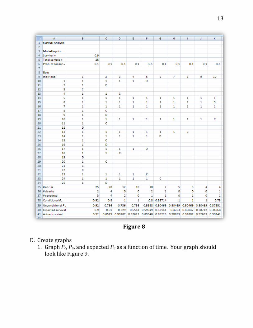
10. Select the formulas from steps 3–8 and copy them across to column K. Your spreadsheet should now look like Figure 8, but (with the exception of Row 40) your numbers will likely be different.

13

Figure 8

D. Create graphs

1. Graph Pc, Pu, and expected Pu as a function of time. Your graph should look like Figure 9.

14

Figure 9

Your graph will look different than the Kaplan-Meier survival curve in Figure 3b because the points are connected differently. However, Figures 3b and 9 are interpreted the same way. Note that the expected Pu is virtually a straight line because we set the daily survival probability as a constant over time. Sharp drops in the Pu line indicate more mortality on a given day, and shallow drops in a line indicate fewer deaths. Figure 9 shows no deaths occurred from Day 8 to Day 10. Your results may vary.

2. Press F9 to generate a new simulation. How do your results appear to

change with each new simulation? Your results should vary from simulation to simulation. This is due to the random number function changing the data set, and it is also due to the fact that our population consists of only 25 individuals, so there is some demographic stochasticity in this model. (We will talk about demographic stochasticity in class.) In order to better understand how Pc and Pu “behave” over the 10-day period, we need to run several simulations, and track our results. We will do that in the next step.

0.3

0.4

0.5

0.6

0.7

0.8

0.9

1

1 2 3 4 5 6 7 8 9 10

Prob

abili

ty o

f sur

viva

l

Day

Conditional Pc

Unconditional Pu

Expected survival

15

E. Track 100 simulations 1. Set up new headings in your spreadsheet as shown in Figure 10, but

extend the trials to 100 (cell M109) and the days to 10 (cell W9).

Figure 10

2. Record a macro to track Pu for 100 trials, logging your results in cells

N10–W109. To open the macro function select Developer | Record Macro. Once you have assigned a Macro name, click OK. The macro is now in record mode. Perform the following steps: • Select cells B39–K39. Copy. • Select cell N9. Select Home | Find & Select | Find. These steps will

open the “Find and Replace” dialog box. Leave the “Find What” box empty. Click on the options >> button and “Search By Columns”. Select Find Next, then Close. Your cursor should move down to cell N10.

• Right click on cell N10. Select Paste Special | Paste Values | Values. • Select Developer | Stop Recording. • Run your macro until 100 trials have been computed.

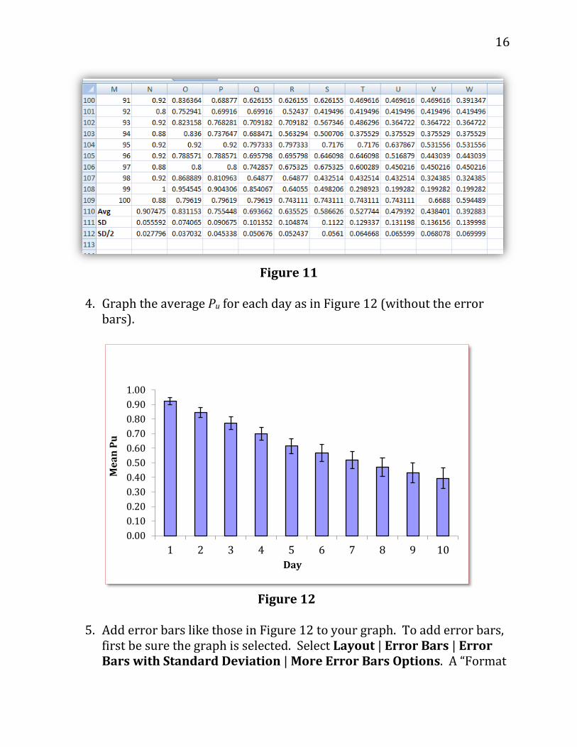
3. Use the AVERAGE function in cells N110–W110 and STDEV function in cells N111–W111 to compute the average Pu and standard deviation (SD) for the 100 trials. Your formula for day 1 should be =AVERAGE(N10:N109). This gives the average unconditional probability that an individual will survive past day 1. The SD is computed as =STDEV(N10:N109). Also divide each SD by 2 in cells N112–W112. You will want to divide this number by 2 for graphing purposes in the next step. See Figure 11.

16

Figure 11

4. Graph the average Pu for each day as in Figure 12 (without the error

bars).

Figure 12

5. Add error bars like those in Figure 12 to your graph. To add error bars,

first be sure the graph is selected. Select Layout | Error Bars | Error Bars with Standard Deviation | More Error Bars Options. A “Format

0.000.100.200.300.400.500.600.700.800.901.00

1 2 3 4 5 6 7 8 9 10

Mea

n Pu

Day

17

Error Bars” dialog box appears (Figure 13). Click Display Both and Custom. When you click the Specify Value button a second, smaller “Custom Error Bars” dialog box appears (Figure 13). Place your cursor in the box labeled “Positive Error Value,” then use your mouse to select the standard deviations for your 100 trials divided by 2 (cells N112–W112). Do the same for the box labeled “Negative Error Value.” Click OK and then Close. Your graph should be updated and look like Figure 12.

Figure 13 Discussion Questions 1. Interpret the Pc and Pu curves in Figure 9. What do long stretches of

slightly sloping or horizontal lines indicate? What do steeply sloping vertical drops indicate?

2. Although all wildlife populations, of course, must maintain some minimum rate of survival to persist through time, the issue is especially important in small T&E populations. What level of daily survival is needed to ensure that the population we created in this exercise will persist for 10 days? Set up your spreadsheet as shown below. Enter the expected Pu’s for each level of daily survival (given in cells A45–A53). For example, cell B45

18

should compute Pu for day 1 when the daily survival is 0.1. Graph your results. What does the minimum Pu have to be for the population to persist for at least 10 days? If we started with a population larger than 25, say 500 individuals, do you think your results would be different? How would you test that question?

3. The Kaplan-Meier estimate is used to estimate survival because

“uncooperative” individuals can be taken out of the picture. For example, individuals that emigrate out of your study area are censored observations and can be subtracted from your “at risk” population. Compare your model results to a population where censored observations are absent (cells B6–K6 = 0). Erase your macro results (cells N10–W109), then run your macro again under the new conditions. Compare the mean Pu and the standard deviations of the trials. You can do that by creating another graph like Figure 12.

4. What do the error bars in Figure 12 tell you about the mean daily Pu values?

5. By week 52 in the hypothetical yearling male white-tailed deer population in Appendix A, the Pc value was 1.00 and the Pu value was 0.66. Explain what these numbers mean to a member of the general public who is not trained in wildlife population ecology.

Literature Cited Kaplan, E. L. and P. Meier. 1958. Nonparametric estimation from incomplete observations. Journal of the American Statistics Association 53: 457–481.

19

Acknowledgement This problem set was adapted from Exercise 24: Survival analysis, pages 311-320 in Donovan, T. M. and C. Welden. 2002. Spreadsheet exercises in ecology and evolution. Sinauer Associates, Inc. Sunderland, MA, USA. This publication is at http://www.uvm.edu/rsenr/vtcfwru/spreadsheets/?Page=ecologyevolution/EE24.htm. Your write-up should include the following: (1) a paragraph explaining the objectives of this problem set, and (2) your answers to the 5 discussion questions above. Email me (whited@uamont.edu) your Kaplan-Meier spreadsheet model.

Week Emigrants Deaths No. at risk Deaths/at risk Pc Pu1 1 1 50 1/50 = 0.02 1 - 0.02 = 0.98 0.982 0 1 50 - 1 - 1 = 48 1/48 = 0.02 1 - 0.02 = 0.98 0.98 * 0.98 = 0.963 0 0 48 - 1 = 47 0/47 = 0 1 - 0 = 1.00 0.98 * 0.98 * 1 = 0.964 0 0 47 - 0 = 47 0/47 = 0 1 - 0 = 1.00 0.98 * 0.98 * 1 * 1 = 0.965 0 0 47 - 0 = 47 0/47 = 0 1 - 0 = 1.00 0.98 * 0.98 * 1 * 1 * 1 = 0.966 0 0 47 - 0 = 47 0/47 = 0 1 - 0 = 1.00 0.98 * 0.98 * 1 * 1 * 1 * 1 = 0.967 1 0 47 - 0 = 47 0/47 = 0 1 - 0 = 1.00 0.98 * 0.98 * 1 * 1 * 1 * 1 * 1 = 0.968 0 1 47 - 1 = 46 1/46 = 0.02 1 - 0.02 = 0.98 0.98 * 0.98 * 1 * 1 * 1 * 1 * 1 * 0.98 = 0.949 0 0 46 - 1 = 45 0/45 = 0 1 - 0 = 1.00 0.98 * 0.98 * 1 * 1 * 1 * 1 * 1 * 0.98 * 1 = 0.94

10 0 0 45 - 0 = 45 0/45 = 0 1 - 0 = 1.00 0.98 * 0.98 * 1 * 1 * 1 * 1 * 1 * 0.98 * 1 * 1 = 0.9411 0 0 45 - 0 = 45 0/45 = 0 1 - 0 = 1.00 0.98 * 0.98 * 1 * 1 * 1 * 1 * 1 * 0.98 * 1 * 1 * 1 = 0.9412 0 0 45 - 0 = 45 0/45 = 0 1 - 0 = 1.00 0.98 * 0.98 * 1 * 1 * 1 * 1 * 1 * 0.98 * 1 * 1 * 1 * 1 = 0.9413 0 0 45 - 0 = 45 0/45 = 0 1 - 0 = 1.00 0.98 * 0.98 * 1 * 1 * 1 * 1 * 1 * 0.98 * 1 * 1 * 1 * 1 * 1 = 0.9414 0 0 45 - 0 = 45 0/45 = 0 1 - 0 = 1.00 0.98 * 0.98 * 1 * 1 * 1 * 1 * 1 * 0.98 * 1 * 1 * 1 * 1 * 1 * 1 = 0.9415 0 0 45 - 0 = 45 0/45 = 0 1 - 0 = 1.00 0.98 * 0.98 * 1 * 1 * 1 * 1 * 1 * 0.98 * 1 * 1 * 1 * 1 * 1 * 1 * 1 = 0.9416 0 0 45 - 0 = 45 0/45 = 0 1 - 0 = 1.00 0.98 * 0.98 * 1 * 1 * 1 * 1 * 1 * 0.98 * 1 * 1 * 1 * 1 * 1 * 1 * 1 * 1 = 0.9417 0 0 45 - 0 = 45 0/45 = 0 1 - 0 = 1.00 0.98 * 0.98 * 1 * 1 * 1 * 1 * 1 * 0.98 * 1 * 1 * 1 * 1 * 1 * 1 * 1 * 1 * 1 = 0.9418 0 0 45 - 0 = 45 0/45 = 0 1 - 0 = 1.00 0.98 * 0.98 * 1 * 1 * 1 * 1 * 1 * 0.98 * 1 * 1 * 1 * 1 * 1 * 1 * 1 * 1 * 1 * 1 = 0.9419 1 0 45 - 0 = 45 0/45 = 0 1 - 0 = 1.00 0.98 * 0.98 * 1 * 1 * 1 * 1 * 1 * 0.98 * 1 * 1 * 1 * 1 * 1 * 1 * 1 * 1 * 1 * 1 * 1 = 0.9420 0 0 45 - 1 = 44 0/44 = 0 1 - 0 = 1.00 0.98 * 0.98 * 1 * 1 * 1 * 1 * 1 * 0.98 * 1 * 1 * 1 * 1 * 1 * 1 * 1 * 1 * 1 * 1 * 1 * 1 = 0.9421 0 0 44 - 0 = 44 0/44 = 0 1 - 0 = 1.00 0.98 * 0.98 * 1 * 1 * 1 * 1 * 1 * 0.98 * 1 * 1 * 1 * 1 * 1 * 1 * 1 * 1 * 1 * 1 * 1 * 1 * 1 = 0.9422 1 3 44 - 0 = 44 3/44 = 0.07 1 - 0.07 = 0.93 0.98 * 0.98 * 1 * 1 * 1 * 1 * 1 * 0.98 * 1 * 1 * 1 * 1 * 1 * 1 * 1 * 1 * 1 * 1 * 1 * 1 * 1 * 0.93 = 0.8723 0 2 44 - 1 - 3 = 40 2/40 = 0.05 1 - 0.05 = 0.95 0.98 * 0.98 * 1 * 1 * 1 * 1 * 1 * 0.98 * 1 * 1 * 1 * 1 * 1 * 1 * 1 * 1 * 1 * 1 * 1 * 1 * 1 * 0.93 * 0.95 = 0.8324 0 2 40 - 2 = 38 2/38 = 0.05 1 - 0.10 = 0.95 0.98 * 0.98 * 1 * 1 * 1 * 1 * 1 * 0.98 * 1 * 1 * 1 * 1 * 1 * 1 * 1 * 1 * 1 * 1 * 1 * 1 * 1 * 0.93 * 0.95 * 0.95 = 0.7925 0 3 38 - 2 = 36 3/36 = 0.08 1 - 0.08 = 0.92 0.98 * 0.98 * 1 * 1 * 1 * 1 * 1 * 0.98 * 1 * 1 * 1 * 1 * 1 * 1 * 1 * 1 * 1 * 1 * 1 * 1 * 1 * 0.93 * 0.95 * 0.95 *0.92 = 0.7326 0 0 36 - 3 = 33 0/33 = 0 1 - 0 = 1.00 0.98 * 0.98 * 1 * 1 * 1 * 1 * 1 * 0.98 * 1 * 1 * 1 * 1 * 1 * 1 * 1 * 1 * 1 * 1 * 1 * 1 * 1 * 0.93 * 0.95 * 0.95 * 0.92 * 1 = 0.7327 0 0 33 - 0 = 33 0/33 = 0 1 - 0 = 1.00 0.98 * 0.98 * 1 * 1 * 1 * 1 * 1 * 0.98 * 1 * 1 * 1 * 1 * 1 * 1 * 1 * 1 * 1 * 1 * 1 * 1 * 1 * 0.93 * 0.95 * 0.95 * 0.92 * 1 * 1 = 0.7328 0 0 33 - 0 = 33 0/33 = 0 1 - 0 = 1.00 0.98 * 0.98 * 1 * 1 * 1 * 1 * 1 * 0.98 * 1 * 1 * 1 * 1 * 1 * 1 * 1 * 1 * 1 * 1 * 1 * 1 * 1 * 0.93 * 0.95 * 0.95 * 0.92 * 1 * 1 = 0.7329 0 0 33 - 0 = 33 0/33 = 0 1 - 0 = 1.00 0.98 * 0.98 * 1 * 1 * 1 * 1 * 1 * 0.98 * 1 * 1 * 1 * 1 * 1 * 1 * 1 * 1 * 1 * 1 * 1 * 1 * 1 * 0.93 * 0.95 * 0.95 * 0.92 * 1 * 1 * 1 = 0.7330 0 0 33 - 0 = 33 0/33 = 0 1 - 0 = 1.00 0.98 * 0.98 * 1 * 1 * 1 * 1 * 1 * 0.98 * 1 * 1 * 1 * 1 * 1 * 1 * 1 * 1 * 1 * 1 * 1 * 1 * 1 * 0.93 * 0.95 * 0.95 * 0.92 * 1 * 1 * 1* 1 = 0.7331 1 0 33 - 0 = 33 0/33 = 0 1 - 0 = 1.00 0.98 * 0.98 * 1 * 1 * 1 * 1 * 1 * 0.98 * 1 * 1 * 1 * 1 * 1 * 1 * 1 * 1 * 1 * 1 * 1 * 1 * 1 * 0.93 * 0.95 * 0.95 * 0.92 * 1 * 1 * 1* 1 * 1 = 0.7332 0 0 33 - 1 = 32 0/32 = 0 1 - 0 = 1.00 0.98 * 0.98 * 1 * 1 * 1 * 1 * 1 * 0.98 * 1 * 1 * 1 * 1 * 1 * 1 * 1 * 1 * 1 * 1 * 1 * 1 * 1 * 0.93 * 0.95 * 0.95 * 0.92 * 1 * 1 * 1* 1 * 1 * 1 = 0.7333 0 0 32 - 0 = 32 0/32 = 0 1 - 0 = 1.00 0.98 * 0.98 * 1 * 1 * 1 * 1 * 1 * 0.98 * 1 * 1 * 1 * 1 * 1 * 1 * 1 * 1 * 1 * 1 * 1 * 1 * 1 * 0.93 * 0.95 * 0.95 * 0.92 * 1 * 1 * 1* 1 * 1 * 1* 1 = 0.7334 1 0 32 - 0 = 32 0/32 = 0 1 - 0 = 1.00 0.98 * 0.98 * 1 * 1 * 1 * 1 * 1 * 0.98 * 1 * 1 * 1 * 1 * 1 * 1 * 1 * 1 * 1 * 1 * 1 * 1 * 1 * 0.93 * 0.95 * 0.95 * 0.92 * 1 * 1 * 1* 1 * 1 * 1* 1 * 1 = 0.7335 0 0 32 - 1 = 31 0/31 = 0 1 - 0 = 1.00 0.98 * 0.98 * 1 * 1 * 1 * 1 * 1 * 0.98 * 1 * 1 * 1 * 1 * 1 * 1 * 1 * 1 * 1 * 1 * 1 * 1 * 1 * 0.93 * 0.95 * 0.95 * 0.92 * 1 * 1 * 1* 1 * 1 * 1* 1 * 1 * 1 = 0.7336 0 0 31 - 0 = 31 0/31 = 0 1 - 0 = 1.00 0.98 * 0.98 * 1 * 1 * 1 * 1 * 1 * 0.98 * 1 * 1 * 1 * 1 * 1 * 1 * 1 * 1 * 1 * 1 * 1 * 1 * 1 * 0.93 * 0.95 * 0.95 * 0.92 * 1 * 1 * 1* 1 * 1 * 1* 1 * 1 * 1 * 1 = 0.7337 0 0 31 - 0 = 31 0/31 = 0 1 - 0 = 1.00 0.98 * 0.98 * 1 * 1 * 1 * 1 * 1 * 0.98 * 1 * 1 * 1 * 1 * 1 * 1 * 1 * 1 * 1 * 1 * 1 * 1 * 1 * 0.93 * 0.95 * 0.95 * 0.92 * 1 * 1 * 1* 1 * 1 * 1* 1 * 1 * 1 * 1 * 1 = 0.7338 0 0 31 - 0 = 31 0/31 = 0 1 - 0 = 1.00 0.98 * 0.98 * 1 * 1 * 1 * 1 * 1 * 0.98 * 1 * 1 * 1 * 1 * 1 * 1 * 1 * 1 * 1 * 1 * 1 * 1 * 1 * 0.93 * 0.95 * 0.95 * 0.92 * 1 * 1 * 1* 1 * 1 * 1* 1 * 1 * 1 * 1 * 1 * 1 = 0.7339 0 0 31 - 0 = 31 0/31 = 0 1 - 0 = 1.00 0.98 * 0.98 * 1 * 1 * 1 * 1 * 1 * 0.98 * 1 * 1 * 1 * 1 * 1 * 1 * 1 * 1 * 1 * 1 * 1 * 1 * 1 * 0.93 * 0.95 * 0.95 * 0.92 * 1 * 1 * 1* 1 * 1 * 1* 1 * 1 * 1 * 1 * 1 * 1 * 1 = 0.7340 0 0 31 - 0 = 31 0/31 = 0 1 - 0 = 1.00 0.98 * 0.98 * 1 * 1 * 1 * 1 * 1 * 0.98 * 1 * 1 * 1 * 1 * 1 * 1 * 1 * 1 * 1 * 1 * 1 * 1 * 1 * 0.93 * 0.95 * 0.95 * 0.92 * 1 * 1 * 1* 1 * 1 * 1* 1 * 1 * 1 * 1 * 1 * 1 * 1 * 1 = 0.7341 0 0 31 - 0 = 31 0/31 = 0 1 - 0 = 1.00 0.98 * 0.98 * 1 * 1 * 1 * 1 * 1 * 0.98 * 1 * 1 * 1 * 1 * 1 * 1 * 1 * 1 * 1 * 1 * 1 * 1 * 1 * 0.93 * 0.95 * 0.95 * 0.92 * 1 * 1 * 1* 1 * 1 * 1* 1 * 1 * 1 * 1 * 1 * 1 * 1 * 1 * 1 = 0.7342 0 0 31 - 0 = 31 0/31 = 0 1 - 0 = 1.00 0.98 * 0.98 * 1 * 1 * 1 * 1 * 1 * 0.98 * 1 * 1 * 1 * 1 * 1 * 1 * 1 * 1 * 1 * 1 * 1 * 1 * 1 * 0.93 * 0.95 * 0.95 * 0.92 * 1 * 1 * 1* 1 * 1 * 1* 1 * 1 * 1 * 1 * 1 * 1 * 1 * 1 * 1 * 1 = 0.7343 0 0 31 - 0 = 31 0/31 = 0 1 - 0 = 1.00 0.98 * 0.98 * 1 * 1 * 1 * 1 * 1 * 0.98 * 1 * 1 * 1 * 1 * 1 * 1 * 1 * 1 * 1 * 1 * 1 * 1 * 1 * 0.93 * 0.95 * 0.95 * 0.92 * 1 * 1 * 1* 1 * 1 * 1* 1 * 1 * 1 * 1 * 1 * 1 * 1 * 1 * 1 * 1 * 1 = 0.7344 0 0 31 - 0 = 31 0/31 = 0 1 - 0 = 1.00 0.98 * 0.98 * 1 * 1 * 1 * 1 * 1 * 0.98 * 1 * 1 * 1 * 1 * 1 * 1 * 1 * 1 * 1 * 1 * 1 * 1 * 1 * 0.93 * 0.95 * 0.95 * 0.92 * 1 * 1 * 1* 1 * 1 * 1* 1 * 1 * 1 * 1 * 1 * 1 * 1 * 1 * 1 * 1 * 1 * 1 = 0.7345 0 0 31 - 0 = 31 0/31 = 0 1 - 0 = 1.00 0.98 * 0.98 * 1 * 1 * 1 * 1 * 1 * 0.98 * 1 * 1 * 1 * 1 * 1 * 1 * 1 * 1 * 1 * 1 * 1 * 1 * 1 * 0.93 * 0.95 * 0.95 * 0.92 * 1 * 1 * 1* 1 * 1 * 1* 1 * 1 * 1 * 1 * 1 * 1 * 1 * 1 * 1 * 1 * 1 * 1 * 1 = 0.7346 1 0 31 - 0 = 31 0/31 = 0 1 - 0 = 1.00 0.98 * 0.98 * 1 * 1 * 1 * 1 * 1 * 0.98 * 1 * 1 * 1 * 1 * 1 * 1 * 1 * 1 * 1 * 1 * 1 * 1 * 1 * 0.93 * 0.95 * 0.95 * 0.92 * 1 * 1 * 1* 1 * 1 * 1* 1 * 1 * 1 * 1 * 1 * 1 * 1 * 1 * 1 * 1 * 1 * 1 * 1 * 1 = 0.7347 0 0 31 - 1 = 30 0/30 = 0 1 - 0 = 1.00 0.98 * 0.98 * 1 * 1 * 1 * 1 * 1 * 0.98 * 1 * 1 * 1 * 1 * 1 * 1 * 1 * 1 * 1 * 1 * 1 * 1 * 1 * 0.93 * 0.95 * 0.95 * 0.92 * 1 * 1 * 1* 1 * 1 * 1* 1 * 1 * 1 * 1 * 1 * 1 * 1 * 1 * 1 * 1 * 1 * 1 * 1 * 1 * 1 = 0.7348 0 0 30 - 0 = 30 0/30 = 0 1 - 0 = 1.00 0.98 * 0.98 * 1 * 1 * 1 * 1 * 1 * 0.98 * 1 * 1 * 1 * 1 * 1 * 1 * 1 * 1 * 1 * 1 * 1 * 1 * 1 * 0.93 * 0.95 * 0.95 * 0.92 * 1 * 1 * 1* 1 * 1 * 1* 1 * 1 * 1 * 1 * 1 * 1 * 1 * 1 * 1 * 1 * 1 * 1 * 1 * 1 * 1 * 1 = 0.7349 1 0 30 - 0 = 30 0/30 = 0 1 - 0 = 1.00 0.98 * 0.98 * 1 * 1 * 1 * 1 * 1 * 0.98 * 1 * 1 * 1 * 1 * 1 * 1 * 1 * 1 * 1 * 1 * 1 * 1 * 1 * 0.93 * 0.95 * 0.95 * 0.92 * 1 * 1 * 1* 1 * 1 * 1* 1 * 1 * 1 * 1 * 1 * 1 * 1 * 1 * 1 * 1 * 1 * 1 * 1 * 1 * 1 * 1 * 1 = 0.7350 0 0 30 - 1 = 29 0/29 = 0 1 - 0 = 1.00 0.98 * 0.98 * 1 * 1 * 1 * 1 * 1 * 0.98 * 1 * 1 * 1 * 1 * 1 * 1 * 1 * 1 * 1 * 1 * 1 * 1 * 1 * 0.93 * 0.95 * 0.95 * 0.92 * 1 * 1 * 1* 1 * 1 * 1* 1 * 1 * 1 * 1 * 1 * 1 * 1 * 1 * 1 * 1 * 1 * 1 * 1 * 1 * 1 * 1 * 1 * 1 = 0.7351 0 2 29 - 0 = 29 2/29 = 0.07 1 - 0.07 = 0.93 0.98 * 0.98 * 1 * 1 * 1 * 1 * 1 * 0.98 * 1 * 1 * 1 * 1 * 1 * 1 * 1 * 1 * 1 * 1 * 1 * 1 * 1 * 0.93 * 0.95 * 0.95 * 0.92 * 1 * 1 * 1* 1 * 1 * 1* 1 * 1 * 1 * 1 * 1 * 1 * 1 * 1 * 1 * 1 * 1 * 1 * 1 * 1 * 1 * 1 * 1 * 1 * 0.93 = 0.6652 0 0 29 - 2 = 27 0/27 = 0 1 - 0 = 1.00 0.98 * 0.98 * 1 * 1 * 1 * 1 * 1 * 0.98 * 1 * 1 * 1 * 1 * 1 * 1 * 1 * 1 * 1 * 1 * 1 * 1 * 1 * 0.93 * 0.95 * 0.95 * 0.92 * 1 * 1 * 1* 1 * 1 * 1* 1 * 1 * 1 * 1 * 1 * 1 * 1 * 1 * 1 * 1 * 1 * 1 * 1 * 1 * 1 * 1 * 1 * 1 * 0.93 * 1 = 0.66

Appendix A. Weekly conditional (Pc) and unconditional survival probabilities (Pu) for a hypothetical yearling male white-tailed deer population. Pu curves for this population are plotted in Figure 3.