Embed Size (px)
Citation preview
Modelling of adsorption on atmospheric
solid particles
PhD Thesis
Gyorgy Hantal
Supervisors:
Dr Pal Jedlovszky, PhD, DSc
and
Dr Sylvain Picaud, PhD, HDR
Chemistry Doctoral School (Head: Prof. Gyorgy Inzelt)
Theoretical and Physical Chemistry, Structural Chemistry
Doctoral Programme (Head: Prof. Peter Surjan)
Institute of Chemistry, Eotvos Lorand University
Faculty of Science
Louis Pasteur Doctoral School (Head: Prof. Mironel Enescu)
Institute UTINAM, University of Franche-Comte
UFR Sciences et Techniques
Budapest (Hungary) – Besancon (France)
2010

Modelisation de l’adsorption sur des
particules solides dans l’atmosphere
These
Gyorgy Hantal
Directeurs de these :
Dr Sylvain Picaud, PhD, HDR
et
Dr Pal Jedlovszky, PhD, DSc
Ecole doctorale Louis Pasteur (Directeur : Prof. Mironel
Enescu)
Institut UTINAM, Universite de Franche-Comte
UFR Sciences et Techniques
Ecole doctorale de chimie (Directeur : Prof. Gyorgy Inzelt)
Programme doctoral de chimie theorique, physico-chimie et
chimie structurale (Directeur : Prof. Peter Surjan)
Institut de chemie, Universite Eotvos Lorand
Faculte des sciences
Besancon (France) – Budapest (Hongrie)
2010

Acknowledgements
First of all, I thank my supervisors, Pal Jedlovszky and Sylvain Picaud (listed in an
alphabetic order) for teaching me and for their professional and personal guidance
that has been indispensable in carrying out my research. I thank them for letting
me work more or less individually thus offering a large scope for my conception and
ideas. I am thankful to them also for the friendly and warm ambience we have been
working in.
I am particularly greatful to Jean-Claude Rayez for helping and teaching me al-
most as a third supervisor.
I owe my deepest gratitude to Paul Hoang for his helpful pieces of advice and for
letting me profit from his large experience.
Special thanks to Livia Bartok-Partay for encouragements and inspiring discussions
in the beginning of my PhD studies.
I have appreciated a lot the help of Carl Williams whose comments, as a native
reader, on my thesis have been essential in improving the text and eliminating the
most of the grammatical errors. He is also acknowledged.
And last but not least I thank every body not mentioned above who supported
me in any respect during the completion of my thesis from the initial to the final
level.
i
Contents
1 Introduction 1
2 Atmospheric aspects of my work 3
2.1 The OH radical . . . . . . . . . . . . . . . . . . . . . . . . . . . . . . 5
2.2 VOCs in the atmosphere . . . . . . . . . . . . . . . . . . . . . . . . . 8
2.2.1 Formic acid, acetone and benzaldehyde . . . . . . . . . . . . 10
2.3 PAH molecules in the atmosphere . . . . . . . . . . . . . . . . . . . . 11
2.4 Solid particles in the atmosphere . . . . . . . . . . . . . . . . . . . . 12
2.4.1 Ice particles . . . . . . . . . . . . . . . . . . . . . . . . . . . . 12
2.4.2 Atmospheric aerosols and soot particles . . . . . . . . . . . . 13
3 Computational methods 17
3.1 Computer simulation methods . . . . . . . . . . . . . . . . . . . . . . 17
3.1.1 Monte Carlo method . . . . . . . . . . . . . . . . . . . . . . . 19
3.1.1.1 Grand canonical Monte Carlo method . . . . . . . . 21
3.1.2 Molecular dynamics . . . . . . . . . . . . . . . . . . . . . . . 24
3.1.3 Potential models used . . . . . . . . . . . . . . . . . . . . . . 25
3.1.3.1 Non-reactive potentials . . . . . . . . . . . . . . . . 26
3.1.3.2 Reactive potentials . . . . . . . . . . . . . . . . . . 28
3.1.4 Technical details of simulations . . . . . . . . . . . . . . . . . 32
3.2 Electronic structure calculations . . . . . . . . . . . . . . . . . . . . 34
3.2.1 The AM1 semi-empirical method . . . . . . . . . . . . . . . . 36
ii
CONTENTS iii
4 Adsorption of VOCs on ice 40
4.1 Introduction . . . . . . . . . . . . . . . . . . . . . . . . . . . . . . . . 40
4.1.1 Common points in the numerical studies . . . . . . . . . . . . 41
4.1.1.1 Common computational details . . . . . . . . . . . . 41
4.1.1.2 Adsorption isotherms . . . . . . . . . . . . . . . . . 42
4.1.1.3 Density profiles . . . . . . . . . . . . . . . . . . . . . 43
4.1.1.4 Interaction energy distribution . . . . . . . . . . . . 44
4.1.1.5 Orientational analysis . . . . . . . . . . . . . . . . . 44
4.2 Adsorption of acetone . . . . . . . . . . . . . . . . . . . . . . . . . . 44
4.2.1 Computational details of the simulations . . . . . . . . . . . . 44
4.2.2 Results . . . . . . . . . . . . . . . . . . . . . . . . . . . . . . 46
4.2.2.1 Adsorption isotherm . . . . . . . . . . . . . . . . . . 46
4.2.2.2 Properties of the adsorption layers . . . . . . . . . . 49
4.3 Adsorption of formic acid . . . . . . . . . . . . . . . . . . . . . . . . 59
4.3.1 Computational details of the simulations . . . . . . . . . . . . 59
4.3.2 Results . . . . . . . . . . . . . . . . . . . . . . . . . . . . . . 60
4.3.2.1 Adsorption isotherm . . . . . . . . . . . . . . . . . . 60
4.3.2.2 Characterisation of the adsorption layer . . . . . . . 64
4.4 Adsorption of benzaldehyde . . . . . . . . . . . . . . . . . . . . . . . 71
4.4.1 Computational details of the simulations . . . . . . . . . . . . 71
4.4.2 Results . . . . . . . . . . . . . . . . . . . . . . . . . . . . . . 72
4.4.2.1 Adsorption isotherm . . . . . . . . . . . . . . . . . . 72
4.4.2.2 Characterisation of the adsorption layer . . . . . . . 74
4.5 Conclusions . . . . . . . . . . . . . . . . . . . . . . . . . . . . . . . . 80
5 Water adsorption on soot 83
5.1 Introduction . . . . . . . . . . . . . . . . . . . . . . . . . . . . . . . . 83
5.2 Computational details . . . . . . . . . . . . . . . . . . . . . . . . . . 84
5.2.1 Soot models . . . . . . . . . . . . . . . . . . . . . . . . . . . . 84
5.2.2 Grand canonical Monte Carlo simulations . . . . . . . . . . . 87
iv CONTENTS
5.3 Results . . . . . . . . . . . . . . . . . . . . . . . . . . . . . . . . . . . 89
5.3.1 Adsorption isotherms . . . . . . . . . . . . . . . . . . . . . . 89
5.3.2 Position of the first adsorbed molecules . . . . . . . . . . . . 91
5.3.3 Analysis of the pore morphology . . . . . . . . . . . . . . . . 93
5.3.4 Energetics of the adsorption . . . . . . . . . . . . . . . . . . . 97
5.4 Conclusion . . . . . . . . . . . . . . . . . . . . . . . . . . . . . . . . 101
6 Reactivity of soot particles 103
6.1 Introduction . . . . . . . . . . . . . . . . . . . . . . . . . . . . . . . . 103
6.2 The SE-D method . . . . . . . . . . . . . . . . . . . . . . . . . . . . 105
6.3 The elements of our new method . . . . . . . . . . . . . . . . . . . . 108
6.3.1 Kinetic model . . . . . . . . . . . . . . . . . . . . . . . . . . . 108
6.3.2 Statistical model . . . . . . . . . . . . . . . . . . . . . . . . . 110
6.4 Results . . . . . . . . . . . . . . . . . . . . . . . . . . . . . . . . . . . 113
6.5 Conclusions . . . . . . . . . . . . . . . . . . . . . . . . . . . . . . . . 118
7 Conclusions and perspectives 120
Bibliography 123

Chapter 1
Introduction
During the last decades growing attention has been paid to the atmosphere and
atmospheric science. In the early ’70s work of Molina, Rowland, Crutzen and many
others drew people’s attention to environment related problems. They pointed out
that human activities can have disastrous consequences on the growth of the ozone
hole, and therefore on our environment. It was evidenced that a change in the human
attitude to the Earth is inevitable to maintain the balance of the biosphere. The first
great success of the endeavours for the protection of the atmosphere was the approval
of the Montreal Protocol, which was the first international environmental treaty that
banned the production of industrial chemicals reducing the ozone layer. In 1995 it
was the first time the Nobel Committee recognised research into man-made impacts
on the environment: The Nobel Prize of Crutzen, Molina and Rowland in chemistry
showed clearly that atmospheric science should have accentuated importance in the
21st century.
Atmospheric chemistry is mainly an experimental science that generally aims
at understanding the basic mechanisms in the atmosphere. Atmospheric processes,
however, are difficult to study experimentally. Our possibilities are quite limited be-
cause the experiments should be performed under controlled atmospheric conditions
and the measurement of different chemical species should be carried out at the same
time. Theoretical methods and particularly simulation techniques can complement
and support our experimental understanding. Numerical methods have already been
used successfully in numerous cases to reduce extremely complicated reaction mech-
anisms by finding the key processes and species. Theoretical methods enable us to
create models by identifying the major features and elements of the process studied.
Successful predictions made by the model can support its validity. With computer
simulation techniques one can go farther because it is possible to make experiments
1
2 CHAPTER 1. INTRODUCTION
on the theoretical model that can reveal a lot of details that are hidden from the
experimentalists. Atomistic simulations allow one to observe the microscopic details
of the process studied and, which is at least as much or more important, make it
possible to compute ensemble averages on the model system without any approxima-
tion. The fact that many of the largest supercomputers in the world are dedicated
to atomistic simulations in connection with drug development and protein research
is a proof of the strategic importance of this area.
In my work, I used theoretical methods to study phenomena related to two of the
most abundant atmospheric solid particles, namely ice and soot. Ice particles can
have two main impacts on atmospheric chemistry: A direct effect arises by provid-
ing an enormous surface for heterogeneous reactions. An indirect effect comes from
the modification of the composition of the atmosphere by adsorbing molecules from
the gas phase. These molecules can then get directly to the Earth by precipitation.
The effects of soot particles are similar to those of ice but soot has presumably a
much more enhanced chemical activity depending on its size, shape and composi-
tion. Moreover, specific radiative properties can be attributed to these particles thus
affecting the Earth’s albedo and therefore the warming of its surface.
A microscopic approach is desirable to the profound understanding of the effects
of these two kinds of solid particle. My research was dedicated to three main topics
in connection with soot and ice. The first topic concerns the adsorption of three
different volatile organic compounds (VOCs), such as acetone, formic acid and ben-
zaldehyde on the ice surface. The VOC molecules are released into the atmosphere
mainly from anthropogenic sources, and are suspected to have a significant role in the
chemistry of the atmosphere either through the products of their photo-degradation,
or by the production of contaminant and harmful tropospheric ozone. My second
research topic concentrates on the water uptake at the soot surface. Soot particles
emitted in particular by aircrafts have an undeniable role in the nucleation of ice par-
ticles in the oversaturated atmosphere. However, the mechanism of the nucleation
and the key factors in this procedure are not known. My third subject deals with
the chemical activity of soot particles. I investigate how the soot surface influences
the oxidation of polycyclic aromatic hydrocarbons (PAHs) by the OH radical which
is the most abundant oxidising agent in the atmosphere.
My thesis is organised as follows. The next chapter reviews the atmospheric
aspects and backgrounds of my work. In Chapter 3 the theoretical methods used
are outlined. Chapter 4, 5 and 6 give my results on the adsorption of VOCs on ice,
the water uptake on soot particles, and the reactivity of soot, respectively. Before
the bibliography, the main conclusions and perspectives are summarised.
Chapter 2
Atmospheric aspects of my work
The interesting regions of the atmosphere from a chemical point of view are the
troposphere and the stratosphere: The first and second region above the Earth,
respectively[1, 2, 3]. These two regions account for 99% of the total atmospheric
mass, within which 85% is located in the troposphere. Indeed, pressure diminishes
roughly exponentially going farther from the surface of Earth according to the well-
known barometric law:
p(z) = p(0) exp
(Magz
RT
),
where p(z) is the pressure at altitude z, p(0) is the pressure at z = 0 (i.e., the ground
level), Ma is the molar mass of air, g is the gravitational acceleration, R is the ideal
gas constant and T is the absolute temperature. The density of air follows a similar
tendency because the temperature varies within a relatively narrow range, and the
ideal gas law is applicable because the pressure is low enough. The variation of
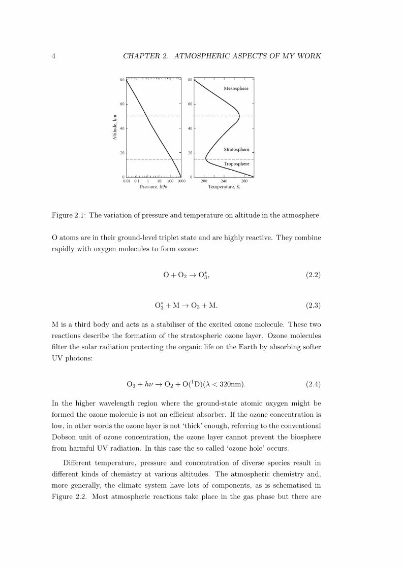
pressure and temperature in function of altitude can be seen in Figure 2.1[2].
Earth’s surface is warmed by absorbing solar radiation mainly in the infrared (IR)
range. The warm surface heats the lower region of the troposphere by convection.
Above the surface, the temperature decreases nearly linearly by increasing altitude.
The tendency changes at the altitude of about 15 km. This region is the boundary of
the stratosphere and the troposphere and is called tropopause. Above this region the
stratosphere is heated by exothermic photochemical reactions. Strong UV photons
of a wavelength smaller than 240 nm are mainly absorbed by oxygen molecules
producing atomic oxygen:
O2 + hν → 2O(3P)(λ < 240nm). (2.1)
3
4 CHAPTER 2. ATMOSPHERIC ASPECTS OF MY WORK
Figure 2.1: The variation of pressure and temperature on altitude in the atmosphere.
O atoms are in their ground-level triplet state and are highly reactive. They combine
rapidly with oxygen molecules to form ozone:
O + O2 → O∗3, (2.2)
O∗3 + M→ O3 + M. (2.3)
M is a third body and acts as a stabiliser of the excited ozone molecule. These two
reactions describe the formation of the stratospheric ozone layer. Ozone molecules
filter the solar radiation protecting the organic life on the Earth by absorbing softer
UV photons:
O3 + hν → O2 + O(1D)(λ < 320nm). (2.4)
In the higher wavelength region where the ground-state atomic oxygen might be
formed the ozone molecule is not an efficient absorber. If the ozone concentration is
low, in other words the ozone layer is not ‘thick’ enough, referring to the conventional
Dobson unit of ozone concentration, the ozone layer cannot prevent the biosphere
from harmful UV radiation. In this case the so called ‘ozone hole’ occurs.
Different temperature, pressure and concentration of diverse species result in
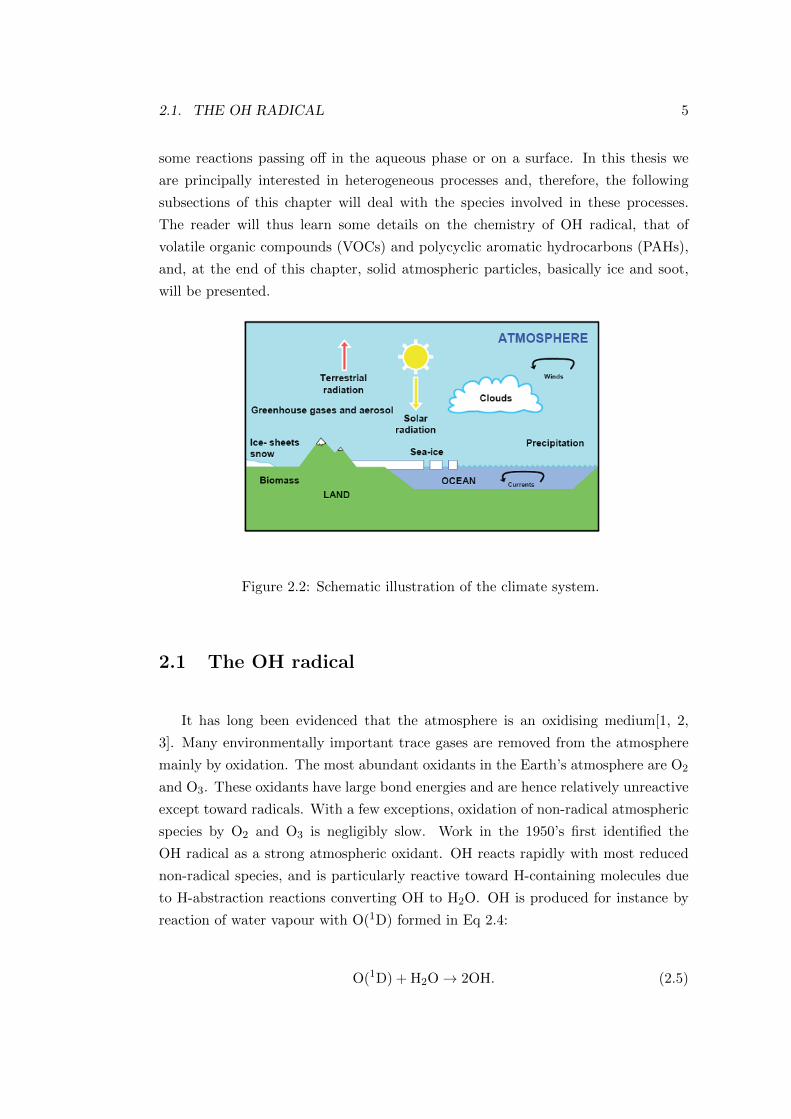
different kinds of chemistry at various altitudes. The atmospheric chemistry and,
more generally, the climate system have lots of components, as is schematised in
Figure 2.2. Most atmospheric reactions take place in the gas phase but there are
2.1. THE OH RADICAL 5
some reactions passing off in the aqueous phase or on a surface. In this thesis we
are principally interested in heterogeneous processes and, therefore, the following
subsections of this chapter will deal with the species involved in these processes.
The reader will thus learn some details on the chemistry of OH radical, that of
volatile organic compounds (VOCs) and polycyclic aromatic hydrocarbons (PAHs),
and, at the end of this chapter, solid atmospheric particles, basically ice and soot,
will be presented.
Figure 2.2: Schematic illustration of the climate system.
2.1 The OH radical
It has long been evidenced that the atmosphere is an oxidising medium[1, 2,
3]. Many environmentally important trace gases are removed from the atmosphere
mainly by oxidation. The most abundant oxidants in the Earth’s atmosphere are O2
and O3. These oxidants have large bond energies and are hence relatively unreactive
except toward radicals. With a few exceptions, oxidation of non-radical atmospheric
species by O2 and O3 is negligibly slow. Work in the 1950’s first identified the
OH radical as a strong atmospheric oxidant. OH reacts rapidly with most reduced
non-radical species, and is particularly reactive toward H-containing molecules due
to H-abstraction reactions converting OH to H2O. OH is produced for instance by
reaction of water vapour with O(1D) formed in Eq 2.4:
O(1D) + H2O→ 2OH. (2.5)
6 CHAPTER 2. ATMOSPHERIC ASPECTS OF MY WORK
Critical to the generation of OH is the tropospheric production of excited O(1D)
atoms in Eq 2.4, which is considerably slower than in the stratosphere. To complete
the mechanism one should take into account the deactivation of the excited O atom
by a neutral molecule, which leads to the loss of O(1D) slowing down Eq 2.5:
O(1D) + M→ O + M. (2.6)
The slow formation and the deactivation of the excited O atom are compensated by
the large H2O mixing ratio compared to the stratosphere. Accurate estimation of
the mean OH concentration established 1.2× 10⁶ molecules cm−3[2], and supported
its importance as an oxidant in the troposphere. The mean lifetime of a given com-
pound can be estimated in terms of the dominant reactions consuming it. CO turned
out to be the principal sink of OH in most of the troposphere and CH4 is next in
importance. These two gases therefore play a critical role in controlling OH con-
centration and more generally in driving radical chemistry in the troposphere. The
resulting lifetime of OH is of the order of one second. Due to this short atmospheric
lifetime, concentrations of OH are highly variable; they respond rapidly to changes
in sources and sinks.
Atmospheric chemists suspected for a long while that there should be another
substantial source of OH in the troposphere apart from Eq 2.5 and the stratospheric
ozone supply because they seemed to be insufficient to prevent CO, CH4 and other
greenhouse gases from accumulating to very high levels in the troposphere, with
catastrophic environmental implications.
A key factor in this prevention is the presence of trace levels of NOx (= NO
+ NO2) originating from combustion, lightning and soils. This key factor allows
the regeneration of OH consumed in the oxidation of CO and hydrocarbons, and
concurrently provides a major source of O3 in the troposphere. The main steps of
this chain mechanism can be summarised in the following reactions:
CO + OHO2→ CO2 + HO2, (2.7)
HO2 + NO→ HO + NO2, (2.8)
NO2 + hνO2→ NO + O3. (2.9)
The resulting net reaction is:
2.1. THE OH RADICAL 7
CO + 2O2 + hν → CO2 + O3. (2.10)
The net result is the production of ozone where the oxidation of CO by O2 is catalysed
by the HOx chemical family (HOx = H + HO + HO2), whereas the OH regeneration
is catalysed by NOx. The resulting O3 can generate additional OH.
In contrast, a considerably different behaviour can be observed in the stratosphere
where HOx family catalyses ozone loss procedures. The hydroxyl radical produced
in Eq 2.5 can react with ozone producing the hydroperoxy radical that reacts with
another ozone molecule:
OH + O3 → HO2 + O2, (2.11)
HO2 + O3 → OH + 2O2, (2.12)
Net : + 2O3 → 3O2. (2.13)
Recent work has shown that this HOx-catalysed mechanism represents, in fact,
the dominant sink of ozone in the lowest stratosphere[3]. The basically different
behaviour between the troposphere and the stratosphere arises from the fact that
O3 and O concentrations are much lower in the troposphere thus ozone destruction
processes are a couple of orders or magnitude slower.
In the case of CH4 the mechanism is much more complicated and is conducted
through formaldehyde, organic peroxides and peroxide radicals. If we consider an
atmosphere rich in NOx one can yield the following net reaction for the conversion
of CH4 to CO2:
CH4 + 10O2 → CO2 + 5O3 + 2OH. (2.14)
The assumption of the high NOx concentration (high-NOx regime) results in five
ozone molecules and two OHs per methane molecule. In contrast, if we examine an
atmosphere deficient in NOx the resulting net reaction can be written as
CH4 + 3OH + 2O2 → CO2 + 3H2O + HO2. (2.15)
8 CHAPTER 2. ATMOSPHERIC ASPECTS OF MY WORK
This mechanism diminishes the oxidising power of the atmosphere. These two mech-
anisms emphasize the critical role of NOx for maintaining O3 and OH concentrations
in the troposphere.
Larger hydrocarbon molecules are less important than methane because their
sources are minor compared to that of methane. They can, however, have a sig-
nificant role in rapid production of ozone in polluted regions. Their oxidation and
the oxidation of other VOCs are similar to the oxidation of methane. Complications
emerge over the diverse issues of the organic oxy (RO) and peroxy RO2 radicals and
also over the structure and fate of oxygenated organic compounds.
2.2 VOCs in the atmosphere
VOCs are emitted into the atmosphere both from anthropogenic and biogenic
sources. The most abundant VOCs emitted from anthropogenic and biogenic sources
are methane and isoprene, respectively. The former gets to the atmosphere by
fuel production and distribution, whereas the latter principally by biomass burn-
ing. Methane also has a large biogenic source. VOC may have effects on human
health, plants and animals and also on the climate of the Earth. The direct neg-
ative effects on human health from VOC are local, mainly of concern close to the
emission sources and in working environments, since it is only in these places that
high concentrations of VOC are reached. Chlorinated VOC may bioaccumulate or
may survive long enough to reach the stratosphere where they may contribute to the
ozone depletion. VOCs also influence tropospheric ozone chemistry if NOx concen-
tration is high enough. As we have seen, ozone is crucial in the stratosphere to filter
solar radiation; in the remote regions of the troposphere ozone is a non-negligible
source of OH radical that prevents green house gases (GHGs) from catastrophic ac-
cumulation. Contrary to this, ozone in surface air is a harmful secondary pollutant
and GHG. Production of O3 in polluted air follows the same chain mechanism as
described above. The chain is initiated by production of OH and propagated by
reaction of OH with VOCs. This reaction gives organic peroxy radical with the use
of an oxygen molecule:
RH + OHO2→ RO2 + H2O. (2.16)
The importance of different VOCs in atmospheric chemistry depends on their abun-
dance and their reactivity with OH. Increasing chain or unsaturated bonds increases
the reactivity.
2.2. VOCS IN THE ATMOSPHERE 9
The RO2 radical reacts rapidly with NO to produce NO2 and an organic oxy
radical:
RO2 + NO→ RO + NO2. (2.17)
The RO radical has several possible fates while NO2 goes on to photolyse and pro-
duce O3. Typically, carbonyl compounds (usually aldehydes) and HO2 radical are
produced in the reaction of RO and O2. The carbonyl compound may either photol-
yse to produce HOx or react with OH to propagate the reaction chain farther. The
net reaction is
RH + 4O2 → R′CHO + 2O3 + 2H2O. (2.18)
HO is regenerated then from HO2 by NO similarly to Eq 2.8. The chain is terminated
by the loss of the catalytic HOx radicals. This loss takes place usually by the joint
recombination of two peroxy radicals producing hydrogen peroxide:
2HO2 → H2O2 + O2. (2.19)
The fate of the different VOCs is eventually the same: they are oxidised forming
CO2 and H2O which are the strongest green house gases. Some VOCs are themselves
GHGs too. In the course of their oxidation they influence the formation of ozone
to a different extent: Photochemical ozone creation potential (POCP) quantifies
the impact of different VOCs on the ozone formation. This parameter aids envi-
ronmentalists to develop different environmental policies for different VOCs. The
determination of POCP values requires the analysis of the time evolution of the
local concentration of different species by solving coupled balance equations (usu-
ally in computer modelling studies). A useful tool for that is ‘Master chemical
mechanism’[5, 6], which contains the most important atmospheric processes and the
related rate constants. POCP is defined relative to ethane (POCP of ethane is 100
by definition) and describes how efficiently the VOC generates ozone compared with
ethane[7].
Besides the POCP value the lifetime of VOCs is also an important atmospheric
feature in connection with their atmospheric impact. This refers both to how long
they can influence the atmosphere as a GHG and the distance that VOCs are trans-
ported to. The atmospheric lifetime is defined in terms of the concentration of OH
as being the major sink for VOCs:
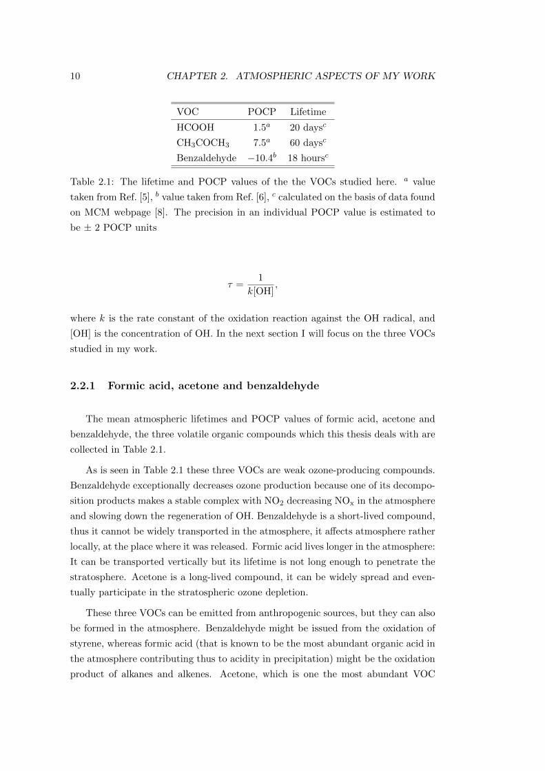
10 CHAPTER 2. ATMOSPHERIC ASPECTS OF MY WORK
VOC POCP Lifetime
HCOOH 1.5a 20 daysc
CH3COCH3 7.5a 60 daysc
Benzaldehyde −10.4b 18 hoursc
Table 2.1: The lifetime and POCP values of the the VOCs studied here. a value
taken from Ref. [5], b value taken from Ref. [6], c calculated on the basis of data found
on MCM webpage [8]. The precision in an individual POCP value is estimated to
be ± 2 POCP units
τ =1
k[OH],
where k is the rate constant of the oxidation reaction against the OH radical, and
[OH] is the concentration of OH. In the next section I will focus on the three VOCs
studied in my work.
2.2.1 Formic acid, acetone and benzaldehyde
The mean atmospheric lifetimes and POCP values of formic acid, acetone and
benzaldehyde, the three volatile organic compounds which this thesis deals with are
collected in Table 2.1.
As is seen in Table 2.1 these three VOCs are weak ozone-producing compounds.
Benzaldehyde exceptionally decreases ozone production because one of its decompo-
sition products makes a stable complex with NO2 decreasing NOx in the atmosphere
and slowing down the regeneration of OH. Benzaldehyde is a short-lived compound,
thus it cannot be widely transported in the atmosphere, it affects atmosphere rather
locally, at the place where it was released. Formic acid lives longer in the atmosphere:
It can be transported vertically but its lifetime is not long enough to penetrate the
stratosphere. Acetone is a long-lived compound, it can be widely spread and even-
tually participate in the stratospheric ozone depletion.
These three VOCs can be emitted from anthropogenic sources, but they can also
be formed in the atmosphere. Benzaldehyde might be issued from the oxidation of
styrene, whereas formic acid (that is known to be the most abundant organic acid in
the atmosphere contributing thus to acidity in precipitation) might be the oxidation
product of alkanes and alkenes. Acetone, which is one the most abundant VOC
2.3. PAH MOLECULES IN THE ATMOSPHERE 11
originating from anthropogenic sources as being a fuel additive, might also issue
from the oxidation of butane.
Their fate is similar: First they form peroxy radical in the course of their oxida-
tion by OH radical. Then formic acid gives CO2 and HO2. Benzaldehyde transforms
to, among others, benzoic acid. The depletion of acetone is very complex. It gives
methylglyoxal or decarboxylased products such as acetic acid or eventually formalde-
hyde.
2.3 PAH molecules in the atmosphere
Polycyclic aromatic hydrocarbons consist of fused aromatic rings and do not
contain hetero atoms or substituents. Conventionally, benzene is not considered to
be a PAH as having only one aromatic ring but one can use it as a model of PAH
molecules. They are principally produced as by-products of incomplete fuel burning
(either fossil fuel or biomass). As a pollutant, they are of concern because some
compounds have been identified as carcinogenic, mutagenic and teratogenic. They
are also found in the interstellar medium, in comets and in meteorites, and as a
candidate molecule, act as a basis for earliest forms of life. In graphene the PAH
motif is extended to large 2D sheets. Due to their low volatility they are found
primarily in soil, sediment and they are also a component of concern in fine particles
suspended in air (i.e. in aerosols). PAHs are among the most widespread pollutants.
Their toxicity is very structurally dependent, varying from being non toxic to being
extremely toxic.
It has been understood that the reactive fate of small and volatile PAHs is gov-
erned by gas-phase reactions with OH. However, due to their low vapour pressure
and aromaticity, heavier PAHs are mostly adsorbed on fine carbonaceous particles[9],
where they are subjected to a wide range of heterogeneous reactions which depend
upon the particle composition[10, 11]. This heterogeneous reactivity may thus be
more important than the corresponding gas phase reactions as sinks of these com-
pounds. Moreover, heterogeneous reactions of particle-bound PAHs may change the
microphysical properties of the particle by making it more hygroscopic and hence
modifying its cloud nucleation properties[12]. These heterogeneous reactions can also
influence the atmospheric residence times of the carbonaceous particles and conse-
quently their direct and indirect effects on climate[14, 4]. During the incomplete
combustion of fossil fuels, PAHs are formed concurrently with soot particles and
play a significant role in soot formation and subsequent particle growth[15]. Because
12 CHAPTER 2. ATMOSPHERIC ASPECTS OF MY WORK
PAHs have a high affinity for carbonaceous materials, adsorption of PAHs on soot
may be an important mechanism affecting both the gas-particle partitioning of PAHs
and also their reactivity.
2.4 Solid particles in the atmosphere
2.4.1 Ice particles
Water in the atmosphere is usually in a metastable supercooled state, which can
be maintained in the absence of ice forming nuclei, providing that the temperature is
higher than 231 K. In clouds containing some ice particles, water vapour can conden-
sate directly onto ice according to the Bergeron process (homogeneous nucleation).
Ice particles being large enough would be more likely to reach the surface by pre-
cipitation without evaporating. Note that homogeneous nucleation of ice particles
directly from water vapour can also occur at very low temperature, typically less
than 190 K, i.e., in the stratosphere above polar regions. This homogeneous freezing
of ice particles participate in the occurrence of Polar Stratospheric Clouds (PSCs)
that are involved in the ozone depletion mechanisms.
Clouds play a significant role in regulating the radiation balance of the Earth–
atmosphere system, and are, hence, an important component of the Earth’s climate
system. Clouds can absorb and re-radiate outgoing terrestrial radiation, and thereby
act as a greenhouse gas. At the same time they can reflect incoming solar radiation
back to space thus in other words they change the albedo (the reflective proper-
ties against the solar radiation) of the atmosphere. Which process dominates, and,
hence, the arithmetic sign of the net radiative forcing of clouds appears to be very
sensitive to the cloud microphysical and macrophysical properties[16]. Clouds can
also alter the chemical composition by uptake of different species while heteroge-
neous reactions, for example of halogen species on the surface of cloud particles, can
affect the atmospheric ozone budget[17].
In the case of heterogeneous condensation, water condensates onto so called ‘cloud
condensation nuclei’ of which number and type can affect the amount, lifetimes and
radiative properties of clouds and hence have an indirect influence on climate change;
the details of this mechanism are still not well understood but are the subject of
intensive research. Mineral dust, soot, sea salt and organic materials can act as
cloud condensation nuclei. The effects of these tiny airborne particles called aerosols
on cloud formation have been some of the most difficult aspects of weather and
climate for scientists to understand.
2.4. SOLID PARTICLES IN THE ATMOSPHERE 13
2.4.2 Atmospheric aerosols and soot particles
Atmospheric aerosols consist of solid bodies suspended in air. These solid bodies
have a radius changing from a few nanometres to hundreds of micrometres. Soot
particles are of the major representatives of fine atmospheric aerosols that are con-
sidered to have a radius less than 1 µm. Fine aerosols originate almost exclusively
from condensation of precursor gases. Besides the soot particles, organic carbon
and H2SO4 · H2O particles are other important components of fine aerosols. The
main effects of aerosols manifest basically in scattering solar radiation, which causes
the reduction of visibility. The other main impact is the perturbation of climate,
which arises by changing the albedo of the atmosphere. The impacts arising from
scattering solar radiation are usually reflected in the so called ‘radiative forcing’ ef-
fect. Radiative forcing is defined as the change in the net radiation balance at the
tropopause caused by a particular external factor. These forcing mechanisms are
caused mainly by change in the atmospheric concentration of greenhouse gases (such
as CO2, CH4 and N2O), but the change in the albedo of the climate system and
atmospheric aerosols are not negligible sources either.
The size, concentration and chemical composition of atmospheric aerosols are
quite diverse. Some aerosols are emitted directly into the atmosphere while others are
formed in the air. Although the radiative forcing effect of aerosols can be changing,
they are considered in average to have a negative effect (i.e. they decrease the
temperature). Their direct radiative forcing effect comes form (elastic and inelastic)
light scattering, which results finally in a decrease of solar radiation reaching the
Earth’s surface. The indirect effect arises from the mechanisms by which aerosols
modify the microphysical properties of clouds. These properties are related to the
efficiency of aerosols for serving as nuclei in the condensation processes of water
vapour. The nucleating properties depend on the size, the chemical composition of
aerosols, and on the surrounding.
During the last few years, numerous studies have reported the radiative forc-
ing effect of atmospheric soot particles. However, a couple of uncertainties arose
concerning the direct and indirect effects of soot due to its optical, compositional
and morphological diversity. To the best of our knowledge, the principal impact
of soot on the atmosphere comes from the formation of contrails that evolve into
artificial clouds. The formation of contrails is influenced by the altitude of flight,
the properties and quantity of the emitted particles and propulsion mode of the
aircraft etc[18, 19, 20]. The radiative effect induced by aviation is estimated to be
about 0.1 W m−2[21, 22]. In this estimation, uncertainties arise, which originate
14 CHAPTER 2. ATMOSPHERIC ASPECTS OF MY WORK
from our defective knowledge of the climatic effects of contrails. Crude estimations
provisioned an augmentation of a factor of 5 in the radiative forcing effects of the
emission of air traffic in 2050[21]. The surface of sky being covered by contrails is
estimated to be 8% of that covered by natural clouds in the main air lanes[24, 23].
As we have said, soot can serve as nuclei in the formation of ice particles. Princi-
pally, two types of nucleation can be distinguished: homogeneous and heterogeneous
nucleation. For the latter the presence of a solid particle is needed, whereas the for-
mer takes place without an initiator. Both of these two procedures depend strongly
on temperature and relative humidity. Analyses have shown that particles partici-
pating in the formation of contrails consist mainly of carbon, which suggests the key
role of soot particles in the nucleation[29, 26].
It has been evidenced that an activation of the soot surface is necessary to serve as
a condensation nucleus[29, 26]. It means that there should be some hydrophilic sites
at the soot surface, as was supported in 1987 by FTIR studies showing the presence
of carboxyl groups at the surface of soot particles resulted from the oxidation of
n-hexane by ozone[27, 28]. Earlier, an activation of the soot surface by sulphuric or
nitric acid was considered to be necessary[29, 25, 30]. More recent studies evidenced
that soot particles, issued from the combustion of decane, can adsorb water in the
absence of oxidising acids[31]. These results suggest the presence of hydrophilic sites
(structural defects, pores[32] or chemical groups) on or in the soot particles that are
able themselves to attract water molecules.
From a structural point of view, three types of pores can be distinguished in
soot: Macropores have a radius greater than 50 nm. Strong interaction between
the adsorbent and adsorbate is needed for the adsorption at these sites (similarly to
planar surfaces). Mesopores are considered to have a radius between 2 and 50 nm.
In these pores capillary condensation may occur. Micropores are smaller than 2 nm;
confinement effects are most pronounced here.
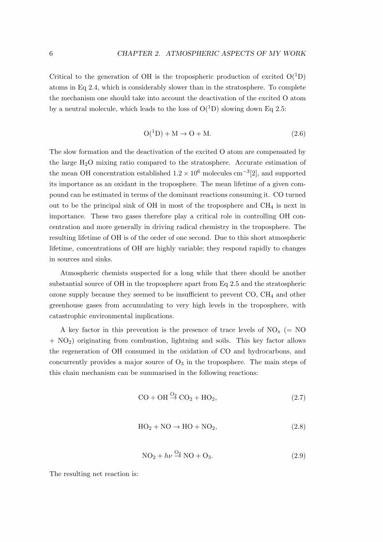
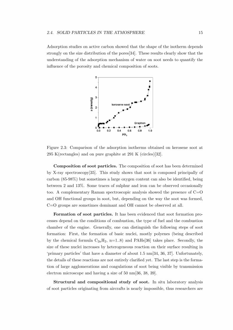
Adsorption isotherms of water on soot can support the hydrophilic character of
soot as was done by comparing the adsorption isotherm of soot originated from the
combustion of kerosene[32] and that of pure graphite[33]. The two isotherms can be
seen in Figure 2.3. This graph suggests that the absence of defects on pure graphite
results in very low affinity for water molecules. In contrast, the isotherm of the
kerosene soot indicates the filling up of the smallest micropores and the adsorption
of water molecules at the surface sites in the low pressure regime. The second
part (relative humidity being between 0.1 and 0.7) corresponds to the adsorption
of further water molecules around water molecules adsorbed previously serving as
‘secondary sites’; on the other hand, condensation in larger micropores takes place.
2.4. SOLID PARTICLES IN THE ATMOSPHERE 15
Adsorption studies on active carbon showed that the shape of the isotherm depends
strongly on the size distribution of the pores[34]. These results clearly show that the
understanding of the adsorption mechanism of water on soot needs to quantify the
influence of the porosity and chemical composition of soots.
Figure 2.3: Comparison of the adsorption isotherms obtained on kerosene soot at
295 K(rectangles) and on pure graphite at 291 K (circles)[32].
Composition of soot particles. The composition of soot has been determined
by X-ray spectroscopy[35]. This study shows that soot is composed principally of
carbon (85-98%) but sometimes a large oxygen content can also be identified, being
between 2 and 13%. Some traces of sulphur and iron can be observed occasionally
too. A complementary Raman spectroscopic analysis showed the presence of C=O
and OH functional groups in soot, but, depending on the way the soot was formed,
C=O groups are sometimes dominant and OH cannot be observed at all.
Formation of soot particles. It has been evidenced that soot formation pro-
cesses depend on the conditions of combustion, the type of fuel and the combustion
chamber of the engine. Generally, one can distinguish the following steps of soot
formation: First, the formation of basic nuclei, mostly polyenes (being described
by the chemical formula C2nH2, n=1..8) and PAHs[36] takes place. Secondly, the
size of these nuclei increases by heterogeneous reaction on their surface resulting in
‘primary particles’ that have a diameter of about 1.5 nm[34, 36, 37]. Unfortunately,
the details of these reactions are not entirely clarified yet. The last step is the forma-
tion of large agglomerations and coagulations of soot being visible by transmission
electron microscope and having a size of 50 nm[36, 38, 39].
Structural and compositional study of soot. In situ laboratory analysis
of soot particles originating from aircrafts is nearly impossible, thus researchers are
16 CHAPTER 2. ATMOSPHERIC ASPECTS OF MY WORK
restrained to study soot produced in laboratory. Usually, for laboratory purposes
kerosene is too expensive. On the other hand, instead of aircraft engine combustion
chambers or burners are used. These facts lead to a great variety of results, which
are sometimes even contradictory. To facilitate the research concerning soot, some
experimental protocols for soot generation have been used over the last few years.
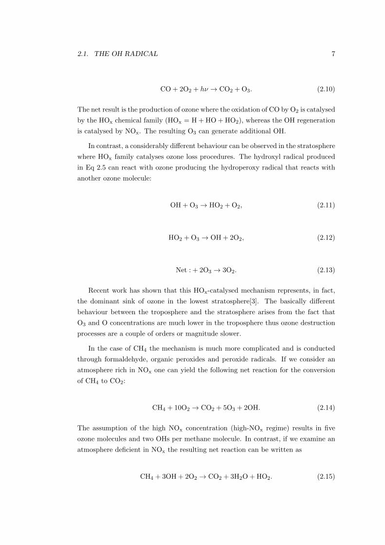
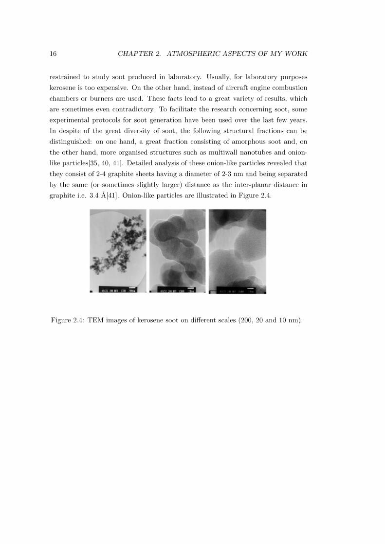
In despite of the great diversity of soot, the following structural fractions can be
distinguished: on one hand, a great fraction consisting of amorphous soot and, on
the other hand, more organised structures such as multiwall nanotubes and onion-
like particles[35, 40, 41]. Detailed analysis of these onion-like particles revealed that
they consist of 2-4 graphite sheets having a diameter of 2-3 nm and being separated
by the same (or sometimes slightly larger) distance as the inter-planar distance in
graphite i.e. 3.4 A[41]. Onion-like particles are illustrated in Figure 2.4.
Figure 2.4: TEM images of kerosene soot on different scales (200, 20 and 10 nm).
Chapter 3
Computational methods
3.1 Computer simulation methods
Statistical physics aims at describing the macroscopic properties of a system on
the basis of the microscopic characteristics of every particle constituting the system.
This objective requires, however, unimaginably great amounts of information about
the system. One would have to entirely know the position and momentum of each
particle at each moment of time. The knowledge of this amount of information is
clearly impossible. But even if one knew all information a second problem, rather
of a mathematical nature, would arise: the integration of nearly infinite microscopic
properties seems to be unachievable. Statistical physics, however, proved to be a
useful tool for the description of reality. Reasonable approximations for the average
behaviour of particles constituting the system made it applicable in numerous cases.
Computer simulation techniques are obvious tools for the application of the equa-
tions of statistical physics because no approximation has to be used to gain the av-
erage properties of the system. It is possible to determine them by observation of
the motion of the particles during the simulation. This is why computer simulations
are often called numerical experiments. Limitations come from the restricted num-
ber of particles observed in the simulation and also from the limited time available
for the simulation. Nevertheless, there are properties that can be quite accurately
calculated in a finite system during a finite simulation time.
There are two principal ways to determine the average properties of the system.
One may calculate them as a mean value integrated either in time or over the en-
semble of microstates of the entire phase space. The former needs almost infinitely
long simulation to guarantee the system passes through all microstates of the phase
17
18 CHAPTER 3. COMPUTATIONAL METHODS
space (i.e. the system fulfills the requirement of ergodicity), whereas the latter ne-
cessitates the knowledge of the probability of being in each microstate of the phase
space. The ergodic hypothesis states the equality of the time average gained by the
first approach and the ensemble average yielded by the second:
〈A〉t = limτ→∞
1
τ
∫ τ
0dtA(q(t),p(t)) =
∫dqdpA(q,p)f(q,p) = 〈A〉Γ , (3.1)
where p and q denote the momenta and the spatial coordinates of all particles
respectively; A(q,p) represents the value of quantity A at the Γ ≡q,p point (i.e.
a microstate) of the phase space, 〈A〉 is the mean (i.e. macroscopic) value of A;
f(q,p) is the probability density function over the microstates, t is the time while
τ is the duration of observation. In the above equation the left hand side gives the
principle of molecular dynamics, while the right hand side gives that of Monte Carlo
method.
Both techniques need the generation of microstates of the system being described
by the same macroscopic state functions. In molecular dynamics (MD)[42] methods
the generation of microstates is done by the numerical integration of the equations
of motion of each particle of the system for a short time step (usually in the order of
a femtosecond). The integration gives the new molecular positions of the particles.
Here, the atomic configurations generated step by step have time correlation and they
depend on the previous configurations. This feature makes the molecular dynamics
methods capable of calculating dynamical, time-dependent properties besides time-
independent ones. During the simulation, the system visits the microstates of the
phase space available as frequently as is dictated by the probability density function
(if the simulation is long enough). One can also simulate non-equilibrium processes
with this method. The drawback is that the calculation of forces and the numerical
integration are quite time consuming.
On the contrary, Monte Carlo (MC)[42] methods are considered to be stochastic
methods. Here, the generation of a new configuration is accomplished by a random
change in the current configuration of the system. Then the generated configuration
will be accepted or rejected according to the acceptance criterion. Because the
generation of the new configuration needs only the knowledge of the current one
(and not of the previous ones), the set of the configurations has no memory. It is
therefore impossible to simulate non-equilibrium processes with MC methods. Due
to the lack of explicit appearance of time in the equations of the MC method, it is
also impossible to obtain time-dependent quantities with MC methods. The great
3.1. COMPUTER SIMULATION METHODS 19
advantage of MC methods in contrast with MD is rapidity: the time needed for an
MC step is 1-2 orders of magnitude smaller than that of MD.
3.1.1 Monte Carlo method
MC methods are widely used in science where random sampling from a given
ensemble may yield the approximate solution to a problem. In physics usually one
has to sample from the phase space according to the probability density function,
which can be given as
f(q,p) =exp(−βF(q,p))∫
dqdp exp(−βF(q,p))=
1
N !h3N
exp(−βF(q,p))
Q, (3.2)
where β= 1kBT
, kB denotes the Boltzmann constant and F(q,p) is an energy-like
potential function depending on the boundary conditions of the thermodynamical
ensemble of the system. Q is the normalising factor of the density function and is
often called partition function:
Q =1
N !h3N
∫dqdp exp(−βF(q,p)). (3.3)
In the above equations the division by N ! is needed to take into account that the
permutation of N particles constituting the system does not increase the number of
microstates, whereas the factor h3N accounts for the fact that within a unit volume
of this size in the phase space the quantum states are already indistinguishable, thus
the number of microstates must be reduced by this factor.
Because only position-dependent quantities can be obtained the sampling nar-
rows only to the position-dependent part of the phase space (which is often called
configurational space), and the momentum-dependent parts can be separated and
integrated out of the density function. The mean value of A takes the following form:
〈A〉 = ((((((((((∫dp exp(−βFp(p))
∫dqA(q) exp(−βFq(q))
((((((((((∫dp exp(−βFp(p))
∫dq exp(−βFq(q))
=
∫dqA(q) exp(−βFq(q))∫
dq exp(−βFq(q)),
(3.4)
where Fp(p) is the momentum-dependent, while Fq(q) is the position-dependent
part of the potential function, fulfilling F(q,p) ≡ Fp(p)Fq(q). The denumerator
here is often called configurational integral. Instead of the integration one may
write summation in Eq 3.4 because in practice, one would study only a finite set of
configurations:
20 CHAPTER 3. COMPUTATIONAL METHODS
〈A〉 =
∑i∈S A(qi) exp(−βFq(qi))∑
i∈S exp(−βFq(qi)), (3.5)
where i runs over all atomic configurations (microstates) qi in set S. At this point,
further refinement of the method is necessary, otherwise the contributions of the
entirely random configurations to the mean value of A would likely be very small
due to the high value of Fq(qi). This is related to the likely ‘unphysical’ struc-
tures generated randomly, which results in a small statistical factor (that decreases
exponentially with Fq), so the convergence of the mean value would be very very
slow. The trick one has to use here was first described by Metropolis and co-workers
and is that configurations with relatively low Fq value are more likely to be chosen,
which results in distortion of the randomness of the sampling. The distortion can
be corrected thus:
〈A〉 =
∑i∈S A(qi)
exp(−βFq(qi))wi∑
i∈Sexp(−βFq(qi))
wi
, (3.6)
where wi is the sampling weight factor of the ith configuration. If this factor equals
just exp(−βFq(qi)) the weighted expectation value of the quantity A becomes simply
the arithmetic mean of the A(qi) values.
One thus gains on one hand, the rapid convergence of the expectation value and,
on the other hand, the simplicity of the expression at the expense of the biased
Metropolis algorithm. As an example, we will demonstrate how this algorithm is
applied in the simplest case, i.e., in the case of the canonical (N,V, T ) ensemble.
Since the energy-like potential function related to the canonical ensemble is the
total energy itself, its position-dependent part is simply the potential energy (i.e.,
Fq ≡ U), and thus the sampling factor becomes
wi(qi) = exp(−βU(qi)). (3.7)
The procession of the algorithm starts with making a random change in the initial
configuration. In the second step, the calculation of the potential energy correspond-
ing to the new atomic configuration is performed. Thirdly, if the potential energy
decreases the new configuration is always accepted. Otherwise it is accepted only
by a probability of exp(−β∆U(q)), and is rejected by (1 − exp(−β∆U(q))), where
∆U(q) is the difference in potential energy between the current and previous state of
the system (and is positive in this case). In practice, we generate a random number
3.1. COMPUTER SIMULATION METHODS 21
ξ between 0 and 1. If ξ is greater than exp(−β∆U(q)) the generated configuration
is rejected, otherwise it is accepted. The acceptation probability can be represented
thus as
Pacceptance = min(1, exp(−β∆U(q))). (3.8)
One can demonstrate that, if the algorithm proceeds in this way, the sampling is
indeed done according to the probability density function of the microstates[43]. In
the next subsection we will demonstrate how the Metropolis algorithm is applied on
the grand canonical ensemble.
3.1.1.1 Grand canonical Monte Carlo method
This method was developed independently by Norman and Filinov[44] and also
by Adams[45, 46].
Instead of the number of particles, the chemical potential is kept constant here
together with the temperature and volume. The condition of being in equilibrium
of a system on this ensemble is the minimality of the grand potential defined as
Ω = A−Nµ = −pV, (3.9)
where A is the Helmholtz free energy, N is the number of particles, µ is the chemical
potential, p is the pressure, and V is the volume of the system. The grand canonical
partition function is given as
Ξ =∞∑N=1
1
N !h3N
∫dqdp exp(β(Nµ− E(q,p))), (3.10)
whereas the expectation value of an arbitrary macroscopic quantity is
〈A〉 =
∑∞N=1
1N !h3N
∫dqdpA(q,p) exp(β(Nµ− E(q,p)))
Ξ, (3.11)
where E is the energy of the system. On the grand canonical ensemble, contrary to
the canonical ensemble, one has to sample from phase spaces of different numbers
of particles having the same chemical potential. After having integrated out the
momentum-dependent part of the density function and that of the partition function,
the resulting coefficient(
2πmβ
)3N/2(m denoting the mass of a single particle) does
not cancel out due to the changing number of particles. Therefore, one gets
22 CHAPTER 3. COMPUTATIONAL METHODS
〈A〉 =
∑∞N=1
1N !
(2πmβh2
)3N/2 ∫dqA(q) exp(β(Nµ− U(q)))
∑∞N=1
1N !
(2πmβh2
)3N/2 ∫dq exp(β(Nµ− U(q)))
. (3.12)
Conventionally, the following notation can be introduced:
Λ =
√βh2
2πm, (3.13)
this quantity is often referred to as the thermal de Broglie wavelength. It is conve-
nient to use scaled coordinates instead of spatial ones:
s = qV 1/3, (3.14)
where s and q denote only one coordinate of a particle. Using these notations Eq 3.12
takes the following conventional form:
〈A〉 =
∑∞N=1
∫dsA(s) V N
N !Λ3N exp(β(Nµ− U(s)))∑∞N=1
∫ds V N
N !Λ3N exp(β(Nµ− U(s))). (3.15)
The sampling weight factor is thus in this case:
wi(s, N) =V N
N !Λ3Nexp(β(Nµ− U(s))) =
= exp
[N ln
(V
Λ3
)− ln(N !)− β(U(s)−Nµ)
]. (3.16)
In the grand canonical MC technique there are three different types of move: i)
a particle is displaced; ii) a particle is destroyed (no record of its position is kept);
iii) a particle is created at a random position in the system. Thus the acceptance
ratio is:
Pacceptance = min
1, exp
[∆
(N ln
(V
Λ3
)− ln(N !)− β(U(s)−Nµ)
)]. (3.17)
which reduces to the normal Metropolis method in the case of particle displacement
(∆N = 0):
3.1. COMPUTER SIMULATION METHODS 23
Pacceptance = min(1, exp(−β∆U(s))). (3.18)
The acceptance of the addition or removal of more than one particle proved to be
very improbable in dense systems[44], thus in one step, the creation or destruction
of only one particle is attempted. The acceptance criterion in these cases becomes
Pacceptance = min
1, exp
[ln
(V
Λ3
)− ln(N + 1)− β(∆U(s)− µ)
], (3.19)
in the case of creation (i.e. ∆N = 1), and
Pacceptance = min
1, exp
[− ln
(V
Λ3
)+ ln(N)− β(∆U(s) + µ)
]. (3.20)
in the case of destruction (i.e. ∆N = −1).
The condition of microscopic reversibility can be satisfied by making the proba-
bility of an attempted creation equal to the probability of an attempted destruction.
Norman and Filinov suggested setting the probability of attempting the three moves
equal, because fastest convergence can be achieved in this way.
The great advantage of the GCMC method is that equilibria in highly inhomo-
geneous systems, such as adsorption processes or membranes are easy to simulate.
It should be noted that the Monte Carlo method is dominant as opposed to the
molecular dynamics on the grand canonical ensemble because the destruction and
creation of particles sets serious technical problems in dynamical simulations.
With increasing density the probability of successful creation or destruction steps
becomes small. Creation attempts fail because of the high risk of overlap. Destruc-
tion in the vicinity of a surface may be also infrequent and this somewhat offsets the
advantage of GCMC in the simulation of adsorption. To address these problems,
Mezei[47, 48] extended the basic method to search for cavities in the system which
are of an appropriate size to support the creation. Once these cavities are located,
creation attempts are only made inside the cavities. This method is referred to as
the cavity-biased GCMC method.
It should be noted that a reformalisation of the GCMC method suggested by
Adams for the chemical potential can be used, which splits it into the ideal gas and
excess part:
24 CHAPTER 3. COMPUTATIONAL METHODS
µ = µex + µid = µex + kT
[ln 〈N〉µ,V,T + ln
(Λ3
V
)]= kTB + kT ln
(Λ3
V
), (3.21)
where B accounts for the terms that are not known usually at the beginning of the
simulation such as the excess chemical potential and the average number of a given
molecule type:
B ≡ µex
kT+ ln 〈N〉µ,V,T , (3.22)
and, on the other hand, as a consequence of Eq 3.21:
B =µ
kT− ln
(Λ3
V
). (3.23)
Adams performed grand canonical Monte Carlo simulations at constant B, T
and V where B is defined in the above equations. It is obvious that this technique
is completely equivalent to the method at constant µ, T and V .
3.1.2 Molecular dynamics
In molecular dynamics simulations, the next configuration of the system is gener-
ated by solving the equations of motion of each particle in the system. First, one has
to define the Hamiltonian of the system that exists for all mechanical systems. The
Hamiltonian H is the total energy of the system, thus, it is the sum of the kinetic
energy K and potential energy U ; in classical mechanics:
H(q,p) ≡ K(p) + U(q). (3.24)
The equations of motion in the Hamiltonian formalism are
qi =∂H(q,p)
∂pi=
pi
mi, (3.25)
pi = −∂H(q,p)
∂qi= −∂U(q)
∂qi≡ Fi, (3.26)
where qi, pi and mi are the location, the momentum and the mass of the ith particle
respectively. Eq 3.25 and Eq 3.26 describe a system of 6N first order differential
3.1. COMPUTER SIMULATION METHODS 25
equations. The analytical solution of this system of equations is impossible, therefore
numerical methods should be applied.
Many methods were introduced to solve these equations, in all of which the
simulation proceeds by alternately calculating forces and solving the equations of
motion based on the accelerations obtained from the new forces. For example, in the
Verlet-Stormer algorithm, Eq 3.26 is solved directly[49]. First, writing the Taylor
expansion of the coordinate vector at t0 + ∆t and t0 −∆t around time t0
qi(t0 + ∆t) =∞∑n=0
(∆t)n1
n!
∂nqi
∂tn(t0), (3.27)
qi(t0 −∆t) =∞∑n=0
(−1)n(∆t)n1
n!
∂nqi
∂tn(t0), (3.28)
and, adding them up, only the even-order terms remain:
qi(t0 + ∆t) = 2qi(t0)− qi(t0 −∆t) + (∆t)2qi(t0) +O((∆t)4
). (3.29)
According to this algorithm, to calculate the position of atom i at the next time
step, one has to use the current and previous position and the current acceleration
coming from the force applied on particle i. If one does so, the algorithm error
occurs only in fourth order. However, this algorithm has a great drawback, namely
that the error of the velocity in the next moment is of second order. Therefore,
predictor-corrector methods are usually applied to overcome this problem. For the
integration it is fundamental to choose an appropriate time step length ∆t, which
has to be in the same order of magnitude as the time scale of the studied particle
motions; in molecular systems the value of ∆t is typically around 0.5− 2 fs.
3.1.3 Potential models used
The importance of the potential model in classical simulations is emphasised
because it determines the behaviour of not only each single particle but that of the
whole system as well, and it eventually also defines the entire structure of the system.
The potential has to be differentiable, since forces are calculated as its derivatives
and, on the other hand, differentiation should be quick to ensure the efficiency of
the simulation. In classical simulations classical potentials are used, which may be
adjusted to different (usually experimental) properties of the macroscopic system
to be simulated. These potentials are thus able to reproduce some properties well
26 CHAPTER 3. COMPUTATIONAL METHODS
and some others less well. Classical potentials may not reproduce properties well
that they are not designed for, the potential used therefore always has to be chosen
circumspectly.
There are two main groups of potentials: The first, widely used group is that of
non-reactive potentials that describe bonded and non-bonded interactions, but can-
not change the atomic environment of the particles. The second group incorporates
the reactive potentials, which can reproduce bond breaking and forming together
with bonded and non-bonded interactions.
3.1.3.1 Non-reactive potentials
The potential energy in the whole system can be given as[42]
U(q) =N∑i=1
u1(qi) +N∑i=1
N∑j>i
u2(qi,qj) +N∑i=1
N∑j>i
N∑k>j>i
∆u3(qi,qj ,qk) + ...+
+∆uN (q1,q2, ...,qN ). (3.30)
The first summation of the equation describes the effect of an external potential,
while the second term sums the pair interactions of all possible particle pairs. The
third term (∆u3) contains the additional energy of particle triplets compared to
isolated pairs. Obviously, the list has to be continued until the final term, which
includes the interaction of all the N particles not included in the previous sums.
Although this expression is exact, it cannot be used because the form of the terms
in the above equation is unknown.
In practice, the potential is approximated by the sum of, at most, pairwise ad-
ditive terms:
U(q) ≈N∑i=1
u1(qi) +N∑i=1
N∑j>i
ueff2 (qi,qj). (3.31)
The term ueff2 (qi,qj) does not equal u2(qi,qj) in Eq 3.30, and it is often called
effective pair potential, and accounts also for the contribution of multi-particle terms
to the potential energy in an average way. If there is no external field, the first term
can be neglected, while in the case of an isotropic system, the effective pair potential
depends only upon the distance between two particles rij :
3.1. COMPUTER SIMULATION METHODS 27
U(q) ≈N∑i=1
N∑j>i
ueff2 (rij). (3.32)
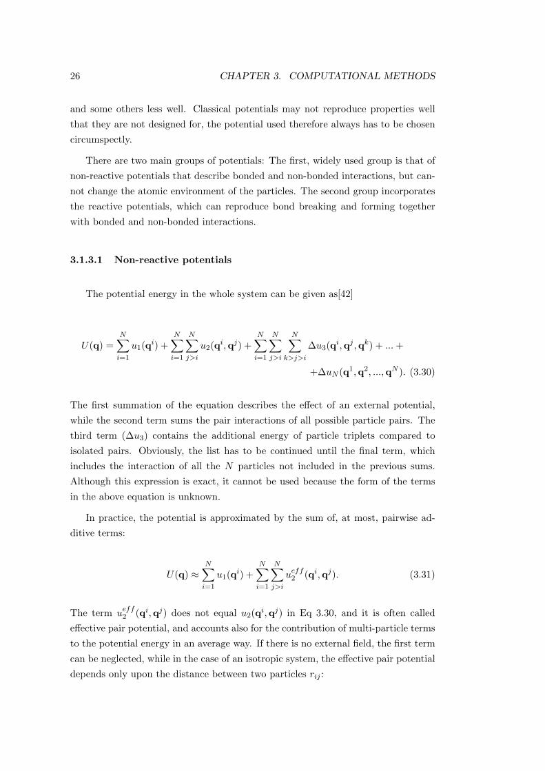
There are numerous pair potentials in the literature. The simplest one is the
hard sphere potential, which creates no interaction between two particles if they
are farther from each other than a distance r, where an infinite repulsion arises
between them. Other common pair potentials exist with a simple attractive part,
such as a constant or a linearly changing attraction in a distance range (e.g. square-
well or triangle-well potential). Although these potentials are very simple, they
are capable of reproducing some basic properties of real systems, such as solid-fluid
phase transition[42]. Clearly, to study realistic systems a more sophisticated and
continuously changing pair potential function is needed. The Morse potential or
more often the Lennard-Jones potential is a suitable choice for this purpose:
ULJ(r) = 4ε
[(σ
r
)12
−(σ
r
)6], (3.33)
where σ and ε are parameters, representing the ‘size’ of the particle and the ‘strength’
of the attraction respectively. These simple pair potentials are illustrated in Fig-
ure 3.1.
Figure 3.1: Some simple pair potentials: hard sphere potential (a), square-well po-
tential (b), triangle potential (c) and Lennard-Jones potential (d).
Usually, interaction parameters are defined between the same type of interaction
sites, thus to calculate those between different sites, the mixing of parameters is
needed. The most widely used mixing rule is the Lorentz-Berthelot rule[42]:
εAB =√εAεB and σAB =
σA + σB2
. (3.34)
In the case of charged particles the electrostatic part of the interaction also has
to be calculated. Although quite sophisticated methods have been developed based
28 CHAPTER 3. COMPUTATIONAL METHODS
on the distribution of electric multipole moments on different sites of the interacting
molecules these last years to calculate the electrostatic interactions between two
charged species[50], the simple Coulomb law involving only charge distributions on
the interaction sites is still widely used due to its simplicity. The Coulomb equation
reads:
UC(r) =1
4πε0
qAqBr
, (3.35)
where ε0 is the vacuum permittivity, qA and qB are the charges of interaction sites
A and B.
Note finally, that a series of potential models has also been developed to take into
account polarisation effects in numerical simulations. However, the introduction of
such models in numerical codes is a non trivial task. Furthermore, the correspond-
ing results are not necessarily better than those obtained when using simple pair
potentials because an accurate parametrisation of the polarisable potentials is quite
difficult to achieve. Of course, these polarisation effects may be of great importance
when simulating systems containing a net charge, such as ions.
3.1.3.2 Reactive potentials
Reactive potentials are efficient in the classical simulation of chemical reactions
by empirical modeling of changes in covalent bonding. The principle of reactive po-
tentials is that they switch on chemical forces at a certain distance where non-bonded
interactions are repulsive due to the overlap of particles. One of the most widely
used reactive potentials is e.g. empirical valence bond (EVB) potential developed
by Warshel’s group[51]. This potential was successfully used to model proton trans-
fer reactions in aqueous acids. Another example of reactive potentials is RWFF[52]
(reactive force field for water) was developed to reproduce water neutron scattering
data accurately. A third one, ReaxFF[53] was fitted to ab initio calculations and
empirical bond energies. Calculations with these force fields have been proved to
be much faster than ab initio or even semi-empirical calculations. Their accuracy is
similar to or sometimes even better than that of semi-empirical methods.
The concept of the reactive bond order (REBO) force field of Brenner[54] is simi-
lar: it takes into consideration the local coordination of atoms and the bond order of
chemical bonds in the calculation of the total energy of the system. The original goal
was to model the chemical vapour deposition of diamond films, because the mech-
anism of growth of diamond films from the vapour of hydrocarbons was not clear.
3.1. COMPUTER SIMULATION METHODS 29
Brenner developed an empirical potential energy function (based on empirical bond
energies) that captures the key features of chemical bonding in hydrocarbons, and
satisfies the following considerations. The potential i) reproduces the intermolecular
energetics and bonding in diamond, graphite and various hydrocarbons, ii) yields
realistic properties for general structures, iii) allows for bond breaking and forming,
and iv) is not computationally intensive.
The base of the method is an Abell-Tersoff potential energy expression that
was originally designed by Abell to explain universal tendencies in binding-energy
curves, with the sum of neighbour pair interactions moderated by the local atomic
environment[55]. Tersoff introduced an analytic potential energy function[56] that
realistically describes bonding in silicon for a couple of solid states. Thus the binding
energy in the Abell-Tersoff formalism is written as a sum over atomic sites i:
Eb =1
2
∑i
Ei, (3.36)
where each contribution Ei is written as
Ei =∑j 6=i
(VR(rij)−BijVA(rij)) . (3.37)
In this equation j goes over the neighbours of atom i. VR and VA are pair-additive
repulsive and attractive interactions, respectively, and Bij represents a many-body
coupling between the bond i− j and local environment of atom i. If VR and VA are
Morse-type functions, Bij can be considered a normalised bond order[56, 55] Abell
suggested, to a first approximation, that Bij can be given in function of the local
coordination Z:
Bij ∝ Z−δ, (3.38)
where δ depends on the particular system. Tersoff adjusted the pair terms and an
analytic function for Bij , and obtained quite good accuracy and transferability for
silicon, germanium and carbon. In spite of these issues, this potential has a number
of deficiencies, e.g., it is unable to properly describe conjugation and radicals.
To correct the deficiencies of the Abell-Tersoff potential Brenner suggested rewrit-
ing the above equations while maintaining the fit to diamond and graphite:
Eb =∑i
∑j>i
(VR(rij)− BijVA(rij)
), (3.39)
30 CHAPTER 3. COMPUTATIONAL METHODS
where the repulsive and attractive terms have a Morse-like form and are multiplied
by a function, which restricts the potential to nearest neighbours by switching off
the chemical forces beyond a certain distance. The empirical bond-order function is
given by the average of terms associated with each atom in a bond plus a second
term taking into account non-local effects:
Bij = (Bij +Bji)/2 + Fij(N(t)i , N
(t)j , N
(conj)ij ), (3.40)
where N(t)i and N
(t)j are the total number of neighbours (H + C) bonded to atom i
and j, respectively, while N(conj)ij depends on whether the bond i − j (between two
carbons) is part of a conjugated system, and can be even a fraction. Fij is a three-
dimensional cubic spline function to make the potential change continuously. The
Bij bond-order term depends on the number of H and C neighbours and also contains
an angle dependent part: a variety of chemical effects that affect the strength of the
covalent bonding interaction are all accounted for in this term.
For the fitting procedure, Brenner used solid state parameters of different carbon
allotrops, hydrocarbon bond energies, and heats of formation of hydrocarbons.
Despite the efficiency of the REBO potential it turned out however that it is
not appropriate, in its original form, for studying every hydrocarbon system. Since
the potential is exclusively short-ranged, the absence of dispersion and non-bonded
repulsion terms makes the potential poorly suited for any system with significant
intermolecular interactions. This is the case for many important hydrocarbon sys-
tems, including liquids and thin films. Even covalent materials such as diamond
can benefit from a treatment including non-bonded interactions. The bulk phase is
dominated by covalent interactions, but longer-range forces become quite important
when studying interfacial systems. In addition, the REBO potential also lacks a
torsional potential for hindered rotation about single bonds.
To overcome these shortcomings, Stuart modified the Brenner potential by in-
troducing non-bonded and torsional interactions through an adaptive treatment[57].
This new potential is referred to as the adaptive intermolecular REBO potential
(AIREBO). In various cases, intermolecular interactions such as dispersion and short-
range repulsion effects give rise to many of the properties of liquids, polymers and
thin-film hydrocarbon materials. In the AIREBO force field the intermolecular in-
teractions are modeled with a Lennard-Jones 12-6 potential (see Eq 3.33).
Because of the steep repulsive wall of the Lennard-Jones potential, it should be
switched off very subtly at a certain distance depending on the chemical character-
istics of the system in order to preserve the reactive nature of the potential. Three
3.1. COMPUTER SIMULATION METHODS 31
criteria were chosen to determine whether, and at what distance, to switch off the LJ
interaction. This decision is made adaptively, depending on: i) the distance separat-
ing the pair of atoms considered, ii) the strength of any bonding interaction between
them, and iii) the network of bonds connecting them. The three criteria mentioned
are represented in the following equation:
ELJij = SrijSbijCijU
LJij + (1− Srij)CijULJij (3.41)
where the factor Srij represents the distance criterion, Sbij accounts for bond order,
Cij reflects the connectivity switch, whereas ULJij is the Lennard-Jones potential
defined in Eq 3.33. Sr and Sb are cubic spline functions while C is a cosine based
switch function.
Unlike classical non-reactive potential, the reactive AIREBO potential allows the
non-bonded interaction to be turned smoothly on or off as bonding configurations
change. Usually, interactions between first (1-2), second (1-3) and third (1-4) neigh-
bours are modeled very well, thus LJ interactions are not needed. In the AIREBO
potential, however, they can be switched on smoothly through Cij if the connection
is via a series of partially dissociated bonds.
The other new component of the AIREBO potential is a term depending on
dihedral angles. The original REBO potential lacked any torsional interactions about
single bonds, representing its original focus on network solids, such as diamond and
small molecular fragments relevant to the chemical vapour deposition of diamond.
Without barrier of the rotation about single bonds the original REBO potential is
unable to properly simulate saturated hydrocarbons larger than methane.
In a reactive potential, torsional energies and barriers must change as the molecule
undergoes chemical reactions. Therefore, the symmetry of the torsional potential has
to arise naturally from the local coordination environment. This is accomplished in
AIREBO potential through the use of a torsional potential with a single minimum.
This results, for example, in a threefold symmetry of the overall torsional potential
when the torsional interactions are summed over the nine dihedral angles in a bond
between identically substituted sp3 carbons.
With the adaptive treatment of dispersion, intermolecular repulsion, and tor-
sional interactions the total energy of the system can be written in the following
form:
EAIREBO = EREBO + ELJ + Etors. (3.42)
32 CHAPTER 3. COMPUTATIONAL METHODS
This methodology presented above is an efficient tool for treating both chemical
reactivity and intermolecular interactions within the same system using a simple,
empirical potential.
3.1.4 Technical details of simulations
In this section the technical problems concerning computer simulations will be
overviewed to characterise them from a more practical point of view.
As a first step, we have to generate a configuration as the initial state of the
simulation, i.e., N particles have to be placed in the simulation cell. Usually, that
means random placement, but it can also be a crystalline structure, or – in order to
avoid errors attributed to numerical instabilities due to large initial repulsions – an
existing equilibrium structure (at least for the solvent molecules) can be used. In
the case of MD simulations, the initial velocities are set randomly according to the
Maxwell-Boltzmann distribution.
In the first part of the simulation, different properties change rapidly, and the
energy decreases. This transient part is called the equilibration period. After per-
forming a simulation for a sufficient length of time, different state functions, such as
the energy, start to fluctuate around a given value indicating that the system has
reached the equilibrium. The following part of the simulation is called the produc-
tion part, where the collection of configurations and calculation of properties are
carried out.
Unfortunately, the capacity of computers does not allow us to use an arbitrary
number of particles. Even nowadays with more powerful computers, although several
millions of atoms can be simulated, it is still a problem that too many particles appear
at the boundary of the simulation box, strongly influencing the simulation results
with boundary effects because they experience a quite different environment from
particles in the bulk phase. To highlight this problem, let us imagine 20000 atoms
being in a cubic simulation cell: Even in this case nearly 20% of the atoms are at
the faces of the box. To overcome this problem, periodic boundary conditions are
used. This means that the simulation cell is replicated and shifted by its edge length
in each direction of space, thus, it is surrounded by its own images producing an
infinite lattice.
Although this technique introduces an artificial periodicity to the system, it
eliminates boundary errors. For this purpose, the shape of the simulation box has
to be capable of filling the space without overlaps or gaps. The most standard
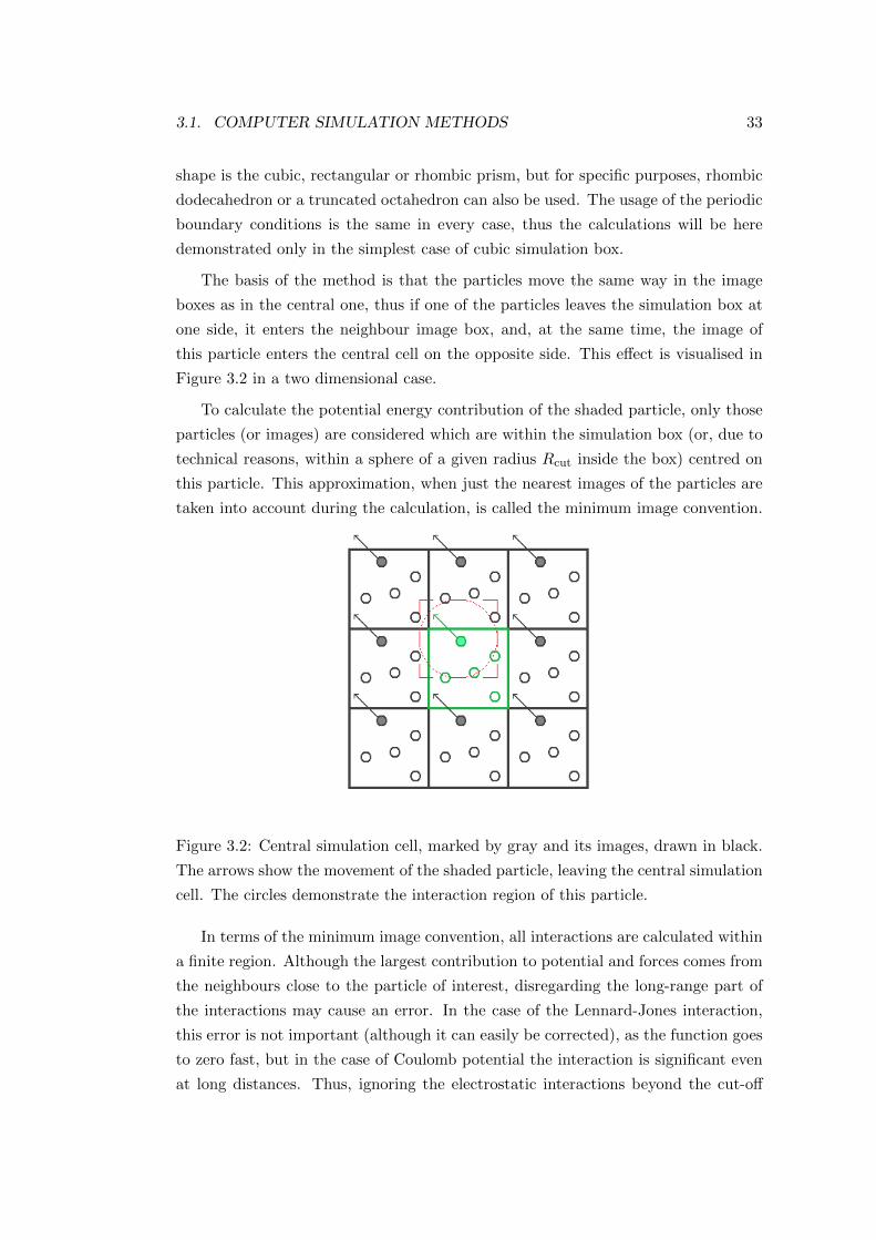
3.1. COMPUTER SIMULATION METHODS 33
shape is the cubic, rectangular or rhombic prism, but for specific purposes, rhombic
dodecahedron or a truncated octahedron can also be used. The usage of the periodic
boundary conditions is the same in every case, thus the calculations will be here
demonstrated only in the simplest case of cubic simulation box.
The basis of the method is that the particles move the same way in the image
boxes as in the central one, thus if one of the particles leaves the simulation box at
one side, it enters the neighbour image box, and, at the same time, the image of
this particle enters the central cell on the opposite side. This effect is visualised in
Figure 3.2 in a two dimensional case.
To calculate the potential energy contribution of the shaded particle, only those
particles (or images) are considered which are within the simulation box (or, due to
technical reasons, within a sphere of a given radius Rcut inside the box) centred on
this particle. This approximation, when just the nearest images of the particles are
taken into account during the calculation, is called the minimum image convention.
Figure 3.2: Central simulation cell, marked by gray and its images, drawn in black.
The arrows show the movement of the shaded particle, leaving the central simulation
cell. The circles demonstrate the interaction region of this particle.
In terms of the minimum image convention, all interactions are calculated within
a finite region. Although the largest contribution to potential and forces comes from
the neighbours close to the particle of interest, disregarding the long-range part of
the interactions may cause an error. In the case of the Lennard-Jones interaction,
this error is not important (although it can easily be corrected), as the function goes
to zero fast, but in the case of Coulomb potential the interaction is significant even
at long distances. Thus, ignoring the electrostatic interactions beyond the cut-off
34 CHAPTER 3. COMPUTATIONAL METHODS
value causes a substantial error. In order to avoid this, several correction meth-
ods were developed, from which the reaction field correction[58, 59] and the Ewald
summations[60, 61] are the most commonly used. In the reaction field correction, it
is assumed that any given molecule is surrounded by a spherical shell of finite radius
(Rcut), within which the electrostatic interactions are calculated explicitly. Outside
the spherical shell the system is treated as a dielectric continuum. The Ewald sum-
mation is a special case of the Poisson summation formula, replacing the summation
of interaction energies in real space with an equivalent summation in Fourier space.
The advantage of this approach is the rapid convergence of the Fourier-space sum-
mation compared to its real-space equivalent when the real-space interactions are
long-range.
3.2 Electronic structure calculations
If we are interested in the electronic structure of a system, or we want just
to perform a more sophisticated calculation that does not disregard the electronic
structure of the system, the tools of quantum mechanics should be used. In quantum
mechanics all systems consisting of elementary particles can be described by the
Schrodinger equation. This equation takes the following form in the case of chemical
systems, i.e., that consists only of electrons and nuclei:
H(r,R)ψ(r,R) = E(r,R)ψ(r,R), (3.43)
where r is the coordinates of all electrons, while R denotes those of all nuclei. The
above equation is an eigenvalue equation: only those states of a system are possible
that are the eigenstates (or eigenfunctions) ψ(r,R) of the Hamilton operator H. The
eigenvalue E(r,R) is just the total energy of the system corresponding to the given
eigenstate. The Hamiltonian accounts for the description of the system: it contains
the kinetic energy operator of the particles as well as all operators related to the
interactions that the particles participate in.
Normally, all motions in the system are coupled thus the motion of electrons can-
not be separated from that of nuclei. In some cases, however, it is reasonable to do
this separation by supposing that electronic motions do not affect nuclear motions.
In this case the Hamiltonian takes the form of the sum of a purely electronic and
nuclear part, while the wavefunction becomes the product of an electronic and nu-
clear wavefunction. This separation enables us to handle the electronic and nuclear
problem separately. The electronic structure can be evaluated at any given nuclear
3.2. ELECTRONIC STRUCTURE CALCULATIONS 35
configurations. This approximation is the so-called Born-Oppenheimer approxima-
tion.
To solve the electronic Schrodinger equation, one has to look for the electronic
wavefunction in an assumed form. In the simplest case, the correlation between the
electrons is neglected, each electron is treated separately. This can be reflected in
the Hartree product:
ψHartree =N∏i=1
ϕi(i), (3.44)
where i goes over all electrons N , ϕi(i) denotes the ith one-electron orbital being
occupied by the ith electron. For practical reasons, the system of N one-electron
orbitals is often chosen to be orthonormalised. To fulfil the Pauli principle, the
wavefunction has to be antisymmetric regarding the permutation of electrons. To
accomplish this requirement, instead of the product, the determinant of the one-
electron orbitals should be used:
ψSlater =1√N !
∣∣∣∣∣∣∣∣∣∣∣
ϕ1(1) ϕ2(1) . . . ϕN (1)
ϕ1(2) ϕ2(2) . . . ϕN (2)...
.... . .
...
ϕ1(N) ϕ2(N) . . . ϕN (N)
∣∣∣∣∣∣∣∣∣∣∣, (3.45)
where ϕi(j) describes the ith orbital being occupied by the jth electron and 1/√N ! is
a normalising factor. This determinant is often referred to as the Slater determinant.
It can be shown that a system of equations analogous to the Schrodinger equation
can be derived for all one-electron orbitals:
f(1, 2, . . . , N)ϕi = εiϕi, where i = 1, . . . , N. (3.46)
This equation is the canonical Hartree-Fock (HF) equation of the ith canonical or-
bital ϕi generated by the linear combination of the one-electron functions, εi is the
orbital energy, and f(1, 2, . . . , N) is the Fock operator that depends on the coordi-
nates of all electrons. This is why the system of canonical Hartree-Fock equations
can be solved only in an iterative, self-consistent manner.
Usually, we look for the eigenfunctions of the above system of equations as the
linear combinations of some beforehand chosen basis functions:
ϕi =Nb∑a=1
ca(i)χa, (3.47)
36 CHAPTER 3. COMPUTATIONAL METHODS
where a goes over the set of basis functions χa containing Nb functions, and ca(i) is
the coefficient of χa in the series of the ith orbital. With the use of this basis set, the
Hartree-Fock equations can be converted to a matrix equation, thus transforming
the problem to (iterative) matrix diagonalisation:
FCi = εiSCi, (3.48)
where Ci is the vector of all coefficients ca(i), one element of the Fock matrix F can
be written as Fab =∫
dx1χ∗a(x1)fχb(x1) (χ∗a being the complex conjugated of the
function χa and x1 being the coordinates of one electron), whereas one element of the
overlap matrix S can be written as Sab =∫
dx1χ∗a(x1)χb(x1). The above equation is
called the Hartree-Fock-Roothan equation.
Although the Hartree-Fock method is quite expressive because it supports our ap-
proach related to atomic orbitals, it cannot produce reliable and quantitative results
on many systems. One can refine this method by taking into account the electron
correlation effects but this entails the growth of the time need of these more sophis-
ticated methods (e.g. MP, CI, CC methods). On the other hand, there are large
systems for which even the Hartree-Fock method is not feasible due to the huge costs
of the calculation. There exist less sophisticated methods for these systems where the
computationally expensive terms are neglected or reasonably approximated, e.g., by
empirical formulas and parameters adjusted to experimental measurements. These
methods are called semi-empirical methods, in contrast to the purely theoretical ab
initio methods.
3.2.1 The AM1 semi-empirical method
The development of semi-empirical methods started in the 1960’s with the goal of
making molecular orbital calculations possible for large, primarily organic systems.
These methods use three main approximations as compared to the Hartree-Fock
method, namely they i) treat only the valence electrons explicitly (‘frozen core ap-
proximation’), this means one s and three p orbitals for heavy atoms, ii) use minimal
basis set, and iii) neglect the main fraction of expensive two-electron integrals and
replace the rest with empirical parameters.
The most frequently used semi-empirical methods (AM1[62], MNDO[63], PM3[64])
are all based on the Neglect of Diatomic Differential Overlap (NDDO) integral ap-
proximation. This approach belongs to the class of Zero Differential Overlap meth-
ods, in which all two-electron integrals involving two-center charge distributions are
3.2. ELECTRONIC STRUCTURE CALCULATIONS 37
neglected. The three above mentioned, most popular methods are parametrised in
such a way that the calculated energies are expressed as heats of formation instead
of total energies.
The methods based on the NDDO approximation use Slater type orbitals (STOs)
to construct the basis set:
χ(r,Θ,Φ) = Nrn−1e−ζrY ml (Θ,Φ), (3.49)
where N is a normalising factor, n is the principal quantum number (n = 1, 2, . . .),
ζ is a fitted atomic parameter, Y ml (Θ,Φ) is a spherical harmonic function, while r,
Θ and Φ are a spatial and two angular coordinates respectively.
The following notation will be used for the two-electron integrals to facilitate the
equations:
〈zy|mn〉 =
∫ ∫dx1dx2χ
∗z(1)χy(1)
1
r12χ∗m(2)χn(2), (3.50)
where χy(1) denotes atomic orbital y being occupied by electron 1, x1 denotes the
coordinates of electron 1, r12 is the distance between electron 1 and 2, and the
asterisk refers to complex conjugation. In the NDDO approximation this integral
differs from zero only if z and y are on the same atom and m and n are also on the
same atom. Note that this integral is written using atomic units, i.e., the charge of
one electron is set to unity.
The diagonal element of the Fock matrix is approximated as
Fyy = Uyy −∑B 6=A
qB 〈yy|sBsB〉+A∑z
Pzz
(〈yy|zz〉 − 1
2〈yz|yz〉
)+
+∑B 6=A
B∑p
B∑q
Ppq 〈yy|pq〉 , (3.51)
where y and z are orbitals on atom A while p and q are orbitals on atom B. The first
term represents the diagonal one-electron element (one-electron one-center term) of
the Fock matrix and is approximated by atomic orbital constants (this is the energy
that an electron would feel if all the other valence electrons were removed from the
atom). The second term is the approximation of the interaction between orbital y
(on atom A) and the s type valence orbital (sB) on atom B. qB denotes the core
charge on atom B thus it equals the atomic number of B minus the number of core
38 CHAPTER 3. COMPUTATIONAL METHODS
electrons. Pzz and Ppq are density matrix elements, and are defined for closed-shell
systems as
Ppq =Nvalence∑j=1
c∗pjcqj , (3.52)
where cpj is a coefficient of atomic orbital p.
There are two types of off-diagonal (two-center) elements in the Fock matrix.
The elements in which the orbitals y and z are on the same atom are in the first
group, and are labeled as FAAzy . The other type has the orbitals p and z on different
atoms and is labeled as FABzp :
FAAzy = −∑B 6=A
qB 〈zy|sBsB〉+1
2Pzz (3 〈zy|zy〉 − 〈zz|yy〉) +
∑B 6=A
B∑p
B∑q
Ppq 〈zy|pq〉 , (3.53)
and
FABzp =1
2(βz + βp)Szp −
1
2
A∑y
B∑q
Pyq 〈zy|pq〉 , (3.54)
where Szp is an element of the overlap matrix, i.e., it is the overlap between atomic
orbitals z and p. The parameters βz and βp are fitted atomic parameters.
The total energy of the system is the sum of the total valence electronic energy
and the energy of repulsion between the cores on atoms A and B. This latter has
to be corrected because only valence electrons are considered, and the core electrons
are treated together with the nuclei through an effective core potential, and thus the
simple point charge model used in the HF method to calculate the nuclear repulsion
energies is inappropriate in semi-empirical calculations.
In the above equations, the one-center two-electron integrals (〈yy|zz〉 and 〈yz|yz〉in Eq 3.51 and Eq 3.53) are fitted to atomic spectroscopic data. These approximated
integrals are used together with intermolecular distances in different molecules to
compute the two-electron two-center integrals (〈zy|pq〉). Atomic parameters Uyy, βz
and βp are fitted to reproduce heats of formation, molecular geometries and dipole
moments.
In the three NDDO methods the correction of the core-core repulsion energy is
different. In the AM1 method the total core-core repulsion is written as
3.2. ELECTRONIC STRUCTURE CALCULATIONS 39
fAB = qaqb 〈sAsA|sBsB〉(1 + e−αARAB + e−αBRAB
)+
+qaqbRAB
(∑k
akAe−bkA(RAB−ckA)2 +∑k
akBe−bkB(RAB−ckB)2), (3.55)
where RAB is the internuclear distance between atom A and B; α, a, b and c
are fitted atomic parameters. The first row of this equation represents the MNDO
modification coming from the changing screening effects of nuclei at short distances.
The second row is a further modification in the AM1 and PM3 method to reduce
the excessive core-core repulsion just outside bonding distances. Note that for the
O-H and N-H interaction the MNDO correction is slightly different.
In the AM1 method the atomic ζ parameters for s and p type orbitals are not
set equal contrary to the MNDO method. PM3 method treats the one-center two-
electron integrals as parameters. The AM1 method contains 13 types of parameters
from which 8 are fitted to experimental data.
The above presented semi-empirical methods have to be used with circumspec-
tion, although they are the most performing semi-empirical methods. They may be
used preferentially only for large systems (with about 1000 - 10000 atoms) where the
more accurate ab initio methods cannot be carried out. On one hand, these methods
are not able to describe H-bonding accurately and, on the other hand, computational
errors tend to be unsystematic in many cases. A critical area of application con-
cerns calculations of nitrogen containing compounds because the inversion barriers
of trivalent nitrogen are badly reproduced. This fact results in distortion of some N-
containing structures. This is usually the case in simulating peptides: the structure
of the amide group differs from the planar configuration. This error is the tiniest
for the AM1 method but it makes, however, even this method poorly suited for the
study of peptide conformations.
Chapter 4
Adsorption of VOCs on ice
4.1 Introduction
In Section 2.2 we have seen how VOCs influence the atmosphere. In this chapter
we are interested in how they are adsorbed at the surface of ice: In what chemical po-
tential range does the adsorption take place? What is the structure of the adsorption
layer the VOC molecules are adsorbed in? Which are the most preferred adsorption
positions and surface orientations? What is the strength of the interactions formed
between ice and adsorbate molecules?
To shed light on these details a number of experimental studies have been carried
out. Thus, the adsorption of acetone[65, 66, 67, 68, 69, 70, 71, 72], acetic acid[73, 74],
formaldehyde[72], formic acid[74, 75], methanol[68, 72, 76], acetaldehyde[68] and 2,3-
butanedione[69] on ice has been studied using either a Knudsen cell flow reactor or
a coated-wall flow tube. These studies led to the conclusion that the interaction
between VOCs and ice is of the simplest type, i.e., reversible physisorption, and the
corresponding adsorption enthalpies are between -70 and -50 kJ mol−1, with the
exception of formaldehyde, which exhibits very low affinity to the ice surface[72].
A growing number of theoretical studies have also recently been devoted to the
characterisation of the details of the adsorption processes at the surface of ice, based
either on ab initio calculations[77, 78, 79] or classical simulations[76, 80, 81, 82, 83,
84, 85, 86]. The main advantage of computer simulations in studying such problems
comes from the fact that a large number of molecules can be treated, and the effect
of the temperature can also be taken into account in the calculations. The grand
canonical Monte Carlo method[42] is particularly suitable for such studies because,
in this way, the entire adsorption isotherm can be calculated by varying the chemical
40
4.1. INTRODUCTION 41
potential of the adsorbate molecule in a series of simulations.
The three VOCs (i.e. acetone, formic acid and benzaldehyde) studied in my work
are expected to form quite complex interactions with the ice surface: All of them
can participate in hydrogen bonding; as a matter of fact, the carbonyl O can act as
an acceptor, whereas the acidic H can be donated. The aromatic benzene ring of
benzaldehyde provides an enhanced electronic density that may also interact with
the strongly electronegative water O.
Formic acid seems to create the most complex interactions with ice compared to
acetone and benzaldehyde due to the fact that formic acid can not only accept but
also donate hydrogen in forming hydrogen bonds, whereas acetone and benzaldehyde
can act only as an acceptor. Accurate study of the structure of formic acid – formic
acid dimers has revealed that unusual C-H· · ·O type hydrogen bonds may also be
formed between formic acid molecules[87]. This type of H-bond was also found to
be present in the liquid phase of formic acid[88].
4.1.1 Common points in the numerical studies
4.1.1.1 Common computational details
During my work, the same tools were used to analyse the adsorption behaviour
of the three VOCs. In addition, the numerical starting points were also similar:
The adsorption was studied at the surface of a hexagonal, proton-disordered ice.
This ice phase contained 18 molecular layers, each of which consisting of 160 water
molecules. The molecules belonging to the innermost two layers were kept fixed in
the simulations, whereas the molecules of the outer layers were allowed to move. The
X, Y , and Z edges of the rectangular basic simulation box were 100.0, 35.926, and
38.891 A long respectively. The ice surface was parallel to the YZ plane. Standard
periodic boundary conditions were applied.
In every case a set of Monte Carlo simulations was performed on the grand
canonical ensemble. The value of the chemical potential of the adsorbate was con-
trolled through the B parameter of Adams defined in Eq 3.21. For performing the
simulations we used the MMC[89] code of Mezei. During the simulations all inter-
actions were truncated to zero beyond the centre-centre cut-off radius of 12.5 A.
Molecule displacement and adsorbate insertion/deletion attempts were done in an
alternating order. In the particle displacement step, a randomly chosen molecule
was translated to a random distance by no more than 0.25 A, and randomly ro-
tated around a randomly chosen space-fixed axis by the maximum angle of 15. In
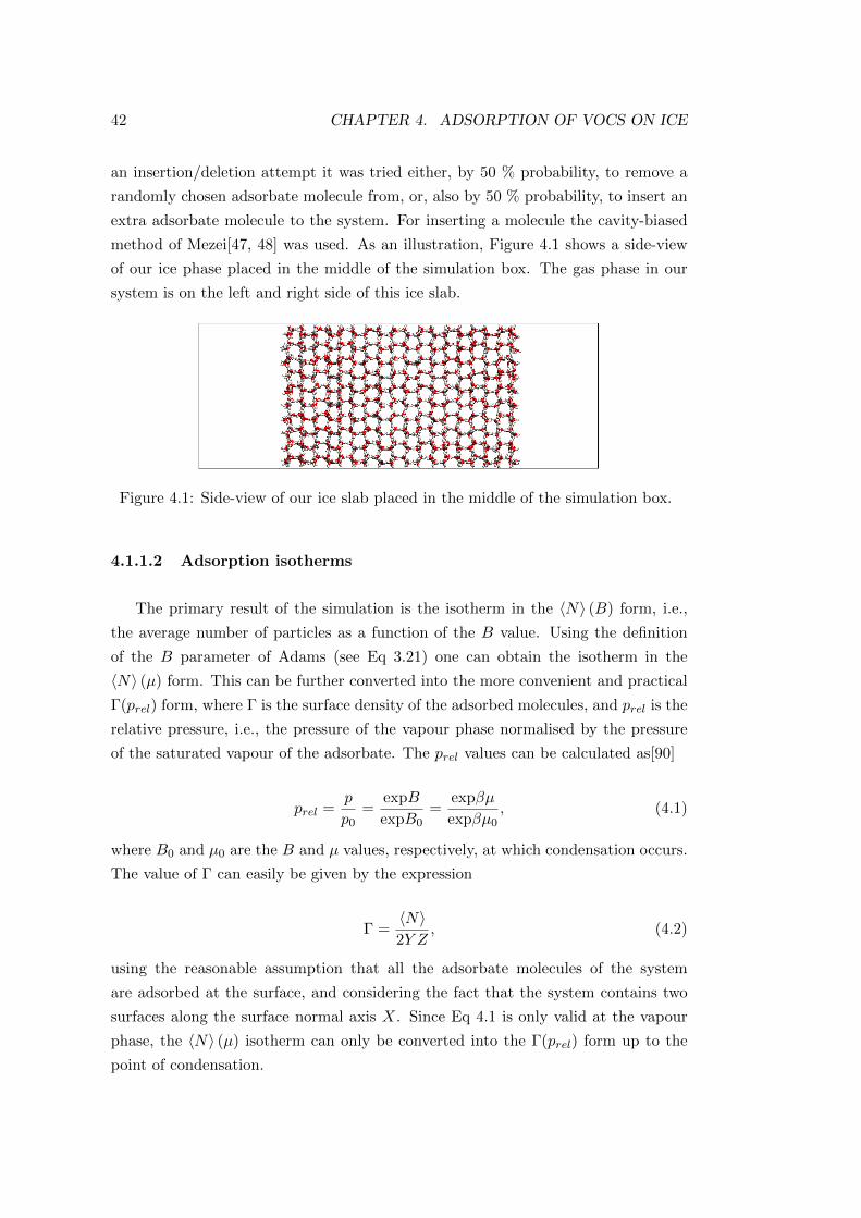
42 CHAPTER 4. ADSORPTION OF VOCS ON ICE
an insertion/deletion attempt it was tried either, by 50 % probability, to remove a
randomly chosen adsorbate molecule from, or, also by 50 % probability, to insert an
extra adsorbate molecule to the system. For inserting a molecule the cavity-biased
method of Mezei[47, 48] was used. As an illustration, Figure 4.1 shows a side-view
of our ice phase placed in the middle of the simulation box. The gas phase in our
system is on the left and right side of this ice slab.
Figure 4.1: Side-view of our ice slab placed in the middle of the simulation box.
4.1.1.2 Adsorption isotherms
The primary result of the simulation is the isotherm in the 〈N〉 (B) form, i.e.,
the average number of particles as a function of the B value. Using the definition
of the B parameter of Adams (see Eq 3.21) one can obtain the isotherm in the
〈N〉 (µ) form. This can be further converted into the more convenient and practical
Γ(prel) form, where Γ is the surface density of the adsorbed molecules, and prel is the
relative pressure, i.e., the pressure of the vapour phase normalised by the pressure
of the saturated vapour of the adsorbate. The prel values can be calculated as[90]
prel =p
p0=
expB
expB0=
expβµ
expβµ0, (4.1)
where B0 and µ0 are the B and µ values, respectively, at which condensation occurs.
The value of Γ can easily be given by the expression
Γ =〈N〉2Y Z
, (4.2)
using the reasonable assumption that all the adsorbate molecules of the system
are adsorbed at the surface, and considering the fact that the system contains two
surfaces along the surface normal axis X. Since Eq 4.1 is only valid at the vapour
phase, the 〈N〉 (µ) isotherm can only be converted into the Γ(prel) form up to the
point of condensation.
4.1. INTRODUCTION 43
The obtained isotherms in the Γ(prel) form can be adjusted using the Langmuir
isotherm:
Γ(prel) = ΓmaxprelK
1 + prelK, (4.3)
where the parameters Γmax and K are the saturated surface density and the par-
titioning coefficient between the solid and gas phase respectively. The Langmuir
theory assumes that i) all the adsorption sites are equivalent at the surface; ii) the
lateral interactions between the adsorbate molecules are negligible; and iii) no mul-
tilayer adsorption occurs. Another common choice in the analysis of the adsorption
isotherm is to use the Brunauer-Emmett-Teller (BET) theory[91]:
Γ(prel) =ΓmonoprelC
(1− prel) [1 + prel(C − 1)], (4.4)
where Γmono and C are the surface density of the saturated monolayer and the
BET coefficient respectively. The BET theory differs from the Langmuir model
by allowing multilayer adsorption, and hence it has to account for the interaction
between consecutive adsorption layers. However, lateral interactions within a given
layer are still neglected in this model. The C parameter is related to the energetics
of the adsorption:
C = exp∆Hout −∆H1
RT, (4.5)
where ∆H1 and ∆Hout are the enthalpies of adsorption in the first and subsequent
outer layers, respectively. The BET parameters Γmono and C are conventionally
determined by fitting the linearised form of the BET isotherm:
prelΓ(1− prel)
=1
ΓmonoC+C − 1
Γmonoprel. (4.6)
In practice, the data can be fitted by a straight line only in the 0.05 ≤ prel ≤ 0.35
range, thus one also has to limit the fitting procedure to this range.
4.1.1.3 Density profiles
To analyse the ordering of the adsorbate molecules along the surface normal
axis X one may calculate the number density profiles of the molecules. During
the calculation of this profile the simulation box is divided virtually into thin slices
along the surface normal axis X. In the collected configurations the number of the
44 CHAPTER 4. ADSORPTION OF VOCS ON ICE
molecules falling in each slice is counted, which is then normalised by the number
of configurations. The positions of the molecules are represented usually by that of
their central atom.
4.1.1.4 Interaction energy distribution
In order to characterise the energetic background of the adsorption process in the
simulation, the distribution of the total binding energy of the adsorbed molecules
UTOT (i.e., the interaction energy of a given adsorbate molecule with the rest of the
system) can be calculated, as well as the contributions coming from the interactions
with the ice phase U ice and with the other admolecules Uac, UFA and UBA in the
case of acetone, formic acid and benzaldehyde respectively.
4.1.1.5 Orientational analysis
The orientation of a rigid body relative to an external direction can be fully
described by two independent orientational variables. Therefore, the orientational
statistics of the molecules relative to a flat surface can only be given unambiguously
by the bivariate joint distribution of two such variables[92, 93]. Jedlovszky and
co-workers previously demonstrated that the polar angles ϑ and φ of the surface
normal vector in a local Cartesian frame fixed to the individual molecules represent
a suitable choice of these variables[92, 93].
Once the coordinate frame is defined in a reasonable way, the bivariate distribu-
tion functions can be calculated and plotted as maps using different tones to represent
different values. It should be noted that ϑ is the angle of two general spatial vectors,
but φ is formed by two vectors restricted to lie in a given plane by definition, and
hence uncorrelated orientation of the molecules with the surface results in a uniform
bivariate distribution only if cos ϑ and φ are chosen as independent variables.
4.2 Adsorption of acetone
4.2.1 Computational details of the simulations
Although several different potential models were proposed to describe acetone[96,
97, 98, 99, 100], the majority of these models are unable to capture the mixing proper-
ties of acetone with water[94, 95]. However, adsorbate – adsorbent interactions may
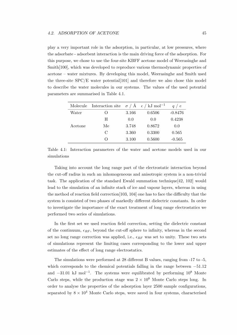
4.2. ADSORPTION OF ACETONE 45
play a very important role in the adsorption, in particular, at low pressures, where
the adsorbate - adsorbent interaction is the main driving force of the adsorption. For
this purpose, we chose to use the four-site KBFF acetone model of Weerasinghe and
Smith[100], which was developed to reproduce various thermodynamic properties of
acetone – water mixtures. By developing this model, Weerasinghe and Smith used
the three-site SPC/E water potential[101] and therefore we also chose this model
to describe the water molecules in our systems. The values of the used potential
parameters are summarised in Table 4.1.
Molecule Interaction site σ / A ε / kJ mol−1 q / e
Water O 3.166 0.6506 -0.8476
H 0.0 0.0 0.4238
Acetone Me 3.748 0.8672 0.0
C 3.360 0.3300 0.565
O 3.100 0.5600 -0.565
Table 4.1: Interaction parameters of the water and acetone models used in our
simulations
Taking into account the long range part of the electrostatic interaction beyond
the cut-off radius in such an inhomogeneous and anisotropic system is a non-trivial
task. The application of the standard Ewald summation technique[42, 102] would
lead to the simulation of an infinite stack of ice and vapour layers, whereas in using
the method of reaction field correction[103, 104] one has to face the difficulty that the
system is consisted of two phases of markedly different dielectric constants. In order
to investigate the importance of the exact treatment of long range electrostatics we
performed two series of simulations.
In the first set we used reaction field correction, setting the dielectric constant
of the continuum, εRF , beyond the cut-off sphere to infinity, whereas in the second
set no long range correction was applied, i.e., εRF was set to unity. These two sets
of simulations represent the limiting cases corresponding to the lower and upper
estimates of the effect of long range electrostatics.
The simulations were performed at 28 different B values, ranging from -17 to -5,
which corresponds to the chemical potentials falling in the range between −51.12
and −31.01 kJ mol−1. The systems were equilibrated by performing 108 Monte
Carlo steps, while the production stage was 2 × 10⁸ Monte Carlo steps long. In
order to analyse the properties of the adsorption layer 2500 sample configurations,
separated by 8 × 10⁴ Monte Carlo steps, were saved in four systems, characterised
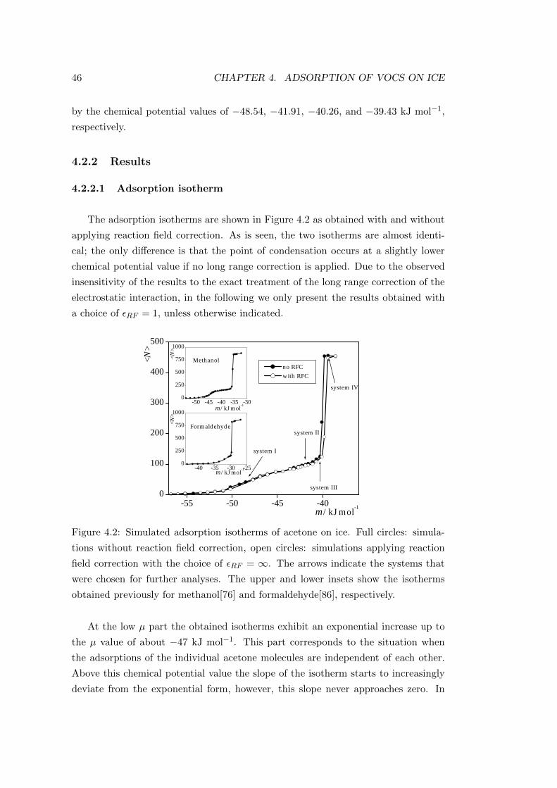
46 CHAPTER 4. ADSORPTION OF VOCS ON ICE
by the chemical potential values of −48.54, −41.91, −40.26, and −39.43 kJ mol−1,
respectively.
4.2.2 Results
4.2.2.1 Adsorption isotherm
The adsorption isotherms are shown in Figure 4.2 as obtained with and without
applying reaction field correction. As is seen, the two isotherms are almost identi-
cal; the only difference is that the point of condensation occurs at a slightly lower
chemical potential value if no long range correction is applied. Due to the observed
insensitivity of the results to the exact treatment of the long range correction of the
electrostatic interaction, in the following we only present the results obtained with
a choice of εRF = 1, unless otherwise indicated.
-55 -50 -45 -400
100
200
300
400
500
no RFC with RFC
system III
system I
system II
system IV
<N
>
µ / kJ mol-1
-50 -45 -40 -35 -300
250
500
750
1000
<N>
µ / kJ mol-1
Methanol
-40 -35 -30 -250
250
500
750
1000
<N>
µ / kJ mol-1
Formaldehyde
Figure 4.2: Simulated adsorption isotherms of acetone on ice. Full circles: simula-
tions without reaction field correction, open circles: simulations applying reaction
field correction with the choice of εRF = ∞. The arrows indicate the systems that
were chosen for further analyses. The upper and lower insets show the isotherms
obtained previously for methanol[76] and formaldehyde[86], respectively.
At the low µ part the obtained isotherms exhibit an exponential increase up to
the µ value of about −47 kJ mol−1. This part corresponds to the situation when
the adsorptions of the individual acetone molecules are independent of each other.
Above this chemical potential value the slope of the isotherm starts to increasingly
deviate from the exponential form, however, this slope never approaches zero. In
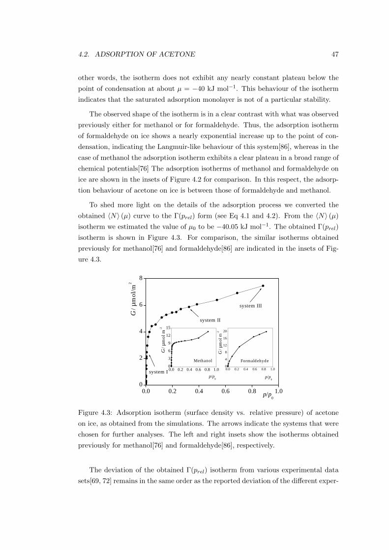
4.2. ADSORPTION OF ACETONE 47
other words, the isotherm does not exhibit any nearly constant plateau below the
point of condensation at about µ = −40 kJ mol−1. This behaviour of the isotherm
indicates that the saturated adsorption monolayer is not of a particular stability.
The observed shape of the isotherm is in a clear contrast with what was observed
previously either for methanol or for formaldehyde. Thus, the adsorption isotherm
of formaldehyde on ice shows a nearly exponential increase up to the point of con-
densation, indicating the Langmuir-like behaviour of this system[86], whereas in the
case of methanol the adsorption isotherm exhibits a clear plateau in a broad range of
chemical potentials[76] The adsorption isotherms of methanol and formaldehyde on
ice are shown in the insets of Figure 4.2 for comparison. In this respect, the adsorp-
tion behaviour of acetone on ice is between those of formaldehyde and methanol.
To shed more light on the details of the adsorption process we converted the
obtained 〈N〉 (µ) curve to the Γ(prel) form (see Eq 4.1 and 4.2). From the 〈N〉 (µ)
isotherm we estimated the value of µ0 to be −40.05 kJ mol−1. The obtained Γ(prel)
isotherm is shown in Figure 4.3. For comparison, the similar isotherms obtained
previously for methanol[76] and formaldehyde[86] are indicated in the insets of Fig-
ure 4.3.
0.0 0.2 0.4 0.6 0.8 1.00
2
4
6
8
system III
system II
system I
Γ / µ
mol
/m2
p/p0
0.0 0.2 0.4 0.6 0.8 1.00
3
6
9
12
15
Methanol
p/p0
Γ / µ
mol
m-2
0.0 0.2 0.4 0.6 0.8 1.00
4
8
12
16
20
Formaldehyde
p/p0
Γ / µ
mol
m-2
Figure 4.3: Adsorption isotherm (surface density vs. relative pressure) of acetone
on ice, as obtained from the simulations. The arrows indicate the systems that were
chosen for further analyses. The left and right insets show the isotherms obtained
previously for methanol[76] and formaldehyde[86], respectively.
The deviation of the obtained Γ(prel) isotherm from various experimental data
sets[69, 72] remains in the same order as the reported deviation of the different exper-
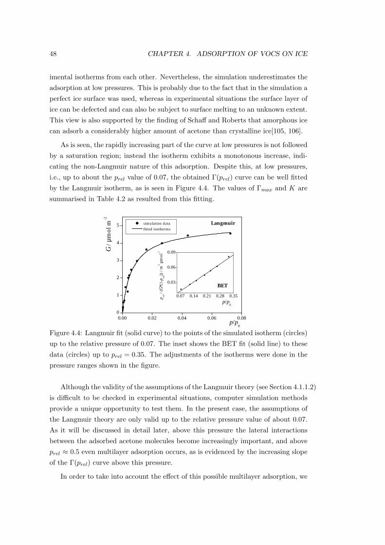
48 CHAPTER 4. ADSORPTION OF VOCS ON ICE
imental isotherms from each other. Nevertheless, the simulation underestimates the
adsorption at low pressures. This is probably due to the fact that in the simulation a
perfect ice surface was used, whereas in experimental situations the surface layer of
ice can be defected and can also be subject to surface melting to an unknown extent.
This view is also supported by the finding of Schaff and Roberts that amorphous ice
can adsorb a considerably higher amount of acetone than crystalline ice[105, 106].
As is seen, the rapidly increasing part of the curve at low pressures is not followed
by a saturation region; instead the isotherm exhibits a monotonous increase, indi-
cating the non-Langmuir nature of this adsorption. Despite this, at low pressures,
i.e., up to about the prel value of 0.07, the obtained Γ(prel) curve can be well fitted
by the Langmuir isotherm, as is seen in Figure 4.4. The values of Γmax and K are
summarised in Table 4.2 as resulted from this fitting.
0.00 0.02 0.04 0.06 0.080
1
2
3
4
5
0.07 0.14 0.21 0.28 0.35
0.03
0.06
0.09
BET
Langmuir simulation data fitted isotherms
p rel /
(Γ*(
1-p re
l)) /
m2 µ
mol
-1
p/p0
Γ / µ
mol
m-2
p/p0
Figure 4.4: Langmuir fit (solid curve) to the points of the simulated isotherm (circles)
up to the relative pressure of 0.07. The inset shows the BET fit (solid line) to these
data (circles) up to prel = 0.35. The adjustments of the isotherms were done in the
pressure ranges shown in the figure.
Although the validity of the assumptions of the Langmuir theory (see Section 4.1.1.2)
is difficult to be checked in experimental situations, computer simulation methods
provide a unique opportunity to test them. In the present case, the assumptions of
the Langmuir theory are only valid up to the relative pressure value of about 0.07.
As it will be discussed in detail later, above this pressure the lateral interactions
between the adsorbed acetone molecules become increasingly important, and above
prel ≈ 0.5 even multilayer adsorption occurs, as is evidenced by the increasing slope
of the Γ(prel) curve above this pressure.
In order to take into account the effect of this possible multilayer adsorption, we
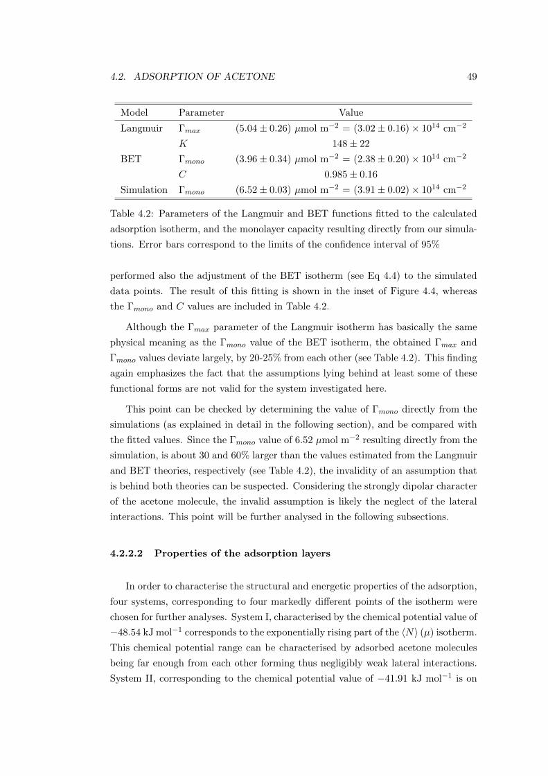
4.2. ADSORPTION OF ACETONE 49
Model Parameter Value
Langmuir Γmax (5.04± 0.26) µmol m−2 = (3.02± 0.16)× 1014 cm−2
K 148± 22
BET Γmono (3.96± 0.34) µmol m−2 = (2.38± 0.20)× 1014 cm−2
C 0.985± 0.16
Simulation Γmono (6.52± 0.03) µmol m−2 = (3.91± 0.02)× 1014 cm−2
Table 4.2: Parameters of the Langmuir and BET functions fitted to the calculated
adsorption isotherm, and the monolayer capacity resulting directly from our simula-
tions. Error bars correspond to the limits of the confidence interval of 95%
performed also the adjustment of the BET isotherm (see Eq 4.4) to the simulated
data points. The result of this fitting is shown in the inset of Figure 4.4, whereas
the Γmono and C values are included in Table 4.2.
Although the Γmax parameter of the Langmuir isotherm has basically the same
physical meaning as the Γmono value of the BET isotherm, the obtained Γmax and
Γmono values deviate largely, by 20-25% from each other (see Table 4.2). This finding
again emphasizes the fact that the assumptions lying behind at least some of these
functional forms are not valid for the system investigated here.
This point can be checked by determining the value of Γmono directly from the
simulations (as explained in detail in the following section), and be compared with
the fitted values. Since the Γmono value of 6.52 µmol m−2 resulting directly from the
simulation, is about 30 and 60% larger than the values estimated from the Langmuir
and BET theories, respectively (see Table 4.2), the invalidity of an assumption that
is behind both theories can be suspected. Considering the strongly dipolar character
of the acetone molecule, the invalid assumption is likely the neglect of the lateral
interactions. This point will be further analysed in the following subsections.
4.2.2.2 Properties of the adsorption layers
In order to characterise the structural and energetic properties of the adsorption,
four systems, corresponding to four markedly different points of the isotherm were
chosen for further analyses. System I, characterised by the chemical potential value of
−48.54 kJ mol−1 corresponds to the exponentially rising part of the 〈N〉 (µ) isotherm.
This chemical potential range can be characterised by adsorbed acetone molecules
being far enough from each other forming thus negligibly weak lateral interactions.
System II, corresponding to the chemical potential value of −41.91 kJ mol−1 is on
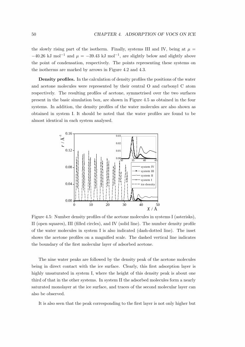
50 CHAPTER 4. ADSORPTION OF VOCS ON ICE
the slowly rising part of the isotherm. Finally, systems III and IV, being at µ =
−40.26 kJ mol−1 and µ = −39.43 kJ mol−1, are slightly below and slightly above
the point of condensation, respectively. The points representing these systems on
the isotherms are marked by arrows in Figure 4.2 and 4.3.
Density profiles. In the calculation of density profiles the positions of the water
and acetone molecules were represented by their central O and carbonyl C atom
respectively. The resulting profiles of acetone, symmetrised over the two surfaces
present in the basic simulation box, are shown in Figure 4.5 as obtained in the four
systems. In addition, the density profiles of the water molecules are also shown as
obtained in system I. It should be noted that the water profiles are found to be
almost identical in each system analysed.
0 10 20 30 40 500.00
0.04
0.08
0.12
0.16
30 35 40 450.00
0.01
0.02
0.03
ρ / Å
-3
X / Å
system IV system III system II system I ice density
Figure 4.5: Number density profiles of the acetone molecules in systems I (asterisks),
II (open squares), III (filled circles), and IV (solid line). The number density profile
of the water molecules in system I is also indicated (dash-dotted line). The inset
shows the acetone profiles on a magnified scale. The dashed vertical line indicates
the boundary of the first molecular layer of adsorbed acetone.
The nine water peaks are followed by the density peak of the acetone molecules
being in direct contact with the ice surface. Clearly, this first adsorption layer is
highly unsaturated in system I, where the height of this density peak is about one
third of that in the other systems. In system II the adsorbed molecules form a nearly
saturated monolayer at the ice surface, and traces of the second molecular layer can
also be observed.
It is also seen that the peak corresponding to the first layer is not only higher but
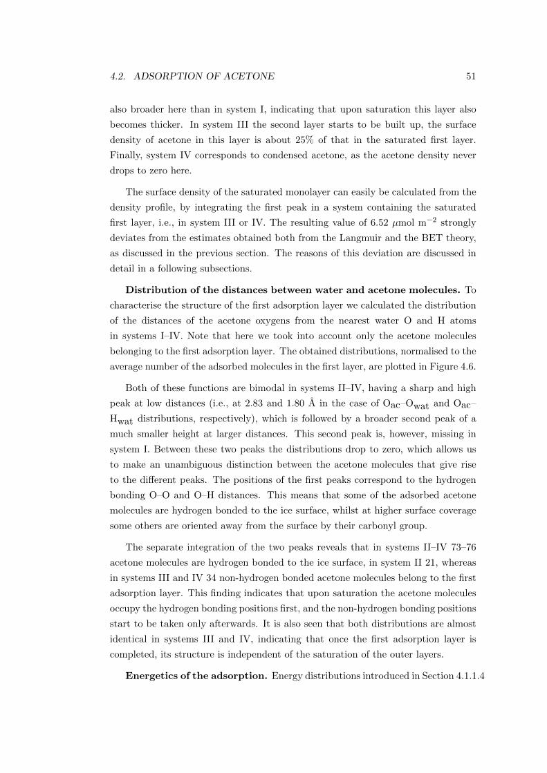
4.2. ADSORPTION OF ACETONE 51
also broader here than in system I, indicating that upon saturation this layer also
becomes thicker. In system III the second layer starts to be built up, the surface
density of acetone in this layer is about 25% of that in the saturated first layer.
Finally, system IV corresponds to condensed acetone, as the acetone density never
drops to zero here.
The surface density of the saturated monolayer can easily be calculated from the
density profile, by integrating the first peak in a system containing the saturated
first layer, i.e., in system III or IV. The resulting value of 6.52 µmol m−2 strongly
deviates from the estimates obtained both from the Langmuir and the BET theory,
as discussed in the previous section. The reasons of this deviation are discussed in
detail in a following subsections.
Distribution of the distances between water and acetone molecules. To
characterise the structure of the first adsorption layer we calculated the distribution
of the distances of the acetone oxygens from the nearest water O and H atoms
in systems I–IV. Note that here we took into account only the acetone molecules
belonging to the first adsorption layer. The obtained distributions, normalised to the
average number of the adsorbed molecules in the first layer, are plotted in Figure 4.6.
Both of these functions are bimodal in systems II–IV, having a sharp and high
peak at low distances (i.e., at 2.83 and 1.80 A in the case of Oac–Owat and Oac–
Hwat distributions, respectively), which is followed by a broader second peak of a
much smaller height at larger distances. This second peak is, however, missing in
system I. Between these two peaks the distributions drop to zero, which allows us
to make an unambiguous distinction between the acetone molecules that give rise
to the different peaks. The positions of the first peaks correspond to the hydrogen
bonding O–O and O–H distances. This means that some of the adsorbed acetone
molecules are hydrogen bonded to the ice surface, whilst at higher surface coverage
some others are oriented away from the surface by their carbonyl group.
The separate integration of the two peaks reveals that in systems II–IV 73–76
acetone molecules are hydrogen bonded to the ice surface, in system II 21, whereas
in systems III and IV 34 non-hydrogen bonded acetone molecules belong to the first
adsorption layer. This finding indicates that upon saturation the acetone molecules
occupy the hydrogen bonding positions first, and the non-hydrogen bonding positions
start to be taken only afterwards. It is also seen that both distributions are almost
identical in systems III and IV, indicating that once the first adsorption layer is
completed, its structure is independent of the saturation of the outer layers.
Energetics of the adsorption. Energy distributions introduced in Section 4.1.1.4
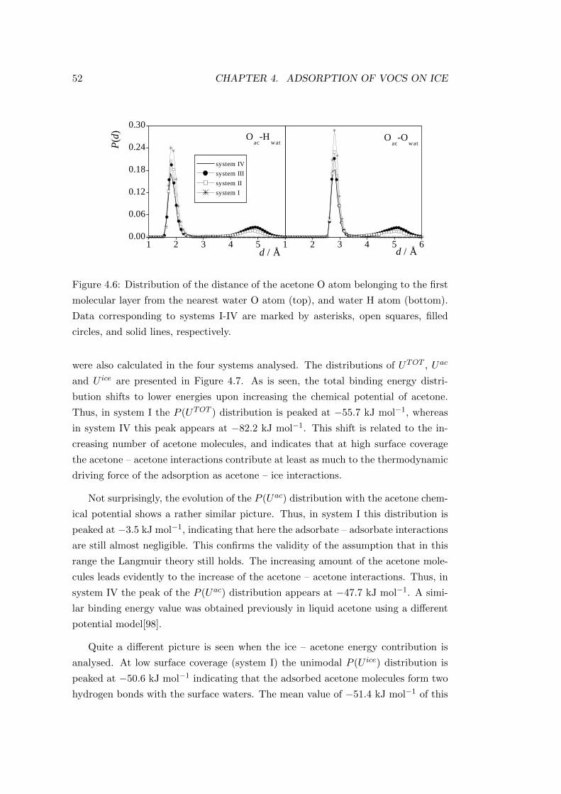
52 CHAPTER 4. ADSORPTION OF VOCS ON ICE
1 2 3 4 50.00
0.06
0.12
0.18
0.24
0.30
1 2 3 4 5 6d / Å
Oac
-Hwat
P(
d)
d / Å
system IV system III system II system I
Oac
-Owat
Figure 4.6: Distribution of the distance of the acetone O atom belonging to the first
molecular layer from the nearest water O atom (top), and water H atom (bottom).
Data corresponding to systems I-IV are marked by asterisks, open squares, filled
circles, and solid lines, respectively.
were also calculated in the four systems analysed. The distributions of UTOT , Uac
and U ice are presented in Figure 4.7. As is seen, the total binding energy distri-
bution shifts to lower energies upon increasing the chemical potential of acetone.
Thus, in system I the P (UTOT ) distribution is peaked at −55.7 kJ mol−1, whereas
in system IV this peak appears at −82.2 kJ mol−1. This shift is related to the in-
creasing number of acetone molecules, and indicates that at high surface coverage
the acetone – acetone interactions contribute at least as much to the thermodynamic
driving force of the adsorption as acetone – ice interactions.
Not surprisingly, the evolution of the P (Uac) distribution with the acetone chem-
ical potential shows a rather similar picture. Thus, in system I this distribution is
peaked at −3.5 kJ mol−1, indicating that here the adsorbate – adsorbate interactions
are still almost negligible. This confirms the validity of the assumption that in this
range the Langmuir theory still holds. The increasing amount of the acetone mole-
cules leads evidently to the increase of the acetone – acetone interactions. Thus, in
system IV the peak of the P (Uac) distribution appears at −47.7 kJ mol−1. A simi-
lar binding energy value was obtained previously in liquid acetone using a different
potential model[98].
Quite a different picture is seen when the ice – acetone energy contribution is
analysed. At low surface coverage (system I) the unimodal P (U ice) distribution is
peaked at −50.6 kJ mol−1 indicating that the adsorbed acetone molecules form two
hydrogen bonds with the surface waters. The mean value of −51.4 kJ mol−1 of this
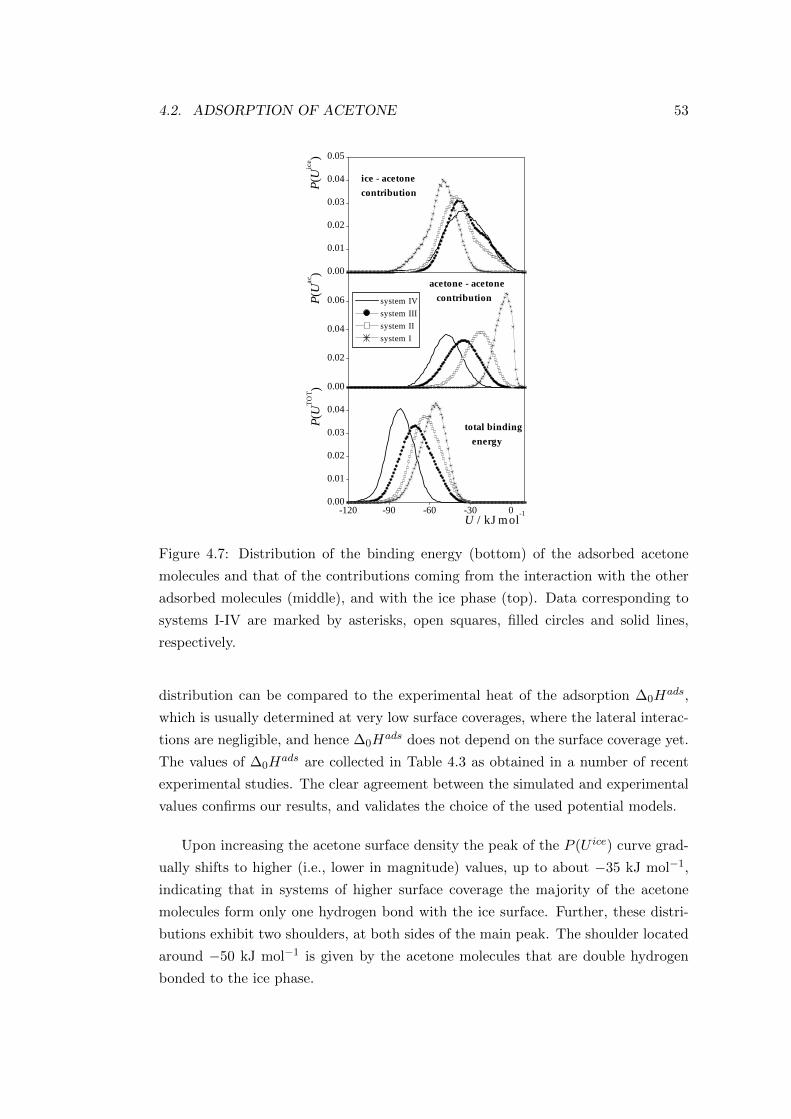
4.2. ADSORPTION OF ACETONE 53
-120 -90 -60 -30 00.00
0.01
0.02
0.03
0.04
0.00
0.02
0.04
0.06
0.00
0.01
0.02
0.03
0.04
0.05
total binding energy
P(U
ice )
P(U
TOT )
system IV system III system II system I
U / kJ mol-1
P(U
ac)
acetone - acetone contribution
ice - acetone contribution
Figure 4.7: Distribution of the binding energy (bottom) of the adsorbed acetone
molecules and that of the contributions coming from the interaction with the other
adsorbed molecules (middle), and with the ice phase (top). Data corresponding to
systems I-IV are marked by asterisks, open squares, filled circles and solid lines,
respectively.
distribution can be compared to the experimental heat of the adsorption ∆0Hads,
which is usually determined at very low surface coverages, where the lateral interac-
tions are negligible, and hence ∆0Hads does not depend on the surface coverage yet.
The values of ∆0Hads are collected in Table 4.3 as obtained in a number of recent
experimental studies. The clear agreement between the simulated and experimental
values confirms our results, and validates the choice of the used potential models.
Upon increasing the acetone surface density the peak of the P (U ice) curve grad-
ually shifts to higher (i.e., lower in magnitude) values, up to about −35 kJ mol−1,
indicating that in systems of higher surface coverage the majority of the acetone
molecules form only one hydrogen bond with the ice surface. Further, these distri-
butions exhibit two shoulders, at both sides of the main peak. The shoulder located
around −50 kJ mol−1 is given by the acetone molecules that are double hydrogen
bonded to the ice phase.
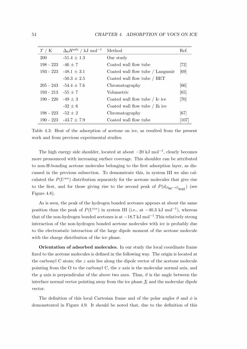
54 CHAPTER 4. ADSORPTION OF VOCS ON ICE
T / K ∆0Hads / kJ mol−1 Method Ref.
200 -51.4 ± 1.3 Our study
198 - 223 -46 ± 7 Coated wall flow tube [72]
193 - 223 -48.1 ± 3.1 Coated wall flow tube / Langmuir [69]
-50.3 ± 2.5 Coated wall flow tube / BET
205 - 243 -54.4 ± 7.6 Chromatography [66]
193 - 213 -55 ± 7 Volumetric [65]
190 - 220 -49 ± 3 Coated wall flow tube / Ic ice [70]
-32 ± 6 Coated wall flow tube / Ih ice
198 - 223 -52 ± 2 Chromatography [67]
190 - 223 -43.7 ± 7.9 Coated wall flow tube [107]
Table 4.3: Heat of the adsorption of acetone on ice, as resulted from the present
work and from previous experimental studies.
The high energy side shoulder, located at about −20 kJ mol−1, clearly becomes
more pronounced with increasing surface coverage. This shoulder can be attributed
to non-H-bonding acetone molecules belonging to the first adsorption layer, as dis-
cussed in the previous subsection. To demonstrate this, in system III we also cal-
culated the P (U ice) distribution separately for the acetone molecules that give rise
to the first, and for those giving rise to the second peak of P (dOac−Owat) (see
Figure 4.8).
As is seen, the peak of the hydrogen bonded acetones appears at about the same
position than the peak of P (U ice) in system III (i.e., at −40.3 kJ mol−1), whereas
that of the non-hydrogen bonded acetones is at −18.7 kJ mol−1.This relatively strong
interaction of the non-hydrogen bonded acetone molecules with ice is probably due
to the electrostatic interaction of the large dipole moment of the acetone molecule
with the charge distribution of the ice phase.
Orientation of adsorbed molecules. In our study the local coordinate frame
fixed to the acetone molecules is defined in the following way. The origin is located at
the carbonyl C atom; the z axis lies along the dipole vector of the acetone molecule
pointing from the O to the carbonyl C, the x axis is the molecular normal axis, and
the y axis is perpendicular of the above two axes. Thus, ϑ is the angle between the
interface normal vector pointing away from the ice phase X and the molecular dipole
vector.
The definition of this local Cartesian frame and of the polar angles ϑ and φ is
demonstrated in Figure 4.9. It should be noted that, due to the definition of this
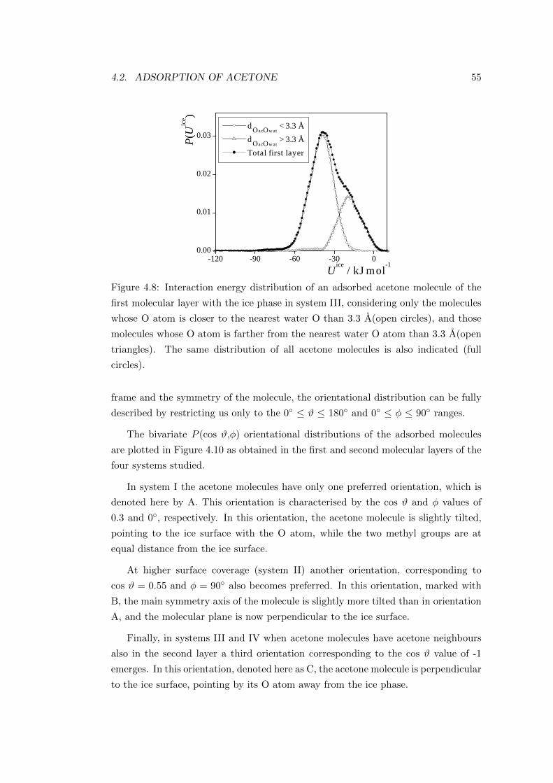
4.2. ADSORPTION OF ACETONE 55
-120 -90 -60 -30 00.00
0.01
0.02
0.03
dOacOwat < 3.3 Å
dOacOwat > 3.3 Å
Total first layer
P(U
ice )
Uice / kJ mol-1
Figure 4.8: Interaction energy distribution of an adsorbed acetone molecule of the
first molecular layer with the ice phase in system III, considering only the molecules
whose O atom is closer to the nearest water O than 3.3 A(open circles), and those
molecules whose O atom is farther from the nearest water O atom than 3.3 A(open
triangles). The same distribution of all acetone molecules is also indicated (full
circles).
frame and the symmetry of the molecule, the orientational distribution can be fully
described by restricting us only to the 0 ≤ ϑ ≤ 180 and 0 ≤ φ ≤ 90 ranges.
The bivariate P (cos ϑ,φ) orientational distributions of the adsorbed molecules
are plotted in Figure 4.10 as obtained in the first and second molecular layers of the
four systems studied.
In system I the acetone molecules have only one preferred orientation, which is
denoted here by A. This orientation is characterised by the cos ϑ and φ values of
0.3 and 0, respectively. In this orientation, the acetone molecule is slightly tilted,
pointing to the ice surface with the O atom, while the two methyl groups are at
equal distance from the ice surface.
At higher surface coverage (system II) another orientation, corresponding to
cos ϑ = 0.55 and φ = 90 also becomes preferred. In this orientation, marked with
B, the main symmetry axis of the molecule is slightly more tilted than in orientation
A, and the molecular plane is now perpendicular to the ice surface.
Finally, in systems III and IV when acetone molecules have acetone neighbours
also in the second layer a third orientation corresponding to the cos ϑ value of -1
emerges. In this orientation, denoted here as C, the acetone molecule is perpendicular
to the ice surface, pointing by its O atom away from the ice phase.
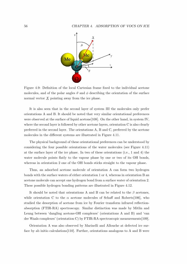
56 CHAPTER 4. ADSORPTION OF VOCS ON ICE
Figure 4.9: Definition of the local Cartesian frame fixed to the individual acetone
molecules, and of the polar angles ϑ and φ describing the orientation of the surface
normal vector X pointing away from the ice phase.
It is also seen that in the second layer of system III the molecules only prefer
orientations A and B. It should be noted that very similar orientational preferences
were observed at the surface of liquid acetone[108]. On the other hand, in system IV,
where the second layer is followed by other acetone layers, orientation C is also clearly
preferred in the second layer. The orientations A, B and C, preferred by the acetone
molecules in the different systems are illustrated in Figure 4.11.
The physical background of these orientational preferences can be understood by
considering the four possible orientations of the water molecules (see Figure 4.11)
at the surface layer of the ice phase. In two of these orientations (i.e., 1 and 4) the
water molecule points flatly to the vapour phase by one or two of its OH bonds,
whereas in orientation 2 one of the OH bonds sticks straight to the vapour phase.
Thus, an adsorbed acetone molecule of orientation A can form two hydrogen
bonds with the surface waters of either orientation 1 or 4, whereas in orientation B an
acetone molecule can accept one hydrogen bond from a surface water of orientation 2.
These possible hydrogen bonding patterns are illustrated in Figure 4.12.
It should be noted that orientations A and B can be related to the β acetones,
while orientation C to the α acetone molecules of Schaff and Roberts[106], who
studied the desorption of acetone from ice by Fourier transform infrared reflection-
absorption (FTIR-RA) spectroscopy. Similar distinction was made by Mitlin and
Leung between ‘dangling acetone-OH complexes’ (orientations A and B) and ‘van
der Waals complexes’ (orientation C) by FTIR-RA spectroscopic measurements[109].
Orientation A was also observed by Marinelli and Allouche at defected ice sur-
face by ab initio calculations[110]. Further, orientations analogous to A and B were
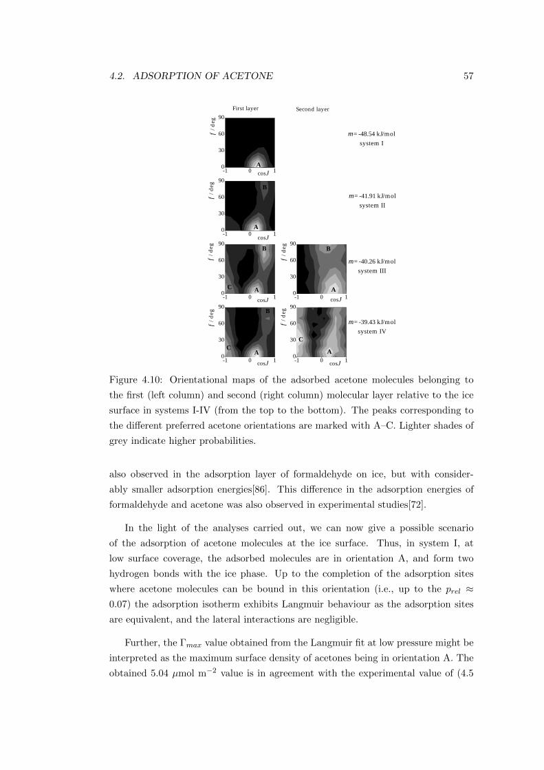
4.2. ADSORPTION OF ACETONE 57
-1 0 10
30
60
90
-1 0 10
30
60
90
-1 0 10
30
60
90-1 0 1
0
30
60
90
-1 0 10
30
60
90
-1 0 10
30
60
90
B
First layer Second layer
C
CC
B
BB
A
AA
A
A
Acosϑ
φ / d
egφ
/ deg
µ = -48.54 kJ/molsystem I
µ = -41.91 kJ/molsystem II
µ = -40.26 kJ/molsystem III
µ = -39.43 kJ/molsystem IV
φ / d
egφ
/ deg
φ / d
egφ
/ deg
cosϑ
cosϑ cosϑ
cosϑ
cosϑ
Figure 4.10: Orientational maps of the adsorbed acetone molecules belonging to
the first (left column) and second (right column) molecular layer relative to the ice
surface in systems I-IV (from the top to the bottom). The peaks corresponding to
the different preferred acetone orientations are marked with A–C. Lighter shades of
grey indicate higher probabilities.
also observed in the adsorption layer of formaldehyde on ice, but with consider-
ably smaller adsorption energies[86]. This difference in the adsorption energies of
formaldehyde and acetone was also observed in experimental studies[72].
In the light of the analyses carried out, we can now give a possible scenario
of the adsorption of acetone molecules at the ice surface. Thus, in system I, at
low surface coverage, the adsorbed molecules are in orientation A, and form two
hydrogen bonds with the ice phase. Up to the completion of the adsorption sites
where acetone molecules can be bound in this orientation (i.e., up to the prel ≈0.07) the adsorption isotherm exhibits Langmuir behaviour as the adsorption sites
are equivalent, and the lateral interactions are negligible.
Further, the Γmax value obtained from the Langmuir fit at low pressure might be
interpreted as the maximum surface density of acetones being in orientation A. The
obtained 5.04 µmol m−2 value is in agreement with the experimental value of (4.5
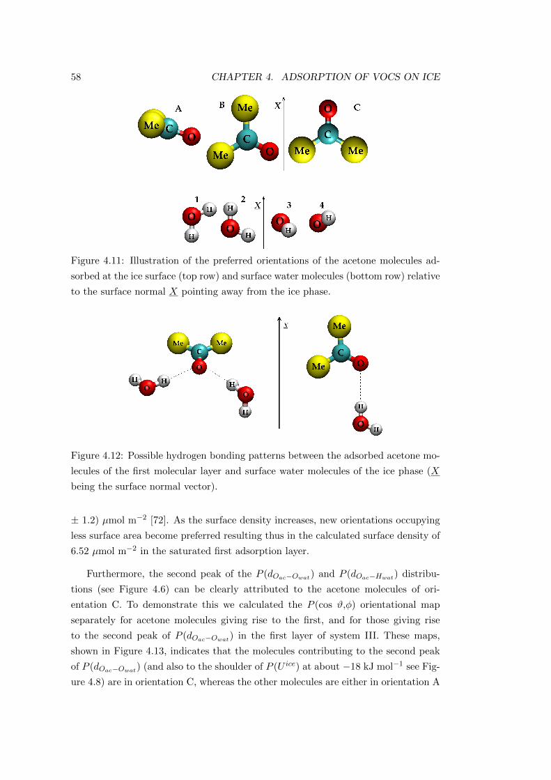
58 CHAPTER 4. ADSORPTION OF VOCS ON ICE
Figure 4.11: Illustration of the preferred orientations of the acetone molecules ad-
sorbed at the ice surface (top row) and surface water molecules (bottom row) relative
to the surface normal X pointing away from the ice phase.
Figure 4.12: Possible hydrogen bonding patterns between the adsorbed acetone mo-
lecules of the first molecular layer and surface water molecules of the ice phase (X
being the surface normal vector).
± 1.2) µmol m−2 [72]. As the surface density increases, new orientations occupying
less surface area become preferred resulting thus in the calculated surface density of
6.52 µmol m−2 in the saturated first adsorption layer.
Furthermore, the second peak of the P (dOac−Owat) and P (dOac−Hwat) distribu-
tions (see Figure 4.6) can be clearly attributed to the acetone molecules of ori-
entation C. To demonstrate this we calculated the P (cos ϑ,φ) orientational map
separately for acetone molecules giving rise to the first, and for those giving rise
to the second peak of P (dOac−Owat) in the first layer of system III. These maps,
shown in Figure 4.13, indicates that the molecules contributing to the second peak
of P (dOac−Owat) (and also to the shoulder of P (U ice) at about −18 kJ mol−1 see Fig-
ure 4.8) are in orientation C, whereas the other molecules are either in orientation A
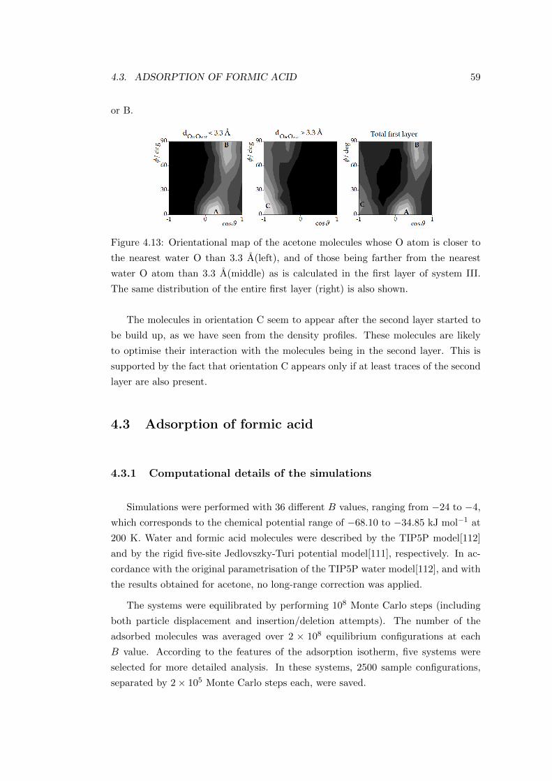
4.3. ADSORPTION OF FORMIC ACID 59
or B.
Figure 4.13: Orientational map of the acetone molecules whose O atom is closer to
the nearest water O than 3.3 A(left), and of those being farther from the nearest
water O atom than 3.3 A(middle) as is calculated in the first layer of system III.
The same distribution of the entire first layer (right) is also shown.
The molecules in orientation C seem to appear after the second layer started to
be build up, as we have seen from the density profiles. These molecules are likely
to optimise their interaction with the molecules being in the second layer. This is
supported by the fact that orientation C appears only if at least traces of the second
layer are also present.
4.3 Adsorption of formic acid
4.3.1 Computational details of the simulations
Simulations were performed with 36 different B values, ranging from −24 to −4,
which corresponds to the chemical potential range of −68.10 to −34.85 kJ mol−1 at
200 K. Water and formic acid molecules were described by the TIP5P model[112]
and by the rigid five-site Jedlovszky-Turi potential model[111], respectively. In ac-
cordance with the original parametrisation of the TIP5P water model[112], and with
the results obtained for acetone, no long-range correction was applied.
The systems were equilibrated by performing 108 Monte Carlo steps (including
both particle displacement and insertion/deletion attempts). The number of the
adsorbed molecules was averaged over 2 × 10⁸ equilibrium configurations at each
B value. According to the features of the adsorption isotherm, five systems were
selected for more detailed analysis. In these systems, 2500 sample configurations,
separated by 2× 10⁵ Monte Carlo steps each, were saved.
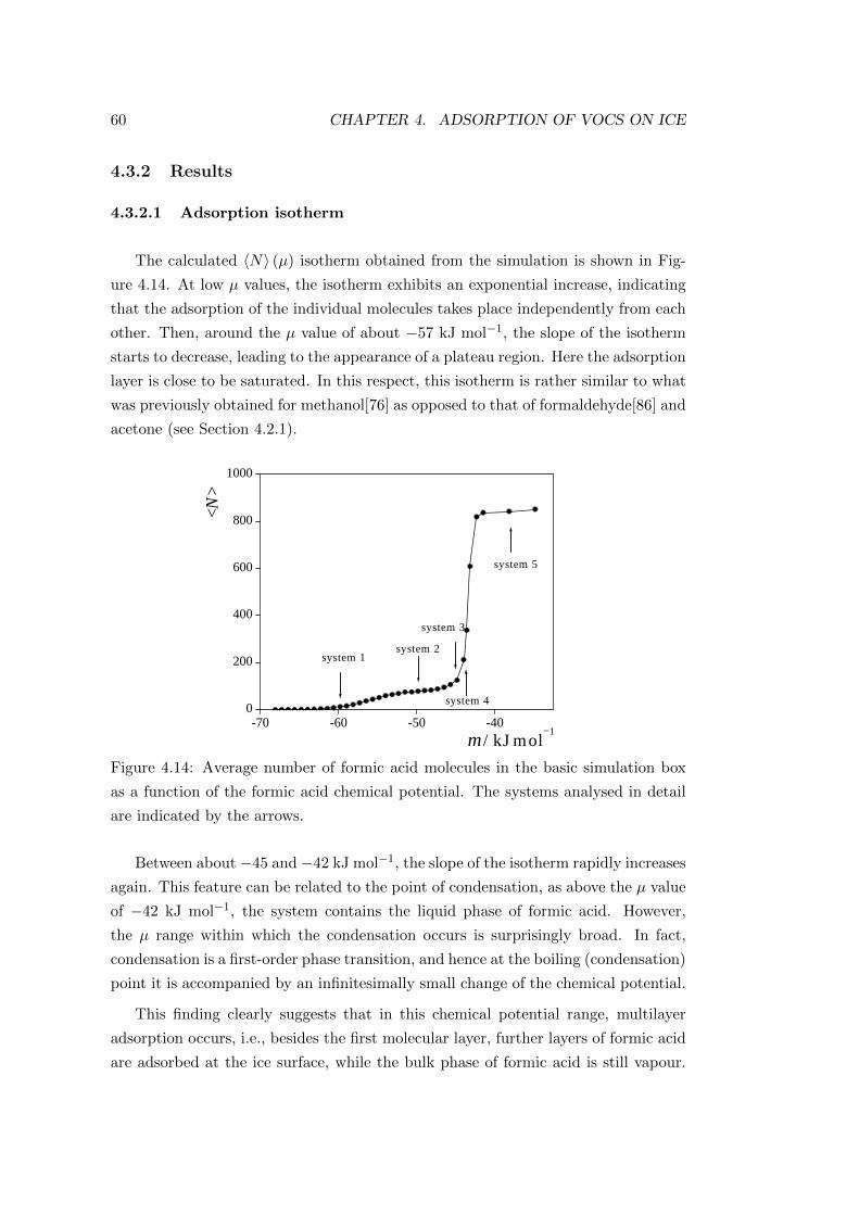
60 CHAPTER 4. ADSORPTION OF VOCS ON ICE
4.3.2 Results
4.3.2.1 Adsorption isotherm
The calculated 〈N〉 (µ) isotherm obtained from the simulation is shown in Fig-
ure 4.14. At low µ values, the isotherm exhibits an exponential increase, indicating
that the adsorption of the individual molecules takes place independently from each
other. Then, around the µ value of about −57 kJ mol−1, the slope of the isotherm
starts to decrease, leading to the appearance of a plateau region. Here the adsorption
layer is close to be saturated. In this respect, this isotherm is rather similar to what
was previously obtained for methanol[76] as opposed to that of formaldehyde[86] and
acetone (see Section 4.2.1).
-70 -60 -50 -400
200
400
600
800
1000
system 5
system 4
system 3
system 2system 1
<N>
µ / kJ mol−1
Figure 4.14: Average number of formic acid molecules in the basic simulation box
as a function of the formic acid chemical potential. The systems analysed in detail
are indicated by the arrows.
Between about −45 and −42 kJ mol−1, the slope of the isotherm rapidly increases
again. This feature can be related to the point of condensation, as above the µ value
of −42 kJ mol−1, the system contains the liquid phase of formic acid. However,
the µ range within which the condensation occurs is surprisingly broad. In fact,
condensation is a first-order phase transition, and hence at the boiling (condensation)
point it is accompanied by an infinitesimally small change of the chemical potential.
This finding clearly suggests that in this chemical potential range, multilayer
adsorption occurs, i.e., besides the first molecular layer, further layers of formic acid
are adsorbed at the ice surface, while the bulk phase of formic acid is still vapour.
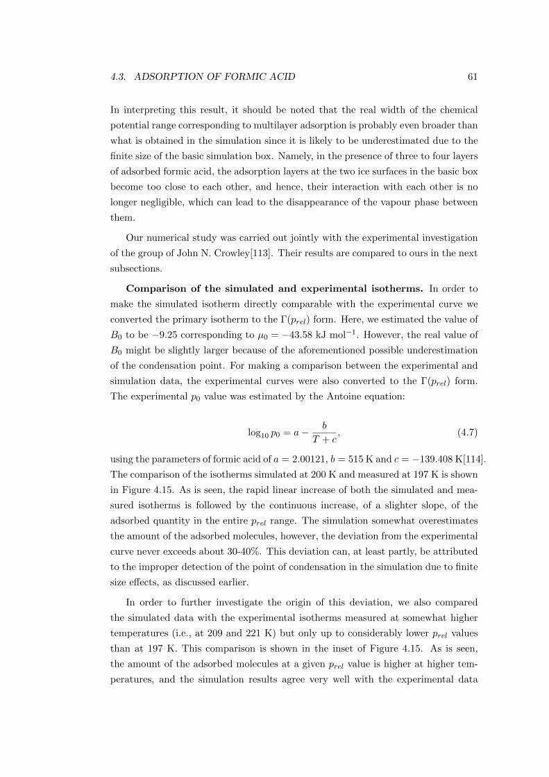
4.3. ADSORPTION OF FORMIC ACID 61
In interpreting this result, it should be noted that the real width of the chemical
potential range corresponding to multilayer adsorption is probably even broader than
what is obtained in the simulation since it is likely to be underestimated due to the
finite size of the basic simulation box. Namely, in the presence of three to four layers
of adsorbed formic acid, the adsorption layers at the two ice surfaces in the basic box
become too close to each other, and hence, their interaction with each other is no
longer negligible, which can lead to the disappearance of the vapour phase between
them.
Our numerical study was carried out jointly with the experimental investigation
of the group of John N. Crowley[113]. Their results are compared to ours in the next
subsections.
Comparison of the simulated and experimental isotherms. In order to
make the simulated isotherm directly comparable with the experimental curve we
converted the primary isotherm to the Γ(prel) form. Here, we estimated the value of
B0 to be −9.25 corresponding to µ0 = −43.58 kJ mol−1. However, the real value of
B0 might be slightly larger because of the aforementioned possible underestimation
of the condensation point. For making a comparison between the experimental and
simulation data, the experimental curves were also converted to the Γ(prel) form.
The experimental p0 value was estimated by the Antoine equation:
log10 p0 = a− b
T + c, (4.7)
using the parameters of formic acid of a = 2.00121, b = 515 K and c = −139.408 K[114].
The comparison of the isotherms simulated at 200 K and measured at 197 K is shown
in Figure 4.15. As is seen, the rapid linear increase of both the simulated and mea-
sured isotherms is followed by the continuous increase, of a slighter slope, of the
adsorbed quantity in the entire prel range. The simulation somewhat overestimates
the amount of the adsorbed molecules, however, the deviation from the experimental
curve never exceeds about 30-40%. This deviation can, at least partly, be attributed
to the improper detection of the point of condensation in the simulation due to finite
size effects, as discussed earlier.
In order to further investigate the origin of this deviation, we also compared
the simulated data with the experimental isotherms measured at somewhat higher
temperatures (i.e., at 209 and 221 K) but only up to considerably lower prel values
than at 197 K. This comparison is shown in the inset of Figure 4.15. As is seen,
the amount of the adsorbed molecules at a given prel value is higher at higher tem-
peratures, and the simulation results agree very well with the experimental data
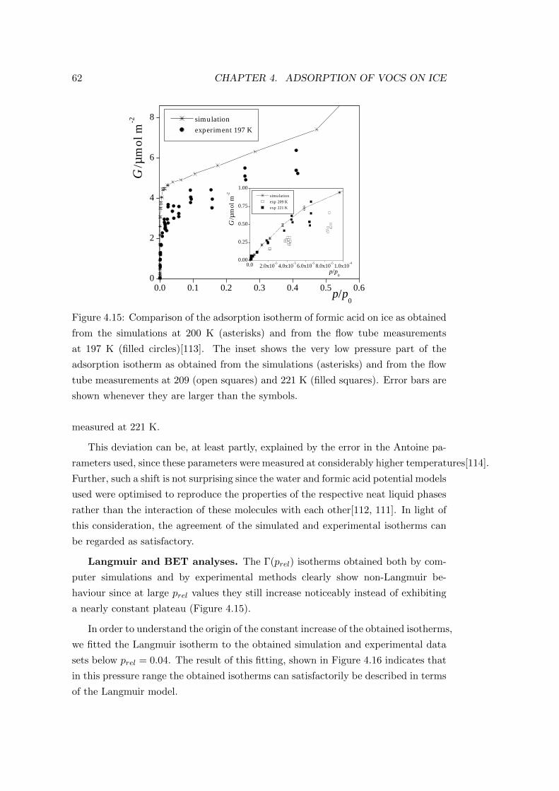
62 CHAPTER 4. ADSORPTION OF VOCS ON ICE
0.0 0.1 0.2 0.3 0.4 0.5 0.60
2
4
6
8
0.0 2.0x10⁻⁵ 4.0x10⁻⁵ 6.0x10⁻⁵ 8.0x10⁻⁵ 1.0x10-40.00
0.25
0.50
0.75
1.00
simulation experiment 197 K
Γ /µ
mol
m-2
p/p0
simulation exp 209 K exp 221 K
Γ /µ
mol
m-2
p/p0
Figure 4.15: Comparison of the adsorption isotherm of formic acid on ice as obtained
from the simulations at 200 K (asterisks) and from the flow tube measurements
at 197 K (filled circles)[113]. The inset shows the very low pressure part of the
adsorption isotherm as obtained from the simulations (asterisks) and from the flow
tube measurements at 209 (open squares) and 221 K (filled squares). Error bars are
shown whenever they are larger than the symbols.
measured at 221 K.
This deviation can be, at least partly, explained by the error in the Antoine pa-
rameters used, since these parameters were measured at considerably higher temperatures[114].
Further, such a shift is not surprising since the water and formic acid potential models
used were optimised to reproduce the properties of the respective neat liquid phases
rather than the interaction of these molecules with each other[112, 111]. In light of
this consideration, the agreement of the simulated and experimental isotherms can
be regarded as satisfactory.
Langmuir and BET analyses. The Γ(prel) isotherms obtained both by com-
puter simulations and by experimental methods clearly show non-Langmuir be-
haviour since at large prel values they still increase noticeably instead of exhibiting
a nearly constant plateau (Figure 4.15).
In order to understand the origin of the constant increase of the obtained isotherms,
we fitted the Langmuir isotherm to the obtained simulation and experimental data
sets below prel = 0.04. The result of this fitting, shown in Figure 4.16 indicates that
in this pressure range the obtained isotherms can satisfactorily be described in terms
of the Langmuir model.
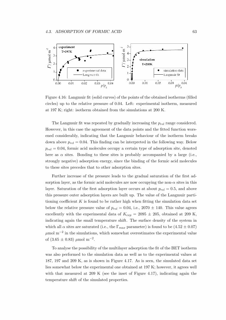
4.3. ADSORPTION OF FORMIC ACID 63
Figure 4.16: Langmuir fit (solid curves) of the points of the obtained isotherms (filled
circles) up to the relative pressure of 0.04. Left: experimental isotherm, measured
at 197 K; right: isotherm obtained from the simulations at 200 K.
The Langmuir fit was repeated by gradually increasing the prel range considered.
However, in this case the agreement of the data points and the fitted function wors-
ened considerably, indicating that the Langmuir behaviour of the isotherm breaks
down above prel = 0.04. This finding can be interpreted in the following way. Below
prel = 0.04, formic acid molecules occupy a certain type of adsorption site, denoted
here as α sites. Bonding to these sites is probably accompanied by a large (i.e.,
strongly negative) adsorption energy, since the binding of the formic acid molecules
to these sites precedes that to other adsorption sites.
Further increase of the pressure leads to the gradual saturation of the first ad-
sorption layer, as the formic acid molecules are now occupying the non-α sites in this
layer. Saturation of the first adsorption layer occurs at about prel = 0.5, and above
this pressure outer adsorption layers are built up. The value of the Langmuir parti-
tioning coefficient K is found to be rather high when fitting the simulation data set
below the relative pressure value of prel = 0.04, i.e., 2070 ± 140. This value agrees
excellently with the experimental data of Kexp = 2095 ± 205, obtained at 209 K,
indicating again the small temperature shift. The surface density of the system in
which all α sites are saturated (i.e., the Γmax parameter) is found to be (4.52 ± 0.07)
µmol m−2 in the simulations, which somewhat overestimates the experimental value
of (3.65 ± 0.83) µmol m−2.
To analyse the possibility of the multilayer adsorption the fit of the BET isotherm
was also performed to the simulation data as well as to the experimental values at
187, 197 and 209 K, as is shown in Figure 4.17. As is seen, the simulated data set
lies somewhat below the experimental one obtained at 197 K; however, it agrees well
with that measured at 209 K (see the inset of Figure 4.17), indicating again the
temperature shift of the simulated properties.
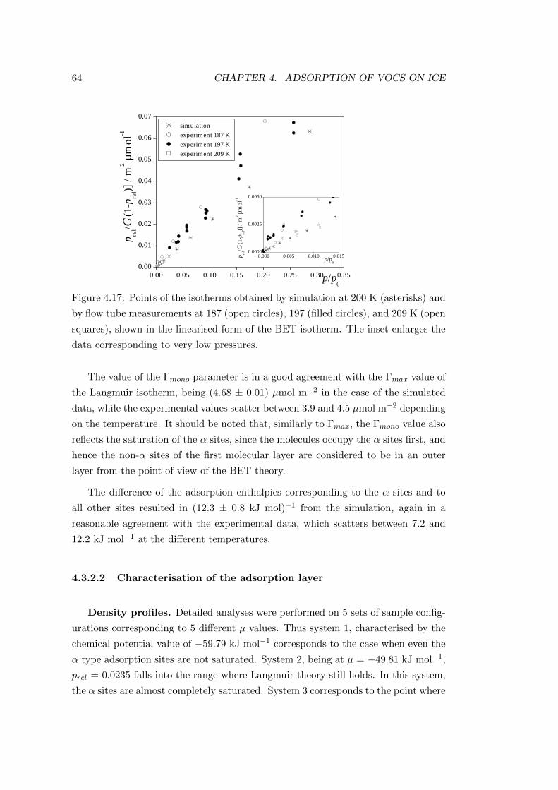
64 CHAPTER 4. ADSORPTION OF VOCS ON ICE
0.00 0.05 0.10 0.15 0.20 0.25 0.30 0.350.00
0.01
0.02
0.03
0.04
0.05
0.06
0.07
0.000 0.005 0.010 0.0150.0000
0.0025
0.0050
p rel/Γ
(1-p
rel)]
/ m
2 µm
ol-1
p/p0
simulation experiment 187 K experiment 197 K experiment 209 K
p/p0
p rel/Γ
(1-p
rel)]
/ m2 µ
mol
-1
Figure 4.17: Points of the isotherms obtained by simulation at 200 K (asterisks) and
by flow tube measurements at 187 (open circles), 197 (filled circles), and 209 K (open
squares), shown in the linearised form of the BET isotherm. The inset enlarges the
data corresponding to very low pressures.
The value of the Γmono parameter is in a good agreement with the Γmax value of
the Langmuir isotherm, being (4.68 ± 0.01) µmol m−2 in the case of the simulated
data, while the experimental values scatter between 3.9 and 4.5 µmol m−2 depending
on the temperature. It should be noted that, similarly to Γmax, the Γmono value also
reflects the saturation of the α sites, since the molecules occupy the α sites first, and
hence the non-α sites of the first molecular layer are considered to be in an outer
layer from the point of view of the BET theory.
The difference of the adsorption enthalpies corresponding to the α sites and to
all other sites resulted in (12.3 ± 0.8 kJ mol)−1 from the simulation, again in a
reasonable agreement with the experimental data, which scatters between 7.2 and
12.2 kJ mol−1 at the different temperatures.
4.3.2.2 Characterisation of the adsorption layer
Density profiles. Detailed analyses were performed on 5 sets of sample config-
urations corresponding to 5 different µ values. Thus system 1, characterised by the
chemical potential value of −59.79 kJ mol−1 corresponds to the case when even the
α type adsorption sites are not saturated. System 2, being at µ = −49.81 kJ mol−1,
prel = 0.0235 falls into the range where Langmuir theory still holds. In this system,
the α sites are almost completely saturated. System 3 corresponds to the point where
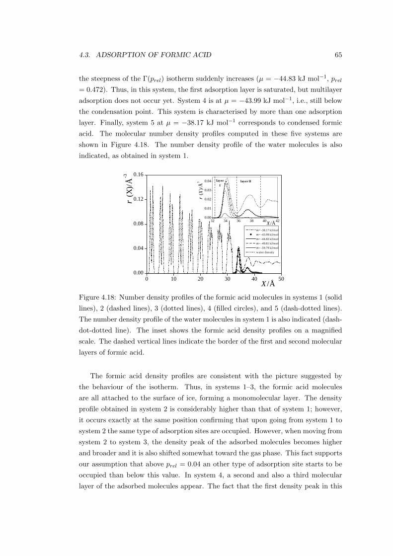
4.3. ADSORPTION OF FORMIC ACID 65
the steepness of the Γ(prel) isotherm suddenly increases (µ = −44.83 kJ mol−1, prel
= 0.472). Thus, in this system, the first adsorption layer is saturated, but multilayer
adsorption does not occur yet. System 4 is at µ = −43.99 kJ mol−1, i.e., still below
the condensation point. This system is characterised by more than one adsorption
layer. Finally, system 5 at µ = −38.17 kJ mol−1 corresponds to condensed formic
acid. The molecular number density profiles computed in these five systems are
shown in Figure 4.18. The number density profile of the water molecules is also
indicated, as obtained in system 1.
0 10 20 30 40 500.00
0.04
0.08
0.12
0.16
µ = -38.17 kJ/mol µ = -43.99 kJ/mol µ = -44.82 kJ/mol µ = -49.81 kJ/mol µ = -59.79 kJ/mol water density
ρ
(X)/Å
-3
X/Å
32 34 36 38 40 420.00
0.01
0.02
0.03
0.04 layerI
layer II
X/Å
ρ (X
)/Å3
Figure 4.18: Number density profiles of the formic acid molecules in systems 1 (solid
lines), 2 (dashed lines), 3 (dotted lines), 4 (filled circles), and 5 (dash-dotted lines).
The number density profile of the water molecules in system 1 is also indicated (dash-
dot-dotted line). The inset shows the formic acid density profiles on a magnified
scale. The dashed vertical lines indicate the border of the first and second molecular
layers of formic acid.
The formic acid density profiles are consistent with the picture suggested by
the behaviour of the isotherm. Thus, in systems 1–3, the formic acid molecules
are all attached to the surface of ice, forming a monomolecular layer. The density
profile obtained in system 2 is considerably higher than that of system 1; however,
it occurs exactly at the same position confirming that upon going from system 1 to
system 2 the same type of adsorption sites are occupied. However, when moving from
system 2 to system 3, the density peak of the adsorbed molecules becomes higher
and broader and it is also shifted somewhat toward the gas phase. This fact supports
our assumption that above prel = 0.04 an other type of adsorption site starts to be
occupied than below this value. In system 4, a second and also a third molecular
layer of the adsorbed molecules appear. The fact that the first density peak in this
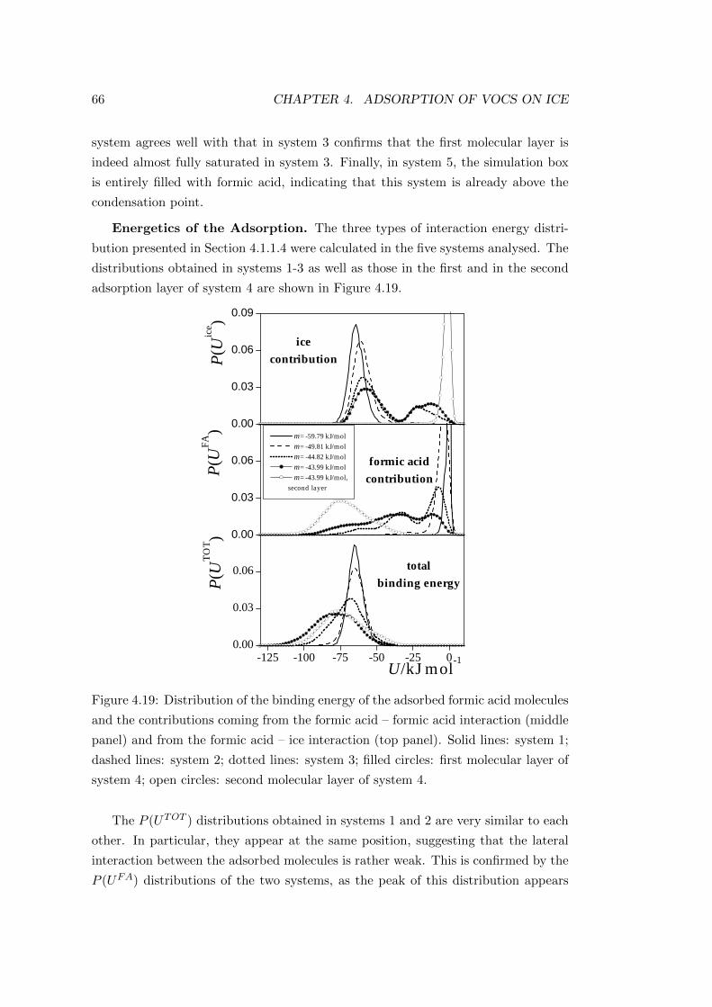
66 CHAPTER 4. ADSORPTION OF VOCS ON ICE
system agrees well with that in system 3 confirms that the first molecular layer is
indeed almost fully saturated in system 3. Finally, in system 5, the simulation box
is entirely filled with formic acid, indicating that this system is already above the
condensation point.
Energetics of the Adsorption. The three types of interaction energy distri-
bution presented in Section 4.1.1.4 were calculated in the five systems analysed. The
distributions obtained in systems 1-3 as well as those in the first and in the second
adsorption layer of system 4 are shown in Figure 4.19.
0.00
0.03
0.06
0.09
0.00
0.03
0.06
-125 -100 -75 -50 -25 00.00
0.03
0.06
icecontribution
totalbinding energy
formic acidcontribution
P(U
ice )
µ = -59.79 kJ/mol µ = -49.81 kJ/mol µ = -44.82 kJ/mol µ = -43.99 kJ/mol µ = -43.99 kJ/mol,
second layer
P(U
FA)
P(U
TOT )
U/kJ mol-1
Figure 4.19: Distribution of the binding energy of the adsorbed formic acid molecules
and the contributions coming from the formic acid – formic acid interaction (middle
panel) and from the formic acid – ice interaction (top panel). Solid lines: system 1;
dashed lines: system 2; dotted lines: system 3; filled circles: first molecular layer of
system 4; open circles: second molecular layer of system 4.
The P (UTOT ) distributions obtained in systems 1 and 2 are very similar to each
other. In particular, they appear at the same position, suggesting that the lateral
interaction between the adsorbed molecules is rather weak. This is confirmed by the
P (UFA) distributions of the two systems, as the peak of this distribution appears
4.3. ADSORPTION OF FORMIC ACID 67
very close to zero in both cases. Upon further saturation the peak of the total
binding energy distribution gradually shifts to lower energies due to the increasing
lateral interactions. The P (UTOT ) distributions obtained in the first and second
layers of system 4 are rather close to each other; the mean binding energy value is
−78.4 kJ mol−1 in the first and −72.3 kJ mol−1 in the second layer.
The distributions of the P (U ice) and P (UFA) contributions to the total bind-
ing energy show a more detailed picture. Thus, in systems 1 and 2, the P (U ice)
distribution is unimodal, having its peak at very low energies, between −61 and
−64 kJ mol−1, indicating that formic acid molecules form two exceptionally strong
hydrogen bonds with the ice surface at the α positions. These values are also in a
reasonable agreement with the experimental value of the heat of adsorption of (−54
± 8) kJ mol−1, determined from the temperature dependence of the isotherm in very
low pressure range[113].
Upon increasing the surface coverage, another peak of P (U ice) appears at con-
siderably higher energies, i.e., around −20 kJ mol−1. The bimodal shape of P (U ice)
in systems 3 and 4 is in accordance with our former conclusion that the saturation of
the α sites is followed by further saturation of the first molecular layer by occupying
other (non-α) sites. The position of this second peak of P (U ice) indicates that at
these sites, the adsorbed formic acid molecules cannot form more than one hydrogen
bond, and this hydrogen bond is weaker than those formed at α positions.
However, this weak binding of the adsorbed molecules at non-α positions is ac-
companied by rather strong lateral interactions between these molecules. Thus, the
P (UFA) distribution in system 3 as well as that in the first layer of system 4 is
trimodal. The peak closest to zero can be associated with the molecules being at α
positions since these molecules do not have strong (hydrogen-bonding) interactions
with their neighbours. The second peak, located at about −33 kJ mol−1, is given by
the molecules that form only one strong (O-H· · · O type) hydrogen bond with other
formic acids. The unusual broadness of this peak suggests that some of these mole-
cules probably also form a weak C-H· · ·O type hydrogen bond with another formic
acid molecule. Finally, the peak located at the lowest energies is clearly given by the
molecules that form two strong, O-H· · ·O type hydrogen bond with their neighbours.
It is also seen that in the second layer of system 4, the P (UFA) distribution is
again unimodal, having its peak at about −75 kJ mol−1, indicating that in the second
layer, the majority of the formic acid molecules maintain two strong O-H· · ·O type
hydrogen bonds with their neighbours, probably by forming pairs of cyclic hydrogen-
bonded dimers. This finding is also in accordance both with the former computer
simulation result of Picaud and co-workers[80] and with the experimental finding of
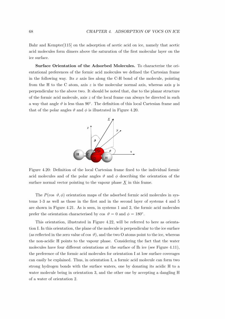
68 CHAPTER 4. ADSORPTION OF VOCS ON ICE
Bahr and Kempter[115] on the adsorption of acetic acid on ice, namely that acetic
acid molecules form dimers above the saturation of the first molecular layer on the
ice surface.
Surface Orientation of the Adsorbed Molecules. To characterise the ori-
entational preferences of the formic acid molecules we defined the Cartesian frame
in the following way. Its x axis lies along the C-H bond of the molecule, pointing
from the H to the C atom, axis z is the molecular normal axis, whereas axis y is
perpendicular to the above two. It should be noted that, due to the planar structure
of the formic acid molecule, axis z of the local frame can always be directed in such
a way that angle ϑ is less than 90. The definition of this local Cartesian frame and
that of the polar angles ϑ and φ is illustrated in Figure 4.20.
Figure 4.20: Definition of the local Cartesian frame fixed to the individual formic
acid molecules and of the polar angles ϑ and φ describing the orientation of the
surface normal vector pointing to the vapour phase X in this frame.
The P (cos ϑ, φ) orientation maps of the adsorbed formic acid molecules in sys-
tems 1-3 as well as those in the first and in the second layer of systems 4 and 5
are shown in Figure 4.21. As is seen, in systems 1 and 2, the formic acid molecules
prefer the orientation characterised by cos ϑ = 0 and φ = 180.
This orientation, illustrated in Figure 4.22, will be referred to here as orienta-
tion I. In this orientation, the plane of the molecule is perpendicular to the ice surface
(as reflected in the zero value of cos ϑ), and the two O atoms point to the ice, whereas
the non-acidic H points to the vapour phase. Considering the fact that the water
molecules have four different orientations at the surface of Ih ice (see Figure 4.11),
the preference of the formic acid molecules for orientation I at low surface coverages
can easily be explained. Thus, in orientation I, a formic acid molecule can form two
strong hydrogen bonds with the surface waters, one by donating its acidic H to a
water molecule being in orientation 3, and the other one by accepting a dangling H
of a water of orientation 2.
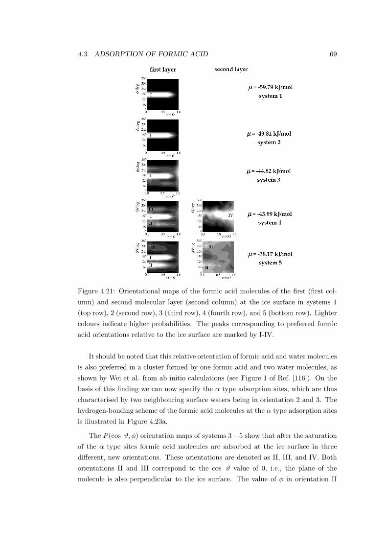
4.3. ADSORPTION OF FORMIC ACID 69
Figure 4.21: Orientational maps of the formic acid molecules of the first (first col-
umn) and second molecular layer (second column) at the ice surface in systems 1
(top row), 2 (second row), 3 (third row), 4 (fourth row), and 5 (bottom row). Lighter
colours indicate higher probabilities. The peaks corresponding to preferred formic
acid orientations relative to the ice surface are marked by I-IV.
It should be noted that this relative orientation of formic acid and water molecules
is also preferred in a cluster formed by one formic acid and two water molecules, as
shown by Wei et al. from ab initio calculations (see Figure 1 of Ref. [116]). On the
basis of this finding we can now specify the α type adsorption sites, which are thus
characterised by two neighbouring surface waters being in orientation 2 and 3. The
hydrogen-bonding scheme of the formic acid molecules at the α type adsorption sites
is illustrated in Figure 4.23a.
The P (cos ϑ, φ) orientation maps of systems 3 – 5 show that after the saturation
of the α type sites formic acid molecules are adsorbed at the ice surface in three
different, new orientations. These orientations are denoted as II, III, and IV. Both
orientations II and III correspond to the cos ϑ value of 0, i.e., the plane of the
molecule is also perpendicular to the ice surface. The value of φ in orientation II
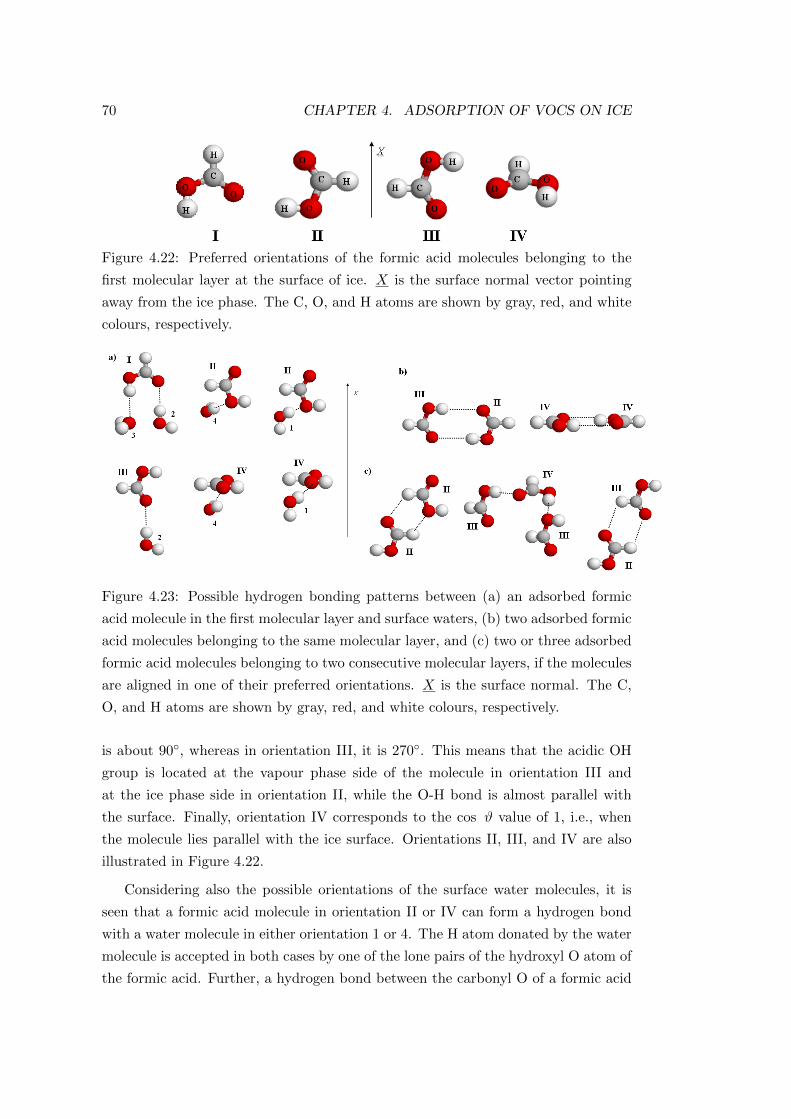
70 CHAPTER 4. ADSORPTION OF VOCS ON ICE
Figure 4.22: Preferred orientations of the formic acid molecules belonging to the
first molecular layer at the surface of ice. X is the surface normal vector pointing
away from the ice phase. The C, O, and H atoms are shown by gray, red, and white
colours, respectively.
Figure 4.23: Possible hydrogen bonding patterns between (a) an adsorbed formic
acid molecule in the first molecular layer and surface waters, (b) two adsorbed formic
acid molecules belonging to the same molecular layer, and (c) two or three adsorbed
formic acid molecules belonging to two consecutive molecular layers, if the molecules
are aligned in one of their preferred orientations. X is the surface normal. The C,
O, and H atoms are shown by gray, red, and white colours, respectively.
is about 90, whereas in orientation III, it is 270. This means that the acidic OH
group is located at the vapour phase side of the molecule in orientation III and
at the ice phase side in orientation II, while the O-H bond is almost parallel with
the surface. Finally, orientation IV corresponds to the cos ϑ value of 1, i.e., when
the molecule lies parallel with the ice surface. Orientations II, III, and IV are also
illustrated in Figure 4.22.
Considering also the possible orientations of the surface water molecules, it is
seen that a formic acid molecule in orientation II or IV can form a hydrogen bond
with a water molecule in either orientation 1 or 4. The H atom donated by the water
molecule is accepted in both cases by one of the lone pairs of the hydroxyl O atom of
the formic acid. Further, a hydrogen bond between the carbonyl O of a formic acid
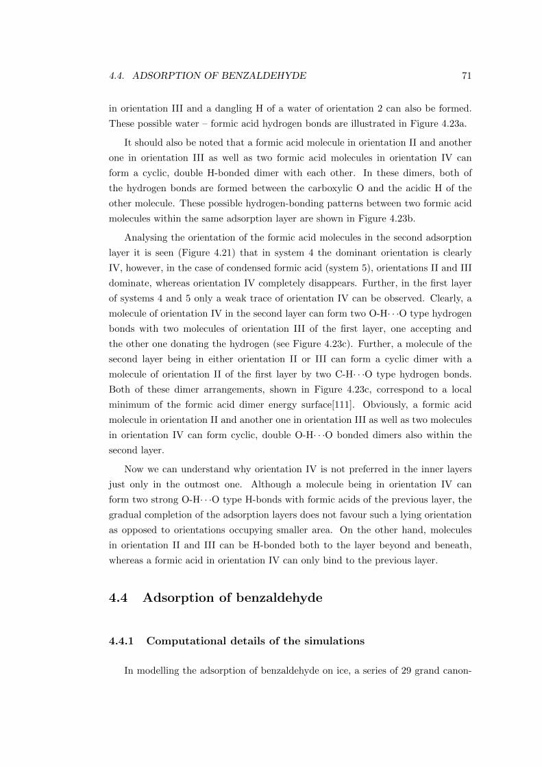
4.4. ADSORPTION OF BENZALDEHYDE 71
in orientation III and a dangling H of a water of orientation 2 can also be formed.
These possible water – formic acid hydrogen bonds are illustrated in Figure 4.23a.
It should also be noted that a formic acid molecule in orientation II and another
one in orientation III as well as two formic acid molecules in orientation IV can
form a cyclic, double H-bonded dimer with each other. In these dimers, both of
the hydrogen bonds are formed between the carboxylic O and the acidic H of the
other molecule. These possible hydrogen-bonding patterns between two formic acid
molecules within the same adsorption layer are shown in Figure 4.23b.
Analysing the orientation of the formic acid molecules in the second adsorption
layer it is seen (Figure 4.21) that in system 4 the dominant orientation is clearly
IV, however, in the case of condensed formic acid (system 5), orientations II and III
dominate, whereas orientation IV completely disappears. Further, in the first layer
of systems 4 and 5 only a weak trace of orientation IV can be observed. Clearly, a
molecule of orientation IV in the second layer can form two O-H· · ·O type hydrogen
bonds with two molecules of orientation III of the first layer, one accepting and
the other one donating the hydrogen (see Figure 4.23c). Further, a molecule of the
second layer being in either orientation II or III can form a cyclic dimer with a
molecule of orientation II of the first layer by two C-H· · ·O type hydrogen bonds.
Both of these dimer arrangements, shown in Figure 4.23c, correspond to a local
minimum of the formic acid dimer energy surface[111]. Obviously, a formic acid
molecule in orientation II and another one in orientation III as well as two molecules
in orientation IV can form cyclic, double O-H· · ·O bonded dimers also within the
second layer.
Now we can understand why orientation IV is not preferred in the inner layers
just only in the outmost one. Although a molecule being in orientation IV can
form two strong O-H· · ·O type H-bonds with formic acids of the previous layer, the
gradual completion of the adsorption layers does not favour such a lying orientation
as opposed to orientations occupying smaller area. On the other hand, molecules
in orientation II and III can be H-bonded both to the layer beyond and beneath,
whereas a formic acid in orientation IV can only bind to the previous layer.
4.4 Adsorption of benzaldehyde
4.4.1 Computational details of the simulations
In modelling the adsorption of benzaldehyde on ice, a series of 29 grand canon-
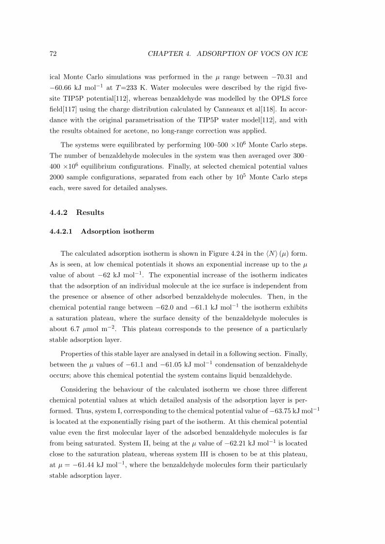
72 CHAPTER 4. ADSORPTION OF VOCS ON ICE
ical Monte Carlo simulations was performed in the µ range between −70.31 and
−60.66 kJ mol−1 at T=233 K. Water molecules were described by the rigid five-
site TIP5P potential[112], whereas benzaldehyde was modelled by the OPLS force
field[117] using the charge distribution calculated by Canneaux et al[118]. In accor-
dance with the original parametrisation of the TIP5P water model[112], and with
the results obtained for acetone, no long-range correction was applied.
The systems were equilibrated by performing 100–500 ×106 Monte Carlo steps.
The number of benzaldehyde molecules in the system was then averaged over 300–
400 ×106 equilibrium configurations. Finally, at selected chemical potential values
2000 sample configurations, separated from each other by 105 Monte Carlo steps
each, were saved for detailed analyses.
4.4.2 Results
4.4.2.1 Adsorption isotherm
The calculated adsorption isotherm is shown in Figure 4.24 in the 〈N〉 (µ) form.
As is seen, at low chemical potentials it shows an exponential increase up to the µ
value of about −62 kJ mol−1. The exponential increase of the isotherm indicates
that the adsorption of an individual molecule at the ice surface is independent from
the presence or absence of other adsorbed benzaldehyde molecules. Then, in the
chemical potential range between −62.0 and −61.1 kJ mol−1 the isotherm exhibits
a saturation plateau, where the surface density of the benzaldehyde molecules is
about 6.7 µmol m−2. This plateau corresponds to the presence of a particularly
stable adsorption layer.
Properties of this stable layer are analysed in detail in a following section. Finally,
between the µ values of −61.1 and −61.05 kJ mol−1 condensation of benzaldehyde
occurs; above this chemical potential the system contains liquid benzaldehyde.
Considering the behaviour of the calculated isotherm we chose three different
chemical potential values at which detailed analysis of the adsorption layer is per-
formed. Thus, system I, corresponding to the chemical potential value of−63.75 kJ mol−1
is located at the exponentially rising part of the isotherm. At this chemical potential
value even the first molecular layer of the adsorbed benzaldehyde molecules is far
from being saturated. System II, being at the µ value of −62.21 kJ mol−1 is located
close to the saturation plateau, whereas system III is chosen to be at this plateau,
at µ = −61.44 kJ mol−1, where the benzaldehyde molecules form their particularly
stable adsorption layer.
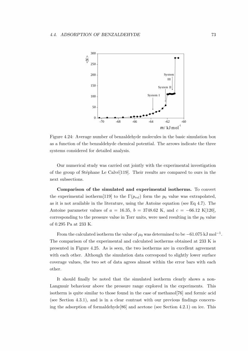
4.4. ADSORPTION OF BENZALDEHYDE 73
-70 -68 -66 -64 -62 -600
50
100
150
200
250
300
SystemIII
System II
System I
<N>
µ / kJ mol-1
Figure 4.24: Average number of benzaldehyde molecules in the basic simulation box
as a function of the benzaldehyde chemical potential. The arrows indicate the three
systems considered for detailed analysis.
Our numerical study was carried out jointly with the experimental investigation
of the group of Stephane Le Calve[119]. Their results are compared to ours in the
next subsections.
Comparison of the simulated and experimental isotherms. To convert
the experimental isotherm[119] to the Γ(prel) form the p0 value was extrapolated,
as it is not available in the literature, using the Antoine equation (see Eq 4.7). The
Antoine parameter values of a = 16.35, b = 3748.62 K, and c = −66.12 K[120],
corresponding to the pressure value in Torr units, were used resulting in the p0 value
of 0.295 Pa at 233 K.
From the calculated isotherm the value of µ0 was determined to be−61.075 kJ mol−1.
The comparison of the experimental and calculated isotherms obtained at 233 K is
presented in Figure 4.25. As is seen, the two isotherms are in excellent agreement
with each other. Although the simulation data correspond to slightly lower surface
coverage values, the two set of data agrees almost within the error bars with each
other.
It should finally be noted that the simulated isotherm clearly shows a non-
Langmuir behaviour above the pressure range explored in the experiments. This
isotherm is quite similar to those found in the case of methanol[76] and formic acid
(see Section 4.3.1), and is in a clear contrast with our previous findings concern-
ing the adsorption of formaldehyde[86] and acetone (see Section 4.2.1) on ice. This
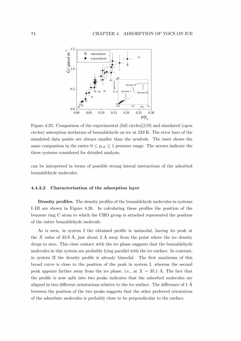
74 CHAPTER 4. ADSORPTION OF VOCS ON ICE
0.00 0.05 0.10 0.15 0.20 0.25 0.300.0
0.5
1.0
1.5
0.0 0.5 1.00
4
8
simulation experiment
System II
System I System III
Γ / µ
mol
m-2
p/p0
Γ / µ
mol
m-2
p/p0
Figure 4.25: Comparison of the experimental (full circles)[119] and simulated (open
circles) adsorption isotherms of benzaldehyde on ice at 233 K. The error bars of the
simulated data points are always smaller than the symbols. The inset shows the
same comparison in the entire 0 ≤ prel ≤ 1 pressure range. The arrows indicate the
three systems considered for detailed analysis.
can be interpreted in terms of possible strong lateral interactions of the adsorbed
benzaldehyde molecules.
4.4.2.2 Characterisation of the adsorption layer
Density profiles. The density profiles of the benzaldehyde molecules in systems
I–III are shown in Figure 4.26. In calculating these profiles the position of the
benzene ring C atom to which the CHO group is attached represented the position
of the entire benzaldehyde molecule.
As is seen, in system I the obtained profile is unimodal, having its peak at
the X value of 33.9 A, just about 2 A away from the point where the ice density
drops to zero. This close contact with the ice phase suggests that the benzaldehyde
molecules in this system are probably lying parallel with the ice surface. In contrast,
in system II the density profile is already bimodal. The first maximum of this
broad curve is close to the position of the peak in system I, whereas the second
peak appears farther away from the ice phase, i.e., at X = 35.1 A. The fact that
the profile is now split into two peaks indicates that the adsorbed molecules are
aligned in two different orientations relative to the ice surface. The difference of 1 A
between the position of the two peaks suggests that the other preferred orientation
of the adsorbate molecules is probably close to be perpendicular to the surface.
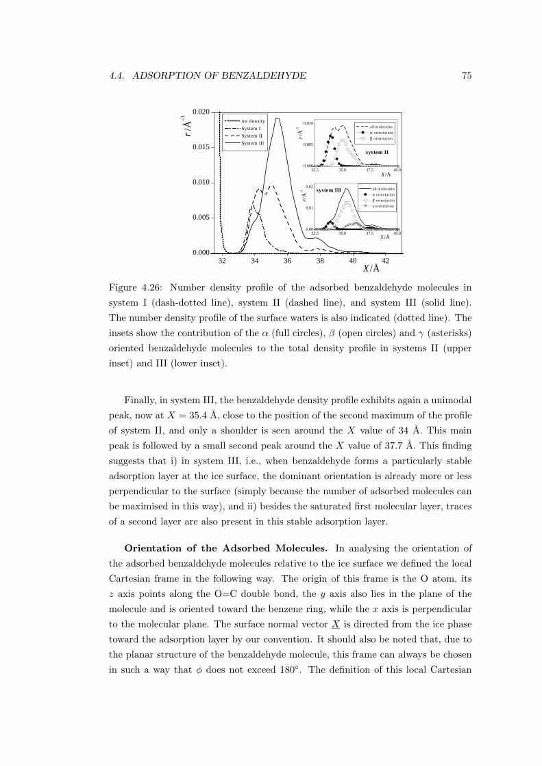
4.4. ADSORPTION OF BENZALDEHYDE 75
32 34 36 38 40 420.000
0.005
0.010
0.015
0.020
32.5 35.0 37.5 40.00.000
0.005
0.010
32.5 35.0 37.5 40.00.00
0.01
0.02
ice density System I System II System III
ρ/Å
-3
X/Å
system II
all molecules α orientation β orientation
ρ/Å
-3
X/Å
system III all molecules α orientation β orientation γ orientation
ρ/Å
-3
X/Å
Figure 4.26: Number density profile of the adsorbed benzaldehyde molecules in
system I (dash-dotted line), system II (dashed line), and system III (solid line).
The number density profile of the surface waters is also indicated (dotted line). The
insets show the contribution of the α (full circles), β (open circles) and γ (asterisks)
oriented benzaldehyde molecules to the total density profile in systems II (upper
inset) and III (lower inset).
Finally, in system III, the benzaldehyde density profile exhibits again a unimodal
peak, now at X = 35.4 A, close to the position of the second maximum of the profile
of system II, and only a shoulder is seen around the X value of 34 A. This main
peak is followed by a small second peak around the X value of 37.7 A. This finding
suggests that i) in system III, i.e., when benzaldehyde forms a particularly stable
adsorption layer at the ice surface, the dominant orientation is already more or less
perpendicular to the surface (simply because the number of adsorbed molecules can
be maximised in this way), and ii) besides the saturated first molecular layer, traces
of a second layer are also present in this stable adsorption layer.
Orientation of the Adsorbed Molecules. In analysing the orientation of
the adsorbed benzaldehyde molecules relative to the ice surface we defined the local
Cartesian frame in the following way. The origin of this frame is the O atom, its
z axis points along the O=C double bond, the y axis also lies in the plane of the
molecule and is oriented toward the benzene ring, while the x axis is perpendicular
to the molecular plane. The surface normal vector X is directed from the ice phase
toward the adsorption layer by our convention. It should also be noted that, due to
the planar structure of the benzaldehyde molecule, this frame can always be chosen
in such a way that φ does not exceed 180. The definition of this local Cartesian
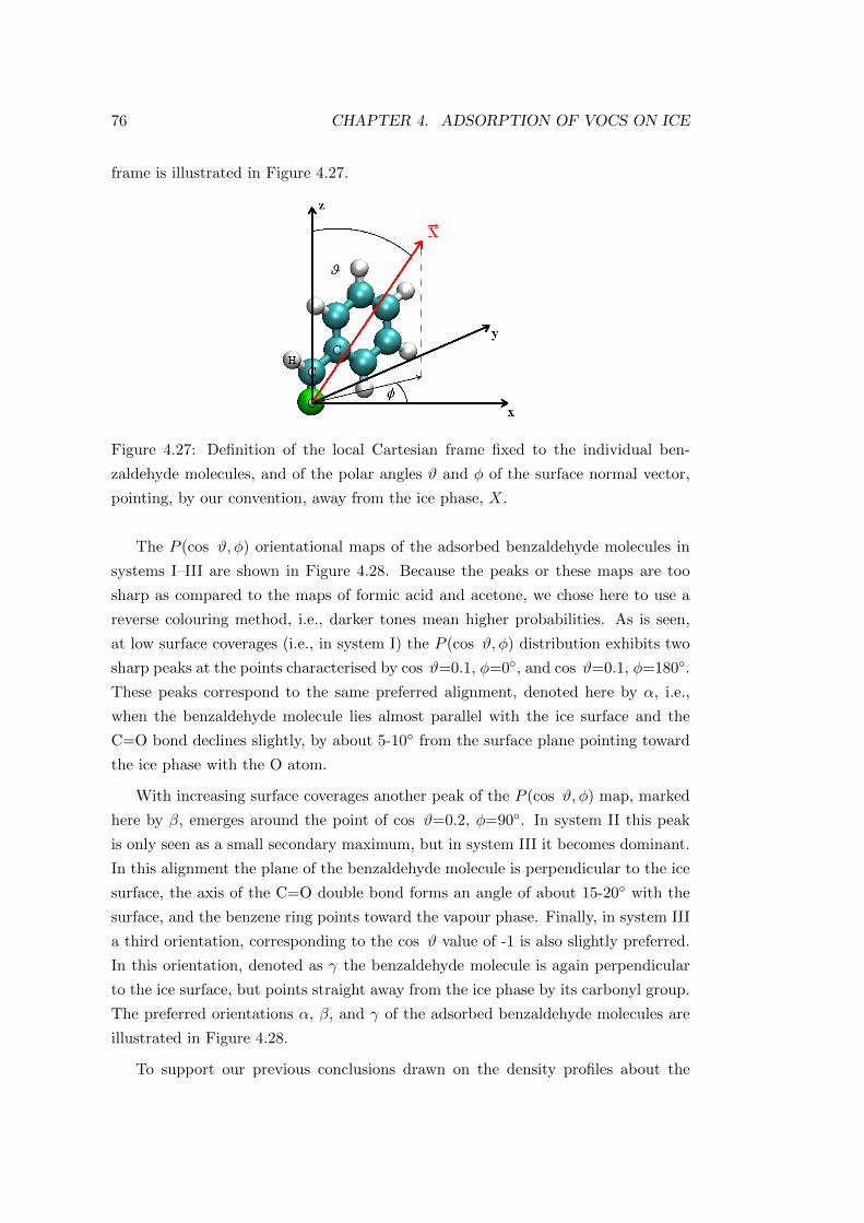
76 CHAPTER 4. ADSORPTION OF VOCS ON ICE
frame is illustrated in Figure 4.27.
Figure 4.27: Definition of the local Cartesian frame fixed to the individual ben-
zaldehyde molecules, and of the polar angles ϑ and φ of the surface normal vector,
pointing, by our convention, away from the ice phase, X.
The P (cos ϑ, φ) orientational maps of the adsorbed benzaldehyde molecules in
systems I–III are shown in Figure 4.28. Because the peaks or these maps are too
sharp as compared to the maps of formic acid and acetone, we chose here to use a
reverse colouring method, i.e., darker tones mean higher probabilities. As is seen,
at low surface coverages (i.e., in system I) the P (cos ϑ, φ) distribution exhibits two
sharp peaks at the points characterised by cos ϑ=0.1, φ=0, and cos ϑ=0.1, φ=180.
These peaks correspond to the same preferred alignment, denoted here by α, i.e.,
when the benzaldehyde molecule lies almost parallel with the ice surface and the
C=O bond declines slightly, by about 5-10 from the surface plane pointing toward
the ice phase with the O atom.
With increasing surface coverages another peak of the P (cos ϑ, φ) map, marked
here by β, emerges around the point of cos ϑ=0.2, φ=90. In system II this peak
is only seen as a small secondary maximum, but in system III it becomes dominant.
In this alignment the plane of the benzaldehyde molecule is perpendicular to the ice
surface, the axis of the C=O double bond forms an angle of about 15-20 with the
surface, and the benzene ring points toward the vapour phase. Finally, in system III
a third orientation, corresponding to the cos ϑ value of -1 is also slightly preferred.
In this orientation, denoted as γ the benzaldehyde molecule is again perpendicular
to the ice surface, but points straight away from the ice phase by its carbonyl group.
The preferred orientations α, β, and γ of the adsorbed benzaldehyde molecules are
illustrated in Figure 4.28.
To support our previous conclusions drawn on the density profiles about the
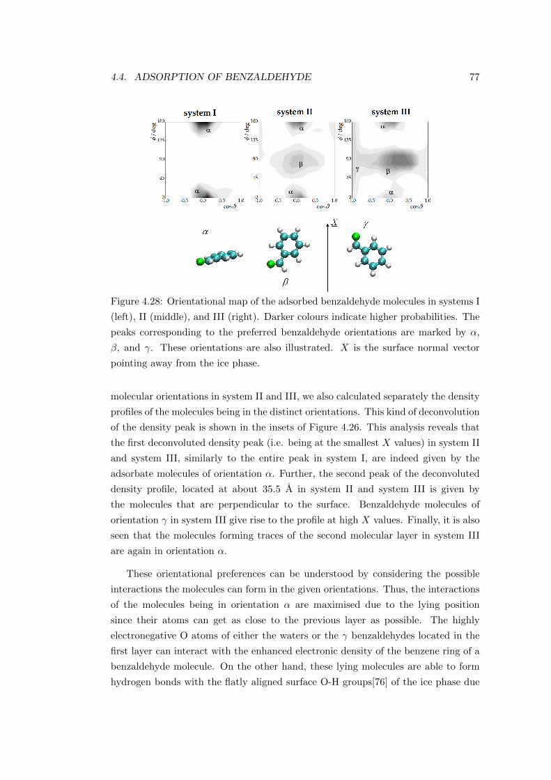
4.4. ADSORPTION OF BENZALDEHYDE 77
Figure 4.28: Orientational map of the adsorbed benzaldehyde molecules in systems I
(left), II (middle), and III (right). Darker colours indicate higher probabilities. The
peaks corresponding to the preferred benzaldehyde orientations are marked by α,
β, and γ. These orientations are also illustrated. X is the surface normal vector
pointing away from the ice phase.
molecular orientations in system II and III, we also calculated separately the density
profiles of the molecules being in the distinct orientations. This kind of deconvolution
of the density peak is shown in the insets of Figure 4.26. This analysis reveals that
the first deconvoluted density peak (i.e. being at the smallest X values) in system II
and system III, similarly to the entire peak in system I, are indeed given by the
adsorbate molecules of orientation α. Further, the second peak of the deconvoluted
density profile, located at about 35.5 A in system II and system III is given by
the molecules that are perpendicular to the surface. Benzaldehyde molecules of
orientation γ in system III give rise to the profile at high X values. Finally, it is also
seen that the molecules forming traces of the second molecular layer in system III
are again in orientation α.
These orientational preferences can be understood by considering the possible
interactions the molecules can form in the given orientations. Thus, the interactions
of the molecules being in orientation α are maximised due to the lying position
since their atoms can get as close to the previous layer as possible. The highly
electronegative O atoms of either the waters or the γ benzaldehydes located in the
first layer can interact with the enhanced electronic density of the benzene ring of a
benzaldehyde molecule. On the other hand, these lying molecules are able to form
hydrogen bonds with the flatly aligned surface O-H groups[76] of the ice phase due
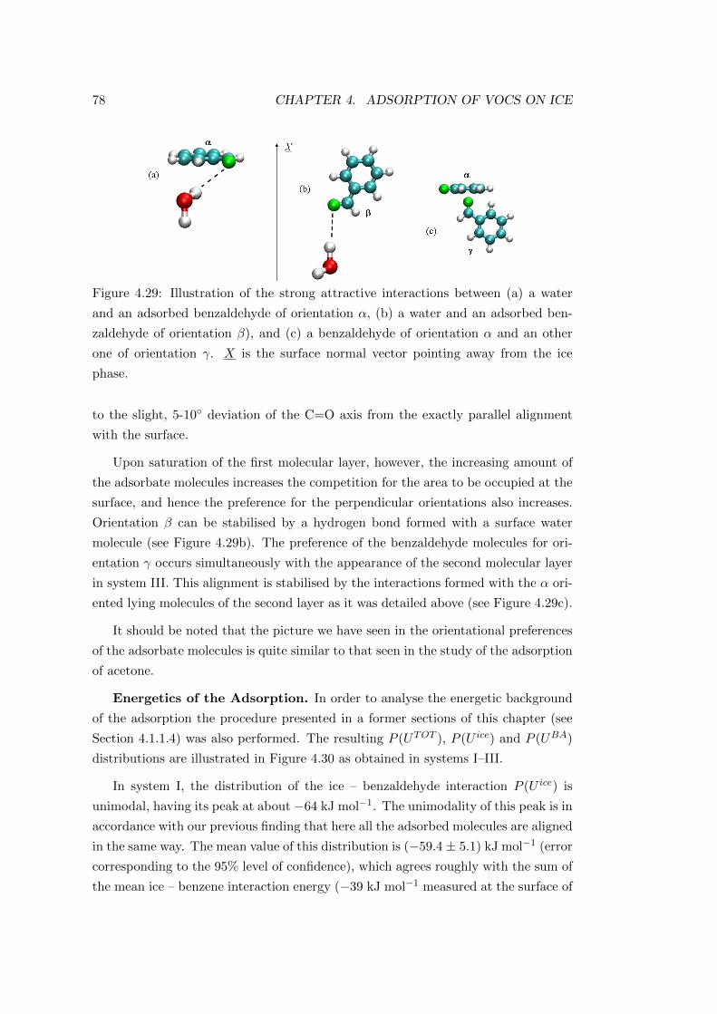
78 CHAPTER 4. ADSORPTION OF VOCS ON ICE
Figure 4.29: Illustration of the strong attractive interactions between (a) a water
and an adsorbed benzaldehyde of orientation α, (b) a water and an adsorbed ben-
zaldehyde of orientation β), and (c) a benzaldehyde of orientation α and an other
one of orientation γ. X is the surface normal vector pointing away from the ice
phase.
to the slight, 5-10 deviation of the C=O axis from the exactly parallel alignment
with the surface.
Upon saturation of the first molecular layer, however, the increasing amount of
the adsorbate molecules increases the competition for the area to be occupied at the
surface, and hence the preference for the perpendicular orientations also increases.
Orientation β can be stabilised by a hydrogen bond formed with a surface water
molecule (see Figure 4.29b). The preference of the benzaldehyde molecules for ori-
entation γ occurs simultaneously with the appearance of the second molecular layer
in system III. This alignment is stabilised by the interactions formed with the α ori-
ented lying molecules of the second layer as it was detailed above (see Figure 4.29c).
It should be noted that the picture we have seen in the orientational preferences
of the adsorbate molecules is quite similar to that seen in the study of the adsorption
of acetone.
Energetics of the Adsorption. In order to analyse the energetic background
of the adsorption the procedure presented in a former sections of this chapter (see
Section 4.1.1.4) was also performed. The resulting P (UTOT ), P (U ice) and P (UBA)
distributions are illustrated in Figure 4.30 as obtained in systems I–III.
In system I, the distribution of the ice – benzaldehyde interaction P (U ice) is
unimodal, having its peak at about −64 kJ mol−1. The unimodality of this peak is in
accordance with our previous finding that here all the adsorbed molecules are aligned
in the same way. The mean value of this distribution is (−59.4 ± 5.1) kJ mol−1 (error
corresponding to the 95% level of confidence), which agrees roughly with the sum of
the mean ice – benzene interaction energy (−39 kJ mol−1 measured at the surface of
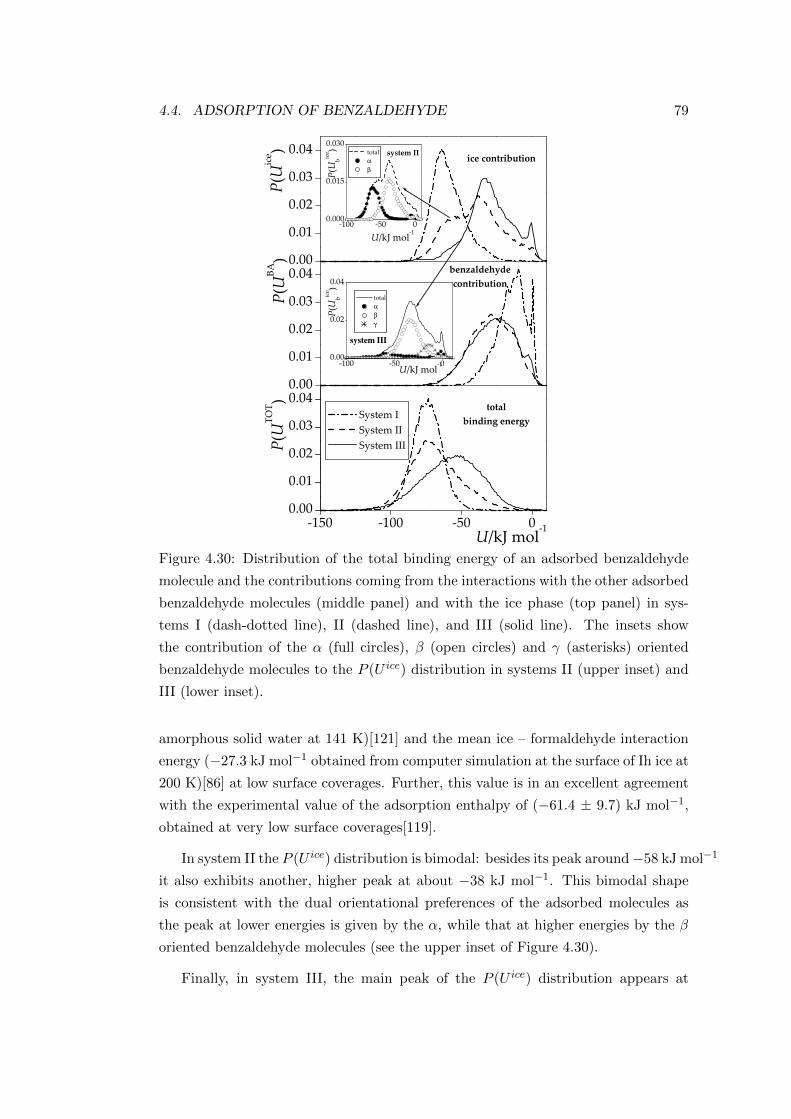
4.4. ADSORPTION OF BENZALDEHYDE 79
αβ
system III
αβγ
Figure 4.30: Distribution of the total binding energy of an adsorbed benzaldehyde
molecule and the contributions coming from the interactions with the other adsorbed
benzaldehyde molecules (middle panel) and with the ice phase (top panel) in sys-
tems I (dash-dotted line), II (dashed line), and III (solid line). The insets show
the contribution of the α (full circles), β (open circles) and γ (asterisks) oriented
benzaldehyde molecules to the P (U ice) distribution in systems II (upper inset) and
III (lower inset).
amorphous solid water at 141 K)[121] and the mean ice – formaldehyde interaction
energy (−27.3 kJ mol−1 obtained from computer simulation at the surface of Ih ice at
200 K)[86] at low surface coverages. Further, this value is in an excellent agreement
with the experimental value of the adsorption enthalpy of (−61.4 ± 9.7) kJ mol−1,
obtained at very low surface coverages[119].
In system II the P (U ice) distribution is bimodal: besides its peak around−58 kJ mol−1
it also exhibits another, higher peak at about −38 kJ mol−1. This bimodal shape
is consistent with the dual orientational preferences of the adsorbed molecules as
the peak at lower energies is given by the α, while that at higher energies by the β
oriented benzaldehyde molecules (see the upper inset of Figure 4.30).
Finally, in system III, the main peak of the P (U ice) distribution appears at
80 CHAPTER 4. ADSORPTION OF VOCS ON ICE
about −34 kJ mol−1, and it has also two shoulders located at −58 kJ mol−1 and
−14 kJ mol−1. This distribution has also a second peak of smaller intensity close
to zero. As is expected, the shoulder at low energies is given by the few α oriented
molecules, while the main peak is related to the β oriented molecules. The high
energy shoulder can be attributed to the molecules of orientation γ, whereas the
peak around zero energies is given by the molecules of the second molecular layer as
they are already far from the surface (see the lower inset of Figure 4.30).
The P (UBA) distribution has a peak at zero and another one around−10 kJ mol−1
in system I. The zero energy peak is clearly coming from the isolated benzaldehyde
molecules. The presence of the other peak in the system of low surface coverage
indicates the tendency of the adsorbed benzaldehyde molecules for forming lateral
self-aggregates rather than being always isolated from each other. At higher surface
coverages, however, the P (UBA) distribution becomes unimodal, having its peak
around −28 kJ mol−1. This energy might be related to the π–π and dipole–dipole
type interaction of the neighbouring adsorbate molecules.
The distribution of the entire binding energy P (UTOT ) exhibits a single peak
around −75 kJ mol−1 both in system I and system II. The total energy of the
adsorption of a benzaldehyde molecule in these systems is rather low, and is also
comparable with multiple hydrogen bond forming adsorbates such as methanol[76]
or formic acid (see Section 4.3.1). The lack of the possibility of multiple hydrogen
bond formation is compensated here by either the strong interaction formed between
the benzene ring and a strongly electronegative O atom or the π–π and dipole–
dipole type interactions between two perpendicularly oriented adsorbate molecules.
Further increase of the surface coverage leads to somewhat weaker average attraction
experienced by the individual molecules, as is reflected in the fact that the peak of the
P (UTOT ) distribution appears around −50 kJ mol−1 in system III. This weakening
of the average binding energy is, however, overcompensated by the large increase
of the number of adsorbed molecules, making thus the saturated adsorption layer
considerably stable.
4.5 Conclusions
In this chapter we have presented a numerical procedure enabling us to thor-
oughly investigate adsorption processes in computer simulations based on the GCMC
method, as it has been demonstrated in the case of the adsorption of acetone, formic
acid and benzaldehyde at the surface of Ih ice. The questions posed in the introduc-
4.5. CONCLUSIONS 81
tion of this chapter are now answered, showing that the results of this procedure can
clearly contribute to the understanding of the adsorption processes at the molecular
level. Computer simulation techniques allow us to study the mechanism, the ener-
getic background as well as the driving force of the adsorption at the different stages
of the adsorption process.
We have seen that the studied isotherms can be characterised by a Langmuir-like
behaviour only in a low pressure range. This range corresponds to the occupation
of the adsorption sites by molecules being in a typical orientation. At this very
low pressure region the assumptions of the Langmuir isotherm are valid, and the
adsorbate – ice interaction is clearly the driving force of the adsorption. In studying
the adsorption behaviour and the possibility of multilayer adsorption one can also
use the BET isotherm, whose two of the three main assumptions are the same as in
the Langmuir theory.
The saturated monomolecular surface density obtained from the simulation al-
ways exceeds the monolayer capacity of the BET and of the Langmuir theory, as
these latter values correspond to the occupation of only one type of adsorption sites.
By increasing pressure, the adsorbate – adsorbate interactions become more and
more important, simultaneously with the decrease of the surface area available for
the adsorbates. These effects result in the change of the preferences for surface
orientations. We also identified the main type of interactions formed between an
adsorbate and a water molecule as well as between two adsorbate molecules. In the
systems studied, the former was always H-bond, whereas the latter might be either
dipole–dipole type interaction (in the case of acetone and benzaldehyde), or π–π type
interaction of benzaldehyde, or O-H· · ·O and C-H· · ·O type H-bonds between formic
acids leading to the appearance of cyclic dimers or intra-layer H-bonding motives.
In investigating the adsorption of formic acid and benzaldehyde, our computer
simulation study was performed jointly with experimental measurements, providing
thus the possibility of the direct comparison of our results with the experiments.
For benzaldehyde and formic acid the agreement between measured and simulated
data was excellent. In the case of acetone the comparison was more difficult be-
cause of the great diversity of the measured curves. Genereally, even if a reliable
experimental adsorption isotherm exsists in the literature the comparison is not al-
ways easy to be performed because, on one hand, either the measured saturated
vapour pressure values are not available or the parameters of the Antoine equation
do not produce trustworthy result at the investigated temperature. On the other
hand, contrary to the experiments, the structure of the ice crystal in simulations is
always perfect, whereas real ice crystals have a defected surface that may result in
82 CHAPTER 4. ADSORPTION OF VOCS ON ICE
enhanced adsorption capacity []. Thus, an excellent accordance between experimen-
tal and measured isotherms is not always achievable even if the potential models
used in the simulations are suitable for our purpose.
However, the reasonable reproduction of the experimental adsorption isotherms
as well as heats of adsorption is a clear test of the reliability of the potential model
used. In our studies, the experimental heats of adsorption were always very well
reproduced, confirming our choice of potential model in every case. The separate
analysis of the molecules giving rise to different density peaks or those being in
different orientations allows us to explain the scenario of the adsorption. We can also
interpret the possible structure of the adsorption layer by identifying the molecules
bound to the surface, and those binding to molecules being in the next layer.
The studies presented in this chapter doubtlessly demonstrated that the GCMC
simulation technique is a very useful tool in understanding the mechanism of the
adsorption processes, since, by the use of this technique, it is possible to reveal the
atomistic details, which are invisible in experiments. Furthermore, simulations can
provide predictive information on systems, which are under conditions that exclude,
or, at least, make difficult their experimental investigation.
Chapter 5
Water adsorption on soot
5.1 Introduction
In the previous chapter we have studied adsorption on the surface of ice, which is
known to be the most abundant atmospheric solid particle (see Section 2.4.1). Now
we will focus on soot, which is also very abundant in Earth’s atmosphere. More
precisely, we are now aiming at investigating the possible effects of the structural
and morphological characteristics of soot particles on the water adsorption. From
an experimental point of view, this phenomenon seems quite challenging, because
an exhaustive study requires geometrical, chemical and optical characterisation of
the primary carbonaceous soot particles[35]. Since in-situ measurements are hardly
feasible, the hydration properties of soot in real conditions, e.g. behind airplanes
are poorly known. It is thus again a situation where the real power of computer
simulation techniques can be exploited.
As it has been discussed in Section 2.4.2, the primary soot particles are found
to have an onion-like structure and a quasi spherical shape, with diameters ranging
between 5 and 50 nm. It is also known that soot may contain a certain number
of hydrophilic sites[40]. The presence of both such polar groups and micropores in
the structure of soot can explain the unexpected affinity between such carbonaceous
particles and water[122].
Form a theoretical point of view, a lot of studies have recently been published on
the adsorption of water in porous carbon[123, 124, 125, 126, 128, 128]. Such a molec-
ular level understanding can be achieved by performing either first-principles calcu-
lations, or numerical simulations based on empirical potentials to describe the water–
soot interactions. In a series of previous papers, quantum chemical calculations[129,
83
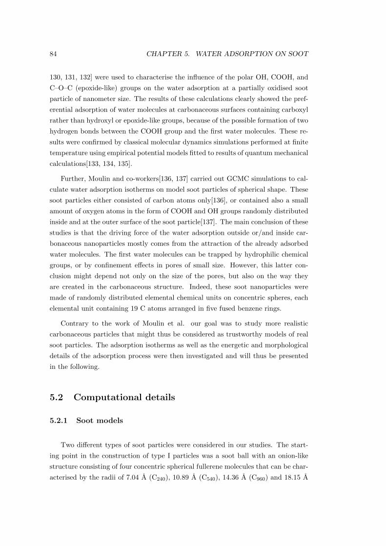
84 CHAPTER 5. WATER ADSORPTION ON SOOT
130, 131, 132] were used to characterise the influence of the polar OH, COOH, and
C–O–C (epoxide-like) groups on the water adsorption at a partially oxidised soot
particle of nanometer size. The results of these calculations clearly showed the pref-
erential adsorption of water molecules at carbonaceous surfaces containing carboxyl
rather than hydroxyl or epoxide-like groups, because of the possible formation of two
hydrogen bonds between the COOH group and the first water molecules. These re-
sults were confirmed by classical molecular dynamics simulations performed at finite
temperature using empirical potential models fitted to results of quantum mechanical
calculations[133, 134, 135].
Further, Moulin and co-workers[136, 137] carried out GCMC simulations to cal-
culate water adsorption isotherms on model soot particles of spherical shape. These
soot particles either consisted of carbon atoms only[136], or contained also a small
amount of oxygen atoms in the form of COOH and OH groups randomly distributed
inside and at the outer surface of the soot particle[137]. The main conclusion of these
studies is that the driving force of the water adsorption outside or/and inside car-
bonaceous nanoparticles mostly comes from the attraction of the already adsorbed
water molecules. The first water molecules can be trapped by hydrophilic chemical
groups, or by confinement effects in pores of small size. However, this latter con-
clusion might depend not only on the size of the pores, but also on the way they
are created in the carbonaceous structure. Indeed, these soot nanoparticles were
made of randomly distributed elemental chemical units on concentric spheres, each
elemental unit containing 19 C atoms arranged in five fused benzene rings.
Contrary to the work of Moulin et al. our goal was to study more realistic
carbonaceous particles that might thus be considered as trustworthy models of real
soot particles. The adsorption isotherms as well as the energetic and morphological
details of the adsorption process were then investigated and will thus be presented
in the following.
5.2 Computational details
5.2.1 Soot models
Two different types of soot particles were considered in our studies. The start-
ing point in the construction of type I particles was a soot ball with an onion-like
structure consisting of four concentric spherical fullerene molecules that can be char-
acterised by the radii of 7.04 A (C240), 10.89 A (C540), 14.36 A (C960) and 18.15 A
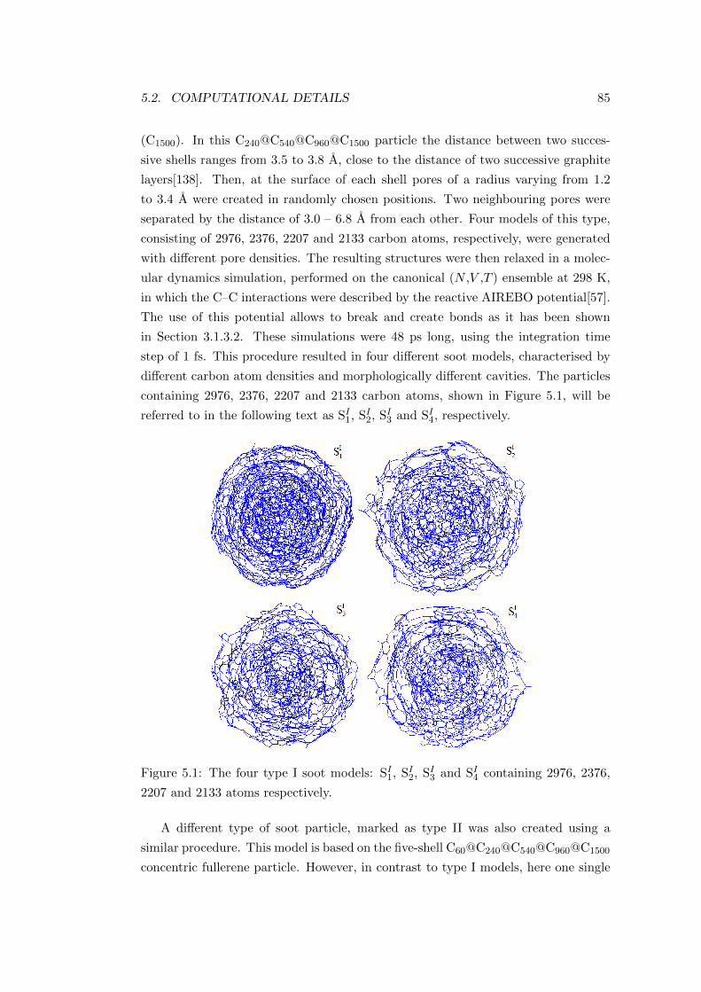
5.2. COMPUTATIONAL DETAILS 85
(C1500). In this C240@C540@C960@C1500 particle the distance between two succes-
sive shells ranges from 3.5 to 3.8 A, close to the distance of two successive graphite
layers[138]. Then, at the surface of each shell pores of a radius varying from 1.2
to 3.4 A were created in randomly chosen positions. Two neighbouring pores were
separated by the distance of 3.0 – 6.8 A from each other. Four models of this type,
consisting of 2976, 2376, 2207 and 2133 carbon atoms, respectively, were generated
with different pore densities. The resulting structures were then relaxed in a molec-
ular dynamics simulation, performed on the canonical (N ,V ,T ) ensemble at 298 K,
in which the C–C interactions were described by the reactive AIREBO potential[57].
The use of this potential allows to break and create bonds as it has been shown
in Section 3.1.3.2. These simulations were 48 ps long, using the integration time
step of 1 fs. This procedure resulted in four different soot models, characterised by
different carbon atom densities and morphologically different cavities. The particles
containing 2976, 2376, 2207 and 2133 carbon atoms, shown in Figure 5.1, will be
referred to in the following text as SI1, SI2, SI3 and SI4, respectively.
Figure 5.1: The four type I soot models: SI1, SI2, SI3 and SI4 containing 2976, 2376,
2207 and 2133 atoms respectively.
A different type of soot particle, marked as type II was also created using a
similar procedure. This model is based on the five-shell C60@C240@C540@C960@C1500
concentric fullerene particle. However, in contrast to type I models, here one single
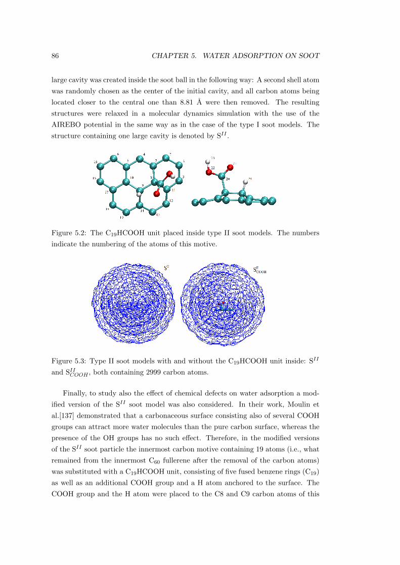
86 CHAPTER 5. WATER ADSORPTION ON SOOT
large cavity was created inside the soot ball in the following way: A second shell atom
was randomly chosen as the center of the initial cavity, and all carbon atoms being
located closer to the central one than 8.81 A were then removed. The resulting
structures were relaxed in a molecular dynamics simulation with the use of the
AIREBO potential in the same way as in the case of the type I soot models. The
structure containing one large cavity is denoted by SII .
Figure 5.2: The C19HCOOH unit placed inside type II soot models. The numbers
indicate the numbering of the atoms of this motive.
Figure 5.3: Type II soot models with and without the C19HCOOH unit inside: SII
and SIICOOH , both containing 2999 carbon atoms.
Finally, to study also the effect of chemical defects on water adsorption a mod-
ified version of the SII soot model was also considered. In their work, Moulin et
al.[137] demonstrated that a carbonaceous surface consisting also of several COOH
groups can attract more water molecules than the pure carbon surface, whereas the
presence of the OH groups has no such effect. Therefore, in the modified versions
of the SII soot particle the innermost carbon motive containing 19 atoms (i.e., what
remained from the innermost C60 fullerene after the removal of the carbon atoms)
was substituted with a C19HCOOH unit, consisting of five fused benzene rings (C19)
as well as an additional COOH group and a H atom anchored to the surface. The
COOH group and the H atom were placed to the C8 and C9 carbon atoms of this
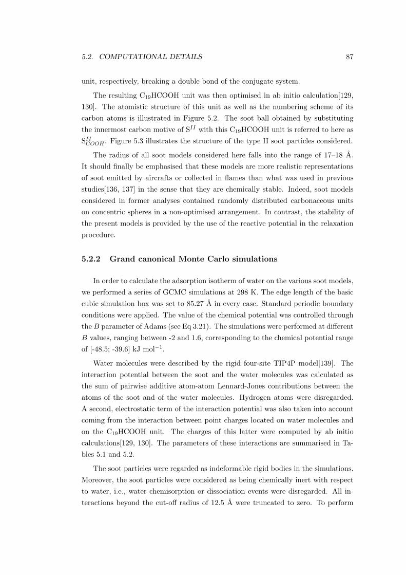
5.2. COMPUTATIONAL DETAILS 87
unit, respectively, breaking a double bond of the conjugate system.
The resulting C19HCOOH unit was then optimised in ab initio calculation[129,
130]. The atomistic structure of this unit as well as the numbering scheme of its
carbon atoms is illustrated in Figure 5.2. The soot ball obtained by substituting
the innermost carbon motive of SII with this C19HCOOH unit is referred to here as
SIICOOH . Figure 5.3 illustrates the structure of the type II soot particles considered.
The radius of all soot models considered here falls into the range of 17–18 A.
It should finally be emphasised that these models are more realistic representations
of soot emitted by aircrafts or collected in flames than what was used in previous
studies[136, 137] in the sense that they are chemically stable. Indeed, soot models
considered in former analyses contained randomly distributed carbonaceous units
on concentric spheres in a non-optimised arrangement. In contrast, the stability of
the present models is provided by the use of the reactive potential in the relaxation
procedure.
5.2.2 Grand canonical Monte Carlo simulations
In order to calculate the adsorption isotherm of water on the various soot models,
we performed a series of GCMC simulations at 298 K. The edge length of the basic
cubic simulation box was set to 85.27 A in every case. Standard periodic boundary
conditions were applied. The value of the chemical potential was controlled through
theB parameter of Adams (see Eq 3.21). The simulations were performed at different
B values, ranging between -2 and 1.6, corresponding to the chemical potential range
of [-48.5; -39.6] kJ mol−1.
Water molecules were described by the rigid four-site TIP4P model[139]. The
interaction potential between the soot and the water molecules was calculated as
the sum of pairwise additive atom-atom Lennard-Jones contributions between the
atoms of the soot and of the water molecules. Hydrogen atoms were disregarded.
A second, electrostatic term of the interaction potential was also taken into account
coming from the interaction between point charges located on water molecules and
on the C19HCOOH unit. The charges of this latter were computed by ab initio
calculations[129, 130]. The parameters of these interactions are summarised in Ta-
bles 5.1 and 5.2.
The soot particles were regarded as indeformable rigid bodies in the simulations.
Moreover, the soot particles were considered as being chemically inert with respect
to water, i.e., water chemisorption or dissociation events were disregarded. All in-
teractions beyond the cut-off radius of 12.5 A were truncated to zero. To perform
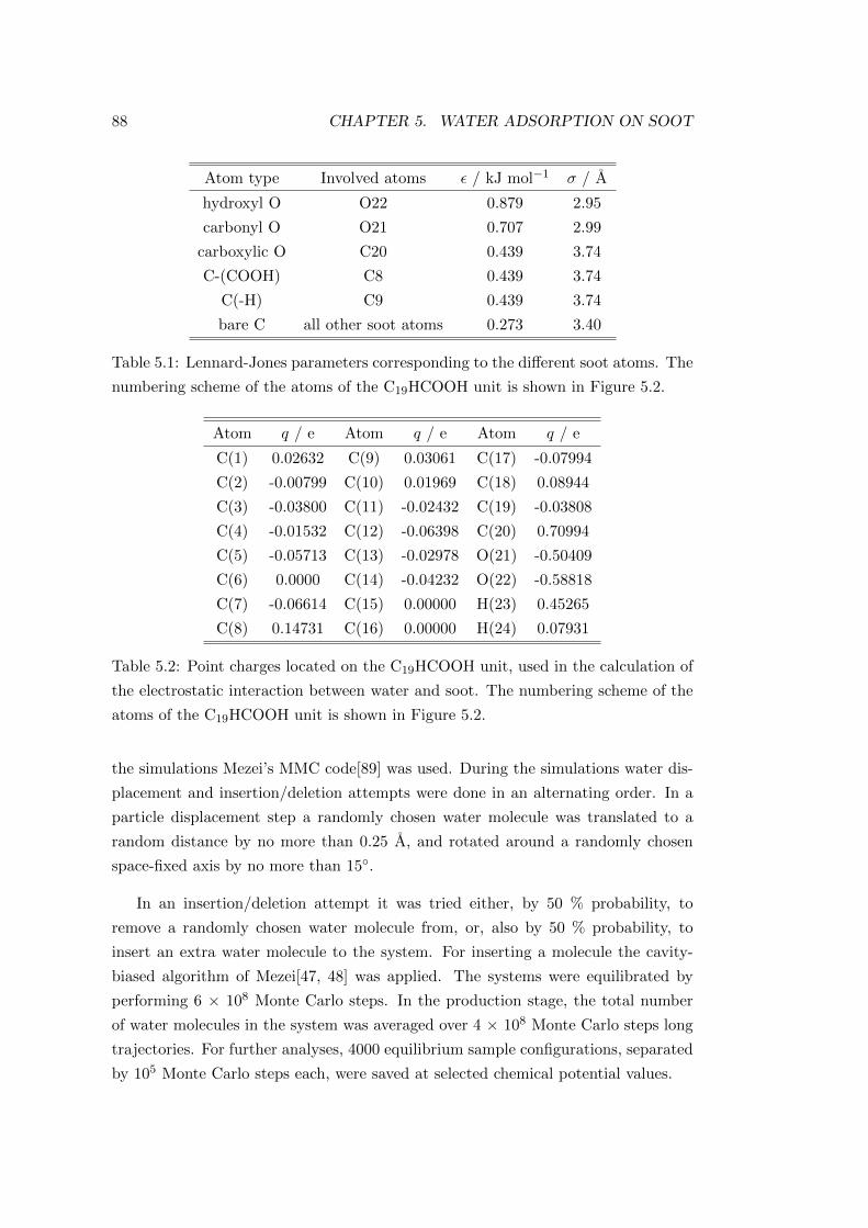
88 CHAPTER 5. WATER ADSORPTION ON SOOT
Atom type Involved atoms ε / kJ mol−1 σ / A
hydroxyl O O22 0.879 2.95
carbonyl O O21 0.707 2.99
carboxylic O C20 0.439 3.74
C-(COOH) C8 0.439 3.74
C(-H) C9 0.439 3.74
bare C all other soot atoms 0.273 3.40
Table 5.1: Lennard-Jones parameters corresponding to the different soot atoms. The
numbering scheme of the atoms of the C19HCOOH unit is shown in Figure 5.2.
Atom q / e Atom q / e Atom q / e
C(1) 0.02632 C(9) 0.03061 C(17) -0.07994
C(2) -0.00799 C(10) 0.01969 C(18) 0.08944
C(3) -0.03800 C(11) -0.02432 C(19) -0.03808
C(4) -0.01532 C(12) -0.06398 C(20) 0.70994
C(5) -0.05713 C(13) -0.02978 O(21) -0.50409
C(6) 0.0000 C(14) -0.04232 O(22) -0.58818
C(7) -0.06614 C(15) 0.00000 H(23) 0.45265
C(8) 0.14731 C(16) 0.00000 H(24) 0.07931
Table 5.2: Point charges located on the C19HCOOH unit, used in the calculation of
the electrostatic interaction between water and soot. The numbering scheme of the
atoms of the C19HCOOH unit is shown in Figure 5.2.
the simulations Mezei’s MMC code[89] was used. During the simulations water dis-
placement and insertion/deletion attempts were done in an alternating order. In a
particle displacement step a randomly chosen water molecule was translated to a
random distance by no more than 0.25 A, and rotated around a randomly chosen
space-fixed axis by no more than 15.
In an insertion/deletion attempt it was tried either, by 50 % probability, to
remove a randomly chosen water molecule from, or, also by 50 % probability, to
insert an extra water molecule to the system. For inserting a molecule the cavity-
biased algorithm of Mezei[47, 48] was applied. The systems were equilibrated by
performing 6 × 10⁸ Monte Carlo steps. In the production stage, the total number
of water molecules in the system was averaged over 4 × 10⁸ Monte Carlo steps long
trajectories. For further analyses, 4000 equilibrium sample configurations, separated
by 105 Monte Carlo steps each, were saved at selected chemical potential values.
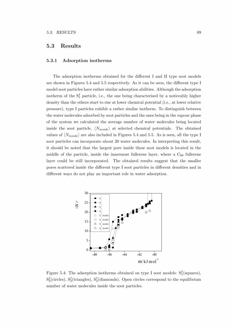
5.3. RESULTS 89
5.3 Results
5.3.1 Adsorption isotherms
The adsorption isotherms obtained for the different I and II type soot models
are shown in Figures 5.4 and 5.5 respectively. As it can be seen, the different type I
model soot particles have rather similar adsorption abilities. Although the adsorption
isotherm of the SI1 particle, i.e., the one being characterised by a noticeably higher
density than the others start to rise at lower chemical potential (i.e., at lower relative
pressure), type I particles exhibit a rather similar isotherm. To distinguish between
the water molecules adsorbed by soot particles and the ones being in the vapour phase
of the system we calculated the average number of water molecules being located
inside the soot particle, 〈Ninside〉 at selected chemical potentials. The obtained
values of 〈Ninside〉 are also included in Figures 5.4 and 5.5. As is seen, all the type I
soot particles can incorporate about 20 water molecules. In interpreting this result,
it should be noted that the largest pore inside these soot models is located in the
middle of the particle, inside the innermost fullerene layer, where a C60 fullerene
layer could be still incorporated. The obtained results suggest that the smaller
pores scattered inside the different type I soot particles in different densities and in
different ways do not play an important role in water adsorption.
-48 -46 -44 -42 -400
5
10
15
20
25
30
µ / kJ mol-1
<N>
S1
I
S2
I
S3
I
S4
I
S1
I inside
S2
I inside
S3
I inside
S4
I inside
Figure 5.4: The adsorption isotherms obtained on type I soot models: SI1(squares),
SI2(circles), SI3(triangles), SI4(diamonds). Open circles correspond to the equilibrium
number of water molecules inside the soot particles.
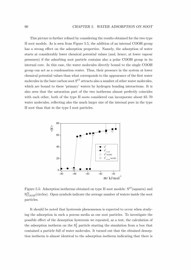
90 CHAPTER 5. WATER ADSORPTION ON SOOT
This picture is further refined by considering the results obtained for the two type
II soot models. As is seen from Figure 5.5, the addition of an internal COOH group
has a strong effect on the adsorption properties. Namely, the adsorption of water
starts at considerably lower chemical potential values (and, hence, at lower vapour
pressures) if the adsorbing soot particle contains also a polar COOH group in its
internal core. In this case, the water molecules directly bound to the single COOH
group can act as a condensation center. Thus, their presence in the system at lower
chemical potential values than what corresponds to the appearance of the first water
molecules in the bare carbon soot SII attracts also a number of other water molecules,
which are bound to these ‘primary’ waters by hydrogen bonding interactions. It is
also seen that the saturation part of the two isotherms almost perfectly coincides
with each other, both of the type II soots considered can incorporate about 65–70
water molecules, reflecting also the much larger size of the internal pore in the type
II soot than that in the type I soot particles.
-45 -44 -43 -42 -410
20
40
60
80
<N>
µ / kJ mol-1
SII
SII
COOH
SII inside
SII
COOH inside
Figure 5.5: Adsorption isotherms obtained on type II soot models: SII(squares) and
SIICOOH(circles). Open symbols indicate the average number of waters inside the soot
particles.
It should be noted that hysteresis phenomenon is expected to occur when study-
ing the adsorption in such a porous media as our soot particles. To investigate the
possible effect of the desorption hysteresis we repeated, as a test, the calculation of
the adsorption isotherm on the SI2 particle starting the simulation from a box that
contained a particle full of water molecules. It turned out that the obtained desorp-
tion isotherm is almost identical to the adsorption isotherm indicating that there is
5.3. RESULTS 91
no significant hysteresis related to water adsorption on this kind of soot particles.
The obtained results suggest that two possible factors might determine the ad-
sorption ability of the different soot particles. First, the size and shape of the pore
plays an important role in this respect. It is clear that the main driving force of
water adsorption in large apolar carriers, such as soot balls is the water–water inter-
action, i.e., the possibility of hydrogen bond formation with already adsorbed water
molecules[136, 137]. Therefore, adsorbing pores should be large enough, and their
shape should be sufficiently compact to host a large enough water cluster the mole-
cules of which can form a sufficient number of hydrogen bonds to stabilise themselves
in the apolar environment. If the pore is too small or it is simply too narrow then the
number of hydrogen bonded neighbours of the water molecules is limited by these
geometric constraints. In this case, the energy gain of the adsorbed water molecules
might not overcompensate the effect of the entropy loss accompanying their cluster-
ing, which prevents their adsorption. This seems to be the case in the smaller pores
of the type I soot particles. Further, the amount of water a soot particle can adsorb
is obviously related to the size of the pore inside the soot.
On the other hand, water–water interaction can only lead to the adsorption
of new water molecules if the soot already contains at least some traces of water.
Thus, the second possible factor that might determine adsorption is the ability of
the soot particle of attracting the first few water molecules. In other words, the
pores inside the soot might contain a few adsorption sites at which water molecules
can be particularly strongly bound even in the absence of other water molecules. In
this case, these first adsorbed waters can act as nucleation centers for the adsorption
at higher chemical potential values. This effect is clearly demonstrated in the case
of the type II soot particles, where the optimal location of the first adsorbed water
molecules can indeed initiate the adsorption of other water molecules, and it is also
likely to be the factor responsible for the fact that the adsorption isotherms obtained
on the different type I soot particles start at somewhat different chemical potentials.
In order to investigate the impact of these two factors, i.e., the role of the optimal
pore shape and of the optimal location of the first adsorbed molecules, in the follow-
ing we analyse in detail the position of the first adsorbed molecules inside the various
soot balls, the morphological properties of the pores in our various soot models, and
the energetic background of the adsorption process investigated.
5.3.2 Position of the first adsorbed molecules
In order to investigate the role of the position of the first few adsorbed water
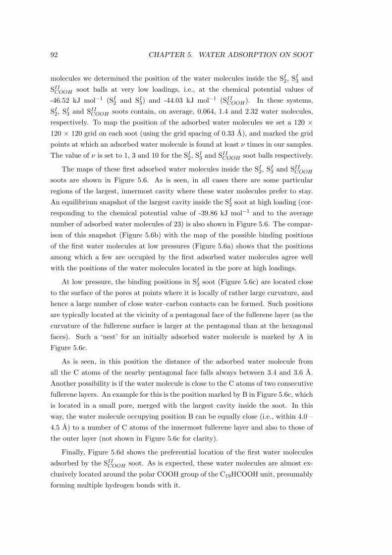
92 CHAPTER 5. WATER ADSORPTION ON SOOT
molecules we determined the position of the water molecules inside the SI2, SI3 and
SIICOOH soot balls at very low loadings, i.e., at the chemical potential values of
-46.52 kJ mol−1 (SI2 and SI3) and -44.03 kJ mol−1 (SIICOOH). In these systems,
SI2, SI3 and SIICOOH soots contain, on average, 0.064, 1.4 and 2.32 water molecules,
respectively. To map the position of the adsorbed water molecules we set a 120 ×120 × 120 grid on each soot (using the grid spacing of 0.33 A), and marked the grid
points at which an adsorbed water molecule is found at least ν times in our samples.
The value of ν is set to 1, 3 and 10 for the SI2, SI3 and SIICOOH soot balls respectively.
The maps of these first adsorbed water molecules inside the SI2, SI3 and SIICOOHsoots are shown in Figure 5.6. As is seen, in all cases there are some particular
regions of the largest, innermost cavity where these water molecules prefer to stay.
An equilibrium snapshot of the largest cavity inside the SI2 soot at high loading (cor-
responding to the chemical potential value of -39.86 kJ mol−1 and to the average
number of adsorbed water molecules of 23) is also shown in Figure 5.6. The compar-
ison of this snapshot (Figure 5.6b) with the map of the possible binding positions
of the first water molecules at low pressures (Figure 5.6a) shows that the positions
among which a few are occupied by the first adsorbed water molecules agree well
with the positions of the water molecules located in the pore at high loadings.
At low pressure, the binding positions in SI3 soot (Figure 5.6c) are located close
to the surface of the pores at points where it is locally of rather large curvature, and
hence a large number of close water–carbon contacts can be formed. Such positions
are typically located at the vicinity of a pentagonal face of the fullerene layer (as the
curvature of the fullerene surface is larger at the pentagonal than at the hexagonal
faces). Such a ‘nest’ for an initially adsorbed water molecule is marked by A in
Figure 5.6c.
As is seen, in this position the distance of the adsorbed water molecule from
all the C atoms of the nearby pentagonal face falls always between 3.4 and 3.6 A.
Another possibility is if the water molecule is close to the C atoms of two consecutive
fullerene layers. An example for this is the position marked by B in Figure 5.6c, which
is located in a small pore, merged with the largest cavity inside the soot. In this
way, the water molecule occupying position B can be equally close (i.e., within 4.0 –
4.5 A) to a number of C atoms of the innermost fullerene layer and also to those of
the outer layer (not shown in Figure 5.6c for clarity).
Finally, Figure 5.6d shows the preferential location of the first water molecules
adsorbed by the SIICOOH soot. As is expected, these water molecules are almost ex-
clusively located around the polar COOH group of the C19HCOOH unit, presumably
forming multiple hydrogen bonds with it.
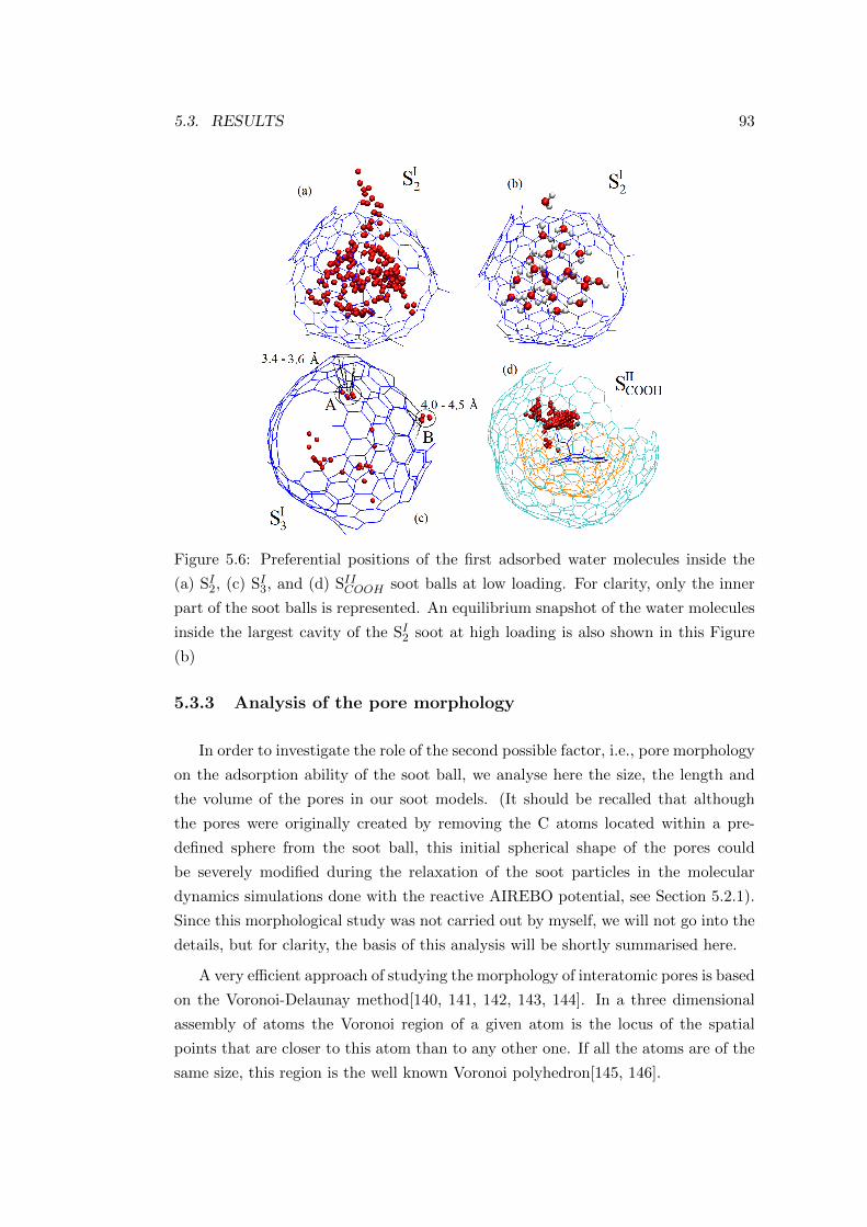
5.3. RESULTS 93
Figure 5.6: Preferential positions of the first adsorbed water molecules inside the
(a) SI2, (c) SI3, and (d) SIICOOH soot balls at low loading. For clarity, only the inner
part of the soot balls is represented. An equilibrium snapshot of the water molecules
inside the largest cavity of the SI2 soot at high loading is also shown in this Figure
(b)
5.3.3 Analysis of the pore morphology
In order to investigate the role of the second possible factor, i.e., pore morphology
on the adsorption ability of the soot ball, we analyse here the size, the length and
the volume of the pores in our soot models. (It should be recalled that although
the pores were originally created by removing the C atoms located within a pre-
defined sphere from the soot ball, this initial spherical shape of the pores could
be severely modified during the relaxation of the soot particles in the molecular
dynamics simulations done with the reactive AIREBO potential, see Section 5.2.1).
Since this morphological study was not carried out by myself, we will not go into the
details, but for clarity, the basis of this analysis will be shortly summarised here.
A very efficient approach of studying the morphology of interatomic pores is based
on the Voronoi-Delaunay method[140, 141, 142, 143, 144]. In a three dimensional
assembly of atoms the Voronoi region of a given atom is the locus of the spatial
points that are closer to this atom than to any other one. If all the atoms are of the
same size, this region is the well known Voronoi polyhedron[145, 146].
94 CHAPTER 5. WATER ADSORPTION ON SOOT
The Voronoi regions constructed for all atoms constitute a tessellation, namely
a decomposition of the space without gaps and overlaps. The edges and vertices of
the Voronoi regions pertinent to this tessellation constitute a network (called the
Voronoi network). Edges and vertices of the Voronoi network are the loci of points
that are equally far from the nearest three and four atoms, respectively. Thus,
each vertex of the Voronoi network corresponds to a quadruplet of four mutually
neighboring atoms, whose particular feature is that the inscribed sphere between
them is empty, i.e., does not overlap with any atoms of the system. Such a quadruplet
of atoms determines a tetrahedron, called the Delaunay simplex. Thus, the Delaunay
simplices represent the simplest cavities located between the atoms, and any complex
pore can be considered as a cluster of such simplices.
Further, each edge of the Voronoi network represents a fairway passing through
the narrow bottleneck between three atoms from one vertex to the neighbouring
one. These features make the Voronoi network a very convenient tool for analysis of
pores. Once this network is determined, the properties of the corresponding pores
can be easily analysed[142, 143]. Algorithms and programs for constructing the
Voronoi network can easily be found for the special case of uniform atom size[149],
whereas for the general case of atoms of different radii such an algorithm was recently
published[150]. It should be noted that our models consist of C atoms of uniform
size, with the exception of the two O atoms of the C19HCOOH units present in
the SIICOOH soot model. (Since the H atoms do not carry Lennard-Jones interaction
centers, they are also neglected in this analysis).
A physically meaningful way of defining pores is to regard regions of the empty
interatomic space that is accessible for a spherical probe of the pre-defined radius
Rprobe. Here we set Rprobe to be 1.4 A, corresponding roughly to the size of a water O
atom. In this way, regions of the empty space between the soot C atoms that are ac-
cessible for a single water molecule are considered as pores. Thus, interstitial spheres
(determined by the Delaunay simplices) with the radius larger than 1.4 A correspond
to the simplicial cavities accessible for our probe. Further, if the bottleneck radius
between two such neighbouring simplicial cavities is also larger than 1.4 A, both of
them are included in the same cluster, and hence belong to the same complex pore.
In this way, all the pores accessible for a water molecule can be detected. Such a
pore can be described either as a cluster of the corresponding Delaunay simplices,
or as an aggregate of the (usually strongly overlapping) interstitial spheres, or by
the list of the surrounding atoms. The largest pores inside the five bare carbon soot
models considered are shown in Figure 5.7 as an assemble of empty spheres with
radii of at least 1.4 A (the pore inside the SIICOOH soot particle is not shown here
5.3. RESULTS 95
since it looks almost indistinguishable from that in the SII particle).
Figure 5.7: The largest pores represented by the combination of empty spheres
inscribed into the 5 bare carbon soot particles considered here as is resulted form the
Voronoi analysis. Different colours correspond to different radii from blue (smallest
one) to red (largest one).
In analysing the morphology of the interatomic pores in our soot models we
calculated the following characteristics. The volume of a pore V is calculated as the
sum of the empty volume of the corresponding Delaunay simplices. Pores can also
be characterised by the radius of the largest interstitial sphere (simplicial cavity)
belonging to them, Rmax, and by their length (i.e., the largest distance between
two points inside the corresponding aggregate of simplicial cavities), L. In the pore
morphology analysis we take into account only the largest pore in each of the six
soot particles considered.
The values of V , Rmax, and L corresponding to the different soot models are
summarised in Table 5.3. This table also contains the estimated maximum number
of water molecules that could be incorporated in the largest pore and in the largest
spherical cavity, Nmax and Nsp, respectively (assuming the experimental number
density of liquid water of 0.0334 A−1), and the average number of water molecules
found to be adsorbed inside the soot at the highest loading, 〈N〉ads. As is seen, the
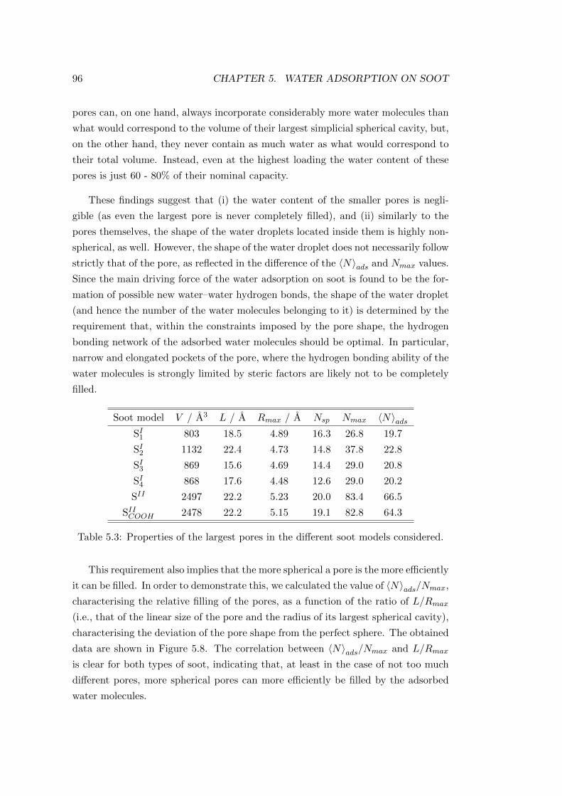
96 CHAPTER 5. WATER ADSORPTION ON SOOT
pores can, on one hand, always incorporate considerably more water molecules than
what would correspond to the volume of their largest simplicial spherical cavity, but,
on the other hand, they never contain as much water as what would correspond to
their total volume. Instead, even at the highest loading the water content of these
pores is just 60 - 80% of their nominal capacity.
These findings suggest that (i) the water content of the smaller pores is negli-
gible (as even the largest pore is never completely filled), and (ii) similarly to the
pores themselves, the shape of the water droplets located inside them is highly non-
spherical, as well. However, the shape of the water droplet does not necessarily follow
strictly that of the pore, as reflected in the difference of the 〈N〉ads and Nmax values.
Since the main driving force of the water adsorption on soot is found to be the for-
mation of possible new water–water hydrogen bonds, the shape of the water droplet
(and hence the number of the water molecules belonging to it) is determined by the
requirement that, within the constraints imposed by the pore shape, the hydrogen
bonding network of the adsorbed water molecules should be optimal. In particular,
narrow and elongated pockets of the pore, where the hydrogen bonding ability of the
water molecules is strongly limited by steric factors are likely not to be completely
filled.
Soot model V / A3 L / A Rmax / A Nsp Nmax 〈N〉adsSI1 803 18.5 4.89 16.3 26.8 19.7
SI2 1132 22.4 4.73 14.8 37.8 22.8
SI3 869 15.6 4.69 14.4 29.0 20.8
SI4 868 17.6 4.48 12.6 29.0 20.2
SII 2497 22.2 5.23 20.0 83.4 66.5
SIICOOH 2478 22.2 5.15 19.1 82.8 64.3
Table 5.3: Properties of the largest pores in the different soot models considered.
This requirement also implies that the more spherical a pore is the more efficiently
it can be filled. In order to demonstrate this, we calculated the value of 〈N〉ads/Nmax,
characterising the relative filling of the pores, as a function of the ratio of L/Rmax
(i.e., that of the linear size of the pore and the radius of its largest spherical cavity),
characterising the deviation of the pore shape from the perfect sphere. The obtained
data are shown in Figure 5.8. The correlation between 〈N〉ads/Nmax and L/Rmax
is clear for both types of soot, indicating that, at least in the case of not too much
different pores, more spherical pores can more efficiently be filled by the adsorbed
water molecules.
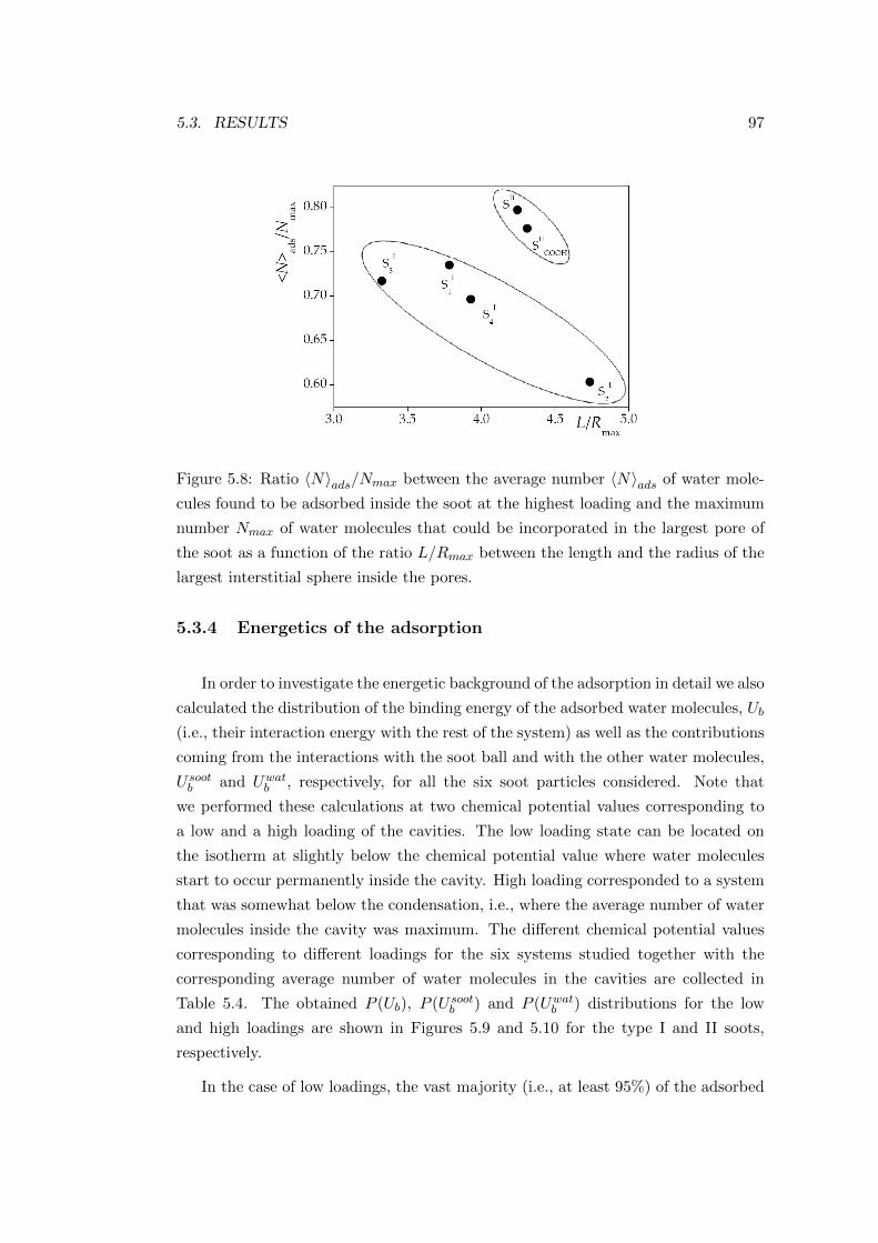
5.3. RESULTS 97
Figure 5.8: Ratio 〈N〉ads/Nmax between the average number 〈N〉ads of water mole-
cules found to be adsorbed inside the soot at the highest loading and the maximum
number Nmax of water molecules that could be incorporated in the largest pore of
the soot as a function of the ratio L/Rmax between the length and the radius of the
largest interstitial sphere inside the pores.
5.3.4 Energetics of the adsorption
In order to investigate the energetic background of the adsorption in detail we also
calculated the distribution of the binding energy of the adsorbed water molecules, Ub
(i.e., their interaction energy with the rest of the system) as well as the contributions
coming from the interactions with the soot ball and with the other water molecules,
U sootb and Uwatb , respectively, for all the six soot particles considered. Note that
we performed these calculations at two chemical potential values corresponding to
a low and a high loading of the cavities. The low loading state can be located on
the isotherm at slightly below the chemical potential value where water molecules
start to occur permanently inside the cavity. High loading corresponded to a system
that was somewhat below the condensation, i.e., where the average number of water
molecules inside the cavity was maximum. The different chemical potential values
corresponding to different loadings for the six systems studied together with the
corresponding average number of water molecules in the cavities are collected in
Table 5.4. The obtained P (Ub), P (U sootb ) and P (Uwatb ) distributions for the low
and high loadings are shown in Figures 5.9 and 5.10 for the type I and II soots,
respectively.
In the case of low loadings, the vast majority (i.e., at least 95%) of the adsorbed
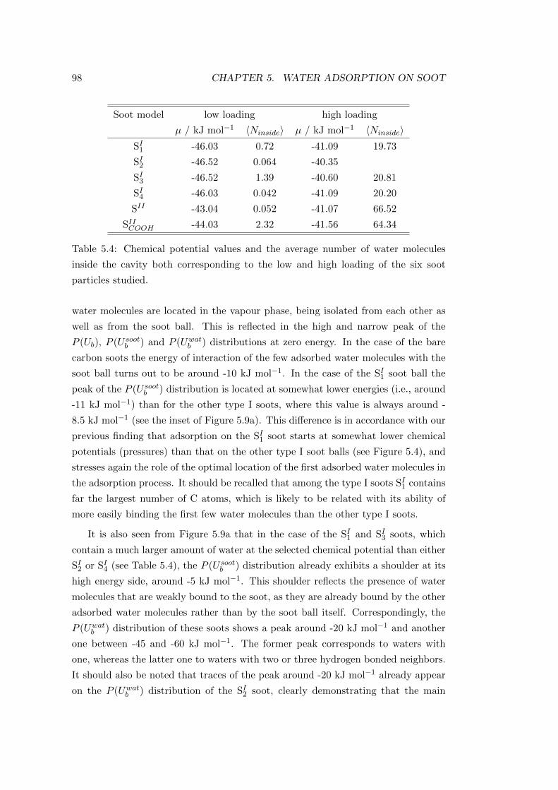
98 CHAPTER 5. WATER ADSORPTION ON SOOT
Soot model low loading high loading
µ / kJ mol−1 〈Ninside〉 µ / kJ mol−1 〈Ninside〉SI1 -46.03 0.72 -41.09 19.73
SI2 -46.52 0.064 -40.35
SI3 -46.52 1.39 -40.60 20.81
SI4 -46.03 0.042 -41.09 20.20
SII -43.04 0.052 -41.07 66.52
SIICOOH -44.03 2.32 -41.56 64.34
Table 5.4: Chemical potential values and the average number of water molecules
inside the cavity both corresponding to the low and high loading of the six soot
particles studied.
water molecules are located in the vapour phase, being isolated from each other as
well as from the soot ball. This is reflected in the high and narrow peak of the
P (Ub), P (U sootb ) and P (Uwatb ) distributions at zero energy. In the case of the bare
carbon soots the energy of interaction of the few adsorbed water molecules with the
soot ball turns out to be around -10 kJ mol−1. In the case of the SI1 soot ball the
peak of the P (U sootb ) distribution is located at somewhat lower energies (i.e., around
-11 kJ mol−1) than for the other type I soots, where this value is always around -
8.5 kJ mol−1 (see the inset of Figure 5.9a). This difference is in accordance with our
previous finding that adsorption on the SI1 soot starts at somewhat lower chemical
potentials (pressures) than that on the other type I soot balls (see Figure 5.4), and
stresses again the role of the optimal location of the first adsorbed water molecules in
the adsorption process. It should be recalled that among the type I soots SI1 contains
far the largest number of C atoms, which is likely to be related with its ability of
more easily binding the first few water molecules than the other type I soots.
It is also seen from Figure 5.9a that in the case of the SI1 and SI3 soots, which
contain a much larger amount of water at the selected chemical potential than either
SI2 or SI4 (see Table 5.4), the P (U sootb ) distribution already exhibits a shoulder at its
high energy side, around -5 kJ mol−1. This shoulder reflects the presence of water
molecules that are weakly bound to the soot, as they are already bound by the other
adsorbed water molecules rather than by the soot ball itself. Correspondingly, the
P (Uwatb ) distribution of these soots shows a peak around -20 kJ mol−1 and another
one between -45 and -60 kJ mol−1. The former peak corresponds to waters with
one, whereas the latter one to waters with two or three hydrogen bonded neighbors.
It should also be noted that traces of the peak around -20 kJ mol−1 already appear
on the P (Uwatb ) distribution of the SI2 soot, clearly demonstrating that the main
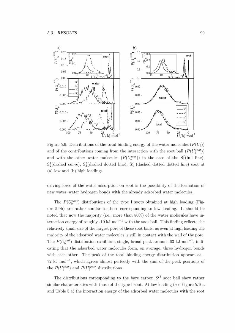
5.3. RESULTS 99
S1
I
S2
I
S3
I
S4
I
total
b)
water
soot
Figure 5.9: Distributions of the total binding energy of the water molecules (P (Ub))
and of the contributions coming from the interaction with the soot ball (P (U sootb ))
and with the other water molecules (P (Uwatb )) in the case of the SI1(full line),
SI2(dashed curve), SI3(dashed dotted line), SI4 (dashed dotted dotted line) soot at
(a) low and (b) high loadings.
driving force of the water adsorption on soot is the possibility of the formation of
new water–water hydrogen bonds with the already adsorbed water molecules.
The P (U sootb ) distributions of the type I soots obtained at high loading (Fig-
ure 5.9b) are rather similar to those corresponding to low loading. It should be
noted that now the majority (i.e., more than 80%) of the water molecules have in-
teraction energy of roughly -10 kJ mol−1 with the soot ball. This finding reflects the
relatively small size of the largest pore of these soot balls, as even at high loading the
majority of the adsorbed water molecules is still in contact with the wall of the pore.
The P (Uwatb ) distribution exhibits a single, broad peak around -63 kJ mol−1, indi-
cating that the adsorbed water molecules form, on average, three hydrogen bonds
with each other. The peak of the total binding energy distribution appears at -
72 kJ mol−1, which agrees almost perfectly with the sum of the peak positions of
the P (U sootb ) and P (Uwatb ) distributions.
The distributions corresponding to the bare carbon SII soot ball show rather
similar characteristics with those of the type I soot. At low loading (see Figure 5.10a
and Table 5.4) the interaction energy of the adsorbed water molecules with the soot
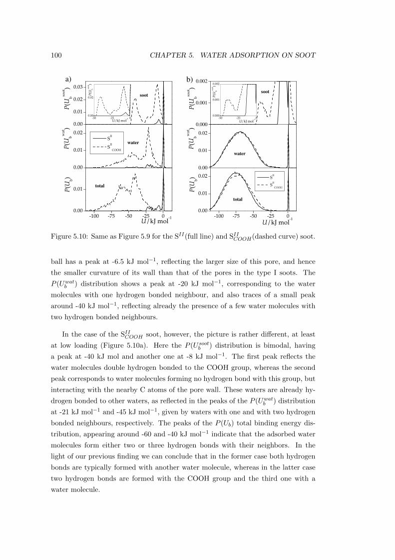
100 CHAPTER 5. WATER ADSORPTION ON SOOT
soot
water
total
a)
0.000
0.001
0.002
soot
0.00
0.01
0.02
water
total
b)
Figure 5.10: Same as Figure 5.9 for the SII(full line) and SIICOOH(dashed curve) soot.
ball has a peak at -6.5 kJ mol−1, reflecting the larger size of this pore, and hence
the smaller curvature of its wall than that of the pores in the type I soots. The
P (Uwatb ) distribution shows a peak at -20 kJ mol−1, corresponding to the water
molecules with one hydrogen bonded neighbour, and also traces of a small peak
around -40 kJ mol−1, reflecting already the presence of a few water molecules with
two hydrogen bonded neighbours.
In the case of the SIICOOH soot, however, the picture is rather different, at least
at low loading (Figure 5.10a). Here the P (U sootb ) distribution is bimodal, having
a peak at -40 kJ mol and another one at -8 kJ mol−1. The first peak reflects the
water molecules double hydrogen bonded to the COOH group, whereas the second
peak corresponds to water molecules forming no hydrogen bond with this group, but
interacting with the nearby C atoms of the pore wall. These waters are already hy-
drogen bonded to other waters, as reflected in the peaks of the P (Uwatb ) distribution
at -21 kJ mol−1 and -45 kJ mol−1, given by waters with one and with two hydrogen
bonded neighbours, respectively. The peaks of the P (Ub) total binding energy dis-
tribution, appearing around -60 and -40 kJ mol−1 indicate that the adsorbed water
molecules form either two or three hydrogen bonds with their neighbors. In the
light of our previous finding we can conclude that in the former case both hydrogen
bonds are typically formed with another water molecule, whereas in the latter case
two hydrogen bonds are formed with the COOH group and the third one with a
water molecule.
5.4. CONCLUSION 101
The differences between the bare carbon SII and the COOH-containing SIICOOHsoots, however, disappear at high loading (see Figure 5.10b), in accordance with our
previous finding that the role of the polar COOH group is limited to the initiation
of the adsorption at low pressures. Here, the amplitude of the peak of the P (U sootb )
distribution of the SIICOOH soot at -40 kJ mol−1 is an order of magnitude smaller
than that at low loading, as hydrogen bonding with the COOH group now involves
only a small minority of the adsorbed water molecules. Further, the majority of the
waters (also not such a large fraction as in the case of the type I soots) are still in
contact with the pore wall, and they form, on average, three hydrogen bonds with
each other, irrespective of whether the soot contains a polar COOH group or not.
5.4 Conclusion
In this chapter we have presented a study on the adsorption process of water on
chemically stable model soot particles by means of the grand canonical Monte Carlo
method, and related the characteristics of the pores inside the soot ball with their
adsorption ability. The obtained results clearly show that the main driving force of
water adsorption on soot is the formation of new possible hydrogen bonds with the
already adsorbed water molecules. We found that there are two important factors
influencing the adsorption ability of soot. The first of these factors is the ability of
the soot of accommodating the first adsorbed water molecules. Since the presence
of these molecules initiates the adsorption of other waters, the stronger these first
water molecules can be bound by the soot, the earlier starts the adsorption. This
can be achieved when strong hydrophilic sites are present in the soot. Furthermore,
higher soot density may also result in the enhanced affinity of water molecules for
being accomodated in soot cavities.
The other factor concerns morphological characteristics, primarily size and shape
of the pores. In general, adsorbing pores should be such that the hydrogen bonding
network of the water molecules filling them should be optimal. It turned out that
this requirement practically means that water molecules should be able to form, on
average, at least three hydrogen bonds with each other. This implies that too small
pores as well as narrow and deep pockets of the larger pores are not filled with water
even at high pressures. Although the adsorbed water droplet is found not to be
spherical, it turned out that, in general, more spherical pores can be more efficiently
filled with water at high loading.
It is also clear that the size of the pores is a crucial factor of the adsorption.
102 CHAPTER 5. WATER ADSORPTION ON SOOT
Thus, smaller pores meet better with the first criterion, as the first adsorbed water
molecules can interact stronger with the nearby C atoms of the soot in a small
pore of highly curved wall. On the other hand, such pores satisfy less the second
criterion, as the hydrogen bonding network of water filling smaller pores is more
strongly restricted by steric factors. Our results thus suggest that there might be an
optimal range of pore sizes in soots which corresponds to the best water adsorption
ability of the soot, i.e., when it is able to bind a noticeable amount of water even at
rather low pressures.
Note that although we investigated only soot micropores in our study, the results
allow us to extend our conclusions to the interpretation of the stepwise structure of
an experimental isotherm obtained on kerosene soot (see Figure 2.3). The distinct
steps can thus be attributed to the gradual filling-up of the adsorption sites (pores
and pockets) being characterised (as we have seen form this study) by either different
size and shape or different amount of oxygenated functional (mainly COOH) groups.
Note that such a comparative GCMC study may reveal a lot of details of such a
complex process like the adsorption of water molecules on soot.

Chapter 6
Reactivity of soot particles
6.1 Introduction
In this chapter we present results concerning the effect of soot particles on the
atmospheric oxidation reaction of PAHs by OH. PAH molecules have a high affinity
for carbonaceous materials, thus the adsorption of PAHs on soot may influence their
abundance in the gas phase, and also their atmospheric chemistry[151].
Soot particles are difficult to characterise from a physico-chemical point of view,
as we have seen in Section 2.4.2. Their structure may be very diverse, their surface
may be oxidised to a certain extent, and they might be associated with organic and
inorganic materials at their surface. These result in the fact that soot is not a well-
defined chemical substance[152]. As a consequence, studies of the physico-chemistry
of PAHs on soot surfaces are very scarce.
Up to now, there have only been a limited number of controlled laboratory[153,
154] or field [155, 156] studies on the adsorption of PAHs onto soot, and, to our best
knowledge, there is only one paper devoted to the experimental study of the uptake
of aromatic hydrocarbons onto soot with a known surface area, as a function of tem-
perature and partial pressure[11]. In their study, Esteve et al.[157] characterised the
role of OH, NO2 and NO radicals on the reactivity of 11 polyaromatic compounds
adsorbed on graphite particles chosen as a model of atmospheric carbonaceous par-
ticles. In this study, all PAHs presented similar rate constants while reacting with
OH, and, compared to the reactivity in the gas phase, the heterogeneous reaction
with OH radicals seems to show a potential inhibiting effect of the graphite surface,
meaning that the mechanisms may be sensibly different[157].
Only a few theoretical studies have been devoted to the structural and energetic
103
104 CHAPTER 6. REACTIVITY OF SOOT PARTICLES
characterisation of the interactions between PAHs and carbonaceous surfaces like
soot, primarily due to the fact that these systems are too large for tractable ab
initio calculations. Indeed, a realistic theoretical simulation of intermolecular forces
requires high-level electronic quantum calculations to account for dispersion effects.
The term ‘high-level quantum calculation’ refers to the use of very large basis sets
and a precise description of the correlation energy. Even for a simple perturbative
approach, double excitations on two interacting molecules are necessary to mimic
dispersion effects. Large basis sets are also necessary to minimise both the basis set
convergence error and the basis set superposition error. Such high-level calculations
require a great amount of computational resources[158], and, as a consequence, they
can only be done for small systems, such as the benzene dimer[159].
Gonzalez and co-workers[160, 161] proposed a method called the Hartree-Fock
Dispersion model (HFD) to calculate the structure and binding energy of aromatic
clusters, following the work originally proposed by Hepburn et al.[162]. In this HFD
method, the calculation of the intermolecular energies combines an ab initio self-
consistent field (SCF) interaction energy with an empirical dispersion energy term
described by the London theory that provides a very efficient analytical approach
to account for dispersion effect[160]. The method was successfully used to describe
dimers of benzene, naphthalene, anthracene and pyrene, as well as the naphtha-
lene trimer[161]. However, even this simplified method is unable to handle large
soot/PAH systems.
Collignon et al. have developed a new method[163, 164], which is applicable
for large systems. The so-called semi-empirical-dispersion (SE-D) method, com-
bines the semi-empirical description of the electrostatic and induction interactions
with a sum of two-body London dispersion terms proportional to R−6 (R being the
distance)[163].
In my work, this new method was used to describe the interaction between a
PAH molecule and soot. This latter was replaced by a model particle as it is simpler
and better characterised than real soot. The model particle was chosen to be a large
graphene-like molecule consisting of fused benzene rings and having hydrogens only
at the boundaries to eliminate free valences. It should be noted that a real soot
surface is likely oxidised, and hence contains oxygenated functional groups, which
may influence the chemistry of PAH molecules. But, as a first step, a large, flat and
perfect carbonaceous surface was studied.
To investigate the oxidation reaction of benzene, naphthalene and anthracene by
OH radical in the gas phase as compared to that occuring on a graphene surface, I
used a new kinetic-statistical approach aiming at catching the differencies between
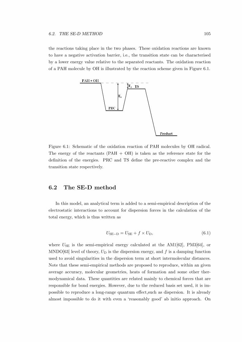
6.2. THE SE-D METHOD 105
the reactions taking place in the two phases. These oxidation reactions are known
to have a negative activation barrier, i.e., the transition state can be characterised
by a lower energy value relative to the separated reactants. The oxidation reaction
of a PAH molecule by OH is illustrated by the reaction scheme given in Figure 6.1.
Figure 6.1: Schematic of the oxidation reaction of PAH molecules by OH radical.
The energy of the reactants (PAH + OH) is taken as the reference state for the
definition of the energies. PRC and TS define the pre-reactive complex and the
transition state respectively.
6.2 The SE-D method
In this model, an analytical term is added to a semi-empirical description of the
electrostatic interactions to account for dispersion forces in the calculation of the
total energy, which is thus written as
USE−D = USE + f × UD, (6.1)
where USE is the semi-empirical energy calculated at the AM1[62], PM3[64], or
MNDO[63] level of theory, UD is the dispersion energy, and f is a damping function
used to avoid singularities in the dispersion term at short intermolecular distances.
Note that these semi-empirical methods are proposed to reproduce, within an given
average accuracy, molecular geometries, heats of formation and some other ther-
modynamical data. These quantities are related mainly to chemical forces that are
responsible for bond energies. However, due to the reduced basis set used, it is im-
possible to reproduce a long-range quantum effect,such as dispersion. It is already
almost impossible to do it with even a ‘reasonably good’ ab initio approach. On
106 CHAPTER 6. REACTIVITY OF SOOT PARTICLES
the contrary, long-range electrostatic and induction effects are included in a more or
less realistic way in the calculations by the SCF procedure itself. It turns out that
the introduction of a sum of R−6 terms added at long distance to the SCF energy
appears as an elegant way to include dispersion, even if it requires some ‘savoir-faire’
for the estimation of these terms.
The dispersion contribution to the total energy is thus expressed as[165]
f × UD = −Ng∑i=1
Np∑j=1
1
(1 + eα(R0−Rij))×
[C(6)i C
(6)j ]1/2
R6ij
, (6.2)
where Ng and Np are the total number of atoms on the carbonaceous surface and in
the PAH molecule considered, respectively. Rij is the interatomic distance between
a surface atom i and the jth atom of the PAH molecule, and C(6) represents the two-
body dispersion coefficients used to calculate the C-C, C-H and H-H interactions.
The damping function f(Rij) has the two-parameter hyperbolic tangent function
form proposed by Gonzales et al.[160, 161], in which α and R0 are two empirical
parameters that control the behaviour of the damping function, and thus of the
dispersion interaction, as a function of the interatomic distances Rij .
The dispersion parameters α, R0, and C(6)j of the SE-D approach were fitted
for the combination with a semi-empirical calculation of the SCF contribution to
the interaction energy. The adjustment was performed on a set of ab initio and
experimental results for 22 PAH dimers and mixed complexes, aiming at defining a
transferable interaction potential for the calculations of dispersion energy between
aromatic molecules and large graphene clusters[163]. Here, we chose the transferable
SE-D parameter set suitable for use with the semi-empirical AM1 method because
it proved to give slightly more reliable results (see Ref. [163]). However, the present
study is not limited to the calculation of the interaction between PAHs and soot
surface because it aims also at characterising the oxidation of the adsorbed PAHs
by the OH radical. We thus extend the SE-D method to the calculations of the OH
– PAH and OH – soot interactions, which are then written as
UOHAM1−D = UOH
AM1 −N∑i=1
1
(1 + eαOH(ROH
0 −RiO))×
[C(6)O,i]
R6iO
, (6.3)
where the semi-empirical calculations are performed at the AM1 level for the consis-
tency with the calculations of the PAH – soot interactions. The sum over i includes
the total number N of carbon atoms in the system considered (soot + PAH), and the
C(6)O,i parameter for the oxygen – carbon interactions is taken from the literature[166].
6.2. THE SE-D METHOD 107
Note that all the hydrogen atoms are neglected in the calculations of the OH – soot
and OH – PAH interactions.
The determination of the best values for the αOH and ROH0 parameters of the
damping function proved to be quite a delicate task, and it was performed in the
following way. We performed AM1 calculations to characterise the pre-reactive com-
plex (PRC) and the transition state (TS) corresponding to the oxidation reactions
of PAH molecules by OH in the gas phase. For benzene, the results show that the
equilibrium distance for the PRC is larger than 3.0 A, and that the equilibrium dis-
tance for the corresponding TS is equal to 2.08 A. To set up our SE-D model, we can
thus reasonably think that the dispersion interactions between the incoming OH and
the reacting benzene molecule play a significant role above 3.0 A only, and should
vanish between 2.1 and 3.0 A. This led us to choose a R0 value equal to 2.75 A for
the O–C interactions in the OH–benzene system. The corresponding value of the α
parameter (α = 64.00) was chosen accordingly, to ensure a smooth disappearance of
the dispersion interactions between 2.0 and 3.0 A [164].
Similar procedure was performed for naphthalene and anthracene, thus the cor-
responding parameter values were R0 = 2.95 A and α = 16.00 for both molecules.
Note that the R0 values defined here are in agreement with values previously fitted
in the literature on the basis of DFT calculations[167]. Note also that we will assume
in the following that the parameters selected here for the O–C dispersion interactions
are transferable to the calculations of the interactions between OH and soot. All the
parameters used in the present calculations are given in Table 6.1.
benzene other PAHs
C(6)
C 2207.94 2207.94
C(6)
H 48.6 48.6
C(6)
OC 1923.51 1923.51
α 3.96 3.96
R0 2.68 2.68
αOH 64.00 16.00
ROH0 2.75 2.95
Table 6.1: Selected parameters for the dispersion contribution to the SE-D potential
calculated with the semi-empirical AM1 method. The parameters C(6)
C , C(6)
H , and
C(6)
OC are given in kJ mol−1 A6, whereas α is given in A−1 and R0 in A.
It is worth mentioning that such an approach that aims at describing inter-
molecular interactions in large carbonaceous systems on the basis of semi-empirical
108 CHAPTER 6. REACTIVITY OF SOOT PARTICLES
calculations shows similarities with methods recently developed to improve the semi-
empirical description of other systems for which refined quantum calculations are too
costly. For example, electrostatic and dispersion corrections have been brought to the
AM1 or PM3 semi-empirical energy to reproduce correctly the long-range behaviour
of the interaction potential in hydrogen bonded systems[168, 169, 170]. Similarly,
an atom-atom pairwise additive dispersion potential has also been recently added to
a semi-empirical description of the intermolecular interactions in biomolecules[171].
Furthermore, in the novel version of Gaussian program package (Gaussian 09) a
functional is now available for DFT + dispersion calculations. This functional seems
suitable for calculations involving carbon and hydrogen atoms. However, it fails in
describing systems containing O atoms[172].
6.3 The elements of our new method
6.3.1 Kinetic model
The kinetics of the oxidation mechanism presented in Figure 6.1 is governed by
rate constants corresponding to the separate elementary reaction steps. The two
first steps, schematised as
OH + PAHk1k−1
PRC (6.4)
correspond to the formation of the (possibly excited) PRC, characterised by the rate
constant k1, and to the decay of the PRC to the reactants, governed by the rate
constant k−1. Then, the formation of the product through the transition state is
characterised by the rate constant k2 as
PRCk2→ Product. (6.5)
Finally, it should be taken into account that the PRC can be quenched by collisions
with neutral particles as
PRC + Mk3→ PRCinactive + M. (6.6)
This quenching step is characterised by the second order rate constant k3 and M
may be any neutral particle that does not experience any chemical transformation
during the collision.
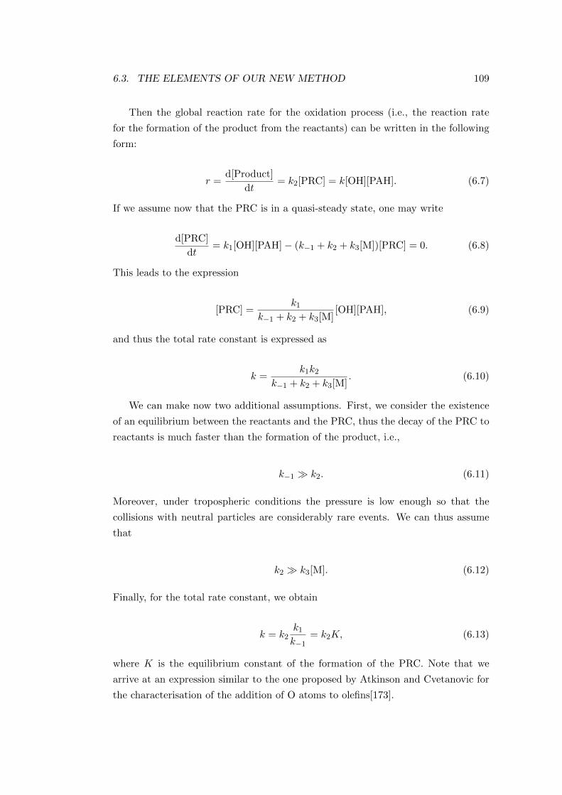
6.3. THE ELEMENTS OF OUR NEW METHOD 109
Then the global reaction rate for the oxidation process (i.e., the reaction rate
for the formation of the product from the reactants) can be written in the following
form:
r =d[Product]
dt= k2[PRC] = k[OH][PAH]. (6.7)
If we assume now that the PRC is in a quasi-steady state, one may write
d[PRC]
dt= k1[OH][PAH]− (k−1 + k2 + k3[M])[PRC] = 0. (6.8)
This leads to the expression
[PRC] =k1
k−1 + k2 + k3[M][OH][PAH], (6.9)
and thus the total rate constant is expressed as
k =k1k2
k−1 + k2 + k3[M]. (6.10)
We can make now two additional assumptions. First, we consider the existence
of an equilibrium between the reactants and the PRC, thus the decay of the PRC to
reactants is much faster than the formation of the product, i.e.,
k−1 k2. (6.11)
Moreover, under tropospheric conditions the pressure is low enough so that the
collisions with neutral particles are considerably rare events. We can thus assume
that
k2 k3[M]. (6.12)
Finally, for the total rate constant, we obtain
k = k2k1
k−1= k2K, (6.13)
where K is the equilibrium constant of the formation of the PRC. Note that we
arrive at an expression similar to the one proposed by Atkinson and Cvetanovic for
the characterisation of the addition of O atoms to olefins[173].
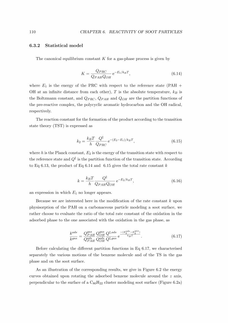
110 CHAPTER 6. REACTIVITY OF SOOT PARTICLES
6.3.2 Statistical model
The canonical equilibrium constant K for a gas-phase process is given by
K =QPRC
QPAHQOHe−E1/kBT , (6.14)
where E1 is the energy of the PRC with respect to the reference state (PAH +
OH at an infinite distance from each other), T is the absolute temperature, kB is
the Boltzmann constant, and QPRC , QPAH and QOH are the partition functions of
the pre-reactive complex, the polycyclic aromatic hydrocarbon and the OH radical,
respectively.
The reaction constant for the formation of the product according to the transition
state theory (TST) is expressed as
k2 =kBT
h
Q‡
QPRCe−(E2−E1)/kBT , (6.15)
where h is the Planck constant, E2 is the energy of the transition state with respect to
the reference state and Q‡ is the partition function of the transition state. According
to Eq 6.13, the product of Eq 6.14 and 6.15 gives the total rate constant k
k =kBT
h
Q‡
QPAHQOHe−E2/kBT , (6.16)
an expression in which E1 no longer appears.
Because we are interested here in the modification of the rate constant k upon
physisorption of the PAH on a carbonaceous particle modeling a soot surface, we
rather choose to evaluate the ratio of the total rate constant of the oxidation in the
adsorbed phase to the one associated with the oxidation in the gas phase, as
kads
kgas=QgasPAH
QadsPAH
QgasOH
QadsOH
Q‡,ads
Q‡,gase
−(Eads2 −Egas2
)
kBT . (6.17)
Before calculating the different partition functions in Eq 6.17, we characterised
separately the various motions of the benzene molecule and of the TS in the gas
phase and on the soot surface.
As an illustration of the corresponding results, we give in Figure 6.2 the energy
curves obtained upon rotating the adsorbed benzene molecule around the z axis,
perpendicular to the surface of a C80H22 cluster modeling soot surface (Figure 6.2a)
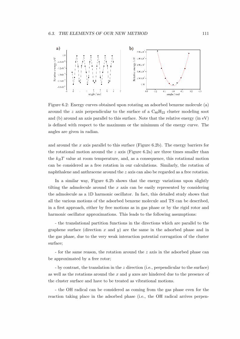
6.3. THE ELEMENTS OF OUR NEW METHOD 111
Figure 6.2: Energy curves obtained upon rotating an adsorbed benzene molecule (a)
around the z axis perpendicular to the surface of a C80H22 cluster modeling soot
and (b) around an axis parallel to this surface. Note that the relative energy (in eV)
is defined with respect to the maximum or the minimum of the energy curve. The
angles are given in radian.
and around the x axis parallel to this surface (Figure 6.2b). The energy barriers for
the rotational motion around the z axis (Figure 6.2a) are three times smaller than
the kBT value at room temperature, and, as a consequence, this rotational motion
can be considered as a free rotation in our calculations. Similarly, the rotation of
naphthalene and anthracene around the z axis can also be regarded as a free rotation.
In a similar way, Figure 6.2b shows that the energy variations upon slightly
tilting the admolecule around the x axis can be easily represented by considering
the admolecule as a 1D harmonic oscillator. In fact, this detailed study shows that
all the various motions of the adsorbed benzene molecule and TS can be described,
in a first approach, either by free motions as in gas phase or by the rigid rotor and
harmonic oscillator approximations. This leads to the following assumptions:
- the translational partition functions in the directions which are parallel to the
graphene surface (direction x and y) are the same in the adsorbed phase and in
the gas phase, due to the very weak interaction potential corrugation of the cluster
surface;
- for the same reason, the rotation around the z axis in the adsorbed phase can
be approximated by a free rotor;
- by contrast, the translation in the z direction (i.e., perpendicular to the surface)
as well as the rotations around the x and y axes are hindered due to the presence of
the cluster surface and have to be treated as vibrational motions.
- the OH radical can be considered as coming from the gas phase even for the
reaction taking place in the adsorbed phase (i.e., the OH radical arrives perpen-
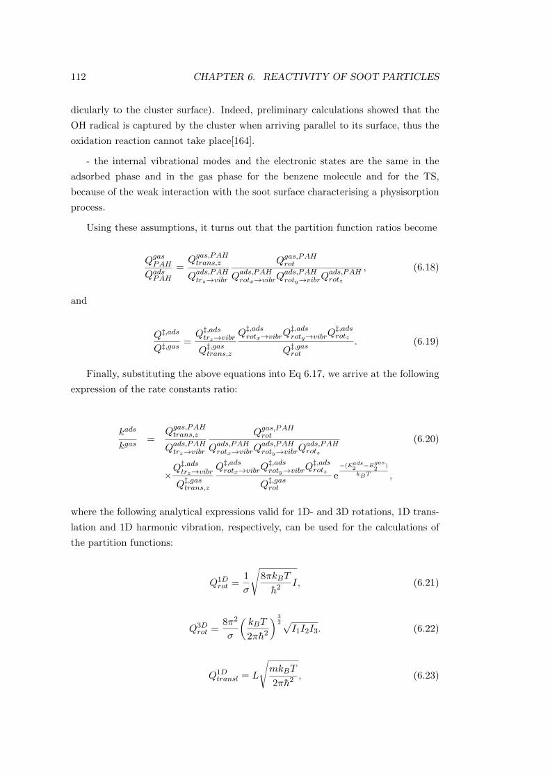
112 CHAPTER 6. REACTIVITY OF SOOT PARTICLES
dicularly to the cluster surface). Indeed, preliminary calculations showed that the
OH radical is captured by the cluster when arriving parallel to its surface, thus the
oxidation reaction cannot take place[164].
- the internal vibrational modes and the electronic states are the same in the
adsorbed phase and in the gas phase for the benzene molecule and for the TS,
because of the weak interaction with the soot surface characterising a physisorption
process.
Using these assumptions, it turns out that the partition function ratios become
QgasPAH
QadsPAH
=Qgas,PAHtrans,z
Qads,PAHtrz→vibr
Qgas,PAHrot
Qads,PAHrotx→vibrQads,PAHroty→vibrQ
ads,PAHrotz
, (6.18)
and
Q‡,ads
Q‡,gas=Q‡,adstrz→vibr
Q‡,gastrans,z
Q‡,adsrotx→vibrQ‡,adsroty→vibrQ
‡,adsrotz
Q‡,gasrot
. (6.19)
Finally, substituting the above equations into Eq 6.17, we arrive at the following
expression of the rate constants ratio:
kads
kgas=
Qgas,PAHtrans,z
Qads,PAHtrz→vibr
Qgas,PAHrot
Qads,PAHrotx→vibrQads,PAHroty→vibrQ
ads,PAHrotz
(6.20)
×Q‡,adstrz→vibr
Q‡,gastrans,z
Q‡,adsrotx→vibrQ‡,adsroty→vibrQ
‡,adsrotz
Q‡,gasrot
e−(Eads2 −Egas
2)
kBT ,
where the following analytical expressions valid for 1D- and 3D rotations, 1D trans-
lation and 1D harmonic vibration, respectively, can be used for the calculations of
the partition functions:
Q1Drot =
1
σ
√8πkBT
h2 I, (6.21)
Q3Drot =
8π2
σ
(kBT
2πh2
) 32√
I1I2I3. (6.22)
Q1Dtransl = L
√mkBT
2πh2 , (6.23)
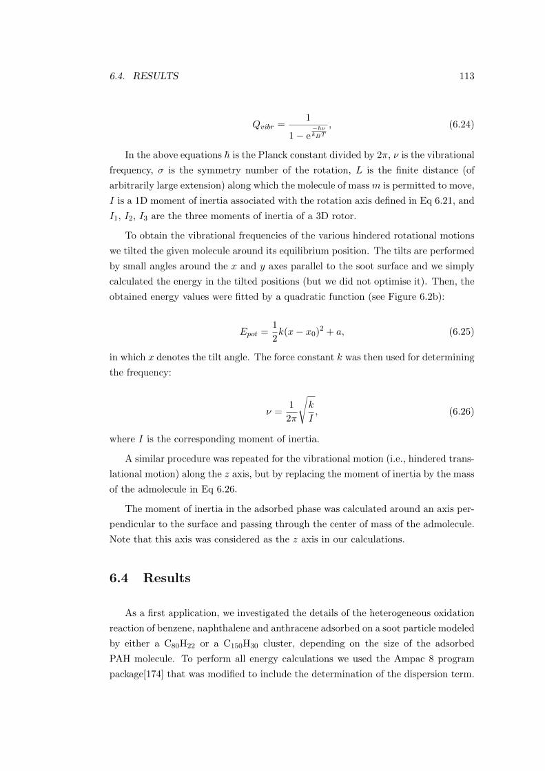
6.4. RESULTS 113
Qvibr =1
1− e−hνkBT
, (6.24)
In the above equations h is the Planck constant divided by 2π, ν is the vibrational
frequency, σ is the symmetry number of the rotation, L is the finite distance (of
arbitrarily large extension) along which the molecule of mass m is permitted to move,
I is a 1D moment of inertia associated with the rotation axis defined in Eq 6.21, and
I1, I2, I3 are the three moments of inertia of a 3D rotor.
To obtain the vibrational frequencies of the various hindered rotational motions
we tilted the given molecule around its equilibrium position. The tilts are performed
by small angles around the x and y axes parallel to the soot surface and we simply
calculated the energy in the tilted positions (but we did not optimise it). Then, the
obtained energy values were fitted by a quadratic function (see Figure 6.2b):
Epot =1
2k(x− x0)2 + a, (6.25)
in which x denotes the tilt angle. The force constant k was then used for determining
the frequency:
ν =1
2π
√k
I, (6.26)
where I is the corresponding moment of inertia.
A similar procedure was repeated for the vibrational motion (i.e., hindered trans-
lational motion) along the z axis, but by replacing the moment of inertia by the mass
of the admolecule in Eq 6.26.
The moment of inertia in the adsorbed phase was calculated around an axis per-
pendicular to the surface and passing through the center of mass of the admolecule.
Note that this axis was considered as the z axis in our calculations.
6.4 Results
As a first application, we investigated the details of the heterogeneous oxidation
reaction of benzene, naphthalene and anthracene adsorbed on a soot particle modeled
by either a C80H22 or a C150H30 cluster, depending on the size of the adsorbed
PAH molecule. To perform all energy calculations we used the Ampac 8 program
package[174] that was modified to include the determination of the dispersion term.
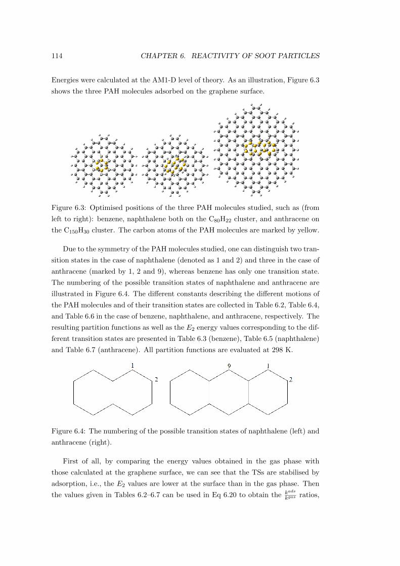
114 CHAPTER 6. REACTIVITY OF SOOT PARTICLES
Energies were calculated at the AM1-D level of theory. As an illustration, Figure 6.3
shows the three PAH molecules adsorbed on the graphene surface.
Figure 6.3: Optimised positions of the three PAH molecules studied, such as (from
left to right): benzene, naphthalene both on the C80H22 cluster, and anthracene on
the C150H30 cluster. The carbon atoms of the PAH molecules are marked by yellow.
Due to the symmetry of the PAH molecules studied, one can distinguish two tran-
sition states in the case of naphthalene (denoted as 1 and 2) and three in the case of
anthracene (marked by 1, 2 and 9), whereas benzene has only one transition state.
The numbering of the possible transition states of naphthalene and anthracene are
illustrated in Figure 6.4. The different constants describing the different motions of
the PAH molecules and of their transition states are collected in Table 6.2, Table 6.4,
and Table 6.6 in the case of benzene, naphthalene, and anthracene, respectively. The
resulting partition functions as well as the E2 energy values corresponding to the dif-
ferent transition states are presented in Table 6.3 (benzene), Table 6.5 (naphthalene)
and Table 6.7 (anthracene). All partition functions are evaluated at 298 K.
Figure 6.4: The numbering of the possible transition states of naphthalene (left) and
anthracene (right).
First of all, by comparing the energy values obtained in the gas phase with
those calculated at the graphene surface, we can see that the TSs are stabilised by
adsorption, i.e., the E2 values are lower at the surface than in the gas phase. Then
the values given in Tables 6.2–6.7 can be used in Eq 6.20 to obtain the kads
kgas ratios,
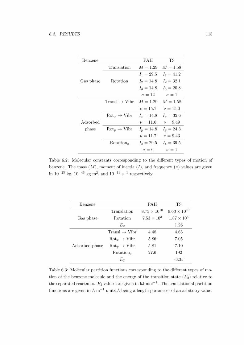
6.4. RESULTS 115
Benzene PAH TS
Translation M = 1.29 M = 1.58
I1 = 29.5 I1 = 41.2
Gas phase Rotation I2 = 14.8 I2 = 32.1
I3 = 14.8 I3 = 20.8
σ = 12 σ = 1
Transl → Vibr M = 1.29 M = 1.58
ν = 15.7 ν = 15.0
Rotx → Vibr Ix = 14.8 Ix = 32.6
Adsorbed ν = 11.6 ν = 9.49
phase Roty → Vibr Iy = 14.8 Iy = 24.3
ν = 11.7 ν = 9.43
Rotationz Iz = 29.5 Iz = 39.5
σ = 6 σ = 1
Table 6.2: Molecular constants corresponding to the different types of motion of
benzene. The mass (M), moment of inertia (I), and frequency (ν) values are given
in 10−25 kg, 10−46 kg m2, and 10−11 s−1 respectively.
Benzene PAH TS
Translation 8.73× 10¹⁰ 9.63× 10¹⁰
Gas phase Rotation 7.53× 10³ 1.87× 10⁵
E2 1.26
Transl → Vibr 4.48 4.65
Rotx → Vibr 5.86 7.05
Adsorbed phase Roty → Vibr 5.81 7.10
Rotationz 27.6 192
E2 -3.35
Table 6.3: Molecular partition functions corresponding to the different types of mo-
tion of the benzene molecule and the energy of the transition state (E2) relative to
the separated reactants. E2 values are given in kJ mol−1. The translational partition
functions are given in L m−1 units L being a length parameter of an arbitrary value.
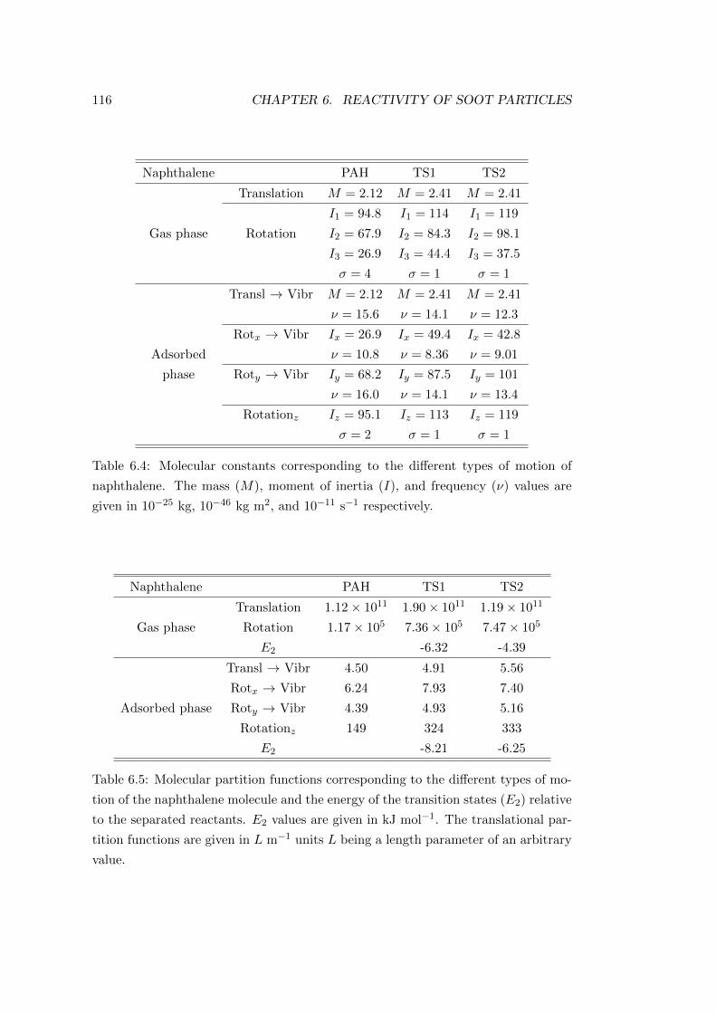
116 CHAPTER 6. REACTIVITY OF SOOT PARTICLES
Naphthalene PAH TS1 TS2
Translation M = 2.12 M = 2.41 M = 2.41
I1 = 94.8 I1 = 114 I1 = 119
Gas phase Rotation I2 = 67.9 I2 = 84.3 I2 = 98.1
I3 = 26.9 I3 = 44.4 I3 = 37.5
σ = 4 σ = 1 σ = 1
Transl → Vibr M = 2.12 M = 2.41 M = 2.41
ν = 15.6 ν = 14.1 ν = 12.3
Rotx → Vibr Ix = 26.9 Ix = 49.4 Ix = 42.8
Adsorbed ν = 10.8 ν = 8.36 ν = 9.01
phase Roty → Vibr Iy = 68.2 Iy = 87.5 Iy = 101
ν = 16.0 ν = 14.1 ν = 13.4
Rotationz Iz = 95.1 Iz = 113 Iz = 119
σ = 2 σ = 1 σ = 1
Table 6.4: Molecular constants corresponding to the different types of motion of
naphthalene. The mass (M), moment of inertia (I), and frequency (ν) values are
given in 10−25 kg, 10−46 kg m2, and 10−11 s−1 respectively.
Naphthalene PAH TS1 TS2
Translation 1.12× 10¹¹ 1.90× 10¹¹ 1.19× 10¹¹
Gas phase Rotation 1.17× 10⁵ 7.36× 10⁵ 7.47× 10⁵
E2 -6.32 -4.39
Transl → Vibr 4.50 4.91 5.56
Rotx → Vibr 6.24 7.93 7.40
Adsorbed phase Roty → Vibr 4.39 4.93 5.16
Rotationz 149 324 333
E2 -8.21 -6.25
Table 6.5: Molecular partition functions corresponding to the different types of mo-
tion of the naphthalene molecule and the energy of the transition states (E2) relative
to the separated reactants. E2 values are given in kJ mol−1. The translational par-
tition functions are given in L m−1 units L being a length parameter of an arbitrary
value.
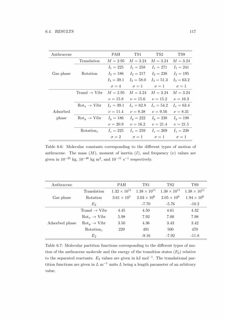
6.4. RESULTS 117
Anthracene PAH TS1 TS2 TS9
Translation M = 2.95 M = 3.24 M = 3.24 M = 3.24
I1 = 225 I1 = 258 I1 = 271 I1 = 241
Gas phase Rotation I2 = 186 I2 = 217 I2 = 238 I2 = 195
I3 = 39.1 I3 = 58.0 I3 = 51.3 I3 = 63.2
σ = 4 σ = 1 σ = 1 σ = 1
Transl → Vibr M = 2.95 M = 3.24 M = 3.24 M = 3.24
ν = 15.8 ν = 15.6 ν = 15.2 ν = 16.3
Rotx → Vibr Ix = 39.1 Ix = 62.8 Ix = 54.2 Ix = 63.4
Adsorbed ν = 11.4 ν = 8.38 ν = 9.56 ν = 8.31
phase Roty → Vibr Iy = 186 Iy = 222 Iy = 238 Iy = 198
ν = 20.9 ν = 16.2 ν = 21.4 ν = 21.5
Rotationz Iz = 225 Iz = 259 Iz = 269 Iz = 238
σ = 2 σ = 1 σ = 1 σ = 1
Table 6.6: Molecular constants corresponding to the different types of motion of
anthracene. The mass (M), moment of inertia (I), and frequency (ν) values are
given in 10−25 kg, 10−46 kg m2, and 10−11 s−1 respectively.
Anthracene PAH TS1 TS2 TS9
Translation 1.32× 10¹¹ 1.38× 10¹¹ 1.38× 10¹¹ 1.38× 10¹¹
Gas phase Rotation 3.61× 10⁵ 2.03× 10⁶ 2.05× 10⁶ 1.94× 10⁶
E2 -7.70 -5.76 -10.2
Transl → Vibr 4.45 4.50 4.61 4.32
Rotx → Vibr 5.98 7.92 7.00 7.98
Adsorbed phase Roty → Vibr 3.50 4.36 3.43 3.42
Rotationz 229 491 500 470
E2 -9.16 -7.92 -11.8
Table 6.7: Molecular partition functions corresponding to the different types of mo-
tion of the anthracene molecule and the energy of the transition states (E2) relative
to the separated reactants. E2 values are given in kJ mol−1. The translational par-
tition functions are given in L m−1 units L being a length parameter of an arbitrary
value.
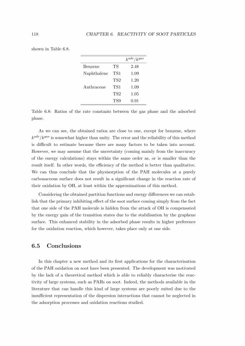
118 CHAPTER 6. REACTIVITY OF SOOT PARTICLES
shown in Table 6.8.
kads/kgas
Benzene TS 2.48
Naphthalene TS1 1.09
TS2 1.20
Anthracene TS1 1.09
TS2 1.05
TS9 0.91
Table 6.8: Ratios of the rate constants between the gas phase and the adsorbed
phase.
As we can see, the obtained ratios are close to one, except for benzene, where
kads/kgas is somewhat higher than unity. The error and the reliability of this method
is difficult to estimate because there are many factors to be taken into account.
However, we may assume that the uncertainty (coming mainly from the inaccuracy
of the energy calculations) stays within the same order as, or is smaller than the
result itself. In other words, the efficiency of the method is better than qualitative.
We can thus conclude that the physisorption of the PAH molecules at a purely
carbonaceous surface does not result in a significant change in the reaction rate of
their oxidation by OH, at least within the approximations of this method.
Considering the obtained partition functions and energy differences we can estab-
lish that the primary inhibiting effect of the soot surface coming simply from the fact
that one side of the PAH molecule is hidden from the attack of OH is compensated
by the energy gain of the transition states due to the stabilisation by the graphene
surface. This enhanced stability in the adsorbed phase results in higher preference
for the oxidation reaction, which however, takes place only at one side.
6.5 Conclusions
In this chapter a new method and its first applications for the characterisation
of the PAH oxidation on soot have been presented. The development was motivated
by the lack of a theoretical method which is able to reliably characterise the reac-
tivity of large systems, such as PAHs on soot. Indeed, the methods available in the
literature that can handle this kind of large systems are poorly suited due to the
insufficient representation of the dispersion interactions that cannot be neglected in
the adsorption processes and oxidation reactions studied.
6.5. CONCLUSIONS 119
To calculate the interaction energies, the SE-D method was thus used because
it was proved to properly describe the interactions between large aromatic systems,
and therefore it can be used to study systems for which full ab initio calculations
are prohibited because of their large size.
In our calculations the soot particle was modeled by a large, flat, defect-free,
graphene-like surface. Our results have shown that the physisorption of the PAH
molecules at the soot surface does not change dramatically the reaction rate of the
oxidation of PAHs by OH as compared to that occurring in the gas phase. It should
be noted that a real surface may contain chemical defects that can lead to the
modification of these results to an unknown extent. It should also be noted that the
rate constants in the adsorbed phase may depend on the coverage of the soot surface.
Moreover, the aforementioned capture of the OH radical by the surface can also lead
to different conclusions because this should decrease the efficiency of the oxidation
reaction at the surface. Finally, the aggregation or possible multilayer adsorption
of the PAH molecules makes also more difficult the comparison of the experimental
results with those obtained from the theory.
Nevertheless, the SE-D method represents a real improvement with respect to
other quantum chemical methods because it can be used for characterising very large
systems with relatively low computational costs. Furthermore, it can easily be used
to take into account finite coverages, and it can also be reparametrised to include
surface defects. Finally, it should be mentioned that the application of this method
can be extended to other carbonaceous systems, such as nanotubes and fullerenes.
Chapter 7
Conclusions and perspectives
In this thesis, I have presented a series of theoretical studies aiming at charac-
terising, at a molecular level, the adsorption of various compounds on the surface
of solid particles present in the Earth’s atmosphere. The corresponding numerical
studies were devoted to ice and soot particles which are abundant in the atmosphere
and which represent a major source of uncertainties in the current climate models.
The results presented here clearly show that atmospheric science may profit by
the use of theoretical methods. As a matter of fact, experimental research will never
be able to produce such an insight into the investigated phenomena that simulation
techniques and other theoretical methods do. Making models and predictions will
always be indispensable to obtain a complete picture of the examined processes. By
contrast, theoretical work is worth nothing without experiences, and it must always
be carried out and interpreted in light of the knowledge based on experimental data.
Doubtlessly, these two aspects fruitfully supporting and complementing each other
must be combined to achieve a more fundamental understanding of the phenomena
of our world.
My thesis has been based on three main subjects. The first has been devoted
to the study of the adsorption of acetone, formic acid and benzaldehyde on the
surface of ice. When carrying out adsorption measurements, owing to technical limi-
tations one has to face several restrictions which result in limited accuracy and range
of examination. The use of the GCMC method has not only provided adsorption
isotherms in the whole pressure range but also revealed the mechanism of the ad-
sorption processes by identifying the preferred orientations of the admolecules and
the corresponding interaction energies. Moreover, the fundamental role of hydrogen
bonding between the adsorbed molecules and the ice surface has been evidenced,
120
121
as well as the increasing importance of the lateral interactions when increasing the
pressure. Above a certain pressure, these lateral interactions become finally the
main driving force of the adsorption which cannot be neglected in the interpretation
of the experimental data. The comparison of the results of these studies with the
experimental data has been excellent, which, on one hand, confirms the suitability
of the used potential models to describe the systems investigated, and, on the other
hand, stresses again the importance of simulation techniques in the study of hardly
observable processes. Further research should be directed toward the competitive
adsorption of different volatile organic compounds as they are present jointly in the
atmosphere, and to the role of defects (such as ions) in the adsorption processes at
the ice surface.
My second subject is concerned with the role of the characteristics of soot par-
ticles that might affect ice nucleation at their surface. For this purpose, water
adsorption on various particles containing, on one hand, cavities of different shape
and, on the other hand, carbon atoms of different numbers have been investigated.
The results have shown that the size and the shape of pores are of special interest:
The more spherical the cavity is, the more effective the adsorption can be. The pres-
ence of oxidised functional groups inside the cavity does not change the maximum
number of water molecules that may be trapped in it, but it enhances the affinity
of water molecules for the soot at low pressure. This results in the appearance of
the adsorbates in the cavity at significantly lower pressure as compared to the bare
carbonaceous particle. In the future, the adsorption of water on a non-rigid soot
particle, i.e., that can be deformed during the adsorption process should be studied.
Understanding the formation of soot particles at high temperatures could also be of
great interest.
The last topic of this thesis is related to the reactivity of soot particles in the
atmosphere. A new model has been presented to compare the oxidation reaction of
PAH molecules by the OH radical in the gas phase with that taking place when the
PAH molecules are adsorbed on a perfect carbonaceous surface. The soot–PAH inter-
action as well as the PAH–OH interaction have been described by the SE-D method,
which provides an appropriate energetic characterisation of large carbonaceous sys-
tems. The detailed analysis of the reactions taking place in the different phases has
revealed that the primary inhibiting effect of the soot surface (namely that it hides
one side of the PAH molecule from the OH attack) is compensated by the energy
gain of the transition state of the oxidation reaction. The joint quenching of these
two effects results in a similar reaction rate of oxidation of PAHs by OH in the gas
phase and in the adsorbed phase at a perfect carbonaceous surface. This research

122 CHAPTER 7. CONCLUSIONS AND PERSPECTIVES
might be extended to the study of structurally and chemically defected surfaces, and
to the impact of varying surface coverage of PAH molecules on the reaction rate of
the oxidation. It should be mentioned that the accuracy of the theoretical results
obtained here (i.e., the accuracy of the parameters of the SE-D method) could only
be checked by comparison with experimental results on well-defined carbonaceous
systems which are unfortunately largely missing up to now. Finally, it is also worth
noting that the SE-D method could be extended to reactions taking place at other
carbonaceous surfaces such as graphene, fullerene, or nanotubes.
Bibliography
[1] R.P. Wayne. Chemistry of Atmospheres. (3rd Edition, OUP, 2000)
[2] D.J. Jacob. Introduction to Atmospheric Chemistry. (Princeton University
Press, 1999)
[3] G.P. Brasseur, J.J. Orlando and G.S. Tyndall. Atmospheric Chemistry and
Global Change. (OUP, 1999)
[4] J.H. Seinfeld and S.N. Pandis. Atmospheric Chemistry and Physics : From
Air Pollution to Climate Change. (Wiley, 1998)
[5] S.M. Saunders, M.E. Jenkin, R.G. Derwent, and M. J. Pilling. Atmos. Chem.
Phys., 3 (2003) 161.
[6] M.E. Jenkin, S.M. Saunders, V. Wagner, and M. J. Pilling. Atmos. Chem.
Phys., 3 (2003) 181.
[7] R.G. Derwent, M.E. Jenkin, and S.M. Saunders. Atmos. Environ., 30 (1996)
181.
[8] http://mcm.leeds.ac.uk/MCM/
[9] R.C. Pierce and M. Katz. Environ. Sci. Technol., 9 (1975) 347.
[10] U.Poschl, T. Letzel, C. Schauer, and R. Niessner. J. Phys. Chem. A, 105
(2001) 4029.
[11] D.G. Aubin, J.P.D. Abbatt. Environ. Sci. Technol., 40 (2006) 179.
[12] R. Kotzick, U. Panne, and R. Niessner. J. Aerosol. Sci., 28 (1997) 725.
[13] T. Novakov and C.E. Corrigan. Geophys. Res. Lett., 23 (1996) 2141.
[14] C.N. Cruz and S.N. Pandis. Atmos. Environ., 31 (1997) 2205.
123
124 BIBLIOGRAPHY
[15] G.T. Wolf and R.L. Klimisch, Eds. Particulate Carbon, atmospheric life cycle.
(Plenum Press: New York, 1982.)
[16] D.K. Lynch, K. Sassen, D.O. Starr, G. Stephens. Cirrus. (OUP, New York,
2002).
[17] S. Solomon, S. Borrmann, R.R. Garcia et al. J. Geophys. Res., 102 (1997)
21411.
[18] P. Konopka and W. Vogelsberger. J. Geophys. Res., 102 (1997) 16057.
[19] U. Schumann, J. Strom, R. Busen, R. Baumann, K. Gierens, M. Krautstrunk,
F.P. Schroder, J. Stingl. J. Geophys. Res., 101 (1996) 6853.
[20] V. Williams et R.B. Noland. Transport. Res. Part D, 10 (2005) 269.
[21] J. Penner, D. Lister, D. Griggs, D. Dokken, and M. McFarland. IPCC Special
Report, Aviation and the global atmosphere. (Cambridge University Press,
1999).
[22] P. Forster, V. Ramaswamy, P. Artaxo, T. Berntsen, R. Betts, D. Fahey, J.
Haywood, J. Lean, D. Lowe, G. Myhre, et al., Fourth Assessment Report
of the Intergovernmental Panel on Climate Change, Climate Change 2007 :
The Physical Science Basis. (Cambridge University Press, Cambridge, United
Kingdom and New York, NY, USA., 2007).
[23] C.S. Zerefos, K. Eleftheratos, D.S. Balis, P. Zanis, G. Tselioudis. Atmos.
Chem. Phys., 3 (2003) 1633.
[24] O. Boucher. Nature. 397 (1999) 30.
[25] B. Karcher, M. Hirschberg, and P. Fabian. Journal of Geophysical Research
D: Atmospheres, 101 15169 (1996) 15169 .
[26] G. Gleitsmann and R. Zellne. Atm. Envir., 32 (1998) 3079.
[27] C. Sergides, J. Jassim, A. Chughtai, and D. Smith. Appl. Spectr., 41 (1987)
482.
[28] D. Smith, W. Welch, J. Jassim, A. Chughtai, and D. Stedman. Appl. Spectr.,
42 (1988) 1473.
[29] B. Karcher. Atmospheric Research, 46 (1998) 293.
BIBLIOGRAPHY 125
[30] P. DeMott, Y. Chen, S. Kreidenweis, D. Rogers, and D. Sherman. Geophys.
Res. Lett., 26 (1999) 2429.
[31] C. Alcala-Jornod, H. van den Bergh, and M. Rossi. Geophys. Res. Lett., 29
(2002) 1.
[32] D. Ferry, J. Suzanne, S. Nitsche, O.B. Popovcheva, N.K. Shonija. J. Geophys.
Res., 107 (2002) 4734.
[33] G. J. Young, J. J. Chessick, F. H. Healey, and A. C. Zettlemoyer. J. Chem.
Phys., 58 (1954) 313.
[34] M. M. Dubinin. Carbon, 18 (1980) 355.
[35] O. Popovicheva and A. Starik. Izvestiya - Atmospheric and Ocean Physics,
43 (2007) 125.
[36] H. Richter and J.B. Howard. Progress in Energy Combustion Science, 26
(2000) 565.
[37] I.M. Kennedy. Progr. Energy Combust. Sci., 23 (1997) 95.
[38] O. Popovicheva, A. Starik, and O. Favorskii. Izv. Akad. Nauk, Fiz. Atmos.
Okeana, 36 (2000) 163.
[39] R. Dhaubhadel, F. Pierce, A. Chakrabarti, C.M. Sorensen. Phys. Rev. E, 73
(2006) 011404.
[40] O. Popovicheva, N. Persiantseva, B. Kuznetsov, T. Rakhmanova, N. Shonija,
J. Suzanne, and D. Ferry. J. Phys. Chem. A, 107 (2003) 10046.
[41] B. Demirdjian, D. Ferry, J. Suzanne, O. B. Popovicheva, N. M. Persiantseva,
and N. K. Shonija. J. Atm. Chem., 56 (2007) 83.
[42] M.P. Allen, D.J. Tildesley. Computer Simulation of Liquids. (OUP, Oxford,
1987)
[43] N. Metropolis, A.W. Rosenbluth, M.N. Rosenbluth, A.H. Teller, and E. Teller.
J. Chem. Phys., 21 (1953) 1087.
[44] G.E. Norman, V.S. Filinov. High Temp USSR, 7, 216 (1969) 216.
[45] D. J. Adams. Mol. Phys., 28 (1974) 1241.
[46] D. J. Adams. Mol. Phys., 29 (1975) 307.
126 BIBLIOGRAPHY
[47] M. Mezei. Mol. Phys., 40 (1980) 901.
[48] M. Mezei. Mol. Phys., 61 (1987) 565. Erratum: Mol. Phys. 67 (1989) 1207.
[49] L. Verlet. Phys. Rev., 159 (1967) 98.
[50] A.J. Stone. The theory of intermolecular forces. (Oxford University Press,
1997)
[51] A. Warshel, R.M. Weiss. JACS, 102 (1980) 6218.
[52] D.W.M. Hofmann, L. N. Kuleshova, B. D’Aguanno. Chem. Phys. Lett., 448
(2007) 138.
[53] van Duin, Dasgupta, Lorant, Goddard. J. phys. chem. A, 105 (2001) 9396.
[54] D.W. Brenner. Phys. Rev. B, 42 (1990) 9458.
[55] G.C Abell. Phys. Rev. B, 31 (1985) 6184.
[56] J. Tersoff. Phys. Rev. Lett. 56 (1986) 632.
[57] S.J. Stuart, A.B. Tutein, J.A. Harrison. J. Chem. Phys., 112 (2000) 6472.
[58] J.A. Barker, R.O. Watts. Mol. Phys., 26 (1973) 789.
[59] M. Neumann. J. Chem. Phys., 82 (1985) 563.
[60] S. Nose and M.L. Klein. Mol. Phys., 50, (1983) 1055.
[61] P.P. Ewald. Ann. Phys., 21 (1921) 1087.
[62] M.J.S. Dewar, E.G. Zoebisch, E.F. Healy and J.J.P. Stewart. JACS, 107
(1985) 3902.
[63] M.J.S. Dewar and W. Thiel. JACS, 99 (1977) 4899.
[64] J.J.P. Stewart. J. Comput. Chem., 10 (1989) 209.
[65] F. Domine and L. Rey-Hanot. Geophys. Res. Lett., 29 (2002) 1873.
[66] C. Guimbaud, A. Grannas, P. Shepson, J. Fuentes, H. Boudries, J. Botten-
Heim, F. Domine, S. Houdier, S. Perrier, T. Biesenthal and B. Splawn. Atmos.
Environ., 36 (2002) 2743.
[67] T. Bartels-Rausch, C. Guimbaud, H. W. Gaggeler and M. Ammann. Geophys.
Res. Lett., 31 (2004) L16110.
BIBLIOGRAPHY 127
[68] P. K. Hudson,M. A. Zondlo and M.A. Tolbert. J. Phys. Chem. A, 106 (2002)
2882.
[69] N. Peybernes, C. Marchand, S. Le Calve and P. Mirabel. Phys. Chem. Chem.
Phys., 6 (2004) 1277.
[70] P. Behr, A. Terziyski and R. Zellner. J. Phys. Chem. A, 110 (2006) 8098.
[71] D.J. Donaldson and D. Anderson. J. Phys. Chem. A, 103 (1999) 871.
[72] A.K. Winkler, N.S. Holmes and J.N. Crowley. Phys. Chem. Chem. Phys., 4
(2002) 5270.
[73] O. Sokolov and J.P.D. Abbatt. J. Phys. Chem. A, 106 (2002) 775.
[74] P. von Hessberg, N. Pouvesle, A.K. Winkler, G. Schuster and J.N. Crowley,
Phys. Chem. Chem. Phys., 10 (2008) 2345.
[75] P. Jedlovszky, G. Hantal, K.Neurohr, S. Picaud, P.N.M. Hoang, P. von Hess-
berg and J.N. Crowley, J. Phys. Chem. C, 112 (2008) 8976.
[76] P. Jedlovszky, L. Partay, P.N.M. Hoang, S. Picaud, P. von Hessberg and J.N.
Crowley, J. Am. Chem. Soc., 128 (2006) 15300.
[77] F. Marinelli, A. Allouche. Chem. Phys., 272 (2001) 137.
[78] A. Allouche. J. Chem. Phys., 112 (2005) 234703.
[79] S. Bahr, A. Borodin, O. Hofft, V. Kempter, A. Allouche. J. Chem. Phys., 112
(2005) 234704.
[80] S. Picaud, P.N.M. Hoang, N. Peybernes, S Le Calve, P. Mirabel. J. Chem.
Phys., 122 (2005) 194707.
[81] S. Picaud, P.N.M. Hoang. J. Chem. Phys., 112 (2000) 9898.
[82] M. Compoint, C. Toubin, S. Picaud, P.N.M. Hoang, C. Girardet, Chem. Phys.
Lett., 365 (2002) 1.
[83] B. Collignon, S. Picaud. Chem. Phys. Lett., 393 (2004) 457.
[84] N. Peybernes, S. Le Calve, P. Mirabel, S. Picaud, P.N.M. Hoang. J.
Phys.Chem. B, 108 (2004) 17425.
[85] L.B. Partay, P. Jedlovszky, P.N.M. Hoang, S. Picaud, M. Mezei. J. Phys.
Chem. C, 111 (2007) 9407.
128 BIBLIOGRAPHY
[86] G. Hantal, P. Jedlovszky, P.N.M. Hoang, S. Picaud. J. Phys. Chem. C, 111
(2007) 14170.
[87] L. Turi. J. Phys. Chem., 100 (1996) 11285.
[88] (a) P. Jedlovszky, L. Turi. J. Phys. Chem. B, 101 (1997) 5429. (b) Erratum:
P. Jedlovszky, L. Turi. J. Phys. Chem. B, 103 (1999) 3510.
[89] M. Mezei, MMC: Monte Carlo program for simulation of molecular assem-
blies, URL: http://inka.mssm.edu/mezei/mmc.
[90] C.D. Daub, G.N. Patey, D.B. Jack and A.K. Sallabi. J. Chem. Phys., 124
(2006) 114706.
[91] S. Brunauer, P.H. Emmett and E. Teller. J. Am. Chem. Soc., 60 (1938) 309.
[92] P. Jedlovszky, A. Vincze and G. Horvai. J. Chem. Phys., 117 (2002) 2271.
[93] P. Jedlovszky, A. Vincze and G. Horvai, Phys. Chem. Chem. Phys., 6 (2004)
1874.
[94] A. Perera and F. Sokolic. J. Chem. Phys., 121 (2004) 11272.
[95] A. Perera, F. Sokolic, L. Almasy, P. Westh and Y. Koga, J. Chem. Phys.,
123 (2005) 024503.
[96] M. Ferrario, M. Haughney, I.R. McDonald and M.L. Klein. J. Chem. Phys.,
93 (1990) 5156.
[97] W.L. Jorgensen, J.M. Briggs and M.L. Contreras, J. Phys. Chem., 94 (1990)
1683.
[98] P. Jedlovszky and G. Palinkas, Mol. Phys., 84 (1995) 217.
[99] J.M. Hermida-Ramon and M.A. Rıos. J. Phys. Chem. A, 102(1998) 2594.
[100] S. Weerasinghe and P.E. Smith. J. Chem. Phys., 118 (2003) 10663.
[101] H.J.C. Berendsen, J.R. Grigera and T.P. Straatsma. J. Phys. Chem., 91
(1987) 6269.
[102] P.P. Ewald, Ann. Phys., 21, 21, 1087.
[103] M. Riikonen, M. Sillanpaa, L. Virta, D. Sullivan, J. Moilanen and I. Luukko-
nen. Appl. Opt., 39 (2000) 6080.
BIBLIOGRAPHY 129
[104] J. Goodman, O.B. Toon, R.F. Pueschel, K.G. Snetsinger and S.J. Verma. J.
Geophys. Res., 94 (1989) 16449.
[105] J.E. Schaff and J.T. Roberts. J. Phys. Chem., 100 (1996) 14151.
[106] J.E. Schaff and J.T. Roberts. Langmuir, 14 (1998) 1478.
[107] P. Behr, U. Scharfenort, A. Terziyski, K. Demiral and R. Zellner. in Com-
bustion and Atmospheric Pollution, International Symposium on Atmospheric
Pollution, ed. G. D. Ray, S. M. Forlov and A. M. Starik, Torus Press, Moscow,
2003, pp. 575578.
[108] L. Partay, P. Jedlovszky and G. Horvai, J. Phys. Chem. B, 109 (2005) 12014.
[109] S. Mitlin and K. T. Leung. Surf. Sci., 505 (2002) L227.
[110] F. Marinelli and A. Allouche. Chem. Phys., 272 (2001) 137.
[111] (a) P. Jedlovszky, L. Turi. J. Phys. Chem. A, 101 (1997) 2662. (b) Erratum:
P. Jedlovszky, L. Turi. J. Phys. Chem. A, 103 (1999) 3796.
[112] M. Mahoney, W.L. Jorgensen. J. Chem. Phys., 112 (2000) 8910.
[113] P. Jedlovszky, G. Hantal, K. Neurohr, S. Picaud, P.N.M. Hoang, .P von
Hessberg, J.N. Crowley. J. Phys. Chem. C, 112, (2008) 8976.
[114] NIST Standard Reference Database Number 69, NIST Chemistry Webbook
Edition, http://webbook.nist.gov/chemistry/. (2005).
[115] S. Bahr, V. Kempter. J. Phys. Chem. C 111 (2007) 11302.
[116] D. Wei, J.F. Truchon, S. Sirois, D. Salahub. J. Chem. Phys. 116 (2002) 6028.
[117] W.L. Jorgensen, D.S. Maxwell, J.J. Tirado-Rives. J. Am. Chem. Soc., 118
(1996) 11225.
[118] S. Canneaux, J.C. Soetens, E. Henon, F. Bohr. Chem. Phys., 237 (2006) 212.
[119] M. Petitjean, G. Hantal, C. Chauvin, Ph. Mirabel, S. Le Calve, P.N.M.
Hoang, S. Picaud, P. Jedlovszky Langmuir, DOI: 10.1021/1a100169h.
[120] R.K. Sinnot. Chemical Engineering Design, 4th ed. Coulson and Richardson’s
Chemical Engineering Series, Vol. 6; (Elsevier Butterworth-Heinemann: Ox-
ford, U.K., 2005.)
[121] S. Bahr, V. Kempter. J. Chem. Phys. 127 (2007) 074707.
130 BIBLIOGRAPHY
[122] O.B. Popovicheva, M.E. Trukhin, N.M. Persiantseva, and N.K. Shonija, At-
mosph. Environ., 35 (2001) 1673.
[123] E.A. Muller, L.F. Rull, L.F. Vega, and K.E. Gubbins. J. Phys. Chem., 100
(1996) 1189.
[124] E.A. Muller and K.E. Gubbins. Carbon, 36 (1998) 1433.
[125] C.L. McCallum, T.J. Bandosz, S.C. McGrother, E.A. Mller, and K.E. Gub-
bins. Langmuir, 15 (1999) 533.
[126] J.K. Brennan, T.J. Bandosz, K.T. Thomson, and K.E. Gubbins. Colloids
Surf., 187-188 (2001) 539.
[127] M.Jorge, C.Schumacher, and N.A. Seaton. Langmuir, 18 (2002) 9296.
[128] A.Striolo, A.A. Chialvo, K.E. Gubbins, and P.T. Cummings. J. Chem. Phys.,
122 (2005) 234712.
[129] S. Hamad, J.A. Mejias, S. Lago, S. Picaud, and P.N.M. Hoang. J. Phys.
Chem. B, 108 (2004) 5405.
[130] B. Collignon, P.N.M. Hoang, S.Picaud, and J.C. Rayez. Chem. Phys. Lett.,
406 (2005) 430.
[131] B.Collignon, P.N.M. Hoang, S.Picaud, and J.C. Rayez. Comp. Lett., 1 (2005)
277.
[132] M. Oubal, S.Picaud, M.T.Rayez, and J.C.Rayez. Carbon (2010) in press
(doi:10.1016/j.carbon.2009.12.054).
[133] S. Picaud, P.N.M. Hoang, S.Hamad, J.A. Mejias, and S. Lago. J. Phys. Chem.
B, 108 (2004) 5410.
[134] S. Picaud, B. Collignon, P.N.M. Hoang, and J.C. Rayez. J. Phys. Chem., 110
(2006) 8398.
[135] S. Picaud, B.Collignon, P.N.M. Hoang, and J.C. Rayez. Phys. Chem. Chem.
Phys., 10 (2008) 6998.
[136] F. Moulin, S. Picaud, P.N.M. Hoang, L. Partay, and P. Jedlovszky. Mol.
Simul., 32 (2006) 487.
[137] F. Moulin, S. Picaud, P.N.M. Hoang, and P. Jedlovszky. J. Chem. Phys., 127
(2007) 164719.
BIBLIOGRAPHY 131
[138] A.V. Shevade, S. Jiang, and K.E. Gubbins. Mol. Phys., 97 (1999) 1139.
[139] W.L. Jorgensen, J. Chandrasekhar, J.F. Madura, R.W. Impey, and M.L.
Klein, J. Chem. Phys., 79 (1983) 926.
[140] N.N. Medvedev, in Voronoi’s Impact on Modern Science, Vol. 1-2, edited by
P. Engel and H. Syta (Institute of Mathematics, Kiev, 1998), pp. 164-175.
[141] H. Edelsbrunner, M.A. Facello, and J.Liang. Discrete Appl. Math., 88 (1998)
83.
[142] M.G. Alinchenko, A.V. Anikeenko, N.N. Medvedev, V.P. Voloshin, M. Mezei,
and P. Jedlovszky. J. Phys. Chem. B, 108 (2004) 19056.
[143] M.G. Alinchenko, V.P. Voloshin, N.N. Medvedev, M. Mezei, L. Partay, and
P. Jedlovszky. J. Phys. Chem. B, 109 (2005) 16490.
[144] G. Malavasi, M.C. Menziani, A. Pedone, and U. Segre. J. Non-Cryst. Solids,
352 (2006) 285.
[145] G.F. Voronoi. J. Reine Angew. Math., 134 (1908) 198.
[146] B.N. Delaunay. Proc. Math. Congress in Toronto Aug.11-16 1924, 695 (1928).
[147] A. Okabe, B. Boots, K. Sugihara, and S.N. Chiu. Spatial Tessellations: Con-
cepts, and Applications of Voronoi Diagrams (Wiley, Chichester, 2000).
[148] N.N. Medvedev, The Voronoi-Delaunay Method in the Structural Investiga-
tion of Non-crystalline Systems (SB RAS: Novosibirsk, 2000), in Russian.
[149] See, for example, a geometric library at http://www.cgal.org/.
[150] N.N. Medvedev, V.P. Voloshin, V.A. Luchnikov, and M.L.Gavrilova, J. Comp.
Chem., 27 (2006) 1676.
[151] J. Dachs and S.J. Eisenreich. Environ. Sci. Technol., 34 (2000) 3690.
[152] R.L. Vander Wal, A.J. Tomasek. Combustion and Flame, 136 (2004) 129.
[153] J.M.E Storey and J.F. Pankow. Atmos. Environ. A, 26 (1992) 435.
[154] K.U. Goss and S.J. Eisenreich. Atmos. Environ., 31 (1997) 2827.
[155] B.T. Mader and J.F. Pankow. Environ. Sci. Technol., 36 (2002) 5218.
[156] B. Ngabe and L. Poissant. Environ. Sci. Technol., 37 (2003) 2094.
132 BIBLIOGRAPHY
[157] W. Esteve, H. Budzinski, and E. Villenave. Atmos. Environ., 38 (2004) 6063.
[158] N.K. Lee, S. Park, and S.L. Kim. J. Chem. Phys., 116 (2002) 7902.
[159] M.O. Sinnokrot, E.F. Valeev, and C.D. Sherrill. J. Am. Chem. Soc., 124
(2002) 10887.
[160] C. Gonzales, T.C. Allison, and E.C. Lim. J. Phys. Chem. A, 105 (2001)
10583.
[161] C. Gonzales and E.C. Lim. J. Phys. Chem. A, 107 (2003) 10105.
[162] J. Hepburn, G. Scoles, and R. Penco. Chem. Phys. Lett., 36 (1975) 451.
[163] B. Collignon, P.N.M. Hoang, S. Picaud, D. Liotard, M.T. Rayez, and J.C.
Rayez. J. Mol. Struct. Theochem, 772 (2006) 1.
[164] B. Collignon, PhD Thesis, Besancon, France (2006).
[165] G.C. Maitland, M. Rigby, E.R. Smith, W.A. Wakeham. Intermolecular forces,
their origin and determination. (Oxford Science Publications, Oxford, 1987)
[166] S. Picaud, P.N.M. Hoang, S. Hamad, J.A. Mejias, and S. Lago. J. Phys.
Chem. B, 108 (2004) 5410.
[167] S. Raoult, PhD Thesis, Universite Bordeaux 1, France, 2003.
[168] M.I. Bernal-Uruchurtu, M.T.C. Martins-Costa, C. Millot, and M.F. Ruiz-
Lopez. J. Comp. Chem., 21 (2000) 572.
[169] M.I. Bernal-Uruchurtu and M.F. Ruiz-Lopez. Chem. Phys. Lett., 330 (2000)
118.
[170] W. Harb, M.I. Bernal-Uruchurtu, and M.F. Ruiz-Lopez. Theor. Chem. Acc.,
112 (2004) 204.
[171] J.P. McNamara and I.H. Hillier. Phys. Chem. Chem. Phys. 9 (2007) 2362.
[172] Personal communication with M. Oubal.
[173] R. Atkinson and R.J. Cvetanovic. J. Chem. Phys., 56 (1972) 432.
[174] AMPAC 8, c© 1992-2004 Semichem, Inc. PO Box 1649, Shawnee, KS 66222.