Models of crop growth.

Crop growth simulation model WOFOST

Reimund P. Rötter

COST action 734, CLIVAGRI: WG4

workshop on crop model comparison,

TU Berlin, 19-20 November 2008

2

CONTENTS

• 1) Crop growth simulation – capabilities & limitations of the C.T. De Wit Wageningen School of models

• 2) Structure, input and output of WOFOST

• 3) Comparison WOFOST to other modelling concepts and families

• 4) In brief : How to evaluate crop growth simulation models?

3

Models Models

& expert& expert

systemssystems

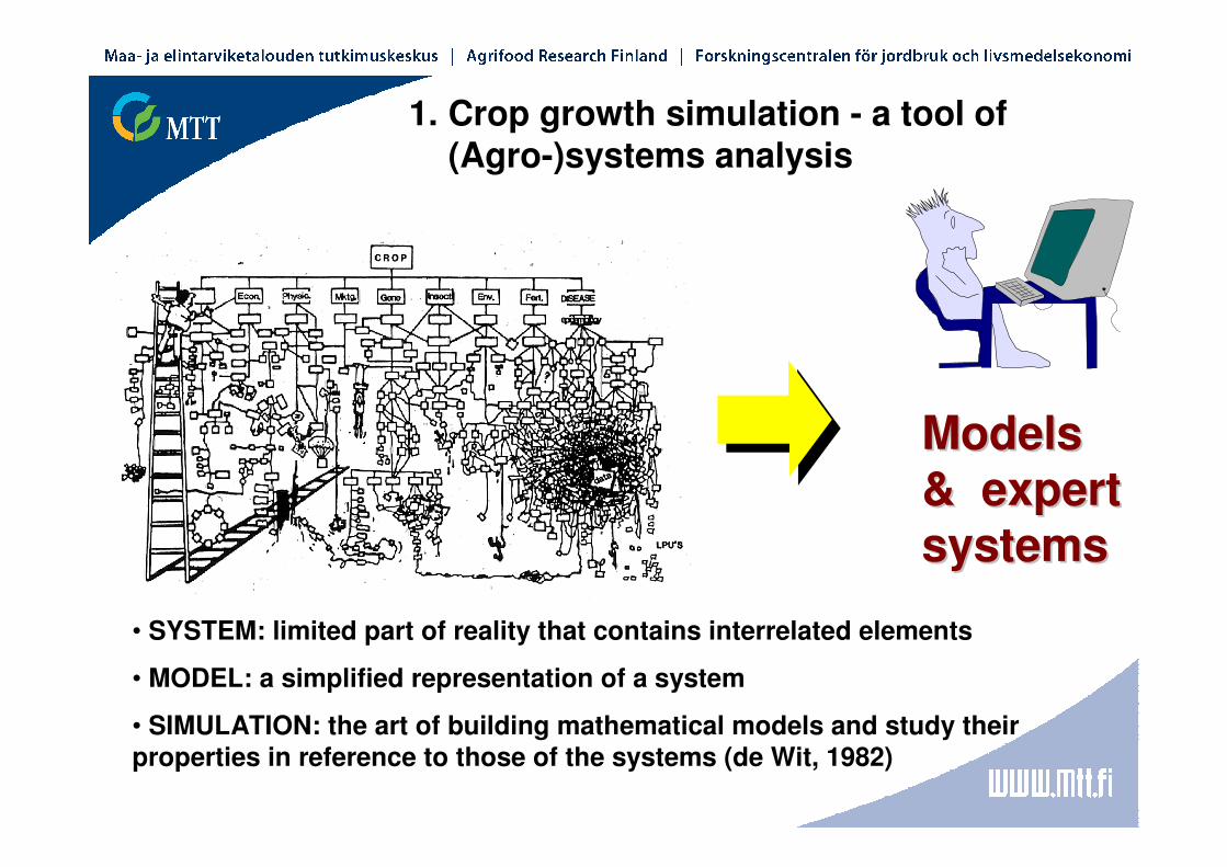
• SYSTEM: limited part of reality that contains interrelated elements

• MODEL: a simplified representation of a system

• SIMULATION: the art of building mathematical models and study their properties in reference to those of the systems (de Wit, 1982)

1. Crop growth simulation - a tool of (Agro-)systems analysis

4

1. Crop growth simulation

Why is dynamic crop growth simulation useful ?

• Generally : (i) to disentangle and explain effects of yield-determining /–limiting and reducing factors; (ii) to integrate fragmented agronomic with biophysical data & extrapolate in time & space

• In climate change impact and adaptation research: their capability allows analysis of crop response to T, P (SM), CO2 and changed management conditions

• => Pre-requisite : Proper evaluation (calibration, sensitivityanalysis, validation..)

5

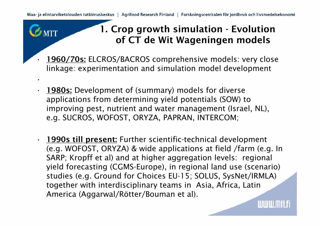
1. Crop growth simulation - Evolution of CT de Wit Wageningen models

• 1960/70s: ELCROS/BACROS comprehensive models: very close linkage: experimentation and simulation model development

•

• 1980s: Development of (summary) models for diverse applications from determining yield potentials (SOW) to improving pest, nutrient and water management (Israel, NL), e.g. SUCROS, WOFOST, ORYZA, PAPRAN, INTERCOM;

• 1990s till present: Further scientific-technical development (e.g. WOFOST, ORYZA) & wide applications at field /farm (e.g. InSARP; Kropff et al) and at higher aggregation levels: regional yield forecasting (CGMS-Europe), in regional land use (scenario) studies (e.g. Ground for Choices EU-15; SOLUS, SysNet/IRMLA) together with interdisciplinary teams in Asia, Africa, Latin America (Aggarwal/Rötter/Bouman et al).

6

1. Crop growth simulation - capabilities and limitations. Hierarchical modeling

approach of C.T. de Wit School

7

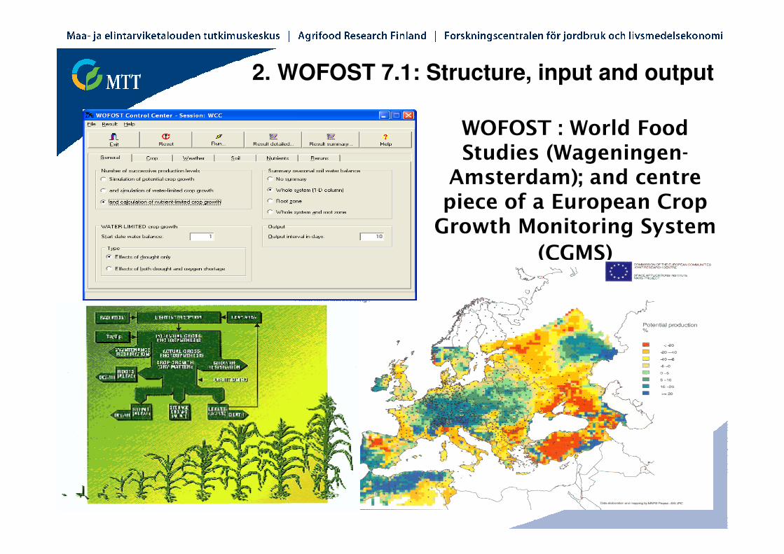
WOFOST : World Food Studies (Wageningen-

Amsterdam); and centre piece of a European Crop Growth Monitoring System

(CGMS)

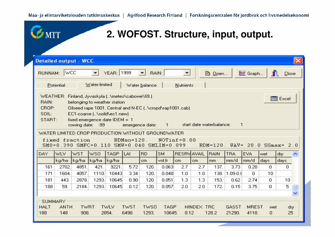
2. WOFOST 7.1: Structure, input and output

8

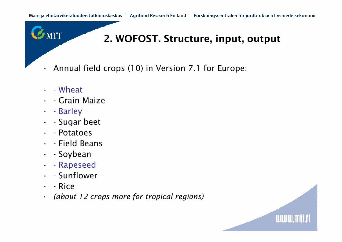
2. WOFOST. Structure, input, output

• Annual field crops (10) in Version 7.1 for Europe:

• - Wheat

• - Grain Maize

• - Barley

• - Sugar beet

• - Potatoes

• - Field Beans

• - Soybean

• - Rapeseed

• - Sunflower

• - Rice• (about 12 crops more for tropical regions)

9

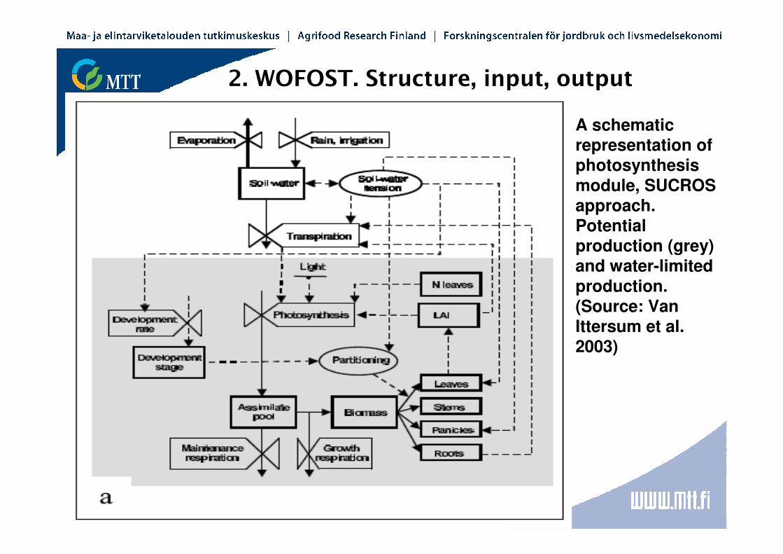
2. WOFOST. Structure, input, output

A schematic

representation of photosynthesis

module, SUCROS

approach. Potential

production (grey)

and water-limited

production. (Source: Van

Ittersum et al.

2003)

10

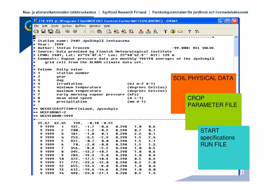
SOIL PHYSICAL DATA

CROP

PARAMETER FILE

START

specifications

RUN FILE

11

12

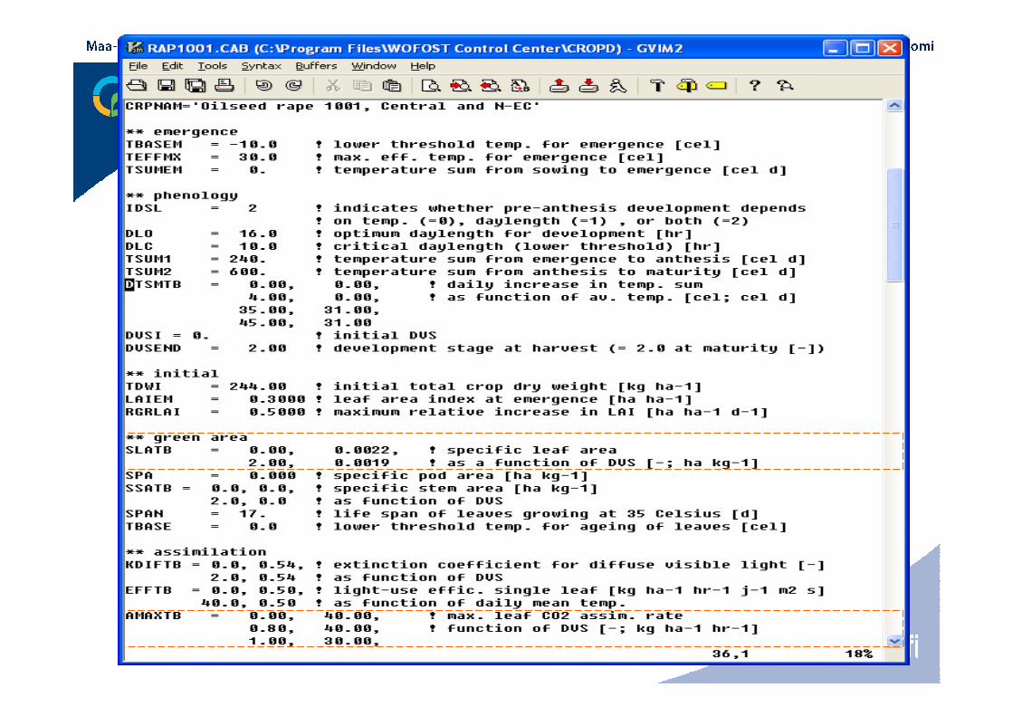
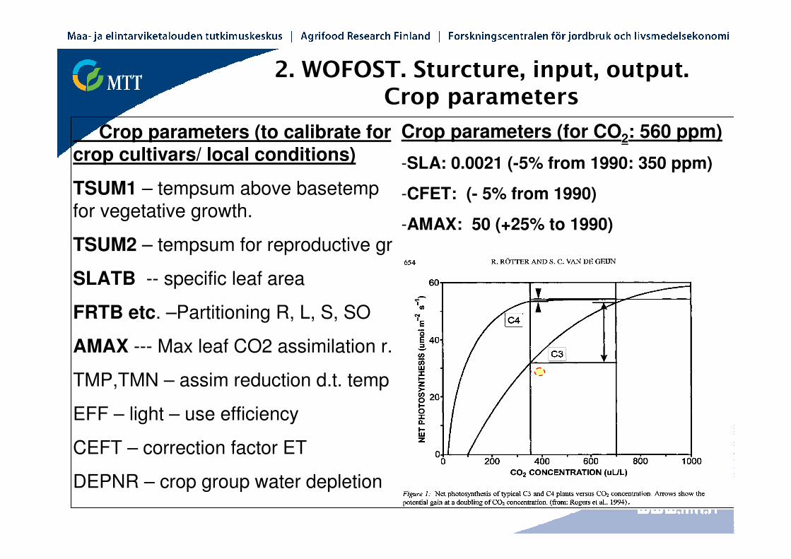
2. WOFOST. Sturcture, input, output. Crop parameters

Crop parameters (for CO2: 560 ppm)

-SLA: 0.0021 (-5% from 1990: 350 ppm)

-CFET: (- 5% from 1990)

-AMAX: 50 (+25% to 1990)

Crop parameters (to calibrate for crop cultivars/ local conditions)

TSUM1 – tempsum above basetemp for vegetative growth.

TSUM2 – tempsum for reproductive gr

SLATB -- specific leaf area

FRTB etc. –Partitioning R, L, S, SO

AMAX --- Max leaf CO2 assimilation r.

TMP,TMN – assim reduction d.t. temp

EFF – light – use efficiency

CEFT – correction factor ET

DEPNR – crop group water depletion

13

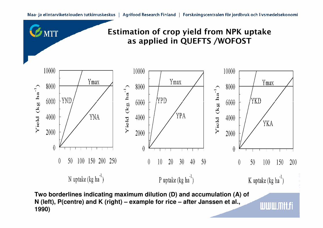
Estimation of crop yield from NPK uptake as applied in QUEFTS /WOFOST

Two borderlines indicating maximum dilution (D) and accumulation (A) of

N (left), P(centre) and K (right) – example for rice – after Janssen et al.,

1990)

14

2. WOFOST. Structure, input, output.

15

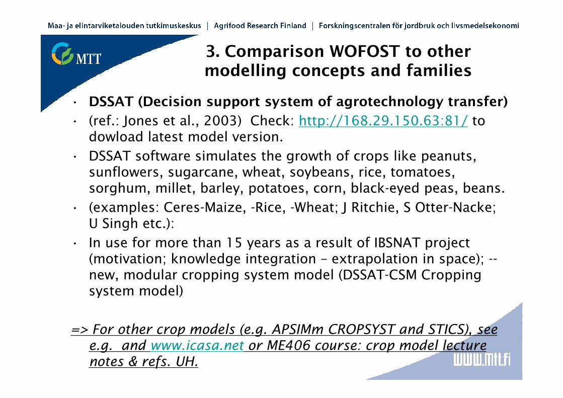
3. Comparison WOFOST to other modelling concepts and families

• DSSAT (Decision support system of agrotechnology transfer)

• (ref.: Jones et al., 2003) Check: http://168.29.150.63:81/ to dowload latest model version.

• DSSAT software simulates the growth of crops like peanuts, sunflowers, sugarcane, wheat, soybeans, rice, tomatoes, sorghum, millet, barley, potatoes, corn, black-eyed peas, beans.

• (examples: Ceres-Maize, -Rice, -Wheat; J Ritchie, S Otter-Nacke; U Singh etc.):

• In use for more than 15 years as a result of IBSNAT project (motivation; knowledge integration – extrapolation in space); --new, modular cropping system model (DSSAT-CSM Cropping system model)

=> For other crop models (e.g. APSIMm CROPSYST and STICS), see e.g. and www.icasa.net or ME406 course: crop model lecture notes & refs. UH.

16

3. Comparison WOFOST to other modelling concepts and families

• Development stages (driving variables: Temp/cultivar; co-determining factors (e.g. daylength in Wofost; soil temp or soil moisture in CERES?......);

• Assimilation and dry matter increase (processes: leaf photosynthesis, LAI, maintenance and growth respiration (SUCROS approach); descriptive: light interception – dry matter relationship; ---- effect CO2 concentration on photosynthesis (via AMAX and EFF)

• Partitioning of assimilates /dry matter to different plant organs (dev. stage dependent, fixed fractions or ?. Root : shoot (and leaf: stem: storage organs);

• Leaf area development (calc. from leaf dry weight, specific leaf area for closed canopy; exponential growth – unclosed.. ends at LAI 1; dependency on temperature; rel. Leaf death rate --- vs green area )

• Soil water balance (tipping bucket/cascading or Richards approach; no. of layers, ETo e.g. According to Penman)

• Nutrient – limitation (Static QUEFTS approach for NPK in WOFOST; dynamic N appproach; comprehensive approaches in CERES/DSSAT-CSM, HERMES...)

17

4. How to evaluate ?

Statistical evaluation of model performance (as recommended by e.g. Willmott 1981):

• - Summary measures: observed and predicted means, STD, sample size, intercept and slope of simple regression between dependentand independent(=oberved) variable; and coefficient of determination

• - Difference measures: mean absolute error MAE, mean square error MSE, systematic and unsystematic parts of MSE and RMSE, and the index of agreement (d)

Apply models judiciously; scientist with background in major related disciplines – models are not fool-proof...............,

Combine, whenever possible, experimentation and modelling

18

4. How to evaluate ?

• Calibration, sensitivity analysis, validation

• - calibration: essential step in model development aimed at adjusting or deriving parameter values on the basis of experimental data --procedure (see, successive steps for crop models ); calibration can take site differences and minor ecological processes into account, it is essential to reduce calibration for that purpose (of curve fitting)

• - sensitivity analysis: as a form of behavioral analysis and part of model evaluation, carried out in order to assess the influence of selected key (’critical’) parameters on, usually, most important output variables (sensitivity indicators) – what-if; irrespective of real system behaviour;

• - validation: the examination whether a model derived from the analyses of some systems is capable of describing other systems – or, in the narrow sense, how well the model outputs fit (new) data (de Wit, 1982; Joergensen, 1983); � most difficult step in evaluation

19

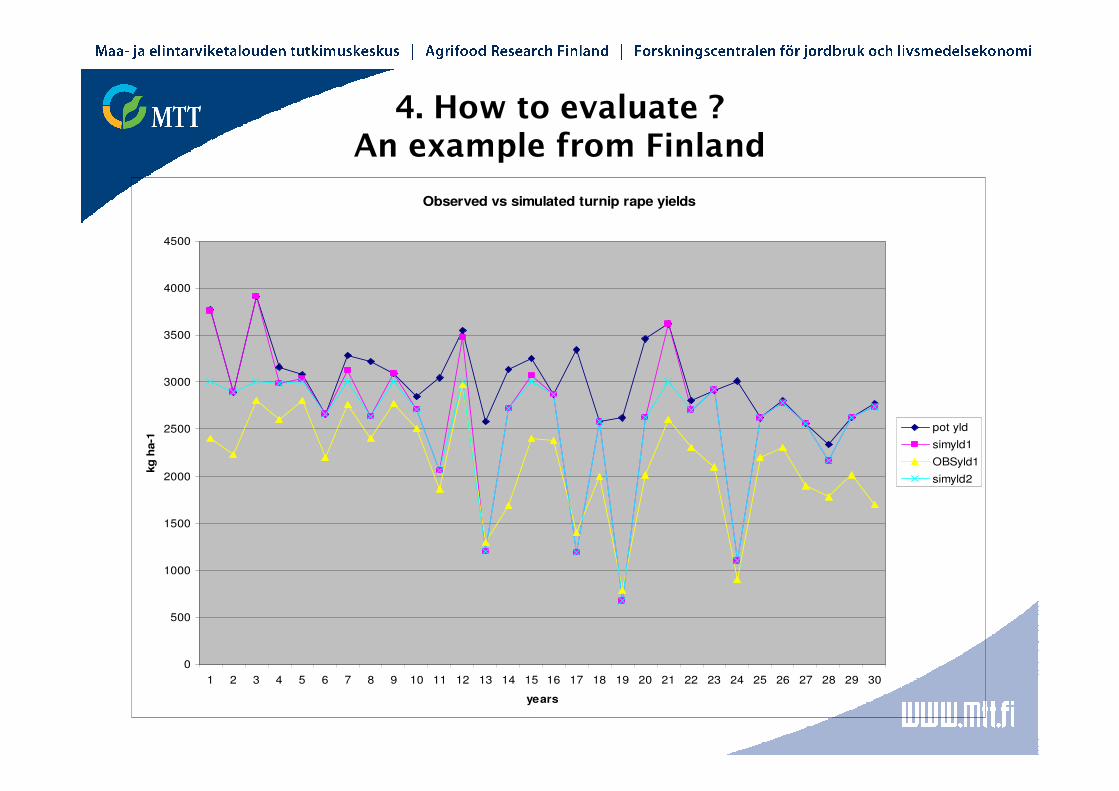
4. How to evaluate ? An example from Finland

Observed vs simulated turnip rape yields

0

500

1000

1500

2000

2500

3000

3500

4000

4500

1 2 3 4 5 6 7 8 9 10 11 12 13 14 15 16 17 18 19 20 21 22 23 24 25 26 27 28 29 30

years

kg

ha-1

pot yld

simyld1

OBSyld1

simyld2

20

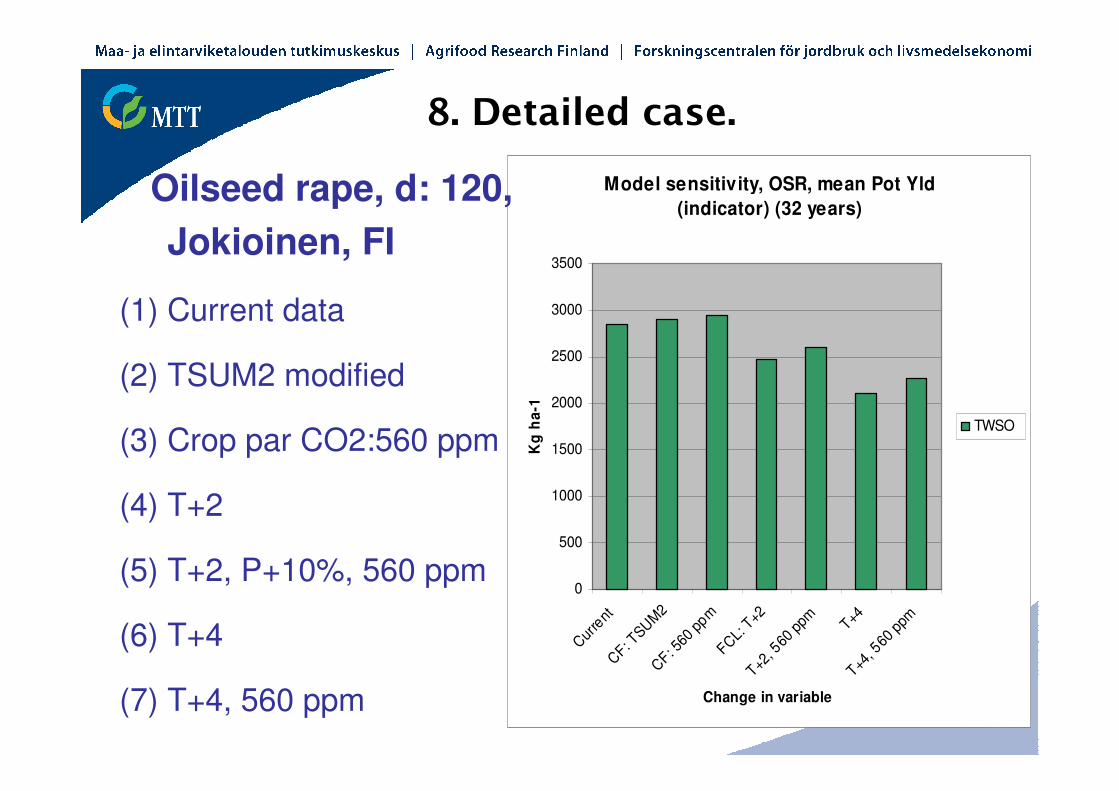
8. Detailed case.

Model sensitivity, OSR, mean Pot Yld

(indicator) (32 years)

0

500

1000

1500

2000

2500

3000

3500

Cur

rent

CF: T

SUM

2C

F: 560

ppm

FCL:

T+2

T+2, 5

60 p

pm T+4T+4

, 560

ppm

Change in variable

Kg

ha

-1

TWSO

Oilseed rape, d: 120,

Jokioinen, FI

(1) Current data

(2) TSUM2 modified

(3) Crop par CO2:560 ppm

(4) T+2

(5) T+2, P+10%, 560 ppm

(6) T+4

(7) T+4, 560 ppm

21

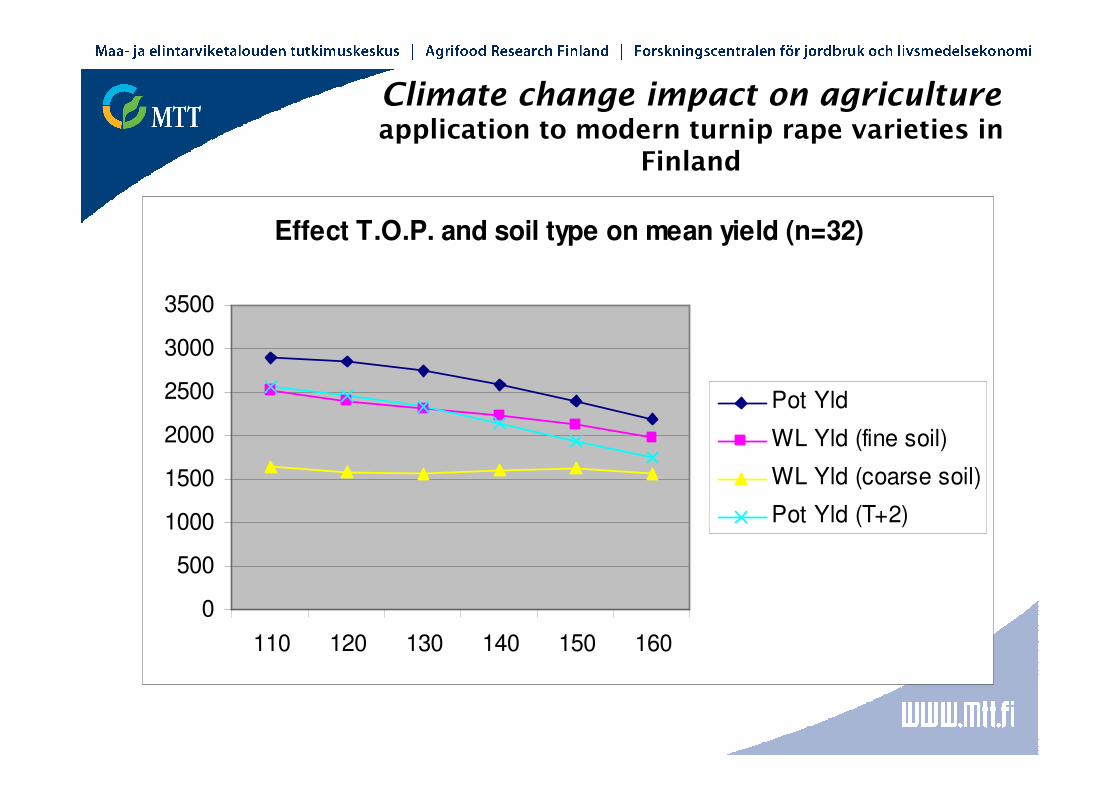
Climate change impact on agriculture application to modern turnip rape varieties in

Finland

Effect T.O.P. and soil type on mean yield (n=32)

0

500

1000

1500

2000

2500

3000

3500

110 120 130 140 150 160

Pot Yld

WL Yld (fine soil)

WL Yld (coarse soil)

Pot Yld (T+2)

22

(Averaged) yield changes for major crops in the Rhine Basin (scenario BAU-best)

• Simulated water-limited yield increase

• yield (t ha-1) (%)

• current future

• ___________________________________________________________________

• winter wheat 7.0 9.5 35.7

• potato 10.6 12.4 17.0

• sugarbeet 12.7 16.0 26.0

• silage maize 17.6 20.0 14.0

• ryegrass 14.7 19.4 32.0

• (Lolium perenne)

• ___________________________________________________________________

•

23

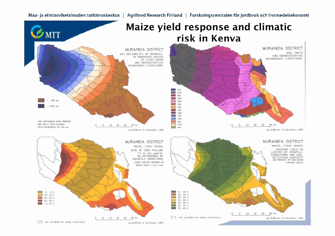
Maize yield response and climaticrisk in Kenya