Embed Size (px)
Citation preview

American Journal of Computational and Applied Mathematics 2013, 3(4): 238-249 DOI: 10.5923/j.ajcam.20130304.07
Modified Estimators for Some Noisy Dynamical Systems
Salah H Abid*, Shahad S Al-Azawie
Al-Mustansirya University – Education College-Mathematics Dept
Abstract Lele in (1994)[8], Used the estimat ing function method to analyze and estimate the exponential and the logistic noisy dynamical systems. also, He used simulat ion to study the small-sample properties. Hassan in (2012)[7], derived an estimator o f the Tent noisy dynamical system based on estimating function method. In th is paper we will modify Lele̕s estimator of noisy logistic and noisy exponential dynamical systems and Hasan̕s estimator of noisy tent dynamical system, to be more efficient based on a simulat ion experiment. The results shows that the modified estimators performs better than unmodified estimators based on the mean square error criterion.
Keywords Lele's estimator, Hassan's estimstor, Noisy dynamical system
1. Introduction The dynamical system is a mathemat ic formula describes
changes of an initial state space for the time. Which could be discrete or continuous. In the noisy dynamical system we can define the "noisy chaotic" by using stochastic Lyapunov exponent (SLE).
Godambe (1984)[4], Studied utilizing the theory of estimating equations[3], this paper develops concepts of parameter defin ing function and effective parameter. The paper provides theory and techniques for choosing from a given set of robust parameters one that is most effective, or one that can most efficiently be estimated.
Berliner (1991)[2], Studied statistical prediction for dynamical system with error.considered parametric models that lead to chaos on a subset of the parameter space. He considered a likelihood based approach for estimation of the parameters of the underlying determin istic system in the presence of measurement error. He also considered Bayesian prediction for these so called "unpredictable processes" , also he suggested some novel characteristics of chaotic data analysis.
Hassan (2012)[7], Compare among some of the methods used to estimate these models by using simulat ion. and propose an asymmetric dynamical system which is based on a mixture of two maps (asymmetric logistic and asymmetric tent).
In this research we are interested of noisy Dynamical systems according to logistic, exponential, and tent maps, so we will introduce then as follows.
* Corresponding author: [email protected] (Salah H Abid) Published online at http://journal.sapub.org/ajcam Copyright © 2013 Scientific & Academic Publishing. All Rights Reserved
2. Estimating Function Method Estimating function[5], have proved to be a promising
alternative to the maximum likelihood estimat ion. they usually lead to simple numerical calculat ions and also posses a robustuess property[4], In that they need only the specification of the first few, usually two, moments instead of the complete specification of the underlying distribution.
In the fo llowing we briefy describe the estimat ing function approach and then apply it to the three maps logistic, exponential, and tent.
Let θ be a one dimensional parametre taking values in Θ. Let 𝒳𝒳 denote the sample space. An estimating function for θ is defined[3] as any function ƒ: 𝒳𝒳 x Θ → ℛ such that EΘ [ƒ(y,θ)] =0.
An estimator 𝜃𝜃^ is obtained by solving the empirical version ƒ(y,θ)=0 under suilab le regularity conditions. These estimators are consist and asymptotically normal.
1) Logistic map with additive Gaussion noise. The dynamical system of the logistic map is .[10]
𝐺𝐺a(𝒳𝒳) = 𝒳𝒳𝑡𝑡+1 = a 𝒳𝒳𝑡𝑡 (1-𝒳𝒳𝑡𝑡 ) (1)
Where all t in T= {0,1,2,…}, 𝒳𝒳𝑡𝑡 ∈[0,1], and a∈[0,4]. The above dynamical system has the following
properties.[10] a) If 0 < a < 1 then the system has one fixed point q=0 is a
stable. b) if 1 < a < 3 then the system has two fixed point q1=0 is
unstable and q2= 1-(1/a) is stable and appears 1-cycle. c) if 3 < a < 3.449 then the system has one fixed point q =
1-(1/a) unstable and appers 2-cycles. d) if a=3.57 then the system becomes chaotic. The noisy dynamical system of logistic map.[8]

American Journal of Computational and Applied Mathematics 2013, 3(4): 238-249 239
𝐺𝐺𝑎𝑎 (Yt,ɳ𝑡𝑡 ) =Yt+1 = 𝒳𝒳𝑡𝑡+1 + ɳ t (2)
Where Ga: ℛ x → ℛ, a ∈[0,4], and {ɳt} (iid) random varible we assume that ɳt ∼ Gauss (0,𝜎𝜎2).
Bifurcation diagram of the system (1) and (2) are in figures (1-a) and (1-b).
(a)
(b)
Figure (1). The bifurcation diagram of the logistic system, x-axis represent the values of a and y-axis represent the values of Хt+1. (a) in deterministic case, (b) in noisy case with additive Gaussian(0, 0.0025) noise
2) Exponential map with multiplicative log-Gaussian noise.
The dynamical system of the exponential map[9] Ea(𝒳𝒳𝑡𝑡 ) = 𝒳𝒳𝑡𝑡+1 = 𝒳𝒳𝑡𝑡 exp (a(1-𝒳𝒳𝑡𝑡 )) (3)
Where all t in T={0,1,2,…}, 𝒳𝒳𝑡𝑡 ∈[0,∞), and a ∈ (0,∞) The above dynamical system has the following properties.
[9] a) If 0 < a < 2 Then the system has two fixed point
q1=0 is unstable and q2=1 is stable. b) If 2 < a < 2.44 Then the system has two fixed point
q1=0 and q2=1 bath are unstable. c) If a=2.6924 Then the system chaotic. The noisy dynamical system of the exponential map.[8]
Ea( Yt ,𝘡𝘡t) = Yt+1 = 𝒳𝒳𝑡𝑡+1 𝘡𝘡t (4)
Where Ea:[0,∞) x →[0,∞), a ∈ (0,∞), and {𝘡𝘡t} iid random variables we assume that 𝘡𝘡t ∼ log Gauss (−𝜎𝜎
2
2, 𝜎𝜎2).
Bifurcation diagram of the system (3) and (4) are in figures (2-a) and (2-b).
(a)
(b)
Figure (2). The bifurcation diagram of the Exponential system, x-axis represent the values of a and y-axis represent the values of Хt+1. (a) in deterministic case, (b) in noisy case with additive log Gaussian(-0.05, 0.1) noise
3) Tent map with additive Gassus noise The dynamical system of the tent map.[6]
Ta(𝒳𝒳𝑡𝑡 ) = 𝒳𝒳𝑡𝑡+1 = �2𝑎𝑎 𝒳𝒳𝑡𝑡 𝑖𝑖𝑖𝑖 0 < 𝑎𝑎 < 1
2
2𝑎𝑎 (1 − 𝒳𝒳𝑡𝑡 ) 𝑖𝑖𝑖𝑖 12
< 𝑎𝑎 < 1� (5)
Where all t in T={0,1,2,...}, 𝒳𝒳𝑡𝑡 ∈[0,1] , and a ∈[0,1] The above dynamical system has the following
properties.[6] a) if 0 < a < 1/2 then the system has one fixed point q =0 is
stuble. b) if a=1/2, if 0 ≤ 𝒳𝒳 ≤ 1/2 then all points represent fixed
points and if 1/2 ≤ 𝒳𝒳 ≤ 1 then all points represent eventually fixed points.

240 Salah H Abid et al.: Modified Estimators for Some Noisy Dynamical Systems
c) If 1/2 ≤ a ≤ 1 then the system has two fixed point q1=0 and q2= 2𝑎𝑎
1 +2𝑎𝑎 both are unstuble and the system becomes
chaotic. The noisy dynamical system of the tent map
Ta(Yt,ɳt) = Yt+1 = �2𝑎𝑎𝒳𝒳𝑡𝑡 + ɳ𝑡𝑡 𝑖𝑖𝑖𝑖 𝒳𝒳𝑡𝑡 < 1
2
2𝑎𝑎(1 − 𝒳𝒳𝑡𝑡) + ɳ𝑡𝑡 𝑖𝑖𝑖𝑖 𝒳𝒳𝑡𝑡 > 12
� (6)
Where Ta: ℛ x → ℛ , a∈[0,1], and {ɳ t} iid random variable , we assume that ɳt∼ Gauss (0,𝜎𝜎2) as in the logistic system.
Bifurcation diagram of the system (5) and (6) are in figures (3-a) and (3-b).
(a)
(b)
Figure (3). The bifurcation diagram of the Tent system, x-axis represent the values of a and y-axis represent the values of Хt+1. (a) in deterministic case, (b) in noisy case with additive Gaussian(0, 0.0025) noise
3. Measurement Error Since the calculat ion of the parameter values is triv ial, the
practical calculation of anoise introduced series
{Yt,t=0,1,2,…} , can be done using the mesnring device by two kinds of mesurment erro rs.
(1) Additive error. Here Yt = 𝒳𝒳𝑡𝑡 + 𝜎𝜎ɳ𝑡𝑡 , 𝜎𝜎 > 0, where ɳ𝑡𝑡 ’𝑠𝑠 are independent identically distributed random variables with mean 0 and variance 1. [3] assumed these to be Gaussian.
(2) Mult iplicative error. Here Yt = 𝒳𝒳𝑡𝑡+1 𝘡𝘡t; where 𝘡𝘡t‘s are independent identically random variables with mean 1, variance 𝜎𝜎2 , and range on[0,∞).
By apply ing the estimating function method on the logistic and exponential system Lele derived the Following[8],
i) For a noisy logistic dynamical system, he wrote, ƒ(y,a)= ∑ (𝑦𝑦𝑡𝑡 +1−𝑛𝑛−1𝑡𝑡=0 a(𝑦𝑦𝑡𝑡 − 𝑦𝑦𝑡𝑡2 + 𝜎𝜎2)) and then got the EF estimator
of as
â= ∑ 𝑦𝑦𝑡𝑡+1𝑛𝑛−1𝑡𝑡=0
∑ (𝑦𝑦𝑡𝑡−𝑦𝑦𝑡𝑡2+𝜎𝜎2 )𝑛𝑛−1𝑡𝑡=0
(7)
ii) For a noisy dynamical exponential system, he wrote. ƒ(y,a)=∑ {[(𝑙𝑙𝑙𝑙𝑙𝑙𝑌𝑌𝑡𝑡+1 − 𝑙𝑙𝑙𝑙𝑙𝑙𝑌𝑌𝑡𝑡𝑛𝑛−1
𝑡𝑡=0 )2 −2𝜎𝜎2 ]−𝑎𝑎2 (1−2𝑌𝑌𝑡𝑡 + 𝑌𝑌𝑡𝑡1 +𝑒𝑒𝜎𝜎2 )}
and then got the EF estimator of as
â = abs[∑ (log 𝑦𝑦𝑡𝑡+1−𝑙𝑙𝑙𝑙𝑙𝑙𝑦𝑦𝑡𝑡𝑛𝑛−1𝑡𝑡=0 )2−𝜎𝜎2
∑ (1−2𝑦𝑦𝑡𝑡𝑛𝑛−1𝑡𝑡=0 + 𝑦𝑦𝑡𝑡
1+𝑒𝑒𝜎𝜎2)]1/2 (8)
(iii) By using the same argument Hassan in 2012 derived the estimator of the parameter of noisy tent dynamical system to be[7],
â= 𝑛𝑛2∑ 𝑦𝑦𝑡𝑡+1𝑛𝑛−1𝑡𝑡=0
𝑛𝑛 ∑ 𝑦𝑦𝑡𝑡−∑ 𝑦𝑦𝑡𝑡2𝑛𝑛−1𝑡𝑡=0
𝑛𝑛−1𝑡𝑡=0
(9)
4. The Empirical Study A simulat ion experiment was conducted to modify the
estimating function estimator of parameter of logistic, exponential and tent random dynamical system. We wrote the programs for this goal by asing Matlab R2008a, with run size equal to 500.
After execute the Simulat ion experiment, we got a tremendous amount of results. These results are summarized in tables, but put these tables in this research was inappropriate because of their big magnitude . As Possible alternative,we summed up these results in figures.
Figures (4.a),(4.b),(5.a),(5.b),(6.a) and (6.b) for logistic map, figures (7.a),(7.b),(8.a),(8.b),(9.a) and (9.b) for exponential map and figures (10.a),(10.b),(11.a),(11.b),(12.a) and (12.b) for tent map.
If any person wish, it is possible to email us to provide the results tables of the simulat ion experiment.
The figures show us the clear differences between the real values of a and their estimates (depending of the lele's estimators for the cases of logistic and exponential maps and hassan's estimator for tent map) , especially in the cases of tent and exponential maps . So, as a goal of our work, we took upon ourselves the issue of modification of lele's and hassan's estimators

American Journal of Computational and Applied Mathematics 2013, 3(4): 238-249 241
Following the results we reached 1) Figures (4), (5) and (6) represent the estimations of the
parameter o f the noisy logistic dynamical system for the following combinations of 𝜎𝜎2 , a, and L, where 𝜎𝜎2 is the variance of the noisy variant, a is the bifurcation parameter of the logistic system and L is the length of the noisy orbit.
Following the values of 𝜎𝜎2 , a and L used in simulation experiment, to get Lele’s estimator of noisy logistic dynamical system, 𝜎𝜎2= 0.01, 0.16 , 0.25, a = 0.25 , 0.5 , 1, 1.5, 1.75, 2 , 2.25 , 2.5 , 3 , 3.75, 3.95 , 4 and L=20, 35, 50, 65, 85, 100, 160, 220, 280, 340, 400, 500, 550, 600, 650, 700, 750, 800, 850, 1000.
According to the results one can easly modify Lele̕s estimator of a in the noisy Logistic dynamical system to be ã𝐿𝐿= 0.948759 â – 0.098929 𝜎𝜎2 + 0.00000606 L.
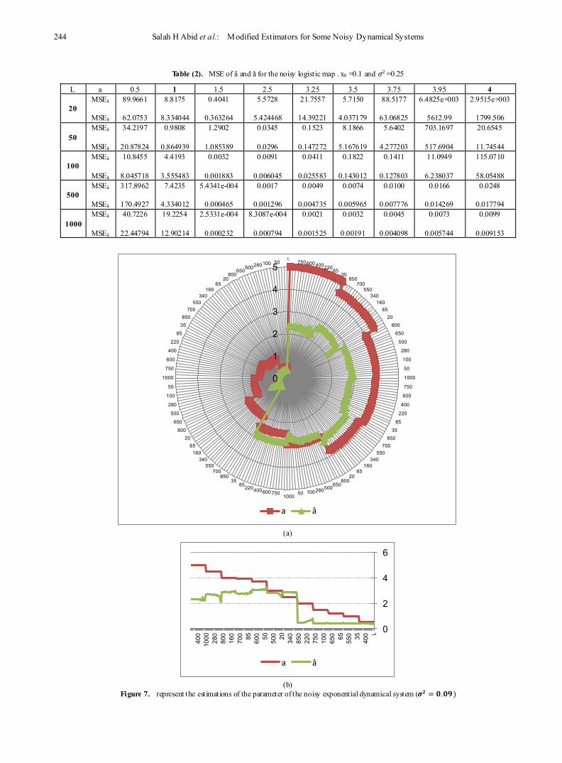
2) Figures (7), (8) and (9) represent the estimations of the parameter of the noisy exponential dynamical system for the following combinations of 𝜎𝜎2 , a and L, where 𝜎𝜎2 is the variance of the noisy variant, a is the bifurcation parameter of the exponential system and L is the length of the noisy orbit.
Following the values of 𝜎𝜎2 , a and L used in simulation experiment to get Lele’s estimator of noisy exponential dynamical system, 𝜎𝜎2= 0.09, 0.21 , 0.36, a = 0.5 , 1 , 1.25, 1.5, 2 , 2.5 ,3 , 3.75, 3.95 , 4 , 4.5 , 5 and L =20 , 35 , 50 , 65 ,
85 , 100 , 160 , 220 , 280, 340, 400 , 500, 550 , 600, 650 , 700 , 750 , 800 , 850 , 1000.
According to the above results one can easly modify Lele̕s estimator of a in the noisy Exponential dynamical system to be ãE = 1.092332 â + 0.0083 𝜎𝜎2 + 0.00025 L
3) Figures (10), (11) and (12) represent the estimations of the parameter of the noisy tent dynamical system for the following combinations of 𝜎𝜎2 , a, and L, where 𝜎𝜎2 is the variance of the noisy variant, a is the bifurcation parameter of the tent system and L is the length of the noisy orbit.
Following the values of 𝜎𝜎2 , a, and L used in simulation experiment to get Hassan’s estimator o f noisy tent dynamical system, 𝜎𝜎2= 0.01 , 0.16 , 0.25, a = 0.25 , 0.5, 1, 1.5, 1.75, 2 , 2.25 , 2.5 , 3 , 3.75, 3.95 , 4 and L=20, 35, 50, 65, 85, 100, 160, 220, 280, 340, 400, 500, 550, 600, 650, 700, 750, 800, 850, 1000.
According to the above results one can easly modify Hassan’s estimator of a in the noisy Tent dynamical system to be ãT = 0.9432 â + 0.27 𝜎𝜎2 + 0.000043 L
4) An additional Experiments was conducted to compare between â and ã for noisy logistic, noisy exponential and noisy tent dynamical systems in different situations.
Tables (1), (2), (3), (4), (5) and (6) contain the mean square error results. It is clear that the performance of ã is better than the performance of â.
(a)
0
1
2
3
4
5 L
50 100 280 500 650
800 20
65 160
340 550
700 850
35
85
220
400
600
750
1000
50
100
280
500
650
800
20 65
160 340
550 700
850 35
85 220 400 600 750
1000 50 100 280 500
650 800
20 65
160 340
550 700
850
35
85
220
400
600
750
1000
50
100
280
500
650
800
20 65
160 340
550 700
850 35
85 220 400 600 750
a â

242 Salah H Abid et al.: Modified Estimators for Some Noisy Dynamical Systems
(b) Figure 4. represent the estimations of the parameter of the noisy Logistic dynamical system (𝝈𝝈𝟐𝟐 = 𝟎𝟎.𝟎𝟎𝟎𝟎)
(a)
(b)
Figure 5. represent the estimations of the parameter of the noisy Logistic dynamical system (𝝈𝝈𝟐𝟐 = 𝟎𝟎.𝟎𝟎𝟏𝟏)
0
1
2
3
4
5
L 40
0
35 550
65 650
100
750
220
850
340
20 500
50 600
85 700
160
800
280
1000
40
0
a â
0
1
2
3
4
5
6 L
50 100 280 500 650 800
20 65
160 340
550 700
850 35
85
220
400
600
750
1000
50
100
280
500
650 800
20 65
160 340
550 700
850 35
85 220 400 600 750 1000
50 100 280 500 650 800
20 65
160 340
550 700
850 35
85
220
400
600
750
1000
50
100
280
500
650 800
20 65
160 340
550 700
850 35
85 220 400 600 750
a â
0 1 2 3 4 5 6 7
L 34
0 10
00
340
1000
34
0 10
00
340
1000
34
0 10
00
340
1000
34
0 10
00
340
1000
34
0 10
00
340
1000
34
0 10
00
340
a â

American Journal of Computational and Applied Mathematics 2013, 3(4): 238-249 243
(a)
(b)
Figure 6. represent the estimations of the parameter of the noisy Logistic dynamical system (𝝈𝝈𝟐𝟐 = 𝟎𝟎.𝟐𝟐𝟐𝟐)
Table (1). MSE of â and ã for the noisy logistic map. x0 =0.1 and 𝜎𝜎2 =0.01
4 3.95 3.75 3.5 3.25 2.5 1.5 1 0.5 a L 0.0232
0.012844
0.0064
0.004654
0.0057
0.004247
0.0042
0.002255
0.0024
0.002159
7.4934e-004
0.000648
1.6066e-004
0.00015
0.0018
0.001487
2.3210
1.301327
MSE â
MSEã 20
0.0055
0.004302
0.0025
0.001919
0.0017
0.001644
0.0012
0.001174
7.6522e-004
0.000505
2.7885e-004
0.000275
4.3429e-005
3.33E-05
0.0015
0.001278
0.0915
0.089236
MSE â
MSEã 50
0.0023
0.001774
0.0013
0.001129
8.8806e-004
0.000514
6.3375e-004
0.000423
4.5336e-004
0.00033
1.3350e-004
0.000111
2.1796e-005
1.9E-05
9.2401e-004
0.000787
0.1444
0.120662
MSE â
MSEã 100
4.1657e-004
0.000305
2.6942e-004
0.000166
1.5598e-004
0.00013
1.3079e-004
0.000114
8.4720e-005
6.63E-05
3.1406e-005
2.38E-05
4.2058e-006
3.72E-06
0.0586
0.030925
31.9170
22.75633
MSE â
MSEã 500
1.8837e-004
0.000183
1.4182e-004
0.000118
8.8197e-005
5.69E-05
5.8172e-005
5.79E-05
4.0029e-005
3.14E-05
1.4131e-005
9.63E-06
2.0052e-006
1.06E-06
0.0292
0.021681
0.0564
0.031825
MSE â
MSEã 1000
0
1
2
3
4
5
6 L
50 100 280 500 650
800 20
65 160
340 550
700 850
35
85
220
400
600
750
1000
50
100
280
500
650
800
20 65
160 340
550 700
850 35
85 220 400 600 750
1000 50 100 280 500
650 800
20 65
160 340
550 700
850
35
85
220
400
600
750
1000
50
100
280
500
650
800
20 65
160 340
550 700
850 35
85 220 400 600 750
a â
0 1 2 3 4 5 6
L 40
0
35 550
65 650
100
750
220
850
340
20 500
50 600
85 700
160
800
280
1000
40
0
a â
244 Salah H Abid et al.: Modified Estimators for Some Noisy Dynamical Systems
Table (2). MSE of â and ã for the noisy logistic map . x0 =0.1 and 𝜎𝜎2 =0.25 4 3.95 3.75 3.5 3.25 2.5 1.5 1 0.5 a L
2.9515e+003
1799.506
6.4825e+003
5612.99
88.5177
63.06825
5.7150
4.037179
21.7557
14.39221
5.5728
5.424468
0.4041
0.363264
8.8175
8.334044
89.9661
62.0753
MSEâ
MSEã 20
20.6545
11.74544
703.1697
517.6904
5.6402
4.277203
8.1866
5.167619
0.1523
0.147272
0.0345
0.0296
1.2902
1.085389
0.9808
0.864939
34.2197
20.87824
MSEâ
MSEã 50
115.0710
58.05488
11.0949
6.238037
0.1411
0.127803
0.1822
0.143012
0.0411
0.025583
0.0091
0.006045
0.0032
0.001883
4.4193
3.555483
10.8455
8.045718
MSEâ
MSEã 100
0.0248
0.017794
0.0166
0.014269
0.0100
0.007776
0.0074
0.005965
0.0049
0.004735
0.0017
0.001296
5.4341e-004
0.000465
7.4235
4.334012
317.8962
170.4927
MSEâ
MSEã 500
0.0099
0.009153
0.0073
0.005744
0.0045
0.004098
0.0032
0.00191
0.0021
0.001525
8.3087e-004
0.000794
2.5331e-004
0.000232
19.2254
12.90214
40.7226
22.44794
MSEâ
MSEã 1000
(a)
(b)
Figure 7. represent the estimations of the parameter of the noisy exponential dynamical system (𝝈𝝈𝟐𝟐 = 𝟎𝟎.𝟎𝟎𝟎𝟎)
0
1
2
3
4
5 L
50 100 280 500 650 800
20 65
160 340
550 700
850 35
85
220
400
600
750
1000
50
100
280
500
650
800 20
65 160
340 550
700 850
35 85 220 400 600 750
1000 50 100 280 500 650
800 20
65 160
340 550
700 850
35
85
220
400
600
750
1000
50
100
280
500
650
800 20
65 160
340 550
700 850
35 85 220 400 600 750
a â
0
2
4
6
L 40
0
35 550
65 650
100
750
220
850
340
20 500
50 600
85 700
160
800
280
1000
40
0
a â

American Journal of Computational and Applied Mathematics 2013, 3(4): 238-249 245
(a)
(b)
Figure 8. represent the estimations of the parameter of the noisy exponential dynamical system (𝝈𝝈𝟐𝟐 = 𝟎𝟎.𝟐𝟐𝟎𝟎)
Table (3). MSE of â and ã for the noisy exponential map, x0=1.3 and 𝜎𝜎2 =0.09
4.5 3.95 3.75 3.5 3.25 3 2.5 2 1.5 1 a L 54.2231
28.9951
52.2230
28.91195
23.2288
21.0158
0.0730
0.054396
0.5261
0.282436
0.0585
0.052616
0.0124
0.010725
0.2615
0.244354
0.2937
0.242576
0.1119
0.06274
MSEâ
MSEã
20
26.3294
21.5545
22.9436
19.17189
9.4107
7.36115
0.0397
0.030468
0.0768
0.074285
0.0456
0.0446
0.0031
0.002047
0.2928
0.288578
0.2646
0.202666
0.0930
0.07923
MSEâ
MSEã
50
52.3632
27.2726
48.8188
25.76285
15.3062
10.91308
0.0505
0.038958
0.1197
0.103916
0.0247
0.014287
0.0013
0.000867
0.3286
0.238882
0.2616
0.218027
0.0877
0.076333
MSEâ
MSEã
100
168.3539
95.3636
165.2245
87.18276
9.1237
6.774211
0.1610
0.090849
0.0719
0.05264
0.0100
0.006157
4.7988e-004
0.000399
0.3966
0.345253
0.2569
0.200902
0.0813
0.061525
MSEâ
MSEã
500
139.5894
133.6568
137.2736
133.6198
7.3700
6.625224
0.2511
0.237332
0.0478
0.032981
0.0098
0.009502
4.0305e-004
0.000334
0.4140
0.267062
0.2573
0.256027
0.0818
0.064265
MSEâ
MSEã
1000
0
1
2
3
4
5 L
50 100 280 500 650 800
20 65
160 340
550 700
850 35
85
220
400
600
750
1000
50
100
280
500
650
800 20
65 160
340 550
700 850
35 85 220 400 600 750
1000 50 100 280 500 650
800 20
65 160
340 550
700 850
35
85
220
400
600
750
1000
50
100
280
500
650
800 20
65 160
340 550
700 850
35 85 220 400 600 750
a â
0
2
4
6 L
400
35 550
65 650
100
750
220
850
340
20 500
50 600
85 700
160
800
280
1000
40
0
a â

246 Salah H Abid et al.: Modified Estimators for Some Noisy Dynamical Systems
Table (4). MSE of â and ã for the noisy exponential map , x0=1.3 and 𝜎𝜎2 =0.36
4.5 3.95 3.75 3.5 3.25 3 2.5 2 1.5 1 a L 1050.3672
879.3231
887.8290
679.3851
878.3548
646.7934
663.6303
558.2831
4.0658e+003
3585.509
0.2419
0.147589
71.2222
43.42361
0.4760
0.412153
15.6349
11.13976
8.6025
6.076962
MSEâ
MSEã
20
140.0025
118.3200
136.8388
107.4073
67.0978
41.76513
0.4994
0.331766
0.6400
0.376634
0.0406
0.032664
0.0458
0.033977
0.1676
0.095308
0.0136
0.010013
0.1570
0.11906
MSEâ
MSEã 50
339.3998
266.6006
332.6524
258.6818
30.9401
24.93934
0.2454
0.237142
0.2942
0.22435
0.0199
0.017041
0.0405
0.023645
0.0452
0.024241
0.0189
0.009535
3.3008e+007
18558537
MSEâ
MSEã 100
267.6769
177.7820
219.5193
172.7233
11.2903
10.28271
0.2728
0.162838
0.1321
0.095957
0.0038
0.003634
0.0326
0.029897
0.0365
0.024495
0.0060
0.003307
0.0253
0.018153
MSEâ
MSEã 500
167.6952
97.9209
160.0870
85.38522
8.7292
5.361828
0.3610
0.249382
0.0950
0.087962
0.0019
0.00161
0.0329
0.026572
0.0317
0.02507
0.0054
0.005349
0.0250
0.01393
MSEâ
MSEã
1000
(a)
(b) Figure 9. represent the estimations of the parameter of the noisy exponential dynamical system (𝝈𝝈𝟐𝟐 = 𝟎𝟎.𝟑𝟑𝟏𝟏)
0
1
2
3
4
5 L
50 100 280 500 650 800
20 65
160 340
550 700
850 35
85
220
400
600
750
1000
50
100
280
500
650 800
20 65
160 340
550 700
850 35
85 220 400 600 750 1000
50 100 280 500 650 800
20 65
160 340
550 700
850 35
85
220
400
600
750
1000
50
100
280
500
650 800
20 65
160 340
550 700
850 35
85 220 400 600 750
a â
0
2
4
6
L 40
0
35 550
65 650
100
750
220
850
340
20 500
50 600
85 700
160
800
280
1000
40
0
a â

American Journal of Computational and Applied Mathematics 2013, 3(4): 238-249 247
(a)
(b)
Figure 10. represent the estimations of the parameter of the noisy tent dynamical system (𝝈𝝈𝟐𝟐 = 𝟎𝟎.𝟎𝟎𝟎𝟎)
Table (5). MSE of â and ã for the noisy tent map , x0=0.1 and 𝜎𝜎2 =0.01
1 0.875 0.75 0.625 0.5 0.375 0.25 0.125 a L 0.0674
0.049017
0.0387
0.028838
0.0212
0.011381
0.0116
0.010433
0.0169
0.014616
0.0554
0.051767
0.3713
0.306668
0.8464
0.474555
MSEâ
MSEã
20
0.0563
0.054457
0.0318
0.031102
0.0131
0.008652
0.0054
0.005322
0.0167
0.012791
0.2946
0.25098
0.2166
0.21124
0.6831
0.378181
MSEâ
MSEã
50
0.1329
0.088654
0.0299
0.021736
0.0101
0.008418
0.0034
0.002959
0.0166
0.014131
0.0759
0.063423
0.1028
0.080411
0.4540
0.348431
MSEâ
MSEã
100
0.1809
0.141468
0.0277
0.020962
0.0084
0.007427
0.0020
0.001055
0.0166
0.011836
0.1331
0.102679
1.0362
0.899562
0.0239
0.013824
MSEâ
MSEã
500
0.1854
0.12635
0.0284
0.014986
0.0081
0.006014
0.0018
0.001016
0.0166
0.012153
0.0145
0.008928
0.0090
0.007478
0.0223
0.019413
MSEâ
MSEã
1000
0
0.2
0.4
0.6
0.8
1 L
35 65 100 220 340 500
600 700
800 100
35 65
100 220
340
500
600
700
800
1000
35
65
100
220
340
500 600
700 800
100 35
65 100
220 340 500 600 700 800
1000 35 65 100 220 340
500 600
700 800
100 35
65 100
220
340
500
600
700
800
1000
35
65
100
220
340
500 600
700 800
100 35
65 100
220 340 500 600 700 800
a â
0
0.5
1
1.5 L 85 340
650
100
85 34
0 65
0 10
00
85 340
650
100
85 34
0 65
0 10
00
85 340
650
100
85 34
0 65
0 10
00
85 340
650
100
85 34
0 65
0
a â

248 Salah H Abid et al.: Modified Estimators for Some Noisy Dynamical Systems
(a)
(b)
Figure 11. represent the estimations of the parameter of the noisy tent dynamical system (𝝈𝝈𝟐𝟐 = 𝟎𝟎.𝟎𝟎𝟏𝟏)
Table (6). MSE of â and ã for the noisy tent map , x0=0.1 and 𝜎𝜎2 =0.25
1 0.875 0.75 0.625 0.5 0.375 0.25 0.125 a L 0.0662
0.05951
0.0403
0.03809
0.0223
0.015387
0.0127
0.012313
0.2522
0.209046
93.5043
60.31743
2.0778
2.067524
0.2354
0.184938
MSEâ
MSEã
20
0.0549
0.048415
0.0321
0.019585
0.0140
0.008536
0.0066
0.005715
0.6113
0.435547
4.7030
3.322284
0.3560
0.235507
0.4324
0.420891
MSEâ
MSEã
50
0.1313
0.097405
0.0302
0.017174
0.0104
0.007657
0.0042
0.003185
0.0179
0.011299
0.1762
0.170383
0.0330
0.028313
0.2348
0.197527
MSEâ
MSEã
100
0.1813
0.091468
0.0272
0.015293
0.0087
0.00788
0.0022
0.010395
0.0167
0.010395
0.0499
0.03315
0.0639
0.037605
0.0124
0.009976
MSEâ
MSEã
500
0.1853
0.159277
0.0285
0.022163
0.0079
0.006368
0.0019
0.001836
0.0166
0.012659
0.0309
0.02646
0.0081
0.004729
0.0244
0.013086
MSEâ
MSEã
1000
0
0.2
0.4
0.6
0.8
1 L
35 65 100 220 340 500
600 700
800 1000 35
65 100
220
340
500
600
700
800
1000
35
65
100
220
340
500 600
700 800
1000 35
65 100
220 340 500 600 700 800
1000 35 65 100 220 340
500 600
700 800
1000 35
65 100
220
340
500
600
700
800
1000
35
65
100
220
340
500 600
700 800
1000 35
65 100
220 340 500 600 700 800
a â
0
0.5
1
1.5 L
160
600
20 220
650
35 280
700
50 340
750
65 400
800
85 500
850
100
550
1000
16
0 60
0
a â

American Journal of Computational and Applied Mathematics 2013, 3(4): 238-249 249
(a)
(b) Figure 12. represent the estimations of the parameter of the noisy tent dynamical system (𝝈𝝈𝟐𝟐 = 𝟎𝟎.𝟐𝟐𝟐𝟐)
REFERENCES [1] Alligood , K, Sauer , T. , and Yorke , J , (1997) "Chaos: An
Introduction to Dynamical systems ", Springer , New York.
[2] Berliner , L. (1991) "Likelihood and Bayesian Prediction of Chaotic systems" , Journal of the American Statistical Association , Vol. 86, No 416, pp 938-952.
[3] Godambe , V. P (1960), " An Optimum Property of Regular Maximum Likelihood Estimation" , Annals of Mathematical Statistics , 31 , 1208-1211.
[4] Godambe , V. Thompson , M. (1984), " Robust Estimation Through Equations" , Biometrika Trust , Vol. 71, No. 1, pp115 – 125.
[5] Godambe, V. P. (1985), "The Foundations of Finite sample Estimation in Stochastic Processes", Biometrika, 72, 419-428.
[6] Gulick, D. (1991), "Encounter with chaos ", Mc Graw-Hill, New York.
[7] Hassan, M ,H. (2012), "Some Aspects of Noisy Chaotic systems". Al-mustansiriya University.
[8] Lele, S. (1994), "Estimating Function in Chaotic Systems", Journal of the American Statistical Association , Vol. 89, No. 426 pp 512-516.
[9] May , R. (1976), "Simple Mathematical Models With Very Complicated Dynamics", Nature, Vol. 261, pp 459-467.
[10] Sprott, C. J. (2003), "Chaos and Time – Series Analysis". University of Wisconsin – Madison.
0
0.2
0.4
0.6
0.8
1 L
35 65 100 220 340 500
600 700
800 1000 35
65 100
220
340
500
600
700
800
1000
35
65
100
220
340
500 600
700 800
1000 35
65 100
220 340 500 600 700 800
1000 35 65 100 220 340
500 600
700 800
1000 35
65 100
220
340
500
600
700
800
1000
35
65
100
220
340
500 600
700 800
1000 35
65 100
220 340 500 600 700 800
a â
0
0.5
1
1.5 L
160
600
20 220
650
35 280
700
50 340
750
65 400
800
85 500
850
100
550
1000
16
0 60
0
a â


![sapubarticle.sapub.org/pdf/10.5923.j.ajcam.20120205.02.pdfFeb 05, 2012 · 207 American Journal of Computational and Applied Mathematics 2012, 2(5): 206-217 Sarkar et al.[18] studied](https://img.pdfslide.net/doc/110x75/6053cf13f25cce58c64f4eb3/feb-05-2012-207-american-journal-of-computational-and-applied-mathematics-2012.jpg)