Module 8: Displacement of a Simply Supported Kirchhoff Plate

UCONN ANSYS –Module 8: Displacement of a Simply Supported Kirchhoff Plate Page 1

Module 8: Displacement of a Simply Supported Kirchhoff Plate

Table of Contents Page Number

Problem Description 2

Theory 2

Geometry 5

Preprocessor 12

Element Type 12

Real Constants and Material Properties 13

Meshing 14

Loads 16

Solution 18

General Postprocessor 19

Results 21

Validation 22


Problem Description

Nomenclature:

D = 200 mm Plate Diameter

t = 10 mm Plate Thickness

E = 200 GPa Young’s Modulus of ANSI 1030 Steel at Room Temperature

= 0.3 Poisson’s Ratio of Steel

= 275 kPa Distributed Load

In this module, we will be modeling the displacement and equivalent stress in a circular plate of

moderate thickness subject to a transverse pressure in ANSYS Mechanical APDL. Our model

will use two dimensional shell elements and we will compare the results with the analytical

solution based on Kirchhoff-Love plate theory. This module will emphasize techniques on

modifying geometries to generate meshes with as many four sided elements as possible.

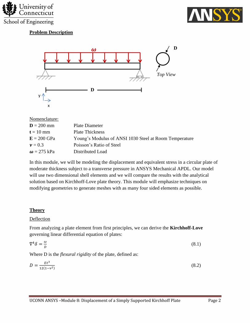
Theory

Deflection

From analyzing a plate element from first principles, we can derive the Kirchhoff-Love

governing linear differential equation of plates:

(8.1)

Where D is the flexural rigidity of the plate, defined as:

( ) (8.2)

x

y

𝝎 D

Top View

D


The flexural rigidity is a constant that is a result of the derivation of plate equilibrium. We can

draw comparisons to Euler-Bernoulli Beam theory where the governing relationship is:

( ) (8.3)

where EI is considered the flexural rigidity. The main difference between the two concepts is that

the 2D flexural rigidity takes into consideration multi-axial strains and thus incorporates

Poisson’s Ratio. Equation 8.1 was derived with a linear Taylor Series expansion of the internal

forces, moments, and angular distortions (twisting) on an individual stress element. Thus, this

model assumes small deflections and a certain ratio of plate thickness to plate radius. Most

sources recommend a radius to thickness ratio of at least 5:1, but not larger than 20:1. To get the

most accurate results, a proportion of 10:1 is recommended, which is what we have chosen for

our tutorial. In terms of “small deflections” the following table outlines potential error as a

function of deflection normalized by the plate’s thickness.

Deflection

(δ/t)

Percent Error

(%)

0.10 0.05

0.25 3

0.33 5

0.50 10

As one can see, any deflection greater than half of the thickness of the plate results in large

errors. For the purpose of this tutorial, we chose a deflection less than 10% the thickness of the

plate for greatest accuracy.

Since the loading we have chosen does not create any twisting effects in the plate and the load is

axis-symmetric, all of the

and

terms equal zero. Thus, equation 8.1 reduces to:

(

(

(

)))

(8.4a)

This is a separable equation. Solving for ( ), we can derive:

( )

( ) ( ) (8.4b)

Since we know ( ) is finite, this leaves us with

( )

(8.4c)

Now all we need are 2 boundary conditions to solve this problem. Since this is a simply

supported plate, we know that ( ) and that ( )


From plate theory, we can derive:

(

(

)) (8.5)

Since the

terms = 0 due to no twisting, the above equation only requires the first and second

derivative of ( ). Plugging those relationships and the boundary condition ( ) into

equation 8.5a, we get:

(8.6)

Plugging in and the other boundary condition into equation 8.4c, we get

(8.7)

Thus, the deflection in a simply supported Kirchhoff plate subject to transverse pressure is:

( )

(

) (8.8)

With maximum deflection ( ) 0.0956 mm which is less than 10% the thickness.

Equivalent Stress

Similar to bending in beams, the total stress in a plate without twisting is

( ) ( )

(8.9)

Where M is the moment-sum of the radial and angular bending moments. For our model,

( ) ( )

( ) (

)

= 34 MPa (8.10)

This is less than 10% of the yield strength of ANSI 1030, so we are in the elastic range of the

material.


Geometry

Preferences

1. Go to Main Menu -> Preferences

2. Check the box that says Structural

3. Click OK

1

2

3


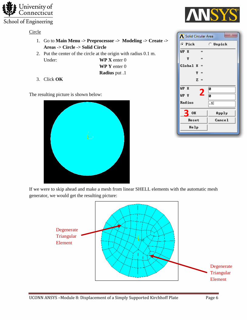
Circle

1. Go to Main Menu -> Preprocessor -> Modeling -> Create ->

Areas -> Circle -> Solid Circle

2. Put the center of the circle at the origin with radius 0.1 m.

Under: WP X enter 0

WP Y enter 0

Radius put .1

3. Click OK

The resulting picture is shown below:

If we were to skip ahead and make a mesh from linear SHELL elements with the automatic mesh

generator, we would get the resulting picture:

2

3

Degenerate

Triangular

Element

Degenerate

Triangular

Element


As one can see from the above picture, the automatic settings generate a mesh with two

degenerate triangular elements. Triangular elements are mostly used to fill gaps and provide

transition between large differences in mesh size or orientation. The problem with triangular

elements is that they are constant strain triangles (CST) while the typical hex elements have

strain functions that vary linearly between nodes. Since hex elements provide a higher order

accurate strain function, it generally takes a lot less of these elements to reach convergence. With

that in mind, we will modify our geometry in such a way that will allow us to mesh the circle

using purely hex elements. The technique we will use is called Multi-Zone Mapped Meshing,

where we will split the geometry into several sub-geometries allowing for greater control of local

mesh options.

Modifying the Geometry

In order to create our Multi-Zone Mesh, we need to split the existing geometry into several parts.

1. Go to Main Menu -> Preprocessor -> Modeling -> Delete ->

Areas Only

2. Click Pick All

3. Go to Utility Menu -> Plot -> Lines

4. Go to Utility Menu -> PlotCtrls -> Numbering… and select

LINE Line numbers and press OK

The resulting plot should look like the picture below:

2


In general, the Parent – Child relationships in ANSYS are as follows:

PARENT Keypoint

Line

Area

Volume

Element

CHILD Node

In order to modify a parent feature, all child features must be deleted.

5. Go to Utiility Menu -> Plot -> Keypoints -> Keypoints

6. Go to Main Menu -> Preprocessor -> Modeling -> Create ->

Keypoints -> On Working Plane

7. In the open field, put 0, 0.05 and press enter

8. Repeat step 7 for the following keypoints: 0.05,0

0,-0.05

-0.05,0

9. Press OK

10. Utility Menu -> PlotCtrls -> Numbering… and select

KP Keypoint numbers and press OK

The resulting plot is shown below:

WARNING: When you delete child features, the parent features still exist. If you want a

geometry to completely disappear, make sure you take the time to delete all parent features.

All the delete options can be found under Main Menu -> Preprocessor -> Modeling ->

Delete

7

9


11. Go to Main Menu -> Preprocessor –Modeling -> Create -> Lines -> Lines ->

Straight Line

12. In the field, enter 7,4 and press enter

13. Repeat step 12 for the following lines: 6,1

5,2

3,8

6,5

5,8

8,7

6,7

Instead of entering the start and end points of the lines, they can

be clicked in the graphics window as well.

14. Click OK

15. Click Utility Menu -> Plot -> Lines …

16. Go to Utility Menu -> PlotCtrls -> Numbering … and deselect

KP Keypoint numbers and press OK

The resulting picture should look as follows:

12 14


17. Go to Main Menu -> Preprocessor -> Modeling -> Create -> Areas -> Arbitrary ->

By Lines

Since we will be applying surface loads to our final set of areas, it is important to remember the

right hand rule in creating our sub-geometry areas. The Load Keys responsible for determining

direction of surface loads (see module 1.6) depend on the construction of the area. According to

the right hand rule, if our area is defined by lines selected in a counterclockwise manner, the

surface normal will point up. Thus, load key 2 in the future will apply loads to the top surface of

the area.

18. By either clicking the lines in the picture or entering them in

the List of Items select lines 4,6,12,5 in that order and click Apply

19. Repeat step 18 for the remaining lines: 3,5,11,8

2,8,10,7

1,7,9,6

10,11,12,9

20. Click OK

21. Go to Utility Menu -> Plot -> Areas

WARNING: It is very important that all of the areas are generated with the same surface

normal direction. If there is a disagreement in the positive direction of the surface normal

between areas, loading will push on some areas while pull on others. Incorrectly defining

loads will lead to wrong answers, so double check the surface normals of all the surfaces you

generate

18 20


The resulting picture is shown below.

22. To check surface normal conditions, in the Command Prompt, enter /normal,all,1 and

press enter. This command selects all areas and hides the areas whose surface normal are

facing the opposite direction from the viewing angle.

23. In the Command Prompt enter /replot and press enter to see the change. Seeing no

change, we know all of the surface normals are oriented correctly.

The other tale tell sign of mismatched areas will occur during meshing. Meshed areas with the

surface normal facing the screen will be in blue while those with the surface normal facing away

will be purple

USEFUL TIP: If an area was generated with the surface normal in the wrong direction, use

the command AREVERSE, Area Number, 0 to change the direction of the surface normal.

This command can only be used before surface loads are applied to the area, so make sure

to check the orientations of your areas first before loading

CORRECT INCORRECT


Preprocessor

Element Type

1. Go to Main Menu -> Preprocessor ->

Element Type -> Add/Edit/Delete

2. Click Add

3. Click Shell -> 4node 181 the elements

that we will be using are four node

elements with six degrees of freedom.

4. Click OK

5. For more information on SHELL 181,

click the Help button to open ANSYS

Help

6. Go to ANSYS 12.1 Help ->Search

Keyword Search ->type

‘SHELL181’ and press Enter

7. Go to Search Options ->SHELL181

the element description should

appear in the right portion of the

screen.

8. Click Close

9. Go to Utility Menu -> ANSYS

Toolbar -> SAVE_DB

\

2

3

4

5

6

7

8


Real Constants and Material Properties

Now we will add the thickness to our beam.


Real Constants -> Add/Edit/Delete

2. Click Add

3. Click OK

4. Under Real Constants for SHELL181 ->

Shell thickness at node I TK(I) enter .01

for the thickness

5. Click OK

6. Click Close

Now we must specify Youngs Modulus and Poisson’s Ratio

7. Go to Main Menu -> Material Props -> Material Models

8. Go to Material Model Number 1 -> Structural -> Linear -> Elastic -> Isotropic

2

3

6

8

11

4

5


9. Enter 200E9 for Youngs Modulus (EX) and .3 for Poisson’s Ratio (PRXY)

10. Click OK

11. out of Define Material Model

Behavior

12. Go to Utility Menu -> SAVE_DB

Meshing

1. Go to Main Menu -> Preprocessor -> Meshing -> Mesh Tool

2. Go to Size Controls: -> Global -> Set

3. Under NDIV enter 4. This function will divide all geometry edge

lengths into 4 equal segments

4. Press OK

5. Under Mesh Tool -> Mesh select Areas

6. Under Mesh Tool -> Shape: select Quad and Mapped

7. Click Mesh

8. Select Pick All in the new window

9. Click Close if the window disappears from sight, click

Raise Hidden which is located next to the

Command Prompt

9

10

2

3

4

5

6

7

9

8



As one can see, this mesh contains no triangular elements! This was achieved because each of

our sub geometries had 4 sides. Since this was a uniform mapped mesh, border elements mate

perfectly with border elements in adjacent mesh zones. If the edge sizing was not uniform (i. e.

NDIV A1 = 4 and NDIV A2 = 6), there would be triangular elements appearing in the mesh to

make the transition between mesh zones. An example of this is shown below:

Lastly, even though our domain has been split into 5 regions, they are all perfectly bonded,

resulting in one solid plate. This type of meshing strategy can be used elsewhere when quad

elements are desired but the geometry requires modification to achieve that.


Loads

Displacements

Now it is time to apply our boundary conditions. Thankfully, since all our boundary conditions

are surface conditions, we don’t have to reapply them when we re- mesh! Boundary conditions

only need to be reapplied for nodal constraints.

1. Go to Utility Menu -> Plot -> Lines

2. Go to Main Menu -> Preprocessor -> Loads -> Define Loads -> Apply ->

Structural -> Displacement -> On Lines

3. Under List of Items enter 1,2,3,4 and click Apply

4. In the new window, select Lab2 -> UX

5. Under Value put 0

6. Click Apply

7. Repeat steps 3-6 for the constraints UY, UZ, and ROTZ. We

constrain ROTZ to prevent any twisting.

8. Click OK


3

4

5

6

8


Uniform Pressure

1. Go to Main Menu -> Preprocessor -> Loads -> Define Loads -> Apply ->

Structural -> Pressure -> On Areas

2. Click Pick All

3. Under VALUE enter 275000

4. Under LKEY enter 2. This selects surface 2 (see page 10)

5. Click OK

2

3

4

5


1. To check the load orientation, go to Utility Menu -> Plot Ctrls -> Symbols …

2. Under Boundary condition symbol

Click All Applied BCs

3. Under Surface Load Symbols

select Pressures

4. Under Show pres and convect as

select Areas

5. Click OK

6. Go to Utility Menu -> Plot -> Areas

7. Click the Isometric View

Solve

The resulting picture should look like below:

The picture validates that the pressure is acting in the negative normal direction of each area.

Solution

1. Go to Main Menu -> Solution ->Solve -> Current LS (solve). LS stands for Load Step.

This step may take some time depending on mesh size and the speed of your computer

(generally a minute or less).

2

3

4

5


General Postprocessor

Deflection

1. Go to Main Menu -> General Postprocessor -> Plot Results -> Contour Plot -> Nodal

Solution -> DOF Solution ->X-Component of displacement -> OK

2. Select the Front View

The following graphic should appear:

According to the contour plot, the maximum displacement was 0.959E-4 meters in the –Z

Direction: not a bad initial answer considering the analytical solution (page 4). To make aesthetic

modifications to your contour plot, see module 1.4 page 16.


Von-Mises Equivalent Stress

1. Go to Main Menu -> General Postprocessor -> Plot Results -> Contour Plot -> Nodal

Solution -> Stress -> von Mises stress -> OK

The following graphic should appear:

According to the contour plot, the maximum Von-Mises Stress is 33.5 GPa not a bad initial

answer considering the analytical solution (page 4). To make aesthetic modifications to your

contour plot, see module 1.4 page 16.


Results

Max Deflection Error

The percent error (%E) in our model max deflection can be defined as:

(

) = 0.314% (8.11)

Our superior meshing job rewarded us with a coarsely meshed model with a near perfect

solution! This proves the advantages of using a Multi-Zone Mapped Mesh over a geometry

that, if otherwise meshed using automatic settings would produce less accurate results. For a

more detailed analysis, see the Validation section.

Max Equivalent Stress Error

Using the same definition of error as before, we derive that our model has 1.47% error in the

max equivalent stress. Using the NDIV20 finer mesh instead of NDIV4 results in a perfectly

converged solution.


Validation

Von-Mises Equivalent Stress

Global Number of Divisions (NDIV) ANSYS Max Stress (Pa) Percent Error (%)

4 3.35E+07 1.471

20 3.40E+07 0

40 3.40E+07 0

As one can see, the maximum stress converges to the theoretical value after setting NDIV to 20.

Since this module focuses on deflection, we did not compile results for the stress distribution

through the plate. According to plate theory, the Von-Mises stress is a function of and , both

of which are a function of r. For simplicity, we calculated at the coordinate where these two

values are equal, the center.

Deflection

As we can see in the above convergence plot, the ANSYS Solution converges to the theoretical

answer after NDIV20 (2000 elements). This is evident because the NDIV40 solution (8000

elements) matches up perfectly with the NDIV20 solution. The only slight variation occurs at

r = 0.05 due to errors in establishing the halfway point in the plate (this is where the diamond

area in the center intersects a boundary area.) Even though the quad elements in areas 1 through

4 are not perfectly rectangular, they are mapped the same way as the perfectly square elements.

-1.E-4

-1.E-4

-8.E-5

-6.E-5

-4.E-5

-2.E-5

0.E+0

0 0.02 0.04 0.06 0.08 0.1

De

fle

ctio

n(m

)

Radial Distance (m)

Deflection vs Radial Distance From Center Theoreti

cal

NDIV4


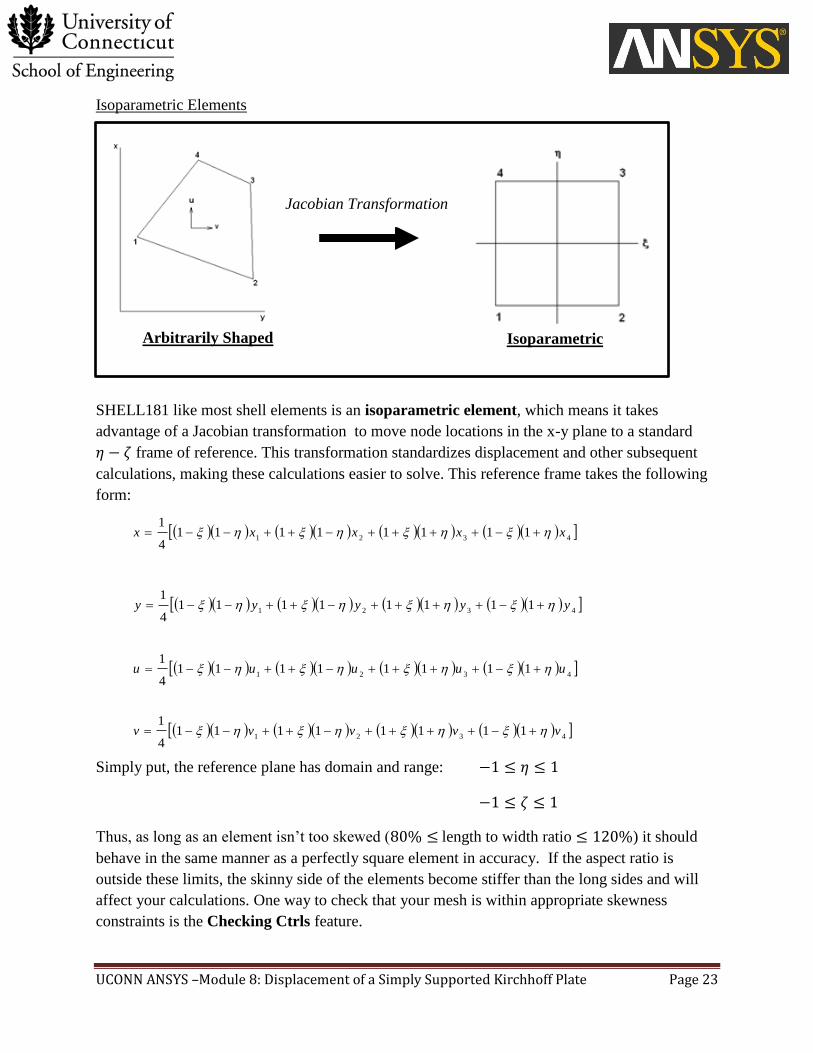
Isoparametric Elements

SHELL181 like most shell elements is an isoparametric element, which means it takes

advantage of a Jacobian transformation to move node locations in the x-y plane to a standard

frame of reference. This transformation standardizes displacement and other subsequent

calculations, making these calculations easier to solve. This reference frame takes the following

form:

Simply put, the reference plane has domain and range:

Thus, as long as an element isn’t too skewed ( length to width ratio ) it should

behave in the same manner as a perfectly square element in accuracy. If the aspect ratio is

outside these limits, the skinny side of the elements become stiffer than the long sides and will

affect your calculations. One way to check that your mesh is within appropriate skewness

constraints is the Checking Ctrls feature.

Arbitrarily Shaped Isoparametric

Jacobian Transformation

4321

111111114

1xxxxx

4321

111111114

1yyyyy

4321

111111114

1uuuuu

4321

111111114

1vvvvv


Checking Ctrls

For the NDIV4 model we built in this tutorial, let’s check the skewness of our elements.


Checking Ctrls -> Shape Checking

2. Select Summary

3. Click OK

The following table should populate:

Since the shape checking produced no errors or warning, our mesh meets the ANSYS skewness

criteria for elements.

2

3

Documents

Module 8: Displacement of a Simply Supported Kirchhoff Plate