Embed Size (px)
Citation preview
University of Central Florida University of Central Florida
STARS STARS
Electronic Theses and Dissertations, 2004-2019
2009
Molecular Dynamics Study Of Thermal Conductivity Enhancement Molecular Dynamics Study Of Thermal Conductivity Enhancement
Of Water Based Nanofluids Of Water Based Nanofluids
Parveen Sachdeva University of Central Florida
Part of the Mechanical Engineering Commons
Find similar works at: https://stars.library.ucf.edu/etd
University of Central Florida Libraries http://library.ucf.edu
This Doctoral Dissertation (Open Access) is brought to you for free and open access by STARS. It has been accepted
for inclusion in Electronic Theses and Dissertations, 2004-2019 by an authorized administrator of STARS. For more
information, please contact [email protected].
STARS Citation STARS Citation Sachdeva, Parveen, "Molecular Dynamics Study Of Thermal Conductivity Enhancement Of Water Based Nanofluids" (2009). Electronic Theses and Dissertations, 2004-2019. 3935. https://stars.library.ucf.edu/etd/3935
MOLECULAR DYNAMICS STUDY OF THERMAL CONDUCTIVITY ENHANCEMENT OF WATER BASED NANOFLUIDS
by
PARVEEN SACHDEVA B.Tech. Indian Institute of Technology Kanpur, 2003
M.S. University of Central Florida, 2006
A dissertation submitted in partial fulfillment of the requirements for the degree of Doctor of Philosophy
in the Department of Mechanical, Materials and Aerospace Engineering in the College of Engineering and Computer Science
at the University of Central Florida Orlando, Florida
Fall Term 2009
Major Professor: Ranganathan Kumar

© 2009 Parveen Sachdeva
ii

ABSTRACT
A systematic investigation using molecular dynamics (MD) simulation involving
particle volume fraction, size, wettability and system temperature is performed and the
effect of these parameters on the thermal conductivity of water based nanofluids is
discussed. Nanofluids are a colloidal suspension of 10 -100 nm particles in base fluid. In
the last decade, significant research has been done in nanofluids, and thermal
conductivity increases in double digits were reported in the literature. This anomalous
increase in thermal conductivity cannot be explained by classical theories like Maxwell’s
model and Hamilton-Crosser model for nanoparticle suspensions. Various mechanisms
responsible for thermal conductivity enhancement in nanofluids have been proposed and
later refuted. MD simulation allows one to predict the static and dynamic properties of
solids and liquids, and observe the interactions between solid and liquid atoms.
In this work MD simulation is used to calculate the thermal conductivity of water
based nanofluid and explore possible mechanisms causing the enhancement. While most
recent MD simulations have considered Lennard Jones (LJ) potential to model water
molecule interactions, this work uses a flexible bipolar water molecule using the Flexible
3 Center (F3C) model. This model maintains the tetrahedral structure of the water
molecule and allows the bond bending and bond stretching modes, thereby tracking the
motion and interactions between real water molecules. The choice of the potential for
solid nanoparticle reflects the need for economic but insightful analyses and reasonable
accuracy. A simple two body LJ potential is used to model the solid nanoparticle. The
iii
cross interaction between the solid and liquid atoms is also modeled by LJ potential and
the Lorentz-Berthelot mixing rule is used to calculate the potential parameters.
The various atomic interactions show that there exist two regimes of thermal
conductivity enhancement. It is also found that increasing particle size and decreasing
particle wettability cause lower thermal conductivity enhancement. In contrast to the
previous studies, it is observed that increasing system temperature does not enhance
thermal conductivity significantly. Such enhancement with temperature is proportional to
the conductivity enhancement of base fluid with temperature. This study demonstrates
that the major cause of thermal conductivity enhancement is the formation of ordered
liquid layer at the solid-liquid interface. The enhanced motion of the liquid molecules in
the presence of solid particles is captured by comparing the mean square displacement
(MSD) of liquid molecules in the nanofluid to that of the base fluid molecules. The
thermal conductivity is decomposed into three modes that make up the microscopic heat
flux vector, namely kinetic, potential and collision modes. It was observed by this
decomposition analyses that most of the thermal conductivity enhancement is obtained
from the collision mode and not from either the kinetic or potential mode. This finding
also supports the observation made by comparing the MSD of liquid molecules with the
base fluid that the interaction between solid and liquid molecules is important for the
enhancement in thermal transport properties in nanofluids.
These findings are important for the future research in nanofluids, because they
suggest that if smaller, functional nanoparticles which have higher wettability compared
to the base fluid can be produced, they will provide higher thermal conductivity
compared to the regular nanoparticles.
iv
Dedicated to my mother Mrs. Asha Sachdeva & Nirankari Baba Hardev Singh Ji
v
ACKNOWLEDGMENTS
This work and my stay at UCF has been a great learning experience for me. I
would like to take this opportunity to express gratitude to my advisor Dr. R. Kumar for
his constant support, advice and guidance throughout my stay at UCF. It was a rewarding
experience working with him. I also acknowledge and offer thanks to my committee
members Dr. J. Kapat, Dr. Q. Chen, Dr. S. Basu and Dr. A. Masunov for their valuable
comments and guidance. I also acknowledge the support of the College of Engineering &
Computer Science and the I2Lab at the University of Central Florida for the research
presented here.
I would also like to thank my friends at UCF for making my stay memorable. I
thank the UCF Indian student association, Sangam for their help when I first came to
USA.
None of this would have been possible without the blessings of Nirankari Baba
Hardev Singh Ji and the constant support and encouragement of my family members.
vi
TABLE OF CONTENTS
LIST OF FIGURES ............................................................................................................ x
LIST OF TABLES............................................................................................................ xii
CHAPTER ONE: INTRODUCTION................................................................................. 1
1.1 Colloids ..................................................................................................................... 5
1.2 Nanofluids................................................................................................................. 6
1.2.1 Benefits of Nanofluids ....................................................................................... 7
1.3 Problem Description ............................................................................................... 11
CHAPTER TWO: LITERATURE REVIEW................................................................... 14
2.1 Experimental Results for Nanofluids...................................................................... 14
2.1.1 Effect of Particle Volume Fraction .................................................................. 23
2.1.2 Effect of Particle Size ...................................................................................... 27
2.1.3 Effect of System Temperature ......................................................................... 29
2.2 Modeling of Nanofluids.......................................................................................... 32
2.3 Computer Simulations of Nanofluids ..................................................................... 36
2.4 Literature Review on Molecular Dynamics Simulation ......................................... 43
2.4.1 Thermal Conductivity Calculation using Molecular Dynamics Simulation.... 44
CHAPTER THREE: METHODOLOGY ......................................................................... 50
3.1 Molecular Dynamics Simulation ............................................................................ 54
3.1.1 Potential Functions........................................................................................... 56
3.1.2 Force Calculation ............................................................................................. 59
3.1.3 Cut-off Radius.................................................................................................. 59
vii

3.1.4 Verlet Neighbor List ........................................................................................ 60
3.1.5 Integration of Equation of Motion ................................................................... 62
3.1.6 Periodic Boundary Condition .......................................................................... 64
3.2 Molecular Simulation of Liquid Water................................................................... 65
3.3 Potential Functions Used in This Work .................................................................. 68
3.3.1 Liquid-Liquid Interaction................................................................................. 68
3.3.2 Interactions in Solid Nanoparticle ................................................................... 72
3.3.3 Interaction between Solid-Liquid Atoms......................................................... 73
3.3.4 Coulombic Interaction ..................................................................................... 76
3.3 Generation of Nanoparticle..................................................................................... 79
3.4 Molecular dynamics simulation of Thermal Conductivity ..................................... 81
CHAPTER FOUR: VALIDATION OF THE MD CODE ............................................... 84
4.1 Validation of Lennard-Jones based MD code......................................................... 84
4.1 Validation of F3C water model............................................................................... 91
CHAPTER FIVE: RESULTS & DISCUSSION .............................................................. 98
5.1. Effect of Particle Volume Fraction ...................................................................... 101
5.2. Effect of Particle Size .......................................................................................... 110
5.3. Effect of System Temperature ............................................................................. 113
5.4. Effect of Particle Wettability ............................................................................... 117
5.5. Possible Mechanisms Enhancing Thermal Conductivity in Nanofluids.............. 121
5.5.1. Hydration Layer Formation at the Solid-Liquid Interface............................ 121
5.5.2. Mean Square Displacement (MSD) .............................................................. 127
5.5.3. Diffusion Coefficient .................................................................................... 131
viii
5.5.4. Heat Current Autocorrelation Function (HCAF) Decomposition ................ 135
5.5.5. Strong Particle-Fluid Interaction................................................................... 138
CHAPTER SIX: SUMMARY & FUTURE WORK ...................................................... 140
1.1 Future Work .......................................................................................................... 143
LIST OF REFERENCES................................................................................................ 145
ix
LIST OF FIGURES
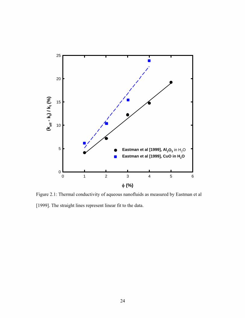
Figure 2.1: Thermal conductivity of aqueous nanofluids as measured by Eastman et al
[2003]. The straight lines represent linear fit to the data. ................................................. 24
Figure 2.2: Relative thermal conductivity of oil-MWCNT suspension as measured by
Choi et al [2001], showing the quadratic relationship between conductivity and volume
fraction. In the inset, line A represents the Hamilton-Crosser model and B represents the
Maxwell’s model .............................................................................................................. 25
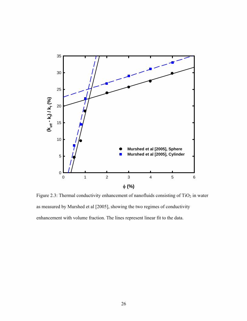
Figure 2.3: Thermal conductivity enhancement of nanofluids consisting of TiO2 in water
as measured by Murshed et al [2005], showing the two regimes of conductivity
enhancement with volume fraction. The lines represent linear fit to the data. ................. 26
Figure 2.4: Thermal conductivity enhancement of nanofluids as a function of particle
size, as measured by various groups ................................................................................. 28
Figure 2.5: Thermal conductivity enhancement of nanofluids as a function of temperature
as measured by various groups ......................................................................................... 31
Figure 2.6: Schematic of the simulation domain used in NEMD simulation by Wu &
Kumar [2004].................................................................................................................... 46
Figure 3.1: Simulation techniques for various length and time scales [Smith G., 1999] . 51
Figure 3.2: General flowchart of molecular dynamics simulation algorithm................... 55
Figure 3.3: Potential energy of a particle in LJ model...................................................... 58
Figure 3.4: Neighbor-list construction with radius rlist ..................................................... 61
Figure 3.5: Structure of water molecule ........................................................................... 66
Figure 4.1: Face centered cubic (FCC) unit cell structure ................................................ 86
Figure 4.2: Initial system configuration for a 256 atoms Argon system .......................... 87
x
Figure 4.3: Thermal conductivity of the liquid argon at T* = 0.73 and ρ* = 0.8442....... 89
Figure 4.5: Thermal conductivity of water with varying simulation domain size............ 93
Figure 4.6: Thermal conductivity of water vs. the Green-Kubo correlation length ......... 96
Figure 5.1: (a) Initial configuration of a 1 nm nanofluid at 1.8% volume concentration,
(b) Nanofluid system with periodic boundary condition applied in x and y planes ....... 100
Figure 5.2: Thermal conductivity vs. volume concentration for 1 nm particle .............. 104
Figure 5.3: Thermal conductivity vs. volume concentration for 2 nm particle .............. 105
Figure 5.4: Thermal conductivity vs. particle size.......................................................... 111
Figure 5.5: Thermal conductivity vs. system temperature.............................................. 115
Figure 5.6 Thermal conductivity vs. particle wettability (increasing “c” means higher
wettability) ...................................................................................................................... 119
Figure 5.7 Spherical shells around the solid nanoparticle (NP) to plot density distribution
[Teng et al, 2008]............................................................................................................ 125
Figure 5.8: Relative number density distribution around the nanoparticle as a function of
distance from the nanoparticle surface ........................................................................... 126
Figure 5.9: Mean square displacement at various volume concentrations for 1 nm
nanofluid ......................................................................................................................... 129
Figure 5.10: Relative diffusion coefficient at various concentrations for 1 nm nanofluid
......................................................................................................................................... 133
Figure 5.11: Thermal conductivity contribution by various heat current modes............ 137
xi
xii
LIST OF TABLES
Table 1: Thermal conductivities of various materials at room temperature ....................... 4
Table 2.1: Experimental investigation of nanofluid thermal conductivity ....................... 15
Table 2.2: Molecular dynamics simulation studies of nanofluid (*SS, LL, SL refer to
solid-solid, liquid-liquid, and solid-liquid respectively)................................................... 37
Table 4.1: Thermal conductivity of liquid argon with varying system size ..................... 90
Table 4.2: Thermal conductivity of water with varying system size................................ 94
Table 5.1: Volume concentration of various cases considered for 1 nm nanoparticle ... 106
Table 5.2: Thermal conductivity of various cases considered for 1 nm nanoparticle .... 107
Table 5.3: Thermal conductivity of various cases considered for 2 nm nanoparticle .... 108
Table 5.4: Thermal conductivity for variable particle size at 5.1% volume concentration
......................................................................................................................................... 112
Table 5.5: Thermal conductivity at various system temperatures for 1 nm particle case116
Table 5.6: Thermal conductivity of nanofluid with varying wettability (increasing “c”
means higher wettability)................................................................................................ 120
Table 5.7: Diffusion coefficient at various concentrations for 1 nm nanofluid.............. 134
CHAPTER ONE: INTRODUCTION
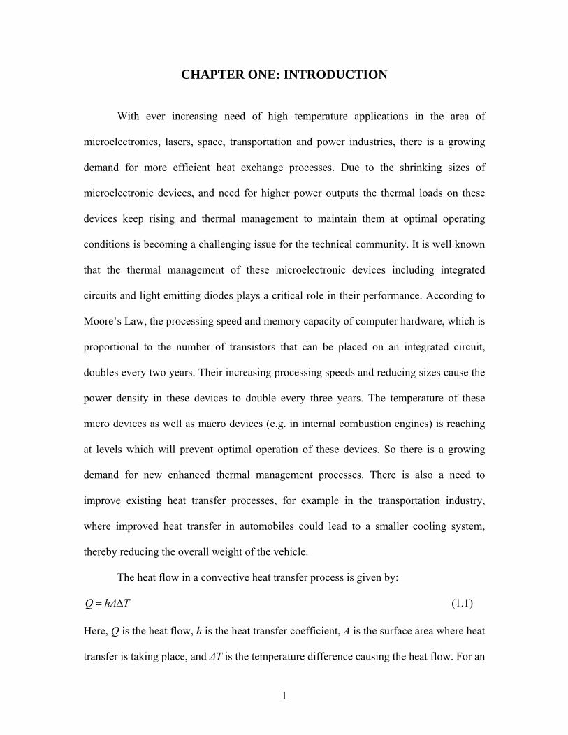
With ever increasing need of high temperature applications in the area of
microelectronics, lasers, space, transportation and power industries, there is a growing
demand for more efficient heat exchange processes. Due to the shrinking sizes of
microelectronic devices, and need for higher power outputs the thermal loads on these
devices keep rising and thermal management to maintain them at optimal operating
conditions is becoming a challenging issue for the technical community. It is well known
that the thermal management of these microelectronic devices including integrated
circuits and light emitting diodes plays a critical role in their performance. According to
Moore’s Law, the processing speed and memory capacity of computer hardware, which is
proportional to the number of transistors that can be placed on an integrated circuit,
doubles every two years. Their increasing processing speeds and reducing sizes cause the
power density in these devices to double every three years. The temperature of these
micro devices as well as macro devices (e.g. in internal combustion engines) is reaching
at levels which will prevent optimal operation of these devices. So there is a growing
demand for new enhanced thermal management processes. There is also a need to
improve existing heat transfer processes, for example in the transportation industry,
where improved heat transfer in automobiles could lead to a smaller cooling system,
thereby reducing the overall weight of the vehicle.
The heat flow in a convective heat transfer process is given by:
Q hA T= Δ (1.1)
Here, Q is the heat flow, h is the heat transfer coefficient, A is the surface area where heat
transfer is taking place, and ΔT is the temperature difference causing the heat flow. For an
1
efficient thermal management system, we would like to increase the heat flow from the
device. As seen from equation (1.1) the heat flow increase can be achieved by: (1)
increasing ΔT, (2) increasing A, or (3) increasing h.
Increasing the temperature difference between the cooling fluid and the device
can lead to higher heat flow, but often these two temperature limits are set by
environmental and material constraints. The temperature of the cooling fluid is often set
at atmospheric conditions, and the device temperature is governed by the maximum
temperature the material can take, for example in a power generation turbine, the highest
temperature is decided by the blade material used in the first stage of the turbine.
Increasing ΔT to enhance the heat flow is not an easy option, as in most processes these
two temperatures have already been taken to their limits.
Another method to increase heat transfer rates in any application is to increase the
heat transfer surface area, A. Conventionally the surface area is increased by using
extended surfaces, such as fins, which exchange heat with the heat transfer fluid.
Unfortunately, this method to increase heat transfer requires an increase in the size of the
thermal management system. However, when dealing with microelectronic devices or
high speed lasers, the surface area can not be increased at will. Increasing the surface area
would mean a larger and heavier device, which is essentially going against the trend of
reducing the size of devices.
The last method to improve the heat flow in an application is to increase the heat
transfer coefficient, h. The heat transfer coefficient depends on the heat transfer process
used, and on the properties of the heat transfer fluid, for example the heat transfer
coefficient is higher for forced convection compared to natural convection, and it is also
2
higher for a turbulent flow compared to laminar flow. Since most of these thermal
management processes already use forced convection heat transfer, the alternative to
increase h, is to improve the thermal properties of the heat transfer fluid. Water, ethylene
glycol and engine oil are the most common heat transfer fluids used in most industrial
applications, like transportation, space applications, manufacturing and even
microelectronics. Heat transport characteristics of these fluids are vital in designing and
developing high efficiency heat transfer equipments. Unfortunately, these fluids have
very low thermal conductivity (less than 1.0 Wm-1˚K-1), so the inherently poor
thermophysical properties of these cooling fluids greatly limit the performance of thermal
management systems. Thermal conductivity of these fluids plays an important role in the
development of thermal management systems. Low thermal conductivity of these fluids
hinders high effectiveness and compactness of heat exchangers and other devices.
Additives are often added to heat transfer fluids, to improve their thermophysical
properties, for example in automobiles, glycols (alcohols) are often added to water as
antifreeze, to reduce its freezing point. Solids can also be added to the heat transfer fluids
to enhance their thermophysical properties. As shown in Table 1.1 solids (metals, non-
metals) have several orders of magnitude higher thermal conductivity compared to
liquids. It can be seen that the thermal conductivity of copper is about 650 times greater
than that of water, about 1500 times greater than that of ethylene glycol and about 3000
times that of engine oil. Therefore, it would be expected that adding these metallic or
non-metallic solid particles would significantly enhance the thermophysical properties of
conventional heat transfer fluids.
3
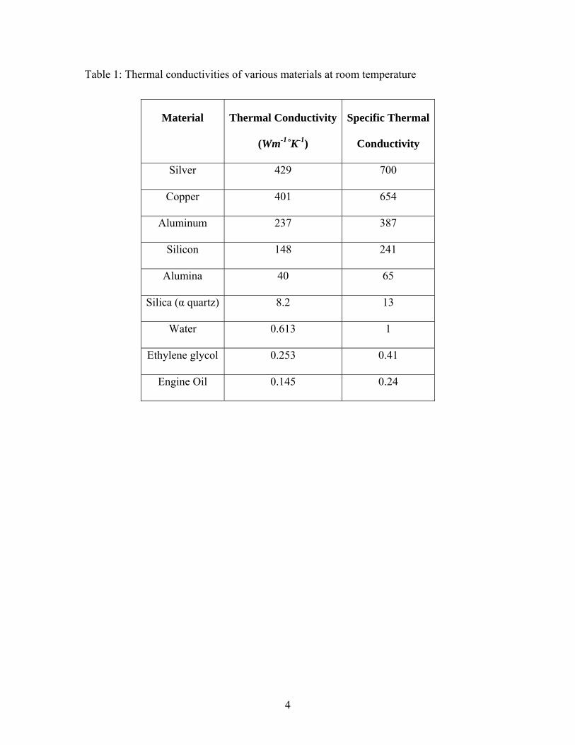
Table 1: Thermal conductivities of various materials at room temperature
Material Thermal Conductivity
(Wm-1˚K-1)
Specific Thermal
Conductivity
Silver 429 700
Copper 401 654
Aluminum 237 387
Silicon 148 241
Alumina 40 65
Silica (α quartz) 8.2 13
Water 0.613 1
Ethylene glycol 0.253 0.41
Engine Oil 0.145 0.24
4
1.1 Colloids
Numerous theoretical and experimental studies on increasing the thermal
conductivity of liquids by suspending solid particles have been performed in the past.
Earlier studies on thermal conductivity measurement of solid-liquid colloidal suspensions
were confined to millimeter and micrometer size particles. Ahuja [1975] studied
suspension of micron size polystyrene particles suspended in ethylene glycol and
observed that the heat transfer was increased by a factor of 3 under laminar flow
conditions for particle volume fraction of up to 9%. No significant pressure drop was
observed even for these high particle volume concentrations. Liu et al [1988] also found
enhanced heat transfer in micron size particulate slurries.
Even with these promising high heat transfer rates and low rise in pressure drop
by adding micron size particles to liquids, these suspensions were not used in any
industrial application because of some problems associated with them. A major drawback
of micron sized particles used in theses suspensions is that due to their weight, they tend
to settle down quickly. The rapid settling of solid particles in flow situation can cause
clogging of pipe or channel, resulting in high pressure drops. If the fluid is kept
circulating to prevent settling of solid particles, these large particles can cause erosion to
the channel walls. So the advantage of enhanced heat transfer in solid-liquid suspensions
is hindered by the erosion and high pressure drop caused by particle settling. Even though
the suspensions of these particles have higher thermal conductivity compared to their
base fluids, they have little application in engineering systems due to above mentioned
problems.
5
1.2 Nanofluids
With the advent of nanotechnology it has become possible to manufacture nano-
sized particles from metals, oxides and carbides. Researchers have been able to
manufacture nanometer sized particles using both, chemical and vapor deposition
techniques. The most common method for the preparation of semiconductor
nanoparticles is the synthesis from the starting reagents in solution by arresting the
reaction at a definite moment of time. This is the so-called method of arrested
precipitation. It is also possible to obtain semiconductor nanoparticles by sonication of
colloidal solutions of large particles. The gas phase synthesis could also be used to
manufacture nanoparticles. One method for the gas-phase synthesis of nanoparticles of
various materials is based on the pulsed laser vaporization of metals in a chamber filled
with a known amount of a reagent gas followed by controlled condensation of
nanoparticles onto the support.
Nanofluids are a new class of solid-liquid suspensions which offer a promise in
the development of energy-efficient heat transfer fluids. Application of solid
nanoparticles provides an effective way of increasing thermal conductivity of fluids.
Nanofluids are colloidal suspensions of metal or oxide particles, 1-100 nm in size,
suspended in base fluids like water, ethylene glycol or oil. Nanofluids could positively
impact the performance of heat exchangers or cooling devices, which are vital in many
industries. For example the automotive and aerospace industry has been trying to reduce
the weight of the thermal management systems to reduce the overall weight of the
vehicle.
6
1.2.1 Benefits of Nanofluids
Nanofluids could increase the heat transfer in various applications involving
coolants and lubricants and help reduce the system size and weight, which would also
enhance the overall efficiency of the process. Due to their ultra small sizes, these
nanoparticles have very high surface area to volume ratio and also high mobility. When
these nanoparticles are properly dispersed in base fluid, they are expected to offer
following benefits:
1) Enhanced heat transfer - As seen from equation (1.1) the surface area at
which heat transfer takes place is important in governing the overall
heat flow rate. So the nanoparticle which have surface area to volume
ratio much larger compared to microparticles, provide significantly
more heat transfer at same volume fractions. Additionally, particles
smaller than 20 nm have more than 20% of atoms on their surface
[Choi et al 2004] making them instantaneously available for thermal
interaction with fluid molecules. Due to their ultrafine size, these
nanoparticles show high mobility and can flow even through tiny
microchannels. These ultrafine nanoparticles flow with the base fluid
and can increase the dispersion of heat in the fluid at faster rate.
2) Stability – Again due to their small size, these particles weigh very less
compared to microparticles. So gravity becomes less important in case
of nanoparticles and chances of sedimentation of these particles in the
suspension are very less. If proper chemical conditioning, e.g.
dispersant, is used these nanoparticles can remain suspended in the base
7
fluid for weeks. This reduced settling of nanoparticles can overcome a
major drawback because of which suspensions of microparticles were
not used in many applications. The reduced sedimentation of
nanoparticles makes them more stable.
3) No clogging – Microchannels are used for cooling of MEMS devices
and biotech devices like “lab on a chip”. Due to their small sizes these
nanoparticles can also be used in microchannel cooling applications.
The combination of small nanoparticles with microchannel will provide
for very high heat transfer surface area and due to their small size, these
nanoparticles will not clog the small channels.
4) Reduced erosion of channel walls – One other drawback of
microparticles was that due to their larger size, they could wear the
channel or pipe walls in which the microparticle-fluid suspension was
flowing. But nanoparticles with their negligible mass would impart
very less momentum to the channel wall and reduce the chances of
erosion.
5) Reduction in pumping power requirement – In a forced convection heat
transfer process a ten fold increase in the pumping power is required to
increase the heat transfer rate by a factor of two. Since the heat transfer
rate is proportional to the thermal conduction of the fluid, if fluid
thermal conductivity is increased by using nanoparticle suspensions,
required increase in pumping power will be very less, unless the
addition of nanoparticle causes sharp rise in fluid viscosity.
8
With all these benefits expected of nanofluids, the scientific community termed
them as “next generation of heat transfer fluids” and significant research has undergone
in measuring thermal transport properties of nanofluids. It has been shown that the
nanofluids show these unique features:
1) Stability – It was expected that due to their small size the nanoparticle
would not settle in the suspension for days. Nanofluids have been
shown to be stable for over a month when proper dispersing agents
were used [Lee et al 1999].
2) Small concentration requirement – Thermal conductivity increase of
over 40% was observed at a mere 0.3% volume concentration of copper
nanoparticles in ethylene glycol [Eastman et al 2001]. As discussed
later in chapter 2, similar large increases in thermal conductivity have
been observed for other nanofluids at very small nanoparticle volume
concentration.
3) Anomalous increase in thermal conductivity – 160% increase in the
thermal conductivity was observed when 1% multi-wall-carbon-
nanotubes (MWCNT) were suspended in engine oil [Choi et al 2001].
As discussed later in chapter 2, other studies have also shown such
anomalous increase in thermal conductivity of various nanofluids.
4) Particle size dependence – Early experiments with millimeter and
micrometer size particles showed that the thermal conductivity increase
depended only on the particle volume concentration, but in case of
nanofluids, different thermal conductivity enhancements were observed
9
at same particle volume fraction [Masuda et al 1993, Lee et al 1999].
The difference in two cases was the size of the Al2O3 nanoparticles
used. So for nanofluids, not only the particle concentration, but also the
particle size affects the thermal conductivity enhancement.
5) Temperature dependence – In early experiments significantly higher
enhancement in thermal conductivity of nanofluids was observed with
increasing system temperature from 20 ˚C to 50 ˚C [Das et al 2003].
This is exciting as this could mean potential for use of nanofluids in
many high temperature applications.
With these exciting benefits it is important to thoroughly study and understand
various mechanisms causing these unique features in nanofluids. As discussed later in
chapter 2, significant experimental and theoretical research has been conducted in the
area of nanofluids in last decade, but till date no consensus has been reached on the
possible mechanisms causing the thermal enhancement in nanofluids. The nanofluids
experiments conducted by one group have not yet been reproduced by other groups. The
anomalous increase in thermal conductivity of nanofluids could not be explained by
classical theories like Maxwell’s model [1881] and Hamilton-Crosser model [1962] for
suspensions consisting of well dispersed particles. The inability of these models to
predict the thermal conductivity enhancement of nanofluids was ascribed to the fact that
they did not take important parameters like particle size, shape, system temperature,
interaction between large number of surface atoms with fluid molecules, and modes of
thermal transport at nanoscale into account.
10
Keblinski et al [2002] attribute the enhancement in thermal conductivity to four
possible mechanisms, (1) Brownian motion of particles, (2) layering of liquid molecules
around the particles, (3) ballistic nature of heat transport in nano-structures, and (4)
nanoparticle clustering. Various other mechanisms including (a) collision between base
fluid molecules, (b) thermal diffusion in nanoparticles in fluid, (c) collision between
nanoparticles due to Brownian motion, (d) thermal interaction between nanoparticle and
base fluid molecules [Jang & Choi 2004, Prasher et al 2005, Ren et al 2005] have been
proposed. Particles move through liquid by Brownian motion and collide with each other,
hence enabling direct solid-solid transport of heat from one to another. Some of these
mechanisms have been later refuted [Gupta et al 2007, Eapen et al 2007], even by the
groups that originally proposed them [Keblinski et al 2008]. Possible reason for all this is
disconnect between experimental and theoretical understanding of thermal transport
mechanisms at nanoscale. With macroscale experiments we can only measure thermal
transport properties of nanofluids, but we can not explore the mechanisms causing the
enhancement at the nanoscale.
1.3 Problem Description
A systematic study using computer simulation is required to determine the cause
of thermal conductivity enhancement in nanofluids and to explore possible mechanisms
at nanoscale. Due to the length and time scales involved in nanofluids, conventional
macroscale computational techniques such as CFD and FEM can not be used to capture
the properties. Molecular dynamics (MD) simulation, an atomic scale simulation
technique has been proven to predict the static and dynamic properties of solids and
11
liquids. In this work, molecular dynamics simulation is used to calculate the thermal
conductivity of water based nanofluids and study possible mechanisms contributing to
significantly higher conductivity than proposed by traditional models such as Hamilton
Crosser. Using MD, it is possible to observe the interactions between solid and liquid
atoms occurring at the molecular level, which give rise to the macroscale transport
properties. Accuracy of an MD model to simulate complex fluids such as nanoparticle
suspensions depends on the potential functions used to model the interaction between
various atoms in the system. Previous studies involving molecular dynamics simulation
of nanofluids have considered simplistic Lennard-Jones (LJ) potential to model the
interactions between both solid and liquid atoms [Keblinski et al 2002, Eapen et al 2007,
Sarkar & Selvam 2007, Li et al 2008]. In this work liquid water is modeled as a flexible
bipolar molecule using the Flexible 3 Center (F3C) model proposed by Levitt et al
[1997]. This model maintains the tetrahedral structure of the water molecule and allows
the H-O-H bond bending and O-H bond stretching modes, thereby mimicking the motion
and interactions between real water molecules.
The choice of the potential for solid nanoparticle in this work reflects the need for
economic but insightful analysis with reasonable accuracy. Since the complex surface
chemical reactions between the solid nanoparticle and fluid atoms have not yet been
identified by experiments, expensive quantum-chemistry based simulations would be
required to identify them. In this work, a simple two body Lennard-Jones potential is
used to model the solid nanoparticle. In addition, each atom in the nanoparticle is
connected to its first neighbors by finite extensible nonlinear elastic (FENE) bonding
potential [Vladkov & Barrat, 2006]. The atoms in this solid particle vibrate around their
12
mean position and simulate the phonon mode of heat transport as seen in solids. This
model nanoparticle will closely simulate a non-metallic particle like oxides, where the
thermal conductivity arises from the phonon mode and not from electrons as in the case
of metals. The cross interaction between solid and liquid atoms is modeled by the
Lennard-Jones potential and the Lorentz-Berthelot mixing rule [Allen & Tildesley, 1987]
is used to calculate the potential parameters. Linear response theory is combined with the
molecular dynamics simulation to calculate the thermal conductivity of the nanofluid
system. A systematic investigation involving particle volume fraction, size, wettability
and system temperature is undertaken using molecular dynamics simulation and the
effect of these parameters on the thermal conductivity of nanofluids is studied.
The focus of this thesis is to study the possible mechanisms causing the enhanced
thermal transport in nanofluids. The interaction between the solid and liquid atoms is
examined by tracking the motion of these molecules. The study of these mechanisms is
important as controversy still exists relating to the existence and nature of these
mechanisms, and their role in enhancing the heat transfer characteristics in colloidal
suspensions. The understanding of these mechanisms can help with the design of
engineering devices that use these nanofluids as heat transfer fluids. In this dissertation,
possible modes of thermal conduction in nanofluids are studied by decomposing the
microscopic heat flux vector in to three modes, namely kinetic, potential and collision.
Such a study of thermal transport in nanofluids would allow a practical engineer to
engineer the nanofluids by understanding the nature and behavior of nanoparticles in the
base fluids. The intellectual merit of this study is to understand the influence of the
various atomic potentials in the different modes of heat transfer is immeasurable.
13
CHAPTER TWO: LITERATURE REVIEW
Increasing the thermal transport properties of liquids by mixing high conductivity
solid particles is not a novel concept. As mentioned in chapter 1, Ahuja [1975] studied
colloidal suspension of micron-size polystyrene particles in ethylene glycol. He observed
heat transfer enhancement by a factor of 3 under laminar conditions at 9% particle
volume fraction. Liu et al [1988] carried out turbulent pipe flow experiments using
slurries containing micron sized high density polyethylene particles. They conducted
experiments to study the effect of particle volume fraction, particle size and flow rate on
the slurry pressure drop and heat transfer. They observed higher heat transfer in laminar
and turbulent flow conditions using these particulate slurries.
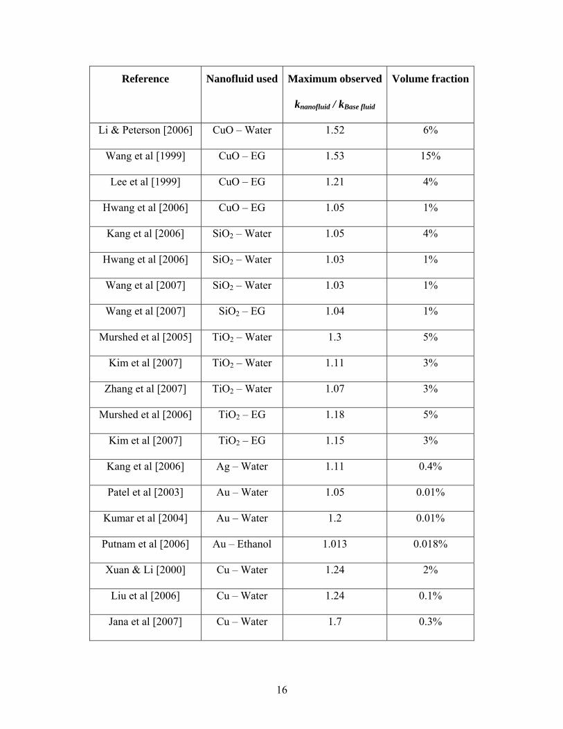
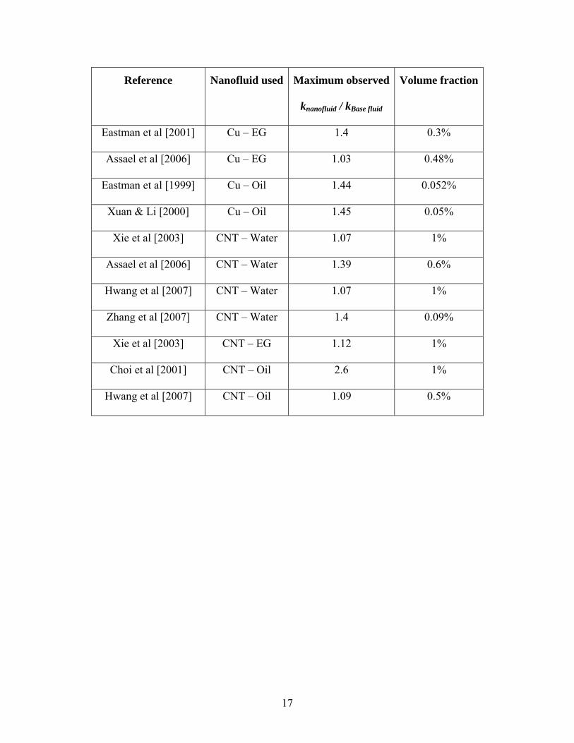
2.1 Experimental Results for Nanofluids
Significant research work has been conducted in the past decade to measure
thermal conductivity of nanofluids. Researchers have conducted experiments on
nanofluids containing various types of nanoparticles (Ag, Au, Cu, Al2O3, CuO, SiO2,
TiO2, CNT etc) dispersed in various base fluids (ethanol, ethylene glycol, oil, water,
toluene etc). Nanoparticles of sizes ranging from 10 nm to 250 nm in diameter have been
used in these studies. Researchers have looked at the effect of particle volume fraction,
size and system temperature on the thermal conductivity of nanofluid. Table 2.1 gives a
summary of experimental research work conducted in the last decade to measure thermal
conductivity of nanofluids at room temperature.
14
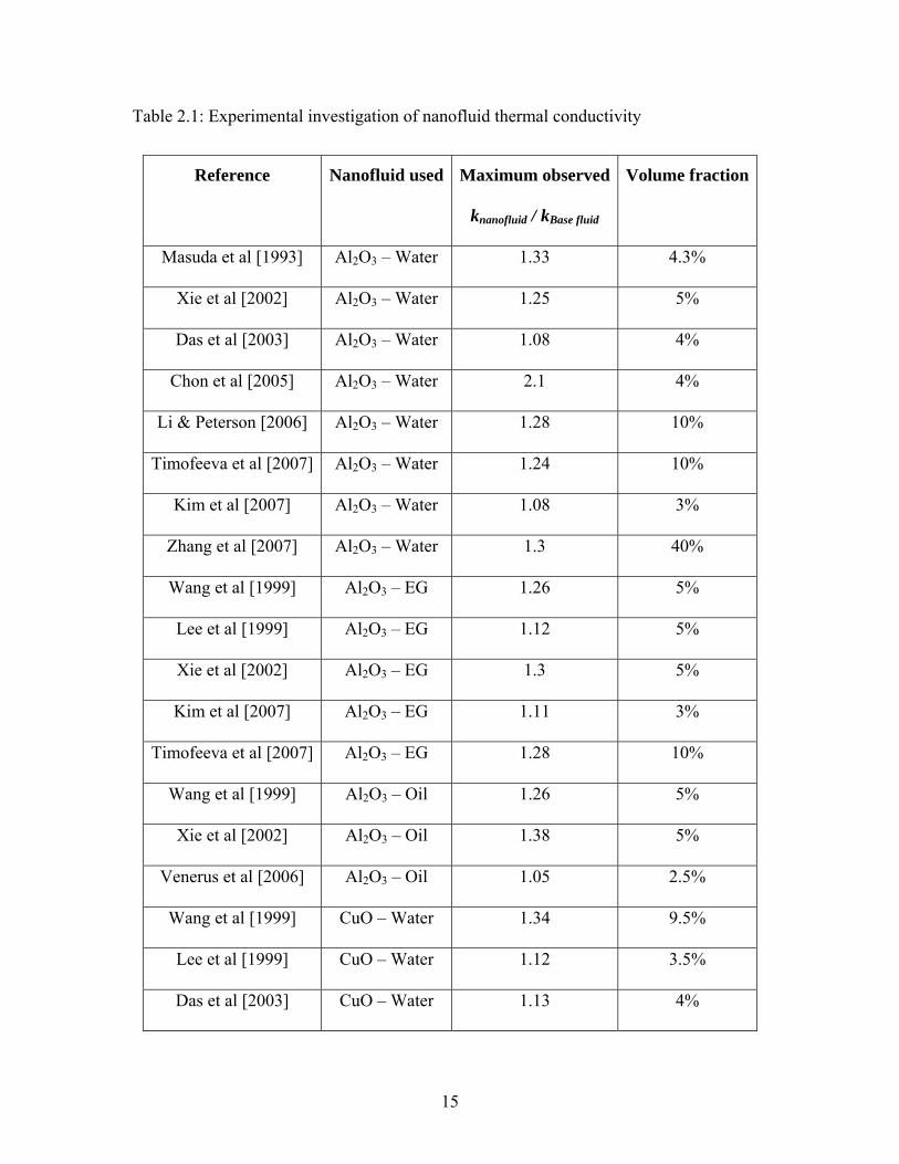
Table 2.1: Experimental investigation of nanofluid thermal conductivity
Reference Nanofluid used Maximum observed
knanofluid / kBase fluid
Volume fraction
Masuda et al [1993] Al2O3 – Water 1.33 4.3%
Xie et al [2002] Al2O3 – Water 1.25 5%
Das et al [2003] Al2O3 – Water 1.08 4%
Chon et al [2005] Al2O3 – Water 2.1 4%
Li & Peterson [2006] Al2O3 – Water 1.28 10%
Timofeeva et al [2007] Al2O3 – Water 1.24 10%
Kim et al [2007] Al2O3 – Water 1.08 3%
Zhang et al [2007] Al2O3 – Water 1.3 40%
Wang et al [1999] Al2O3 – EG 1.26 5%
Lee et al [1999] Al2O3 – EG 1.12 5%
Xie et al [2002] Al2O3 – EG 1.3 5%
Kim et al [2007] Al2O3 – EG 1.11 3%
Timofeeva et al [2007] Al2O3 – EG 1.28 10%
Wang et al [1999] Al2O3 – Oil 1.26 5%
Xie et al [2002] Al2O3 – Oil 1.38 5%
Venerus et al [2006] Al2O3 – Oil 1.05 2.5%
Wang et al [1999] CuO – Water 1.34 9.5%
Lee et al [1999] CuO – Water 1.12 3.5%
Das et al [2003] CuO – Water 1.13 4%
15
Reference Nanofluid used Maximum observed
knanofluid / kBase fluid
Volume fraction
Li & Peterson [2006] CuO – Water 1.52 6%
Wang et al [1999] CuO – EG 1.53 15%
Lee et al [1999] CuO – EG 1.21 4%
Hwang et al [2006] CuO – EG 1.05 1%
Kang et al [2006] SiO2 – Water 1.05 4%
Hwang et al [2006] SiO2 – Water 1.03 1%
Wang et al [2007] SiO2 – Water 1.03 1%
Wang et al [2007] SiO2 – EG 1.04 1%
Murshed et al [2005] TiO2 – Water 1.3 5%
Kim et al [2007] TiO2 – Water 1.11 3%
Zhang et al [2007] TiO2 – Water 1.07 3%
Murshed et al [2006] TiO2 – EG 1.18 5%
Kim et al [2007] TiO2 – EG 1.15 3%
Kang et al [2006] Ag – Water 1.11 0.4%
Patel et al [2003] Au – Water 1.05 0.01%
Kumar et al [2004] Au – Water 1.2 0.01%
Putnam et al [2006] Au – Ethanol 1.013 0.018%
Xuan & Li [2000] Cu – Water 1.24 2%
Liu et al [2006] Cu – Water 1.24 0.1%
Jana et al [2007] Cu – Water 1.7 0.3%
16
Reference Nanofluid used Maximum observed
knanofluid / kBase fluid
Volume fraction
Eastman et al [2001] Cu – EG 1.4 0.3%
Assael et al [2006] Cu – EG 1.03 0.48%
Eastman et al [1999] Cu – Oil 1.44 0.052%
Xuan & Li [2000] Cu – Oil 1.45 0.05%
Xie et al [2003] CNT – Water 1.07 1%
Assael et al [2006] CNT – Water 1.39 0.6%
Hwang et al [2007] CNT – Water 1.07 1%
Zhang et al [2007] CNT – Water 1.4 0.09%
Xie et al [2003] CNT – EG 1.12 1%
Choi et al [2001] CNT – Oil 2.6 1%
Hwang et al [2007] CNT – Oil 1.09 0.5%
17
It can be observed from Table 2.1 that nanofluids show significantly high thermal
conductivity compared to the base fluid even at small volume fraction of nanoparticles.
Some of the experimental data can be explained by models like Maxwell [1881] and
Hamilton-Crosser [1962], but the thermal conductivity data shows significant variation.
Different research groups have reported different enhancement in thermal conductivity
even for same nanofluid suspensions. Some of the noticeable results from Table 2.1 are
discussed here.
Masuda et al [1993] were the first group to do experiments with suspension of
nanometer size particles and report enhanced heat transfer. They used Al2O3, SiO2 and
other oxide nanoparticle in water and reported 30% increase in thermal conductivity of
base fluid suspended with Al2O3 nanoparticles at a volume fraction of 4.3%. They also
observed that the friction factor of the suspension increased 4 times at same volume
fraction. Choi [1995] was the first to use the term 'nanofluid' for the suspension of
nanometer size particles in heat transfer fluids. He conducted experiments at the Argonne
National Lab and reported a new class of engineered fluids consisting of nanometer sized
copper particles suspended in ethylene glycol. He reported almost 100% increase in the
thermal conductivity of base fluid at only 1% volume fraction of copper nanoparticles.
Eastman et al [1999] conducted experiments with Cu, Al2O3 and CuO
nanoparticles suspended in HE-200 oil and water. They reported a 40% enhancement in
conductivity of HE-200 oil at only 0.05% volume fraction of Cu nanoparticles. They
observed 29% increase in the thermal conductivity for Al2O3-water nanofluid at 5%
volume fraction and 60% increase in CuO-water nanofluid with 5% volume fraction of
18
35 nm CuO nanoparticles. They also reported a moderate 20% increase in the thermal
conductivity of ethylene glycol suspended with CuO nanoparticle at 4% volume fraction.
Lee et al [1999] did experimental study using Al2O3 and CuO nanoparticles
suspended in water and ethylene glycol and observed 15% enhancement in the thermal
conductivity of Al2O3-water nanofluid at the same volume fraction as Masuda et al
[1993]. The difference in their results was attributed to the size of nanoparticles used in
the two experiments. Masuda et al [1993] used 13 nm Al2O3 nanoparticles while Lee et al
[1999] used 33 nm nanoparticles. Wang et al [1999] measured the thermal conductivity
of nanofluids consisting of Al2O3 and CuO nanoparticles suspended in water and ethylene
glycol. They observed a maximum of 12% thermal conductivity enhancement for Al2O3
nanoparticles with a volume fraction of 3%.
Eastman et al [2001] reported a 40% thermal conductivity enhancement for Cu-
ethylene glycol nanofluid at 0.3% volume concentration of 10 nm Cu nanoparticles. This
high enhancement was observed when thioglycolic acid (1% volume concentration) was
added to the nanofluid suspension to aid dispersion of nanoparticles. Same nanofluid
suspension without the dispersant showed only 12% thermal conductivity enhancement.
They also conducted experiments with Al2O3 and CuO nanoparticles dispersed in
ethylene glycol and reported 18% enhancement for CuO-ethylene glycol nanofluid at 5%
volume fraction and 22% enhancement for Al2O3-ethylene glycol nanofluid at 4%
volume fraction.
Wang et al [2002] conducted experiments with several types of nanofluids. They
prepared nanofluids using ethylene glycol as base fluid dispersed with CuO, Al2O3 and
TiO2 nanoparticles. They measured the thermal conductivity of nanofluids using steady-
19
state parallel plate method. They reported 18% increase in thermal conductivity for
Al2O3-ethylene glycol nanofluid at 4% volume fraction. This is consistent with the
enhancement showed by Eastman et al [2001]. In contrast, Xie et al [2002] reported 30%
increase in thermal conductivity at 5% volume fraction for same nanofluid. However the
Al2O3 nanoparticles used by Wang et al were 29 nm in diameter and that used by Xie et
al were 60 nm in diameter. Xie et al [2002] also studied the effect of solution pH on the
thermal conductivity and observed that the thermal conductivity decreased with
increasing pH of the nanofluid. They concluded that among other parameters, the system
chemistry also plays a role in determining the thermal conductivity of nanofluids.
Patel et al [2003] used Au and Ag nanoparticles dispersed in water and toluene to
prepare nanofluid suspensions. They reported 4-7% increase in conductivity for Au-
toluene nanofluid at a vanishingly small 0.005-0.011% volume fraction of silver
nanoparticles. They also reported 3.2-5% increase in the conductivity of Ag-water
nanofluid at a very small conductivity of 0.0013-0.026% volume fraction of gold
nanoparticles. The same group later reported 20% increase in thermal conductivity of Au-
water nanofluid at a mere 0.00013% volume fraction [Kumar et al 2004]. They attributed
the anomalous increase in the thermal conductivity of nanofluids to very small size (4
nm) and very high thermal conductivity of the nanoparticles used. Putnam et al [2006]
used the same nanoparticle and base fluid combination (4 nm Au nanoparticles with
ethylene glycol) and reported only a moderate 1.3% ± 0.8% increase in the thermal
conductivity of nanofluid at 0.018% volume fraction. There results are in contrast to that
reported by Patel et al [2003] and Kumar et al [2004] for same nanofluid.
20
Murshed et al [2005], Murshed et al [2006] and Leong et al [2006] conducted
experiments with several types of nanofluids. They prepared nanofluids with water and
ethylene glycol as base fluid, suspended with Al, Al2O3 and TiO2 nanoparticles. They
reported 32% increase in thermal conductivity for TiO2–water nanofluid at 5% volume
fraction, 18% increase in thermal conductivity for TiO2–ethylene glycol nanofluid at
same volume fraction, and a much higher 49% enhancement in thermal conductivity for
Al–ethylene glycol nanofluid at the same volume fraction. They used cylindrical and
spherical TiO2 nanoparticles and observed higher enhancement for cylindrical
nanoparticles compared to spherical ones. They observed that nanofluids consisting of
higher conductivity nanoparticle (Al) showed higher thermal conductivity enhancement
compared to the nanofluids consisting of lower thermal conductivity nanoparticle (TiO2).
It is well known that carbon nanotubes (CNT) exhibit unusually high thermal
conductivities [Berber et al, 2000]. Carbon nanotubes (CNT’s) with their ultrafine size
and very high thermal conductivity attracted researchers to use CNT’s as the dispersed
solid phase in the nanofluids. Choi et al [2001] used multi-wall-carbon nanotubes
(MWCNT) in poly (α-olefin) oil and reported an astonishing 160% increase in thermal
conductivity of poly (α-olefin) oil at only 1% volume fraction of MWCNT having 25 nm
mean diameter and 50 µm length. They observed non-linear increase in thermal
conductivity at very small volume fractions (< 1%). They attributed this huge
enhancement in thermal conductivity of the nanofluid to the high thermal conductivity of
nanotubes and interaction between carbon fiber and fluid molecules. Xie et al [2003]
reported only 6% increase in thermal conductivity with MWCNT suspension in water at
1% volume fraction. Yang et al [2006] reported 200% increase in thermal conductivity of
21
poly (α-olefin) oil suspended with only 0.35% volume fraction of MWCNT. They also
reported a 3 times increase in the viscosity of poly (α-olefin) oil at same volume fraction
of MWCNT.
It was observed from experimental data that nanofluids consisting of
nanoparticles with very high thermal conductivity show anomalously high enhancement.
Hong et al [2005] conducted experiments with Fe–ethylene glycol based nanofluids and
reported 18% increase in thermal conductivity at only 0.55% volume fraction of iron
nanoparticles. They also observed that the sonication of the nanofluid suspension had a
significant effect on the thermal conductivity. Zhu et al [2006] also reported a high 38%
increase in thermal conductivity for Fe3O4–water based nanofluid at only 5% volume
fraction of. They attributed this high enhancement to the nanoparticles forming clusters.
These studies show that even nanofluids consisting of nanoparticles with relatively lower
thermal conductivity (Fe, Fe3O4) can produce high thermal conductivity enhancement.
From the above mentioned literature survey it is clear that the thermal
conductivity enhancement data shows a lot of scatter. Till date the data produced by one
group has not been reproduced by another group. It has been observed that many
parameters like nanoparticle-base fluid combination, particle volume fraction, size,
shape, system temperature and the choice of dispersant used to stabilize the suspension
affect the thermal conductivity of nanofluids. The effects of these parameters as reported
by various groups are also contradictory. A clear consensus has not been reached yet
among the scientific community on how each of these parameters affects the thermal
conductivity of nanofluids. Now some experimental studies showing the effect of particle
volume fraction, size and system temperature are discussed here.
22
2.1.1 Effect of Particle Volume Fraction
One point where the scientific community agrees about the thermal conductivity
enhancement in nanofluids is that the thermal conductivity increases almost linearly with
an increase in particle volume fraction. As shown in Figure 2.1, most of the experimental
data in the literature shows a linear thermal conductivity increase with volume fraction.
However, some exceptions have been reported to show non-linear increase in thermal
conductivity at low volume fractions (< 1%) [Choi et al 2001, Murshed et al 2005,
Hwang et al 2006]. Choi et al [2001] and Hwang et al [2006] used nanofluids consisting
of MWCNT in oil and observed quadratic relationship between thermal conductivity of
nanofluid with particle volume fraction at concentrations less than 1% as shown in Figure
2.2. Murshed et al [2005] in their experiments observed that the thermal conductivity
versus particle volume fraction curve can be divided into two linear regimes. The
transition typically occurred at volume fraction of around 1% as shown in Figure 2.3. Zhu
et al [2006] also observed the same behavior, but they observed the transition at around
2% volume fraction. While some researchers have reported anomalous thermal
conductivity enhancements at particle volume fractions less than 1% for metallic
nanoparticles [Eastman et al 2001, Patel et al 2003, Kumar et al 2004, Jana et al 2007],
other have reported conductivity enhancement that can be explained by classical models
[Wang et al 2002, Xie et al 2002, Putnam et al 2006, Zhu et al 2006].
23
φ (%)
0 1 2 3 4 5 6
(kef
f - k
f) / k
f (%
)
0
5
10
15
20
25
Eastman et al [1999], Al2O3 in H2OEastman et al [1999], CuO in H2O
Figure 2.1: Thermal conductivity of aqueous nanofluids as measured by Eastman et al
[1999]. The straight lines represent linear fit to the data.
24
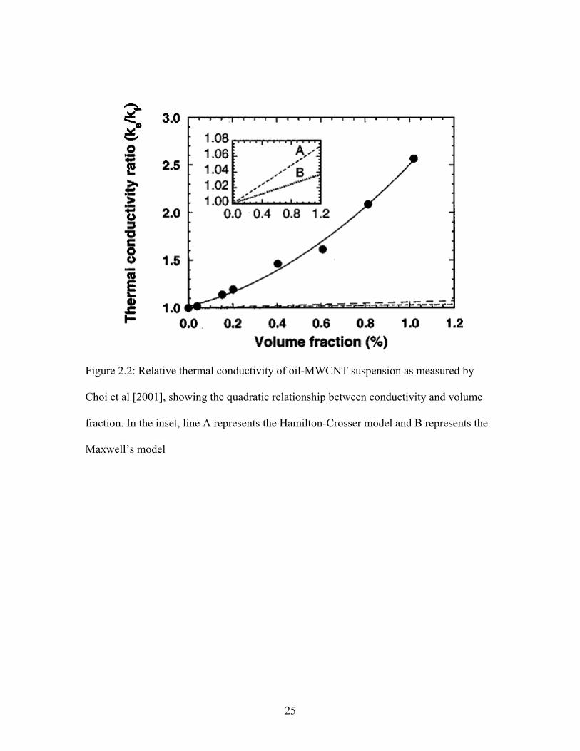
Figure 2.2: Relative thermal conductivity of oil-MWCNT suspension as measured by
Choi et al [2001], showing the quadratic relationship between conductivity and volume
fraction. In the inset, line A represents the Hamilton-Crosser model and B represents the
Maxwell’s model
25
φ (%)
0 1 2 3 4 5 6
(kef
f - k
f) / k
f (%
)
0
5
10
15
20
25
30
35
Murshed et al [2005], SphereMurshed et al [2005], Cylinder
Figure 2.3: Thermal conductivity enhancement of nanofluids consisting of TiO2 in water
as measured by Murshed et al [2005], showing the two regimes of conductivity
enhancement with volume fraction. The lines represent linear fit to the data.
26
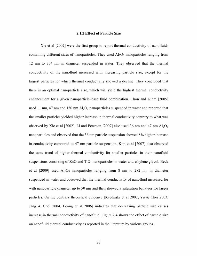
2.1.2 Effect of Particle Size
Xie et al [2002] were the first group to report thermal conductivity of nanofluids
containing different sizes of nanoparticles. They used Al2O3 nanoparticles ranging from
12 nm to 304 nm in diameter suspended in water. They observed that the thermal
conductivity of the nanofluid increased with increasing particle size, except for the
largest particles for which thermal conductivity showed a decline. They concluded that
there is an optimal nanoparticle size, which will yield the highest thermal conductivity
enhancement for a given nanoparticle–base fluid combination. Chon and Kihm [2005]
used 11 nm, 47 nm and 150 nm Al2O3 nanoparticles suspended in water and reported that
the smaller particles yielded higher increase in thermal conductivity contrary to what was
observed by Xie et al [2002]. Li and Peterson [2007] also used 36 nm and 47 nm Al2O3
nanoparticles and observed that the 36 nm particle suspension showed 8% higher increase
in conductivity compared to 47 nm particle suspension. Kim et al [2007] also observed
the same trend of higher thermal conductivity for smaller particles in their nanofluid
suspensions consisting of ZnO and TiO2 nanoparticles in water and ethylene glycol. Beck
et al [2009] used Al2O3 nanoparticles ranging from 8 nm to 282 nm in diameter
suspended in water and observed that the thermal conductivity of nanofluid increased for
with nanoparticle diameter up to 50 nm and then showed a saturation behavior for larger
particles. On the contrary theoretical evidence [Keblinski et al 2002, Yu & Choi 2003,
Jang & Choi 2004, Leong et al 2006] indicates that decreasing particle size causes
increase in thermal conductivity of nanofluid. Figure 2.4 shows the effect of particle size
on nanofluid thermal conductivity as reported in the literature by various groups.
27
Particle Diameter (nm)
0 10 20 30 40 50 60 70 80
(Kef
f - K
f) / K
f (%
)
0
5
10
15
20
25
30
35
Xie et al [2003]Li & Peterson [2007]Chon & Kihm [2003]Kim et al [2007]Beck et al [2008]
Figure 2.4: Thermal conductivity enhancement of nanofluids as a function of particle
size, as measured by various groups
28
2.1.3 Effect of System Temperature
Nanofluids have been proposed to be used in a wide variety of engineering
applications due to their promising thermal transport properties. Some of these
applications may involve high temperatures, which could play an important role in the
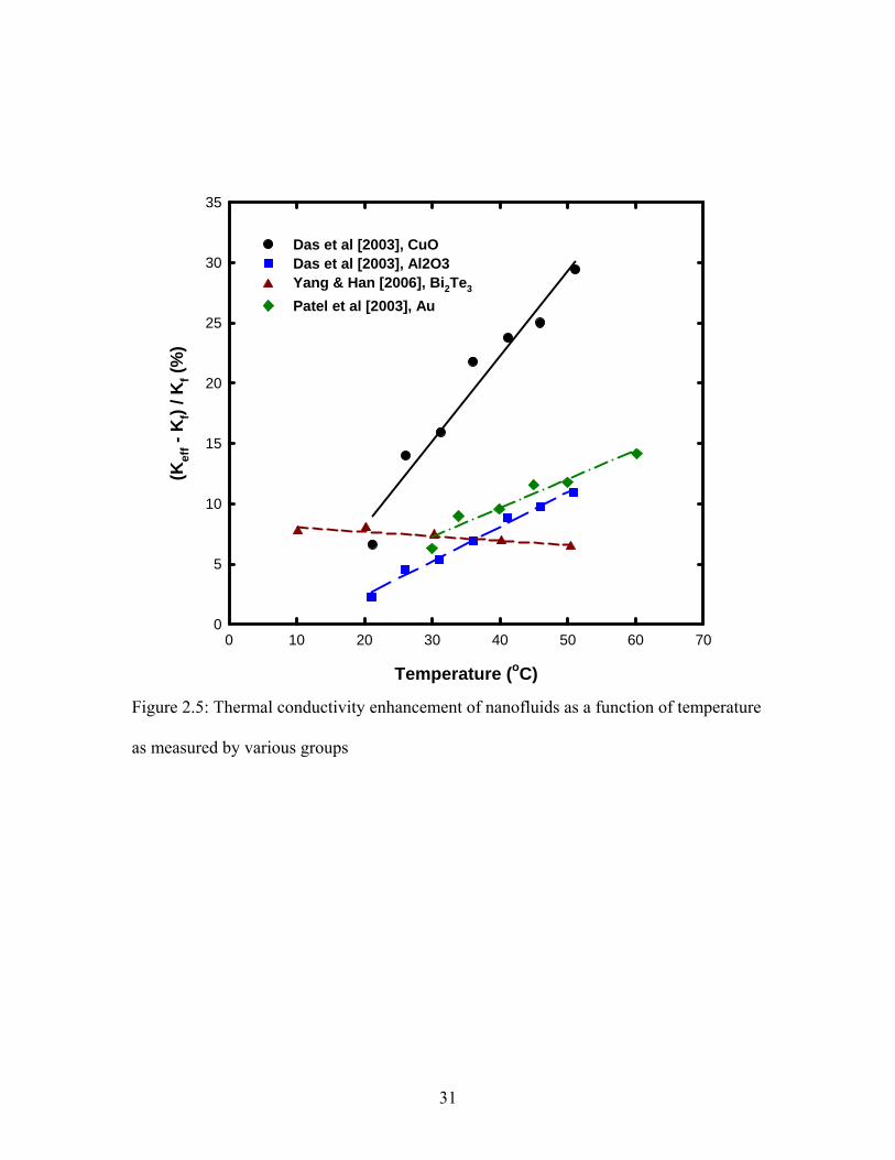
thermal conductivity enhancement of nanofluids. Das et al [2003] experimentally studied
nanofluids consisting of Al2O3 and CuO nanoparticles suspended in water at elevated
temperatures. They reported that the thermal conductivity of Al2O3–water nanofluid
increased from 16-25% and for CuO–water nanofluid increased from 22-30% as the
suspension temperature was increased from 21-51˚C. The same group later used Au–
water nanofluid [Patel et al 2003] and reported thermal conductivity increase from 5-21%
at 0.026% volume fraction as the temperature was increased from 30-60˚C. They
suggested that this strong temperature dependence on thermal conductivity of nanofluids
was due to the Brownian motion of nanoparticles. They also speculated that this
temperature dependence will remain the same even at higher fluid temperatures. Chon
and Kihm [2005] also used Al2O3–water nanofluid and reported a moderate increase of 6-
11% in thermal conductivity as the nanofluid temperature was raised from 31-51˚C.
Murshed et al [2006] also reported a moderate increase in thermal conductivity by 9% for
Al2O3–water nanofluid as the system temperature was increased from 30-60˚C. Li &
Peterson [2007] also used Al2O3–water nanofluid and reported thermal conductivity
enhancement from 7-23% at 2% volume fraction as the system temperature was increased
from 27-36˚C.
29
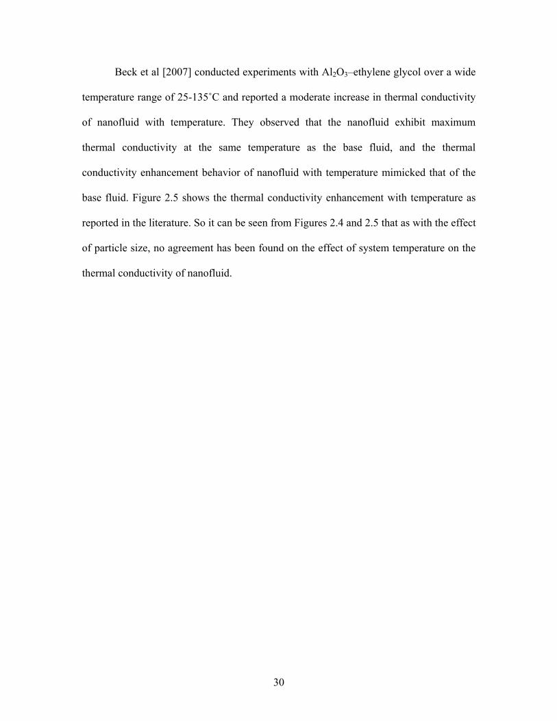
Beck et al [2007] conducted experiments with Al2O3–ethylene glycol over a wide
temperature range of 25-135˚C and reported a moderate increase in thermal conductivity
of nanofluid with temperature. They observed that the nanofluid exhibit maximum
thermal conductivity at the same temperature as the base fluid, and the thermal
conductivity enhancement behavior of nanofluid with temperature mimicked that of the
base fluid. Figure 2.5 shows the thermal conductivity enhancement with temperature as
reported in the literature. So it can be seen from Figures 2.4 and 2.5 that as with the effect
of particle size, no agreement has been found on the effect of system temperature on the
thermal conductivity of nanofluid.
30
Temperature (oC)
0 10 20 30 40 50 60 70
(Kef
f - K
f) / K
f (%
)
0
5
10
15
20
25
30
35
Das et al [2003], CuODas et al [2003], Al2O3Yang & Han [2006], Bi2Te3
Patel et al [2003], Au
Figure 2.5: Thermal conductivity enhancement of nanofluids as a function of temperature
as measured by various groups
31
2.2 Modeling of Nanofluids
It is evident that a significant experimental research has been conducted in
determining the heat transport characteristics of the nanofluids in last decade, but still
many questions remain unanswered. The data produced by one group is not reproducible
by another and no concrete theory has been established to predict the thermal
conductivity of nanofluids and explain the anomalous enhancement. Researchers have
proposed many theories to explain the anomalous behavior observed in nanofluids. The
early attempts to explain the enhanced transport characteristics of nanofluids were made
with the classical theory of Maxwell [1881] for composite materials. This theory was
developed to calculate the electrical or thermal conductivity of dilute solid–liquid
suspension of spherical particles at low volume fractions. It is applicable to homogeneous
isotropic solution of uniformly sized solid particles randomly dispersed in a fluid.
2 2 (2 (
p f p fe
f p f p f
k k k kkk k k k k
))
φφ
+ + −=
+ − − (2.1)
Here ke is the effective thermal conductivity of the suspension, kf is the thermal
conductivity of the base fluid, kp is the thermal conductivity of nanoparticle, φ is the
volume fraction. This theory is also appropriate for predicting properties such as
dielectric constant and magnetic permeability of composite materials. When compared
with experimental data Maxwell’s theory matched well for low particle concentrations
with spherical particles of millimeter or micrometer size, but it did not conform well to
particles of nanometer size and non-spherical shapes.
32

Hamilton and Crosser [1962] (HC) extended Maxwell’s model and generalized it
for non-spherical particles. They came up with an expression for effective thermal
conductivity of a colloidal suspension as:
( ) ( )( )1 1 (
1 ( )p f pe
f p f p f
k n k n k kkk k n k k k
φφ
+ − + − −=
+ − − −
)f (2.2)
Here, n is the non-spherical shape factor given as:
3 nψ
= (2.3)
Here, ψ is the sphericity, defined as the ratio of the surface area of a sphere with
volume equal to that of the particle to the surface area of the particle. For n=3 HC model
reduces to Maxwell model for spherical particles. The HC theory was used by Xuan & Li
[2000] to obtain rough estimation of thermal conductivity of nanofluids for different
volume fraction and shape factor. They showed that for ψ=0.7 the HC model predicts
results close to their experimental results. Lee et al [1999] showed that HC model
predicted the right trend for oxide particles, but when used for very fine metallic particles
[Eastman et al, 2001] it under-predicted the effective thermal conductivity by over an
order of magnitude. Classical models like Maxwell and HC model can not explain or
predict the nanofluid thermal conductivity data because they do not include the effect of
particle size, shape, interfacial layer at the solid-liquid interface, system temperature and
the Brownian motion of the particles, which have been found to affect the thermal
conductivity of nanofluids. It was not surprising that both Maxwell’s model and HC
model were not able to predict the enhancement in thermal conductivity of nanofluids
because they did not take into account various important parameters affecting the heat
transport in nanofluids and modes of thermal transport in nanostructures.
33
Many theoretical studies have been conducted in recent past to explain and predict
the anomalous thermal conductivity increase in nanofluids. Several theoretical models
have been proposed which include the effect of various parameters like the particle size,
system temperature and liquid layer at the solid-liquid interface. Keblinski et al [2002]
attribute the enhancement in thermal conductivity to four possible mechanisms,
Brownian motion of particles, layering of liquid molecules around the particles, ballistic
nature of heat transport in nano-structures and nanoparticle clustering. Particles move
through liquid by Brownian motion and collide with each other, hence enabling direct
solid-solid transport of heat from one to another.
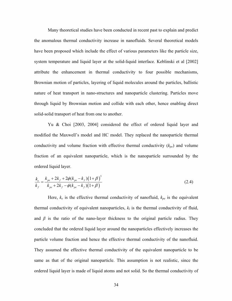
Yu & Choi [2003, 2004] considered the effect of ordered liquid layer and
modified the Maxwell’s model and HC model. They replaced the nanoparticle thermal
conductivity and volume fraction with effective thermal conductivity (kpe) and volume
fraction of an equivalent nanoparticle, which is the nanoparticle surrounded by the
ordered liquid layer.
( )( )
32 2 ( ) 12 ( ) 1
pe f pe fe
f pe f pe f
k k k kkk k k k k
φ βφ β
+ + − +=
+ − − + (2.4)
Here, ke is the effective thermal conductivity of nanofluid, kpe is the equivalent
thermal conductivity of equivalent nanoparticles, kl is the thermal conductivity of fluid,
and β is the ratio of the nano-layer thickness to the original particle radius. They
concluded that the ordered liquid layer around the nanoparticles effectively increases the
particle volume fraction and hence the effective thermal conductivity of the nanofluid.
They assumed the effective thermal conductivity of the equivalent nanoparticle to be
same as that of the original nanoparticle. This assumption is not realistic, since the
ordered liquid layer is made of liquid atoms and not solid. So the thermal conductivity of
34
this ordered liquid layer at the solid-liquid interface would be in between the thermal
conductivity of the liquid and the solid. Another unknown in their model was the
thickness of this ordered liquid layer.
Xue et al [2003] proposed a model based on Maxwell’s theory and average
polarization theory, which also includes the effect of the ordered liquid layer. To validate
their model with experimental data from Choi et al [2001], they used 2 incorrect
parameters. Later when they used the corrected parameters Yu & Choi [2003] showed
that this model predicted thermal conductivity of the nanofluid to be 32 times that of the
base fluid. So this model has not been validated and its accuracy is yet to be established.
Wang et al [2003] modified Maxwell’s model to include the effect of nanoparticle
clustering and polarization. To predict the thermal conductivity of the nanofluid their
model requires effective thermal conductivity and radius distribution of the nanoparticle
cluster, which have to be determined numerically. This model is also yet to be validated
with experimental data.
Other models have also been proposed by Jang & Choi [2004], Kumar et al
[2004], Prasher et al [2005], Ren et al [2005], and Leong et al [2006]. Each of these
models is based on one or more of the following thermal conduction mechanism in
nanofluids (a) collision between base fluid molecules, (b) thermal diffusion in
nanoparticles in fluid, (c) collision between nanoparticles due to Brownian motion, (d)
thermal interaction between nanoparticle and base fluid molecules, (e) ordered liquid
layer at the solid-liquid interface, or (f) nanoparticle clustering. These mechanisms have
been proposed to be the origin of enhanced thermal properties of nanofluids. Since all
these mechanisms involve interaction occurring at nano-scale, there is no direct way to
35
verify the presence of any of these mechanisms by macro-scale experiments like
Transient Hot Wire, Oscillating Parallel Plate, or Optical Beam Deflection methods
which have been used to measure the thermal conductivity in nanofluids. Some modeling
method that can simulate the interaction between the solid nanoparticles and fluid
molecules at nano-scale is required to validate the presence of these mechanisms.
2.3 Computer Simulations of Nanofluids
Several attempts have been made to study the nanofluids using simulation
methods that can capture the complex thermal transport phenomenon occurring in
nanofluids at the nanoscale. Molecular dynamics simulation, an atomic-scale simulation
technique that can track the motion of solid and liquid atoms at molecular level has been
used in these simulation studies. A list of molecular simulation studies performed on
nanofluids is presented in Table 2.2 and some of the notable simulation studies on
nanofluids are discussed here.
36
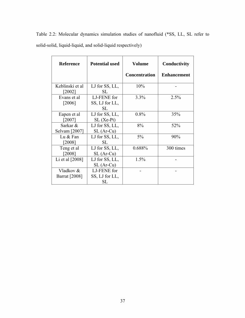
Table 2.2: Molecular dynamics simulation studies of nanofluid (*SS, LL, SL refer to
solid-solid, liquid-liquid, and solid-liquid respectively)
Reference Potential used Volume
Concentration
Conductivity
Enhancement
Keblinski et al [2002]
LJ for SS, LL, SL
10% -
Evans et al [2006]
LJ-FENE for SS, LJ for LL,
SL
3.3% 2.5%
Eapen et al [2007]
LJ for SS, LL, SL (Xe-Pt)
0.8% 35%
Sarkar & Selvam [2007]
LJ for SS, LL, SL (Ar-Cu)
8% 52%
Lu & Fan [2008]
LJ for SS, LL, SL
5% 90%
Teng et al [2008]
LJ for SS, LL, SL (Ar-Cu)
0.688% 300 times
Li et al [2008] LJ for SS, LL, SL (Ar-Cu)
1.5% -
Vladkov & Barrat [2008]
LJ-FENE for SS, LJ for LL,
SL
- -
37

Keblinski et al [2002] used equilibrium molecular dynamics simulation to
qualitatively study a model nanofluid system. Their simulation domain consisted of a
single 2 nm diameter solid nanoparticle surrounded by fluid molecules in a cubic box of
length 3.5 nm with 10% particle volume fraction. Lennard-Jones potential was used to
simulate the interactions between all atoms pairs, solid-solid, liquid-liquid and solid-
liquid. The Lennard-Jones energy parameter (εss) for solid atoms was 10 times that used
for the liquid atoms (εll). By comparing the heat current autocorrelation function (HCAF)
between solid and liquid atoms, they observed that the HCAF for liquid atoms decayed
monotonically, while that for solid atoms decayed in an oscillatory manner. By this
comparison they concluded that heat moves in a ballistic manner inside the solid
nanoparticle and the particle-liquid interface plays a key role in translating fast thermal
transport in solid particles into high overall thermal conductivity of the nanofluid. No
quantitative information on the extent of heat transfer enhancement was provided in this
study.
Wu and Kumar [2004] used non-equilibrium molecular dynamics (NEMD)
simulation to calculate the thermal conductivity of nanofluid. A brief description of the
NEMD method is given in the next section. They considered all the interactions, fluid-
fluid, particle-particle and fluid-particle possible in a nanofluid suspension. They used a
Lennard-Jones like potential to simulate the fluid-fluid and particle-fluid interactions and
another inter-atomic potential was used for particle-particle interactions. The particle-
particle potential takes into account the size of the particles also. They used perfectly
elastic collisions between particles to simulate the non-agglomerated case and perfectly
inelastic collision method to simulate to agglomeration between nanoparticles. The
38
results for non-agglomerated system match fairly well with the experimental results for
nanofluid consisting of 10 nm copper nanoparticles with water. The random Brownian
motion of particles show a strong dependence on temperature and the frequency of
collision between fluid molecules and nanoparticle increases with temperature, therefore
the effective thermal conductivity of the suspension also increases. It was also observed
that the agglomeration between nanoparticles decreases the heat transfer enhancement,
particularly at low concentration, since the agglomerated particles tend to settle down in
liquid and also reduce the number density of particles, which creates large regions of
particle-free liquid. It was also shown that the effective thermal conductivity of nanofluid
decreases as the number of agglomerated nanoparticles increases. Although this work
used simple potential functions to simulate the interactions, but it gives good insight into
the difference between agglomerated and non-agglomerated system and the results also
match well with experiments.
Bhattacharya et al [2004] carried out Brownian dynamics simulation with
equilibrium Green-Kubo method to calculate effective thermal conductivity of nanofluid
and found good agreement with experimental results, but their results depend on the
correlated parameters, which were used to match with their experimental data and are
difficult to apply in other nanofluid data as there is no systematic way to find these
parameters. Although initial calculations showed significant increases in thermal
conductivity from Brownian motion of particles, interaction parameters based on
appropriate Debye length increased the conductivity by less than 2% [Gupta et al, 2007].
Eapen et al [2007] did an order of magnitude analysis between thermal diffusion and
Brownian diffusion and showed that even for extremely small particles thermal diffusion
39
is much faster than Brownian diffusion, so they concluded that Brownian effects are
small in heat transport in nanofluids.
Evans et al [2006] performed NEMD simulation of a single solid nanoparticle
surrounded by liquid atoms. The interactions between the atoms in the solid nanoparticle
and between fluid atoms were simulated using Lennard-Jones potential. The atoms in the
solid nanoparticle were connected with their nearest neighbor using finite extension non-
linear elastic (FENE) bonding potential. They observed a modest 2.5% increase in the
thermal conductivity of nanofluid at 3.3% particle volume fraction. This enhancement is
lower compared to that observed in any experimental study but is close to that predicted
by effective medium (EM) theory [Putnam et al 2003] for well-dispersed thermal
conductive nanoparticles.
Eapen et al [2007] conducted equilibrium molecular dynamics (EMD) simulation
of a model nanofluid using Lennard-Jones potential to simulate the solid-solid, liquid-
liquid and solid-liquid interaction. They used sub-nanometer size nanoparticles consisting
of 10 atoms surrounded by liquid atoms in a cubic simulation domain. They used a
repulsive potential between the nanoparticles to stop them from agglomerating. The
number of nanoparticles was varied to study the effect of particle volume fraction on
thermal conductivity. They used the Lennard-Jones energy (ε) and length parameter (σ)
of Xe for liquid atoms and Pt for solid atoms. The parameters for solid-liquid interactions
were calculated using the classical Lorentz-Berthelot mixing rule [Allen & Tildesley,
1987]. Green-Kubo correlation was used to calculate the thermal conductivity of the
nanofluid. They observed a maximum of 35% increase in thermal conductivity at 0.8%
particle volume fraction. They decomposed the heat current in to 3 constituents, namely
40
(a) Kinetic, (b) Potential, and (c) Collision modes and found that highest contribution to
the thermal conductivity came from the collision mode, which represents the interactions
between various atoms, but the enhancement in conductivity came mainly from the
potential energy mode. They concluded that the enhancements arise from the strong
solid-fluid attraction through the self correlation of the potential flux and that
enhancement was primarily a surface phenomenon. The interfacial fluid atoms form a
dynamic layer around the nanoparticle where potential energy is cooperatively exchanged
between solid and fluid atoms causing the enhanced thermal transport in nanofluids.
Sarkar & Selvam [2007] also used Lennard-Jones potential to model solid and
liquid atoms in their study of nanofluid system using molecular dynamic simulation.
They used the Lennard-Jones energy (ε) and length parameter (σ) of Ar [Allen &
Tildesley, 1987] for liquid atoms and Cu [Yu & Amar, 2002] for solid atoms. The
parameters for solid-liquid interactions were calculated using the classical Lorentz-
Berthelot mixing rule. Green-Kubo correlation was used to calculate the thermal
conductivity of the nanofluid. They observed an increasing thermal conductivity with
increasing particle volume fraction and reported a maximum enhancement of 52% at 8%
particle volume fraction. They observed two regimes of conductivity enhancement as
observed in the experiments by Murshed et al [2006]. The conductivity rose faster at
small volume fractions and showed a saturation behavior at larger volume concentration.
They studied the effect of particle volume fraction on thermal conductivity by varying the
size of solid particle and keeping the number of liquid atoms constant at 2048. As it has
been observed in the experiments that the particle volume fraction and size both affect the
thermal conductivity of nanofluid, this approach of varying particle size to study the
41
effect of volume fraction will not be able to distinguish between the parameters causing
the actual thermal enhancement. They compared the mean square displacement (MSD) of
liquid atoms in the nanofluid to that with the liquid atoms in the base fluid and found that
MSD was higher for nanofluid with higher volume concentration of solid. They
concluded that the thermal enhancement in nanofluids is caused by the enhanced motion
of the liquid atoms due to the presence of the solid nanoparticles.
Teng et al [2008] also used the same approach as used by Sarkar & Selvam
[2007] with same Lennard-Jones parameters for solid and liquid molecules. They studied
the effect of particle size at constant volume fraction and reported an increase in thermal
conductivity with increasing particle size. They reported an astonishing 300 times
increase in the thermal conductivity of nanofluid at a volume concentration of 0.688%. In
their words “This tremendous increase in thermal conductivity is amazing and needs to
be verified, or modified with discussion.” So their quantitative results on thermal
conductivity need to be verified. They decomposed the heat current used in Green-Kubo
correlation in convective and interatomic terms, and observed that the contribution of the
convective mode is higher compared to diffusion mode or the interatomic mode. This
finding is in contrast to previous findings by Eapen et al [2007] and Sarkar & Selvam
[2007].
Li et al [2008] also used a model nanofluid system with Lennard-Jones potential
to simulate interactions between all atom pairs. They also used Lennard-Jones parameters
of Ar for liquid and Cu for solid atoms. They did not report any quantitative results for
thermal conductivity but showed the presence of a layer of liquid molecules at the solid-
liquid interface. They compared the number density of liquid atoms in concentric shells
42

outside the solid nanoparticle to that with the number density of liquid atoms in base
fluid. They observed that the thickness of this ordered liquid layer was about 0.5 nm and
concluded that this ordered liquid layer is an important phenomenon causing the thermal
enhancement in nanofluids.
Although significant work has gone in experimentally measuring the thermal
conductivity of nanofluids, not much work has been performed in studying various
mechanisms of heat transport in nanofluids using computer simulations. As seen by the
few simplistic studies done on nanofluids using molecular dynamic simulation, it is clear
that this method shows promise in finding and confirming various nanoscale heat
transport mechanisms occurring in nanofluids. All the molecular dynamic studies
conducted till date have used the simplistic Lennard-Jones potential to model the solid-
solid, solid-liquid and liquid-liquid interactions. As discussed later in chapter 3 the choice
of interaction potential used in a molecular dynamic simulation determines the accuracy
and closeness to real experiment. There is a need to systematically study the various
mechanisms postulated by researchers using more realistic interaction potentials to
understand the phenomenon occurring at nano-scale in the nanofluids. A small literature
review of the molecular dynamic simulation technique and two ways of calculating
thermal conductivity using the same are discussed in the next section.
2.4 Literature Review on Molecular Dynamics Simulation
Molecular dynamics is a very powerful computer simulation technique where the
time evolution of a set of interacting atoms is studied by numerically integrating their
equations of motion. Molecular dynamics essentially involves solving a classical many-
43
body problem in the context of the study of matter at the atomic scale. It allows
predicting the static and dynamic properties of the system under consideration. For
complex systems which are modeled poorly by continuum or analytical methods,
Molecular dynamics simulation lends itself as a very good computational tool. Molecular
dynamics has been used to support research in the areas of physics, chemistry, biology
and materials science. Alder & Wainwright [1959] were amongst the first ones to do
molecular dynamics simulation in 1959 at the Lawrence Livermore National Laboratory.
They used a “hard sphere” model to study the molecules in liquid which interact as
“billiard balls”. They were able to simulate 32 and 108 molecules in computations
requiring 10 to 30 hours with the fastest computers at that time, an IBM 704. Rahman
[1964] studied many properties of liquid argon using Lennard-Jones potential on a system
containing 864 atoms. Verlet [1967] calculated the phase diagram of argon using
Lennard-Jones potential and computed correlation functions to test theories of liquid
state. Most of the systems studied at that time contained a very small number of atoms
but now with improvements in computer architecture it is possible to simulate millions of
particles but the computations continue to be demanding.
2.4.1 Thermal Conductivity Calculation using Molecular Dynamics Simulation
Experimentally, thermal conductivity (λ) is typically calculated by measuring the
temperature gradient that results from the application of a heat current. The thermal
conductivity relates the heat current to the temperature gradient via Fourier’s law as:
∑ ∂∂
−=ν ν
μνμ λxTJ (2.5)
44
Here Jμ is a component of the thermal current, λμv is an element of the thermal
conductivity tensor, and is the gradient of the temperature. In molecular
dynamics simulations the thermal conductivity can be computed either using the non-
equilibrium molecular dynamic (NEMD) [Müller-Plathe, 1997] or equilibrium molecular
dynamic (EMD) simulations [Vogelsang et al, 1987]. The two most commonly applied
methods in molecular dynamics are the ‘direct method’ and the Green-Kubo method. The
direct method is an NEMD method in which a temperature gradient is applied across the
simulation cell, essentially mimicking the experimental situation. On the other hand, in
the EMD method we use the Green-Kubo correlation, which uses the heat current
fluctuations to compute the thermal conductivity via the fluctuation-dissipation theorem
in the linear response of the system.
νxT ∂∂ /
As mentioned above the NEMD or direct method of computing the thermal
conductivity is analogous to the experimental measurement. Wu and Kumar [2004] used
NEMD method to calculate the thermal conductivity of suspension of copper
nanoparticles in water. Figure 2.6 shows a schematic representation of the simulation
domain used in this study to compute the thermal conductivity by Wu and Kumar [2004].
45
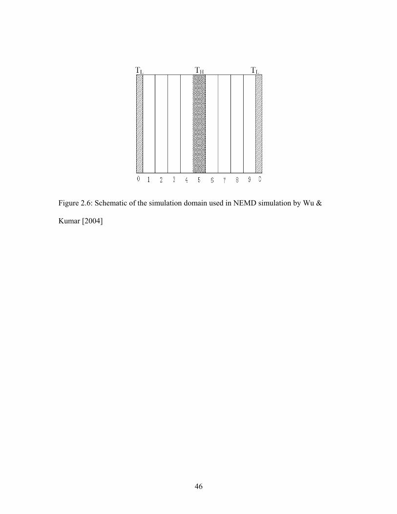
Figure 2.6: Schematic of the simulation domain used in NEMD simulation by Wu &
Kumar [2004]
46
The simulation domain was divided into 10 layers with each layer having
identical thickness and volume. Layer 0 was further divided into 2 equidistant parts to be
consistent with the periodic boundary condition. Layer 0 is defined as the “cold” layer
and layer 5 as the “hot” layer (Figure 2.6). The initial temperature of whole system is
maintained somewhere in between TH and TL.
By exchanging the particles (fluid molecules and nanoparticles) with highest
velocity in the cold layer with the ones having lowest velocity in the hot layer, the heat
flux is generated in the system. By exchanging the velocities, the temperature in the hot
layer increases and in the cold layer decreases, setting a temperature gradient in the
system. This temperature gradient leads to an energy transfer from the hot layer to the
cold layer by heat conduction. Total momentum, kinetic energy and total energy are kept
constant in this exchange process.
When the system reaches steady state, the heat flow due to velocity exchange of
particles must equal the heat conduction from the hot layer to the cold layer in both
directions. The energy balance can be written as:
∑ ∑= ∂
∂−=−
1,0
2,
2, 2)(
2i transferyzcihi
i
xTtAvvm λ (2.6)
Here, mi is the mass of the particle (i=0, 1 refer to the fluid molecule and
nanoparticle respectively), vh and vc are the velocity of particles in hot and cold layers
respectively, Ayz is the cross section area of calculated domain and t is the thickness of the
layer. All the quantities in equation (2.4) are exactly known, except the temperature
gradient. The temperature gradient has to be calculated using the kinetic theory of gases,
which relates temperature with velocity of particles as follows:
47
∑∑=
=i
n
jiji
Bik vm
knT
1
2,3
1 (2.7)
Here Tk is the instantaneous local temperature of layer k, ni is the number of ith
particle in layer k, vj,i is the velocity of ith particle in layer k, and kB is the Boltzmann
constant. Using the atomic velocities calculated at each molecular dynamic time step we
can calculate the temperature of hot and cold layer from equation (2.7) and then calculate
the temperature gradient. The left hand side of equation (2.6) is already known and by
plugging in the temperature gradient we can calculate the thermal conductivity of the
simulation domain.
As we observe in Figure 2.6, the application of hot and cold layer (source and
sink) and application of periodic boundary condition only generates a heat current in the
x-direction and with a single simulation thermal conductivity only along one particular
direction can be calculated. To obtain λ along a different crystal lattice direction, an
entirely new simulation domain with layers along the required lattice direction must be
created and new simulation must be carried out. This limitation does not exist for the
Green-Kubo method, where the entire thermal conductivity tensor is computed in just one
simulation. For the direct method, it is important that a steady-state heat current flow has
been achieved. This can be achieved by plotting a stationary temperature profile as a
function of time, thus insuring that only steady-state currents are flowing and, hence
thermal conductivity can be computed using equation (2.6).
In EMD simulation, Green-Kubo correlation of the heat current is used to
compute the thermal conductivity. In EMD simulation there is no imposed driving force
on the system, and hence the system is always in the linear-response regime. Since the
simulation is done in equilibrium and the system response in the linear regime, according
48
to the fluctuation-dissipation theorem, the transport coefficients can be calculated using
the Green-Kubo correlations [McQuarrie, 2000]. As mentioned earlier one major
advantage of Green-Kubo method over the NEMD method is that complete anisotropic
thermal conductivity of the system can be calculated in one simulation. While in the case
of direct method or NEMD, 3 separate simulations need to be run to calculate
conductivity in 3 directions. So in this work the EMD simulation with Green-Kubo
correlation is used to calculate the thermal conductivity of nanofluids. Details of the
linear response theory as used with EMD simulation are given in the next chapter.
49
CHAPTER THREE: METHODOLOGY
The basic assumption of continuum that the properties of material e.g.
temperature does not change very fast with change in time and space breaks down at the
nano-scale. At the nano-scale, properties of materials change at the atomic scale and so
the continuum methods like computational fluid dynamics (CFD) and finite element
methods (FEM) can not be used to simulate these systems. No conventional equations or
correlations are available to analyze the systems at the micro and nano-scale.
Experiments can be performed to measure macro-scale properties of these systems, but
experiments may have to be repeated several times which would increase the cost. So the
only feasible method to systematically study these phenomena occurring at molecular
level is by way of numerical experiments.
Figure 3.1 [Smith G., 1999] shows different numerical methods that can be used
at various length and time scales. At millimeter length scale the assumptions used to
derive continuum level equations are valid so we can use Navier-Stokes equations for
fluid flow at this scale. Conventional finite element modeling or computational fluid
dynamics numerical methods can be used to simulate the fluid flow and heat transfer at
this scale. When the dimensions are of the order of a few hundred micro-meters, these
conventional methods may still be used with reasonable accuracy. As we move to sub-
micrometer dimensions the assumptions used in the continuum models do not hold and
we can not use these conventional methods to appropriately model the systems with sub-
micrometer length scales. At this scale, Monte Carlo (MC) method or Lattice Boltzmann
50
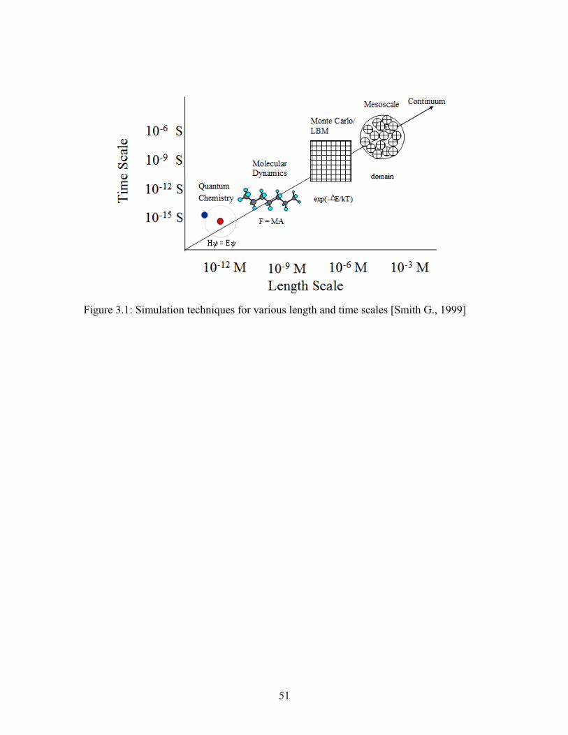
Figure 3.1: Simulation techniques for various length and time scales [Smith G., 1999]
51
Method (LBM) numerical techniques can be used to accurately simulate the fluid flow
and heat transfer.
As we move to nano-scale length scales MC and LBM also can not be used to
simulate the atomic scale system. At this scale, we should use a numerical technique
which deals with individual atoms and molecules. Molecular dynamics simulation is an
appropriate method to simulate the systems involving atomic size length scales. As the
length scale decreases further and we deal with individual electrons quantum chemistry
based methods e.g. quantum Molecular dynamics or density functional theory methods
should be used to model the systems.
To analyze flows in nanochannels, conventional finite element modeling or
computational fluid dynamics approach can not be used as these models break down at
micro-scale when the mean free path and the system size become of same order.
Molecular dynamics simulation is becoming a very widely used simulation technique for
numerical simulation at molecular level. Molecular dynamics simulations have been used
to simulate various atomic scale structures involving solids, liquids or gaseous systems.
Molecular dynamics has shown great promise in its ability to accurately predict structural
and thermodynamic properties of various systems. The basic premise for molecular
dynamics comes from the real world behavior of solids or fluids at atomic scale. All
materials, solids or liquids, consist of atoms and molecules, which are held together by
weak van der Waals forces in noble gases with single atoms as its main constituting
entity. In liquids or gases with molecules consisting of two or more atoms, the atoms are
held together in the molecular structure with bonds and these molecules interact with
each other via non-bonded interactions like van der Waals forces or coulombic forces. In
52
the solids all the atoms are bonded together in a crystal structure and interact with each
other via various different forces. If a material consists of ions, they interact with each
other by the coulombic forces. The inspiration to perform molecular dynamics simulation
comes by observing the behavior of materials in real life. A molecular dynamics
simulation consists of atoms constituting the material under consideration, e.g. for the
noble gas argon, the simulation will consist of argon atoms. In real life these atoms
interact with each other via the van der Waals forces.
Molecular dynamics is a computer simulation technique where the time evolution
of a set of interacting atoms or molecules is followed by integrating their equations of
motion. With this technique we can simulate the motion of molecules to gain deeper
understanding of complex physical and chemical reactions, fluid flow, heat transfer,
phase transformation and other physical phenomena that are driven by molecular
interactions. Not only can we simulate motion of individual atoms or molecules in a fluid,
but also the motion of a single large molecule consisting of many hundreds of atoms, e.g.
protein or some other bio-molecules. Molecular dynamics is a very powerful simulation
technique and does not require the use of empirical sub-models for each physical process.
Accuracy of a molecular dynamics simulation depends on the interatomic potential used
to simulate the interactions between various atoms and finite difference scheme used to
integrate the equations of motion with time. For a detailed overview [Allen & Tildesley,
1987], Haile [1997] and Rapaport [2004] serve as excellent texts on the molecular
simulation techniques.
53
3.1 Molecular Dynamics Simulation
In molecular dynamics we follow the laws of classical mechanics and numerically
solve Newton’s equation of motion for each particle at every time step. The classical
equation of motion for a simple atomic system can be written as:
..
i i im r f→ →
= (3.1)
,1
N
i jijj i
f f→ →
=≠
=∑ (3.2)
Where mi is the mass and is the position vector of ith atom, N is the total
number of atoms in the simulation domain,
ir→
,i jf→
is the force applied on atom i by atom j,
and if→
is the force vector acting on ith atom due to interaction with other N-1 atoms in
the simulation domain. So given an initial set of positions and velocities of all the
particles in the simulation domain, the subsequent time evolution of the system can be
completely determined. In more pictorial terms the atoms “move” in the simulation
domain bumping into each other and using Newton’s law we calculate the acceleration of
each particle from the force acting on it by other atoms in the system. The acceleration of
each particle is then integrated numerically to calculate its velocity and new position at
each time step. All other properties of the system e.g. potential energy, kinetic energy,
temperature etc are calculated from the velocity and position of each particle.
54
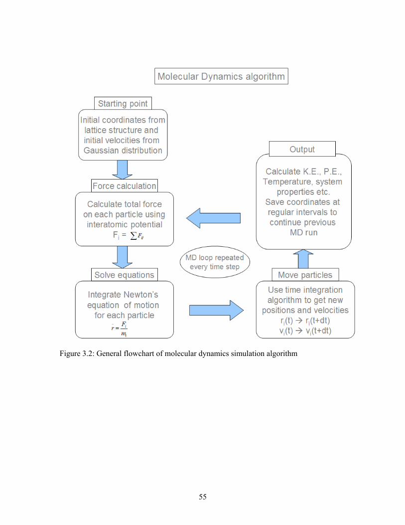
Figure 3.2: General flowchart of molecular dynamics simulation algorithm
55
Figure 3.2 shows a flowchart of molecular dynamics algorithm. Accuracy of a
molecular dynamics simulation is greatly affected by the choice of potential function
used to simulate the interaction between atoms. The potential is a function ( )ij ijrφ of the
interatomic distance between atoms i and j, representing the potential energy of the
system when the atoms are arranged in that specific configuration. This function is
usually constructed from the relative positions of the atoms with respect to each other,
rather than from the absolute positions. Forces on each atom are then derived as the
gradient of the potential with respect to the atomic displacements:
( )ijr ij ijijf rφ
→ →
= −∇ (3.3)
Thus we can describe a model in terms of force or the potential energy. Since
potential energy is a scalar quantity it is convenient to describe the model in terms of its
potential energy. In this work a nanofluid system is simulated using molecular dynamics
simulation. In this nanofluid system interaction between liquid-liquid, solid-solid and
liquid-solid molecules are considered. These interactions occur between the liquid
molecules, between the atoms of solid nanoparticle, and between the solid atoms and the
liquid molecules. These interactions have been simulated with 3 different interatomic
potentials, which are discussed later in this chapter. The electrostatic interaction between
the charged atoms of water has also been taken into account.
3.1.1 Potential Functions
The interaction potential used in a molecular dynamics simulation can be bonded
or non-bonded in nature. Most of non-bonded potentials are represented in terms of a pair
56

potential, which means the interactions between the atoms is considered as one pair at a
time. The simplest and most widely used pair-potential in molecular dynamics simulation
is Lennard-Jones [1924] or LJ potential. The molecular dynamics potential is a 12-6
potential which is attractive when the molecules are far apart and becomes strongly
repulsive when they come close together. Lennard-Jones potential has a r-6 attractive term
which represents the attractive van der Waals interaction between atom at large distances
and a r-12 repulsive term which becomes dominant when atoms come close to each other
this essentially represents the resistance to compression among atoms. For two atoms i
and j the Lennard-Jones pair potential is represented as:
12 6
( ) 4LJij ij
rr rσ σφ ε
⎡ ⎤⎛ ⎞ ⎛ ⎞⎢= −⎜ ⎟ ⎜ ⎟⎜ ⎟ ⎜ ⎟⎢ ⎥⎝ ⎠ ⎝ ⎠⎣ ⎦
⎥ (3.4)
Equation (3.4) gives the expression for the potential energy between an atom pair
interacting via the Lennard-Jones potential. Here, ε is the energy parameter which gives
the depth of the potential well, as shown in Figure 3.3, and σ is the length parameter, this
represents the interatomic distance at which the curve crosses the zero potential line.
These parameters are calculated by using quantum chemistry calculation or by curve-
fitting the experimental data. The r-12 part of the potential is the repulsive part of the force
and is dominant at small distances. As the two atoms come close to each other the
repulsive force increases rapidly and does not allow the atoms to form a bond. The r-6
part of the potential is the attractive part of the force and is dominant at relatively larger
interatomic distances. The resulting potential is shown in Figure 3.3.
57
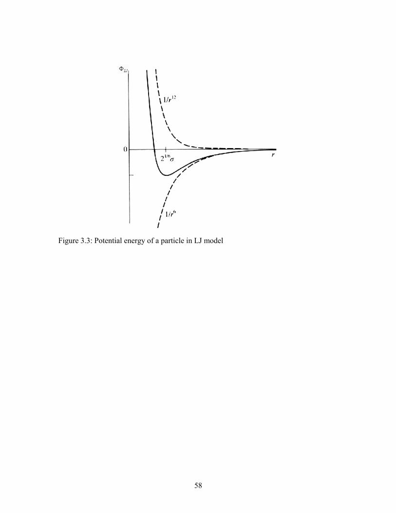
Figure 3.3: Potential energy of a particle in LJ model
58
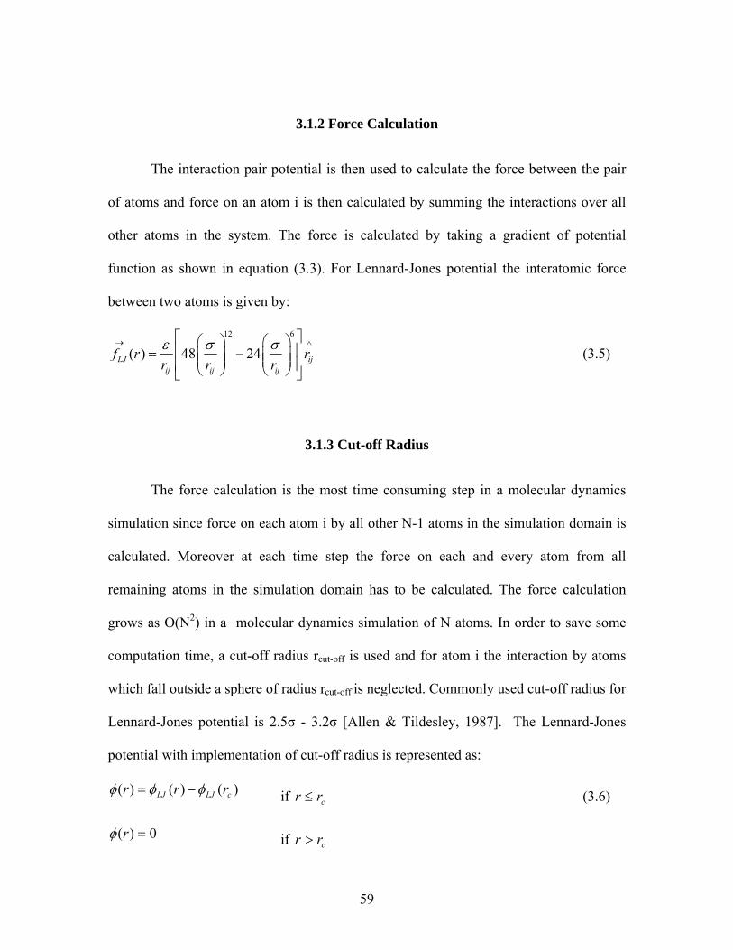
3.1.2 Force Calculation
The interaction pair potential is then used to calculate the force between the pair
of atoms and force on an atom i is then calculated by summing the interactions over all
other atoms in the system. The force is calculated by taking a gradient of potential
function as shown in equation (3.3). For Lennard-Jones potential the interatomic force
between two atoms is given by:
12 6
( ) 48 24LJ ijij ij ij
f rr r rε σ σ→ ∧⎡ ⎤⎛ ⎞ ⎛ ⎞⎢= −⎜ ⎟ ⎜ ⎟⎜ ⎟ ⎜ ⎟⎢ ⎥⎝ ⎠ ⎝ ⎠⎣ ⎦
r⎥ (3.5)
3.1.3 Cut-off Radius
The force calculation is the most time consuming step in a molecular dynamics
simulation since force on each atom i by all other N-1 atoms in the simulation domain is
calculated. Moreover at each time step the force on each and every atom from all
remaining atoms in the simulation domain has to be calculated. The force calculation
grows as O(N2) in a molecular dynamics simulation of N atoms. In order to save some
computation time, a cut-off radius rcut-off is used and for atom i the interaction by atoms
which fall outside a sphere of radius rcut-off is neglected. Commonly used cut-off radius for
Lennard-Jones potential is 2.5σ - 3.2σ [Allen & Tildesley, 1987]. The Lennard-Jones
potential with implementation of cut-off radius is represented as:
)()()( cLJLJ rrr φφφ −= if crr ≤ (3.6)
0)( =rφ if crr >
59
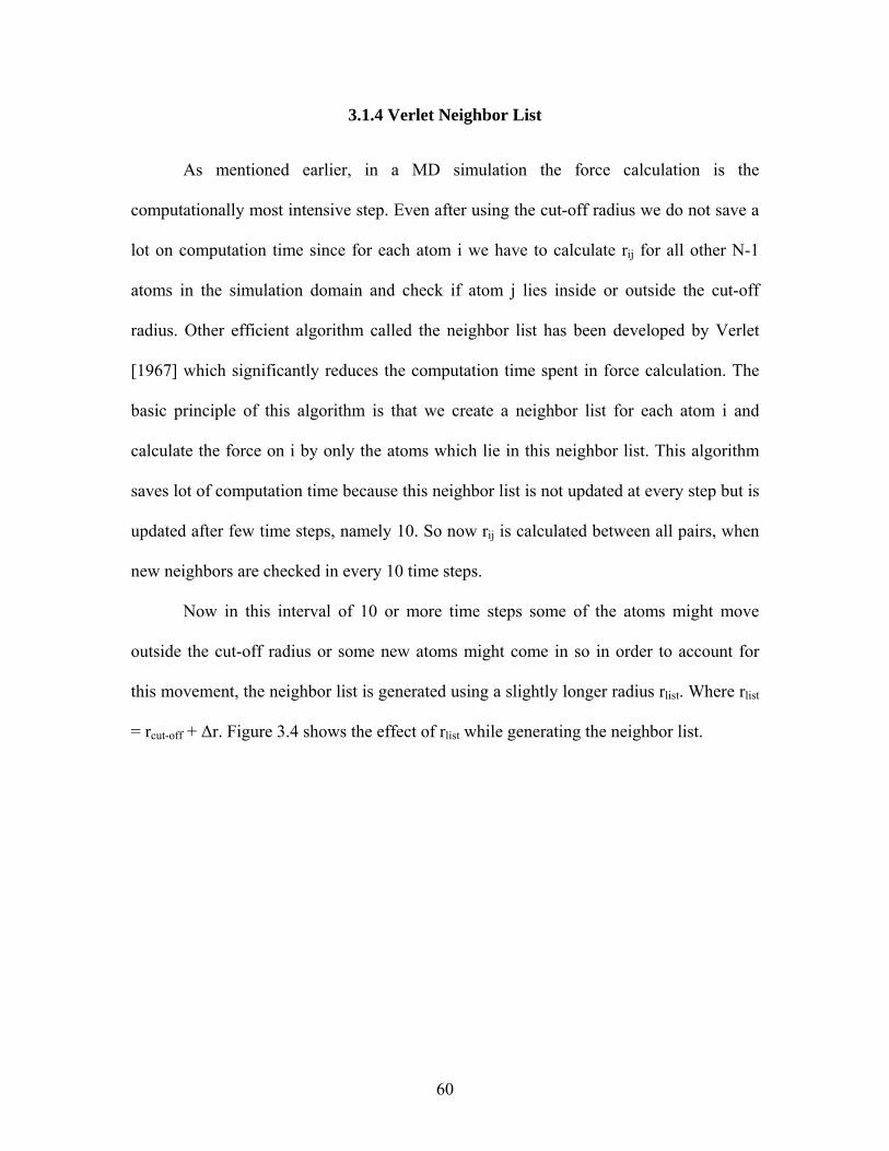
3.1.4 Verlet Neighbor List
As mentioned earlier, in a MD simulation the force calculation is the
computationally most intensive step. Even after using the cut-off radius we do not save a
lot on computation time since for each atom i we have to calculate rij for all other N-1
atoms in the simulation domain and check if atom j lies inside or outside the cut-off
radius. Other efficient algorithm called the neighbor list has been developed by Verlet
[1967] which significantly reduces the computation time spent in force calculation. The
basic principle of this algorithm is that we create a neighbor list for each atom i and
calculate the force on i by only the atoms which lie in this neighbor list. This algorithm
saves lot of computation time because this neighbor list is not updated at every step but is
updated after few time steps, namely 10. So now rij is calculated between all pairs, when
new neighbors are checked in every 10 time steps.
Now in this interval of 10 or more time steps some of the atoms might move
outside the cut-off radius or some new atoms might come in so in order to account for
this movement, the neighbor list is generated using a slightly longer radius rlist. Where rlist
= rcut-off + Δr. Figure 3.4 shows the effect of rlist while generating the neighbor list.
60
Figure 3.4: Neighbor-list construction with radius rlist
61
3.1.5 Integration of Equation of Motion
At every time step the force on every atom is calculated and then using Newton’s
law the acceleration of the particle is calculated. At each time step equation of motion for
every atom is then integrated numerically to find their velocities. The velocities are used
to advance the atoms and their new positions are calculated by numerically integrating
the velocities. The choice of numerical integration scheme is important in molecular
dynamics simulation, as it determines the stability of the system and also has an effect of
the energy conservation for the whole system. Verlet [1967] and predictor-corrector
[Allen & Tildesley, 1987] algorithms are commonly used for marching in time in a
molecular dynamics simulation. The basic idea behind the velocity Verlet algorithm is to
write one forward and one backward third-order Taylor series expansion of the position
r(t):
)()()6/1()()2/1()()()( 432 tOttbttattvtrttr Δ+Δ+Δ+Δ+=Δ+
)()()6/1()()2/1()()()( 432 tOttbttattvtrttr Δ+Δ−Δ+Δ−=Δ− (3.7)
Where v(t) is the velocity, a(t) is the acceleration and b(t) is the third derivative of
r with respect to t. Adding the two expressions we get:
)()()()(2)r(t 42 tOttattrtrt Δ+Δ+Δ−−=Δ+ (3.8)
This is the basic form of the Verlet algorithm, in which first we calculate r(t+Δt)
from r(t), r(t-Δt) and a(t) and then use r(t+Δt) and r(t-Δt) to calculate v(t). Now we can
calculate the velocities using the position as:
tttrttrtv
ΔΔ−−Δ+
=2
)()()( (3.9)
62
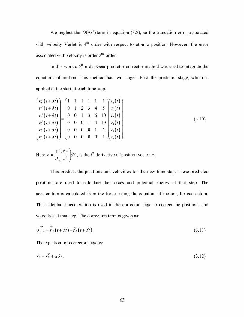
We neglect the term in equation (3.8), so the truncation error associated
with velocity Verlet is 4th order with respect to atomic position. However, the error
associated with velocity is order 2nd order.
4(O tΔ )
In this work a 5th order Gear predictor-corrector method was used to integrate the
equations of motion. This method has two stages. First the predictor stage, which is
applied at the start of each time step.
( )( )( )( )( )( )
( )( )( )( )( )( )
00
11
22
33
44
55
1 1 1 1 1 10 1 2 3 4 50 0 1 3 6 100 0 0 1 4 100 0 0 0 1 50 0 0 0 0 1
p
p
p
p
p
p
r tr t tr tr t tr tr t tr tr t tr tr t tr tr t t
δδδδδδ
⎛ ⎞ ⎛ ⎞+ ⎛ ⎞⎜ ⎟ ⎜ ⎟⎜ ⎟+⎜ ⎟ ⎜ ⎟⎜ ⎟⎜ ⎟ ⎜ ⎟⎜ ⎟+
=⎜ ⎟ ⎜⎜+⎜ ⎟ ⎜ ⎟⎜ ⎟
⎜ ⎟ ⎜ ⎟⎜ ⎟+⎜ ⎟ ⎜ ⎟⎜ ⎟⎜ ⎟⎜ ⎟⎜ ⎟+ ⎝ ⎠⎝ ⎠⎝ ⎠
⎟⎟ (3.10)
Here, 1!
ii
i i
rri t
tδ⎛ ⎞∂
= ⎜ ⎟∂⎝ ⎠
, is the ith derivative of position vector r ,
This predicts the positions and velocities for the new time step. These predicted
positions are used to calculate the forces and potential energy at that step. The
acceleration is calculated from the forces using the equation of motion, for each atom.
This calculated acceleration is used in the corrector stage to correct the positions and
velocities at that step. The correction term is given as:
( ) (2 2 2p
r r t t r t t )δ δ→ →
= + − +δ (3.11)
The equation for corrector stage is:
2c pn nr r rαδ= + (3.12)
63
Here,
3 /16251/ 360
111/181/ 61/ 60
α
⎛ ⎞⎜ ⎟⎜ ⎟⎜ ⎟
= ⎜ ⎟⎜ ⎟⎜ ⎟⎜ ⎟⎜ ⎟⎝ ⎠
These constants for the corrector stage are given by Gear. The corrected velocities
are used to calculate the kinetic energy, system temperature and other system properties.
Main motivation for using the predictor-corrector integrator is that the Gear algorithm has
very small energy fluctuations.
3.1.6 Periodic Boundary Condition
Periodic boundary condition (PBC) is used in almost all molecular dynamics
simulations where a wall is not encountered. The periodic boundary condition acts in a
way to simulate the bulk property of the system. In PBC each face of the cubic simulation
domain acts as a mirror and there is a mirror system on the other side of the boundary. So
every atom in the simulation domain actually represents infinite set of particles in the
replicated systems. All these “image” particles move together but are represented by only
a single atom in the actual simulation domain. Provided the interatomic forces are not
long-range we can consider that an atom only interacts with its nearest atom or image in
the periodic array. So every atom i in the simulation domain now interacts not only to the
atoms j in the simulation domain but also to the images in the surrounding boxes. If an
atom comes close to the boundary and then crosses it, it is re-inserted in the system from
the opposite boundary with same velocity. So the periodic boundary condition actually
makes sure that the number density of atoms in simulation domain and the momentum of
64
whole system is conserved. In molecular dynamics simulation, the periodic boundary
condition is applied in the following way:
xxx
xxx
xx
lrrlrr
rr
+=−=
= if (3.13)
0<><
x
xx
xx
rlrlr
Where rx is the x-coordinate of the atom i, lx is the length of the simulation
domain in x-direction. It is assumed that one of the vertices of the simulation domain is
the origin.
3.2 Molecular Simulation of Liquid Water
In this work the water molecules were modeled using molecular dynamics
simulations. The water molecule consists of two hydrogen atoms and one oxygen atom in
a tetrahedral bond structure. The angle between the two H-O bonds is 109.47˚, as shown
in Figure 3.5.
The water molecule has a bond length, 0.1H Or − nm= and the angle
°= 47.109HOHθ with charges directly on oxygen and hydrogen atoms. It takes charge on
oxygen and hydrogen atoms equal to δ- = –0.820e and δ+ = +0.410e, respectively. Here,
e, is the electronic charge. There are various interactions that occur between the atoms in
a water molecule and between a pair of water molecules. The H-O bond can stretch or the
H-O-H bond angle can change causing bond bending in the molecule.
65

Figure 3.5: Structure of water molecule
66
In a pair of water molecules, the oxygen atoms belonging to two molecules can
exert force on each other, or the hydrogen atom of one molecule can exert force on
hydrogen atom of other molecule, or on the oxygen atom of other molecule. There can
also be H+ or O-2 ions in water, which will interact with each other via the coulombic
interaction.
In earlier studies simplifications have been made and the complex water molecule
has been replaced with a single “LJ atom” and the various interactions mentioned above
have been modeled using the famous LJ potential, because of its simplicity and also
because it required low computational resources. In this approach the bi-polar nature of
the water molecules is lost and it interacts with another molecule via only the van der
Waals forces. Although this approach is simple to implement and requires very low
computational resources, this simplicity comes at the cost of accuracy of results. The LJ
water model is not able to reproduce the properties like diffusion coefficient, radial
distribution function, and thermal conductivity of water as measured in real experiments.
To accurately predict the structural and thermodynamic properties of water and
compare them well with the experimental data, all the complicated bonded and non-
bonded interactions have to be taken into account in the model. Several models for water
molecule have been proposed in the past such as SPC (simple point charge) model
[Berendsen et al, 1981], TIPS model [Jorgensen, 1981] and TIPS2 [Jorgensen, 1982].
Berendsen et al, [1987] reparametrized the SPC model to obtain correct energy and better
matching density and called it SPC/E (simple point charge extended) model. These
potentials model the water molecule as 3 site, 4 site or 5 site models. In the 3 site model,
the charge on individual hydrogen and oxygen atoms are kept on the atoms itself. In the
67
4- and 5-site models, the charge is kept at a distance from the atoms’ locations. These
models predict the structural and thermodynamic properties of water with varying degree
of accuracy. The SPC/E model has been tested and used by many researchers to model
water molecules in the past. Although these potentials compare well with experiments,
they model the H-O bonds as rigid bonds and restrict the ‘bond-stretching’ and ‘bond-
bending’ mechanisms in a water molecule.
3.3 Potential Functions Used in This Work
In a conventional sense, molecular dynamics uses interatomic potentials derived
based on ab initio calculations. From these potentials the interaction force between
atoms, the kinetic and potential energies of atoms are calculated. As a result the accuracy
and validity of the MD simulation are dependent on the potential functions used. In order
to accurately simulate the nanofluid system under consideration all possible atomic
interactions have been considered. In this simulation interaction between liquid-liquid,
solid-solid and liquid-solid atoms along with the coulombic interaction between charged
particles are taken into account. This chapter discusses all the potential functions used in
this work.
3.3.1 Liquid-Liquid Interaction
Levitt et al [1997] proposed a model for water that consists of 3 atomic sites,
corresponding to H, O, and H atoms, with flexible bonds to mimic the real behavior of
the water molecule. This model is called the Flexible 3 Center (F3C) model. In this
model the flexible nature of H-O bonds and the bi-polar nature of water molecule are
68
kept intact. The F3C model represents the H-O bond stretching and H-O-H bond bending
in water molecule as spring forces. Various atomic pairs between two water molecules
(H1-H2, H1-O2, O1-O2) interact with each other via a Lennard-Jones type 12-6 potential.
Here, the subscripts represent water molecule 1 and 2. The ionic pairs between 2
molecules (H1+-H2
+, H1+-O2
-2, O1-2-O2
-2) interact with each other via the coulombic or
electrostatic interaction. The following expressions are used for the various interactions
mentioned above:
• Interaction potential for H-O bond stretching:
( 20b i
iK b bφ = −∑ )
)
(3.14)
Here, b0 is the original H-O bond length, and Kb is the spring constant for the H-O
bond stretching.
• Interaction potential for H-O-H bond bending:
( 20i
iKθφ θ θ= −∑ (3.15)
Here, θ0 is the original H-O-H bond angle, and Kθ is the spring constant for the H-O-H
bond bending.
• Non-bonded interaction between a pair of atoms i, j:
( )12 6
2o ovdw ij
ij ij
r r S rr r
φ ε ε⎡ ⎤⎛ ⎞ ⎛ ⎞⎢= − −⎜ ⎟ ⎜ ⎟⎜ ⎟ ⎜ ⎟⎢ ⎥⎝ ⎠ ⎝ ⎠⎣ ⎦
∑ ⎥ (3.16)
Here, ε is the energy parameter for the i, j atom pair, ro is the length parameter for the i, j
atom pair, and Svdw is the first order truncation function.
• Non-bonded electrostatic interaction between a pair of atoms i, j:
69
14
i jels
o ij
q qS
rφ
πε⎡ ⎤
= ⎢⎢ ⎥⎣ ⎦
∑ − ⎥ (3.17)
Here, εo is the electric constant, and qi and qj are the charges on the atoms i, and j and rc is
the cut-off radius.
For the LJ and coulombic potentials, only the atom pairs falling inside a specified
cut-off distance are accounted for while calculating the forces. As seen in Figure 3.1 the
potential energy for LJ potential almost goes to zero at a distance greater than 2.5σ. So
any atoms falling outside this distance will not contribute much towards the force and
potential calculation. This cut-off approach reduces the number of force & potential
energy calculations thereby reducing the computational load. The first order truncation
shift function, S(t), is used to implement the cut-off radius in the simulation. S(t) is given
as:
( ) ( ) ( ) ( ) , ,
0
cc c
fc
df rcf r r r for r
S r drr
for r r
⎧ ⎡ ⎤+ − <⎪ ⎢ ⎥= ⎨ ⎣ ⎦ ≥⎪
⎩
(3.18)
So the cut-off part of LJ type potential Svdw is given as:
( )12 6 12 6
12( )2o o c ovdw
c c c c
r r r r r rS rr r r r r
ε ε ε ε⎡ ⎤ ⎡⎛ ⎞ ⎛ ⎞ ⎛ ⎞ ⎛ ⎞−⎢ ⎥ ⎢= − − −⎜ ⎟ ⎜ ⎟ ⎜ ⎟ ⎜ ⎟⎢ ⎥ ⎢⎝ ⎠ ⎝ ⎠ ⎝ ⎠ ⎝ ⎠⎣ ⎦ ⎣
o
c
⎤⎥⎥⎦
(3.19)
And, the cut-off part of the coulombic potential Sele is given as:
( ) ( )14
i j i jcels
o c c c
q q q qr rS r
r r rπε⎡ ⎤− ⎛ ⎞
= −⎢ ⎜ ⎟⎢ ⎥⎝ ⎠⎣ ⎦
⎥ (3.20)
Levitt et al [1997] calculated various structural and thermodynamic properties of
water using the F3C model and compared them with properties calculated from other
water models and with experimental data. They calculated the potential energy, specific
70
heat at constant volume (Cv), diffusion coefficient, mean-square distance between oxygen
atoms, and the radial distribution function for water at 298 ˚K temperature. Good
agreement was found when this data was compared with other models and experiments.
In this work the F3C model was used to simulate water and calculate its thermal
conductivity. This work will also prove as a validation for further work in which water is
used as a base fluid for a nanofluid system.
To start a molecular dynamics simulation, initial coordinates and velocities of
each water molecule are required. The molecular dynamics simulation was started with
tetrahedral, bi-polar, water molecules placed in a simple cubic lattice. This initial
structure was chosen to keep symmetry in the system. The initial velocities were
calculated using the kinetic theory of gases. According to the kinetic theory each atom
has 12 BK T kinetic energy along each degree of freedom. Here, KB is the Boltzmann
constant, and T is the temperature of the system. For a monoatomic system there are 3
degrees of freedom from the translational motion. So, a system of N atoms will have total
of 32 BNK T kinetic energy.
2
1
1 3 2 2
N
i i Bi
KE m v NK T=
= =∑ (3.21)
In the flexible water molecule, since the bonds are not rigid, each atom can move
independently in the x, y, and z directions (while still forming the bonds in the water
molecule) and hence has 3 degrees of freedom. For 3 atoms total degrees of freedom in
every water molecule then become 9. If we consider the motion of water molecule as a
whole, it has 3 translational degrees of freedom, 3 rotational degrees of freedom, and 3
vibrational (2 bond-stretching and 1 bond-bending) degrees of freedom. So a total of 9
71

degrees of freedom are there in the water molecule. The flexible water model mimics the
behavior of a real water molecule by letting each atom move individually. This flexible
nature of the bonds also simulates the rotational motion of the water molecule.
In a rigid water model, e.g. SPC/E, the 3 vibration degrees of freedom are not
accounted for. Also the rotation of molecules adds more complication to the
computational procedure. The rotational motion is simplified in flexible water model as it
comes out of the individual motion of the atoms in the molecules.
3.3.2 Interactions in Solid Nanoparticle
The choice of interaction potential for the solid nanoparticle in this work reflects
the need for an economic, insightful analysis with reasonable accuracy. The complex
chemical reactions between the surface atoms of a nanoparticle and the liquid molecules
have not yet been identified in the experimental research. To identify these chemical
reactions quantum-chemistry models like Carr-Parrinello Molecular Dynamics (CPMD)
or Density Functional Theory (DFT) are required. In this work we wish to study general
water based nanofluid system, rather than a specific nanofluid like alumina-water. So a
simple two body Lennard-Jones potential is used to model the solid nanoparticle. The
solid nanoparticle in this simulation consists of Lennard-Jones atoms in a FCC lattice.
Each atom in the nanoparticle is connected to its first neighbors by finite extensible
nonlinear elastic (FENE) bonding potential [Vladkov & Barrat, 2006] as shown in
equation (3.22).
72
22 ln 1 ,
2 o
ijFENE ij o
o
rk R r RR
φ⎡ ⎤⎛ ⎞⎢ ⎥= − ⎜ ⎟⎢ ⎥⎝ ⎠⎣ ⎦
<
(3.22)
Here, 1.5oR σ= , and 230.0k εσ
= .
The atoms in this solid particle vibrate around their mean position and simulate
the phonon mode of heat transport as seen in solids. This model nanoparticle will closely
simulate a non-metallic particle like oxides, where the thermal conductivity arises from
the phonon mode and not from electrons as in the case of metals. The Lennard-Jones
parameters for copper, as used by Sarkar & Selvam [2007] and Li et al [2008] are used
for the solid nanoparticle. The primary focus this thesis is to predict the qualitative trends
of thermal conductivity enhancement and study various mechanisms causing the higher
thermal transport in nanofluids using molecular dynamic simulation and not to capture
the complex chemical reactions between these atoms.
3.3.3 Interaction between Solid-Liquid Atoms
The third important potential to establish is the interfacial potential between the
atoms in solid nanoparticle and the liquid molecules. The pairwise Lennard-Jones
potential is used to model the interaction between atoms of solid nanoparticle and atoms
in liquid water. To determine the parameters for the solid-liquid interaction, the Lorentz-
Berthelot mixing rule [Allen & Tildesley, 1987] is used:
2ss l
sllσ σσ +
=
and
73
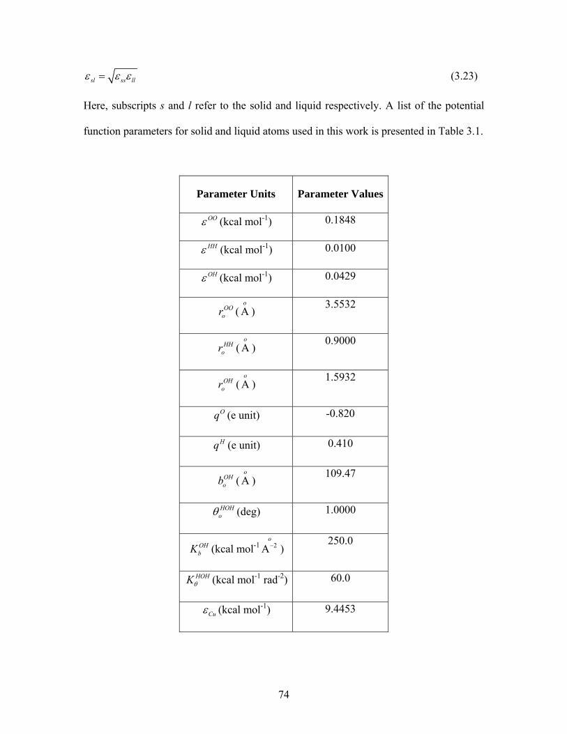
sl ss llε ε ε= (3.23)
Here, subscripts s and l refer to the solid and liquid respectively. A list of the potential
function parameters for solid and liquid atoms used in this work is presented in Table 3.1.
Parameter Units Parameter Values
OOε (kcal mol-1) 0.1848
HHε (kcal mol-1) 0.0100
OHε (kcal mol-1) 0.0429
OOor ( A )
o 3.5532
HHor ( ) A
o 0.9000
OHor ( ) A
o 1.5932
Oq (e unit) -0.820
Hq (e unit) 0.410
OHob ( ) A
o 109.47
HOHoθ (deg) 1.0000
OHbK (kcal mol-1 2A
o− )
250.0
HOHKθ (kcal mol-1 rad-2) 60.0
Cuε (kcal mol-1) 9.4453
74
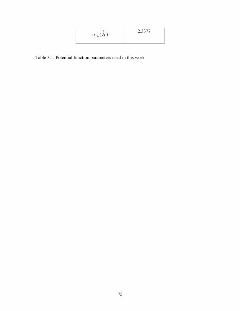
) 2.3377
Cuσ ( Ao
Table 3.1: Potential function parameters used in this work
75
3.3.4 Coulombic Interaction
Till now various pair potential functions used in this simulation have been
discussed here. These interactions are essentially short-ranged in nature, which means
that the potential decreases quickly as the distance between a pair of atoms increases and
we can use a cut-off radius to ignore the interactions with interatomic distance larger than
the cut-off radius. Short-range interactions exclude a very important group of interactions
involving electric charges and dipoles. In this system even though individual water
molecules are electrically neutral but individual oxygen and hydrogen carry negative and
positive charges respectively, similarly the silica nanoparticle as a whole does not carry
any charge but oxygen and silicon atoms carry negative and positive charges
respectively. The interactions between electric charges are long-ranged in nature, which
means that the force between charges does not decay even at large distances, so it can not
be truncated and the interactions over the whole simulation domain should be considered.
The electronic interaction between charge-charge decays as rij-1 and the interaction
between dipole-dipole decays as rij-3. So these interactions do not decay fast even at large
distances. A spherical truncation using a cut-off radius can not be done here because the
resulting sphere around a given charge could be charged (i.e. sum of all charges in the
spherical domain might not be zero). Also the charges moving in and out of this spherical
domain would create artificial surface effects at r=rc. The electronic interactions or
coulombic interactions essentially require O(N2) computational time. Even with modern
high speed computers this high computational cost is a serious problem in MD
simulations with thousands of atoms.
76
In this simulation an approximate method called Wolf method [Wolf et al, 1999]
is used to simulate the coulombic interactions between charged atoms. The Wolf method
was conceptualized on the fact that ionic systems have a tendency to be locally charge
neutral, i.e. the ions arrange themselves in such a way that each charge is surrounded by
neighboring charges of opposite sign, thereby creating a locally charge neutral zone. This
kind of behavior is called “screening” of ions and is observed in molten salts, ionic gases,
ionic solutions and metallic conductors. It has been shown both theoretically [Evjen,
1932] and numerically [Clarke et al, 1984, Woodcock, 1975, Wolf 1992] that the
effective coulombic interaction in condensed systems are actually short-ranged. It has
also been suggested that at long range there is almost complete cancellation of coulombic
effects. Based on these findings, Wolf et al [1999] proposed an exact method for
simulation of coulombic system by spherically truncated, pairwise 1/r summation. Wolf
method is suited for this simulation since there are no ions in the simulation domain,
individual atoms carry certain charge but the molecules as a whole are locally charge
neutral.
This method sums the total potential energy over all the atomic sites in the system
and solves iteratively the self-consistent equations for the induced dipoles at each step of
the molecular dynamics. Since we are using a truncated potential the following term is
added to the total potential energy of the system to consider the effect of interaction
between charges which are at an interatomic distance greater than the cut-off radius.
∑−=k
kkpol EU μ21 (3.24)
77
Where, Ek is the electric field at the location of site k due to all the fixed charges
in the system and μk is the induced dipole moment vector at location k. The induced
dipoles are determined by iteratively solving the equation:
⎥⎦
⎤⎢⎣
⎡⋅−= ∑
≠lklklkkk TE μαμ (3.25)
Here αk is the atomic polarizability assigned to site k, and Tkl is the dipole–dipole
tensor. In the above approach, one needs to readjust the positions of the charges for each
atom, and to assign atomic polarizability to each atom without changing the form of each
potential expression. The electrostatic interactions between charges qi and qj are then
modeled using the following approximation:
ji
jiji
ji
ji
rrerfqq
rqq
,
,
,
)(α×= (3.26)
The advantage of the Wolf method over the traditional Ewald sum method [Allen
& Tildesley, 1987] is that it can significantly reduce the required computational time. The
Wolf method is essentially equivalent to ignoring the long range electrostatic interactions
in the Ewald sum method. Even though Wolf method ignores the long-range interaction
but it is successful because it forces the net charge to be zero in the spherical volume
confined by the cut-off radius. The parameter α in Eq. (3.19) provides the damping
necessary to make the electrostatic interaction short range. Demontis et al [2001] propose
a value of 4/L for α, where L is the length of simulation domain. They also show that this
value gives good agreement with the Ewald sum method. For the current simulation, two
constant values of 0.25 and 0.07 are chosen for silica and water respectively.
78
3.3 Generation of Nanoparticle
In order to establish a reliable molecular dynamics model initial coordinates of the
atoms in the solid nanoparticle are required. A crystallographic-based coordinate system
is necessary to get the position of each atom in the nanoparticle. Before building a lattice
structure, the primitive vector should be obtained and a unit cell of the crystal is created.
The unit cell is then replicated in x, y, and z directions to create a bulk crystal structure.
For this work the solid nanoparticle was prepared by creating the bulk copper crystal in a
FCC arrangement and then carving out a spherical nanoparticle of desired diameter from
this bulk crystal. The atoms within the sphere were linked to their first neighbors by the
FENE bond. Figure 3.6 shows the FCC unit cell, 1 nm and 2 nm nanoparticle structure
used in the simulation.
79
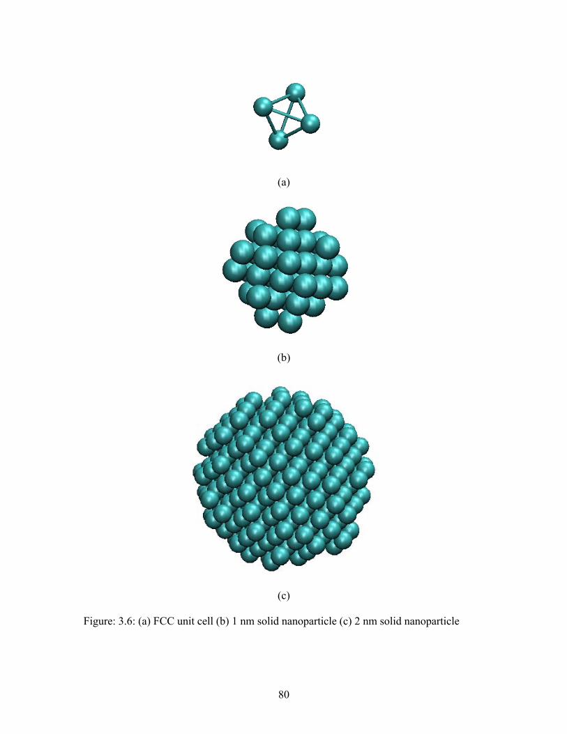
(a)
(b)
(c)
Figure: 3.6: (a) FCC unit cell (b) 1 nm solid nanoparticle (c) 2 nm solid nanoparticle
80
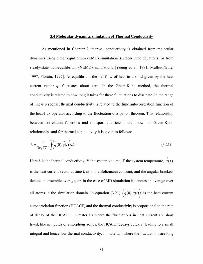
3.4 Molecular dynamics simulation of Thermal Conductivity
As mentioned in Chapter 2, thermal conductivity is obtained from molecular
dynamics using either equilibrium (EMD) simulations (Green-Kubo equations) or from
steady-state non-equilibrium (NEMD) simulations [Young et al, 1991, Muller-Plathe,
1997, Florain, 1997]. At equilibrium the net flow of heat in a solid given by the heat
current vector q, fluctuates about zero. In the Green-Kubo method, the thermal
conductivity is related to how long it takes for these fluctuations to dissipate. In the range
of linear response, thermal conductivity is related to the time autocorrelation function of
the heat-flux operator according to the fluctuation-dissipation theorem. This relationship
between correlation functions and transport coefficients are known as Green-Kubo
relationships and for thermal conductivity it is given as follows:
20
1 (0). ( )3 B
q q t dk VT
λ∞ → →
= ∫ t (3.21)
Here λ is the thermal conductivity, V the system volume, T the system temperature,
is the heat current vector at time t, kB is the Boltzmann constant, and the angular brackets
denote an ensemble average, or, in the case of MD simulation it denotes an average over
all atoms in the simulation domain. In equation (3.21)
( )q t→
(0). ( )q q t→ →
is the heat current
autocorrelation function (HCACF) and the thermal conductivity is proportional to the rate
of decay of the HCACF. In materials where the fluctuations in heat current are short
lived, like in liquids or amorphous solids, the HCACF decays quickly, leading to a small
integral and hence low thermal conductivity. In materials where the fluctuations are long
81
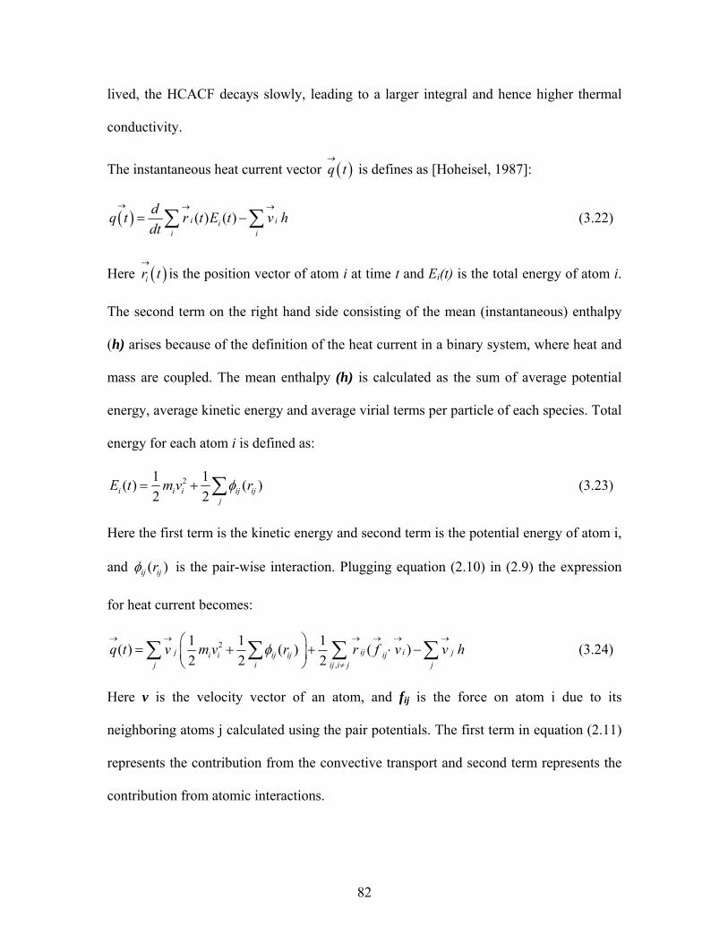
lived, the HCACF decays slowly, leading to a larger integral and hence higher thermal
conductivity.
The instantaneous heat current vector is defines as [Hoheisel, 1987]: ( )q t→
( ) ( ) ( )i iii i
dq t r t E t v hdt
→ → →
= −∑ ∑ (3.22)
Here is the position vector of atom i at time t and Ei(t) is the total energy of atom i.
The second term on the right hand side consisting of the mean (instantaneous) enthalpy
(h) arises because of the definition of the heat current in a binary system, where heat and
mass are coupled. The mean enthalpy (h) is calculated as the sum of average potential
energy, average kinetic energy and average virial terms per particle of each species. Total
energy for each atom i is defined as:
( )ir t→
21 1( ) ( )2 2i i i ij
j
E t m v rφ= + ∑ ij (3.23)
Here the first term is the kinetic energy and second term is the potential energy of atom i,
and ( )ij ijrφ is the pair-wise interaction. Plugging equation (2.10) in (2.9) the expression
for heat current becomes:
2
,
1 1 1( ) ( ) ( )2 2 2
ijj ii i ij ij ijj i ij i j
q t v m v r r f v v hφ→ → → → → →
≠
⎛ ⎞= + + ⋅ −⎜ ⎟
⎝ ⎠∑ ∑ ∑ j
j∑ (3.24)
Here v is the velocity vector of an atom, and fij is the force on atom i due to its
neighboring atoms j calculated using the pair potentials. The first term in equation (2.11)
represents the contribution from the convective transport and second term represents the
contribution from atomic interactions.
82

As mentioned earlier one major advantage of Green-Kubo method over the
NEMD method is that complete anisotropic thermal conductivity of the system can be
calculated in one simulation. While in the case of direct method or NEMD, 3 separate
simulations need to be run to calculate conductivity in 3 directions. In the NEMD
simulation, extreme temperature gradients (1010 ˚K/m) are encountered, due to the small
simulation domain size, which can adversely affect the dynamics at the solid-liquid
interface. So in this work the equilibrium molecular dynamic simulation with Green-
Kubo correlation is used to calculate the thermal conductivity of nanofluids. The Green-
Kubo approach has been used to calculate thermal conductivity of LJ argon [Vogelsang
et al 1987, Kaburaki et al 1999], diamond [Che et al 2000], silicon [Volz & Chen 2000]
and nanofluids [Keblinski et al 2002, Eapen et al 2007, Sarkar & Selvam 2007].
83
CHAPTER FOUR: VALIDATION OF THE MD CODE
In any computer simulation work it is necessary to validate the model with some
well known experimental results or with other simulation work published in the literature.
In this work two main potential functions, (1) Lennard-Jones potential, and (2) F3C
model for water, were used with the Green-Kubo correlation to calculate the thermal
conductivity of the nanofluid system. Before presenting the results for the nanofluid
system, it is necessary to validate the code for both of these models. The molecular
dynamics code developed in this work is separately validated for the Lennard-Jones
potential and F3C model.
4.1 Validation of Lennard-Jones based MD code
Lennard-Jones potential was first developed to model rare gases like Argon etc.
[Rahman, 1964]. Lennard-Jones potential has been proven to be reliable in predicting the
static and dynamic properties of both solid and liquid Argon [Vogelsang et al 1987,
Kaburaki et al 1999, Tretiakov & Scandolo 2004]. The Lennard-Jones potential
parameters that best reproduce the thermodynamics of Argon are ε = 1.67 x 10⁻²¹ J, and σ
= 3.405 Angstrom [Allen & Tildesley, 1987]. To validate the molecular dynamics code
and the application of Green-Kubo correlation, the thermal conductivity of liquid Argon
is calculated and compared with the thermal conductivity calculated by Vogelsang et al
[1987]. The thermal conductivity was calculated for state point 1, defined in Vogelsang et
al [1987] by the dimensionless temperature and number density as T* = 0.73 and ρ* =
0.8442. The dimensionless temperature and density are given as:
84
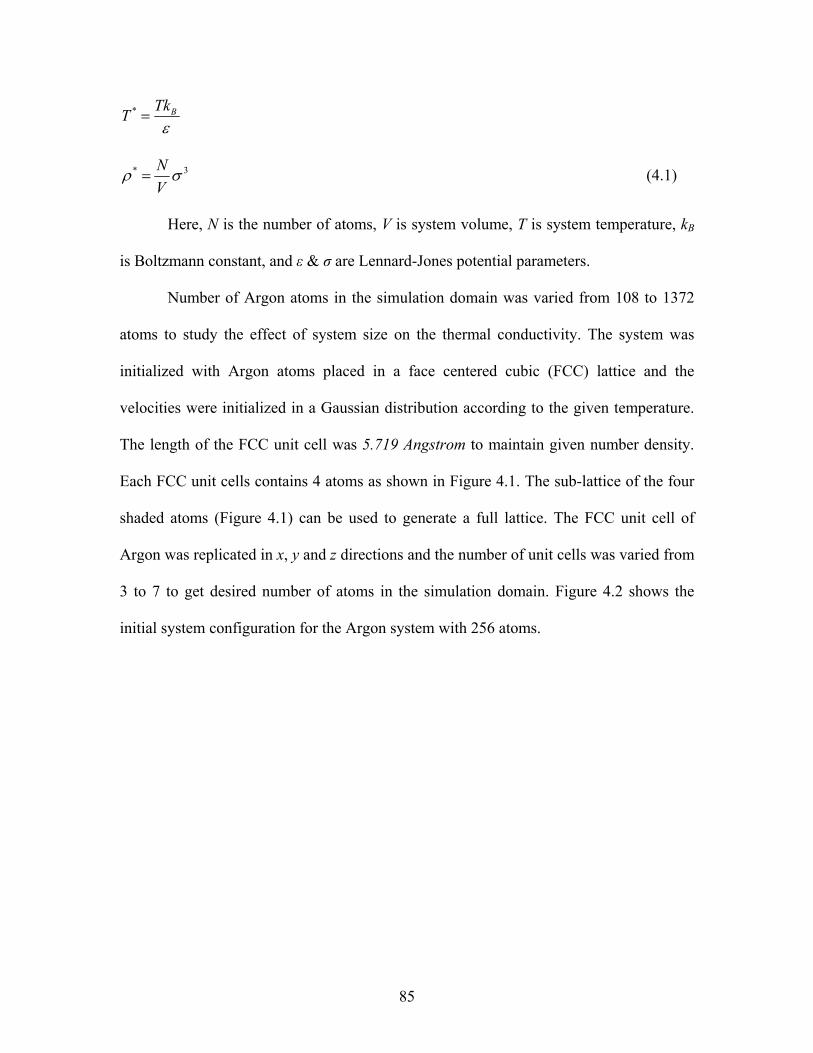
* BTkTε
=
* NV
3ρ σ= (4.1)
Here, N is the number of atoms, V is system volume, T is system temperature, kB
is Boltzmann constant, and ε & σ are Lennard-Jones potential parameters.
Number of Argon atoms in the simulation domain was varied from 108 to 1372
atoms to study the effect of system size on the thermal conductivity. The system was
initialized with Argon atoms placed in a face centered cubic (FCC) lattice and the
velocities were initialized in a Gaussian distribution according to the given temperature.
The length of the FCC unit cell was 5.719 Angstrom to maintain given number density.
Each FCC unit cells contains 4 atoms as shown in Figure 4.1. The sub-lattice of the four
shaded atoms (Figure 4.1) can be used to generate a full lattice. The FCC unit cell of
Argon was replicated in x, y and z directions and the number of unit cells was varied from
3 to 7 to get desired number of atoms in the simulation domain. Figure 4.2 shows the
initial system configuration for the Argon system with 256 atoms.
85
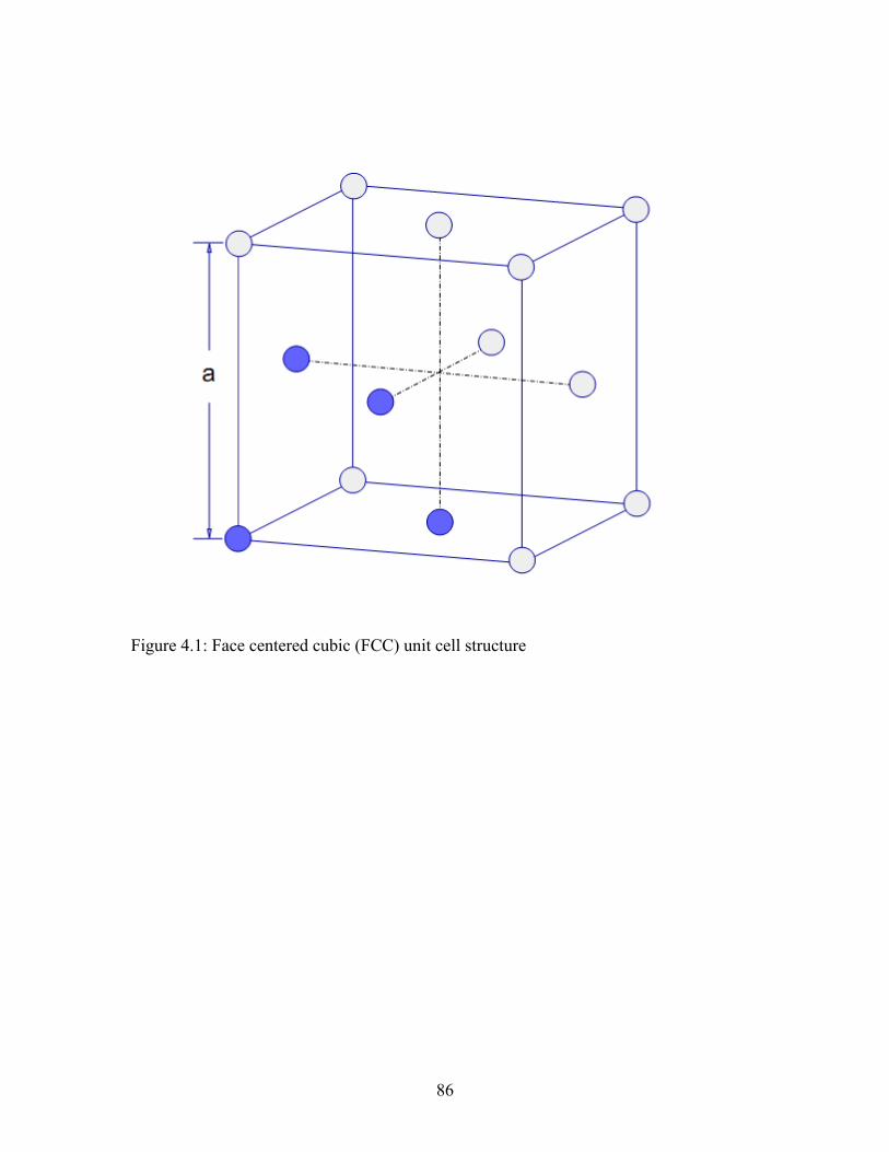
Figure 4.1: Face centered cubic (FCC) unit cell structure
86
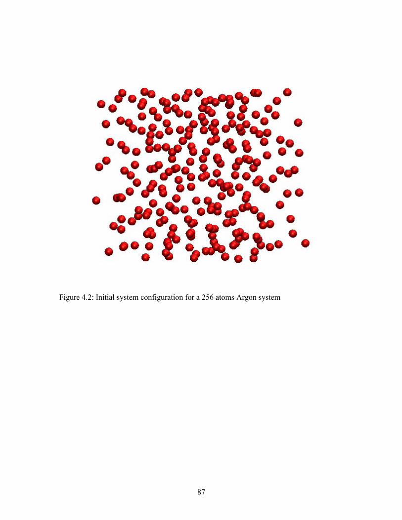
Figure 4.2: Initial system configuration for a 256 atoms Argon system
87
After initializing the system in FCC lattice and with a Gaussian velocity
distribution corresponding to the given temperature the system was equilibrated in NVT
ensemble for 5x10⁵ time steps. In the NVT ensemble, number of atoms, volume of the
simulation domain and the system temperature are kept constant. Velocity scaling method
was used to keep the temperature constant in the equilibration period. A time step of 0.01
picoseconds was used for the simulation and was found to be sufficient to resolve the
phenomenon under consideration. Velocity verlet [Verlet, 1968] algorithm was used to
integrate the equations of motion. Atomic interactions were truncated and shifted at a cut-
off radius of 2.5σ. After first 5x10⁵ steps equilibration period was over, temperature
constraint from the system was removed and the system was allowed to evolve in the
NVE ensemble for 106 time steps. The heat current was calculated in this period and
Green-Kubo correlation with a correlation length of 5x10⁴ time steps was used to
calculate the integral of the heat current autocorrelation function. Thermal conductivity of
various systems was calculated and is compared with the values published by Vogelsang
et al [1987] in Table 4.1 and Figure 4.3. It is observed that the thermal conductivity value
calculated by our molecular dynamics code is in good agreement with the values
published in the literature for the given temperature and density.
88
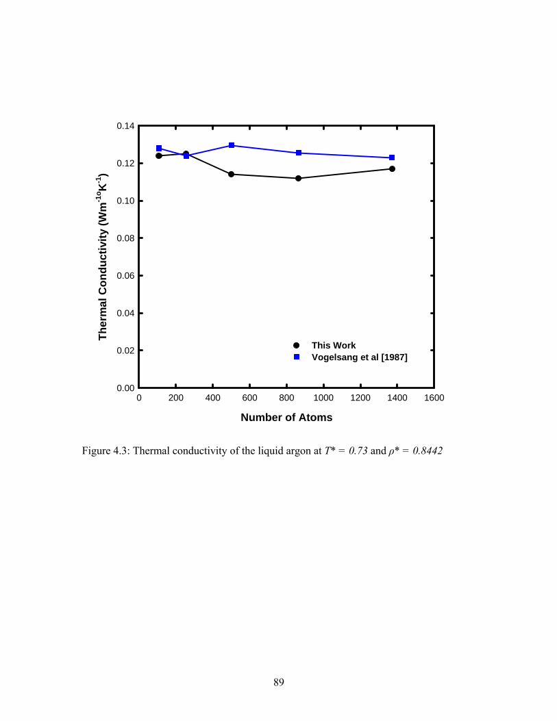
Number of Atoms
0 200 400 600 800 1000 1200 1400 1600
Ther
mal
Con
duct
ivity
(Wm
-1o K
-1)
0.00
0.02
0.04
0.06
0.08
0.10
0.12
0.14
This WorkVogelsang et al [1987]
Figure 4.3: Thermal conductivity of the liquid argon at T* = 0.73 and ρ* = 0.8442
89
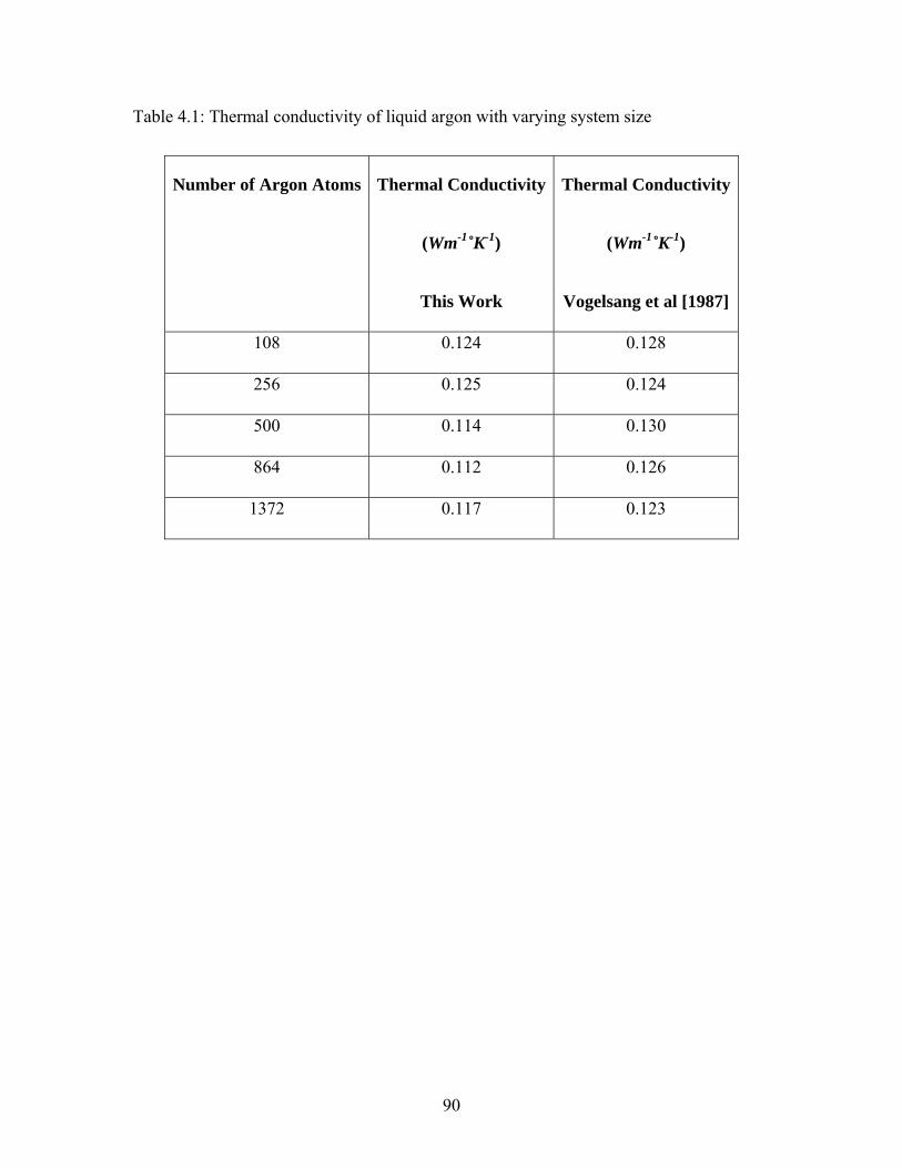
Table 4.1: Thermal conductivity of liquid argon with varying system size
Number of Argon Atoms Thermal Conductivity
(Wm-1˚K-1)
This Work
Thermal Conductivity
(Wm-1˚K-1)
Vogelsang et al [1987]
108 0.124 0.128
256 0.125 0.124
500 0.114 0.130
864 0.112 0.126
1372 0.117 0.123
90
4.1 Validation of F3C water model
A molecular dynamics code implementing the F3C (flexible 3 center) model for
water was developed for this work. The F3C model has been proven to predict various
thermodynamic properties of water like potential energy and specific heat at constant
volume, kinetic properties like the diffusion coefficient and structural properties like the
radial distribution function of oxygen in water [Levitt et al 1997]. But this model has
never been used to calculate the thermal conductivity of water, so it is even more
important to validate the model before using it to calculate the thermal conductivity of the
nanofluid system. Number of water molecules was varied to study the effect of
simulation domain size (or the number of water molecules) on the thermal conductivity
of water. 216, 343, 512, 729 and 1000 water molecules were used in a series of
simulation at 300 ˚K temperature and 1 atm. pressure. Simulation domain size was
changed from 18.62 Angstrom to 31.03 Angstrom in order to keep the density of water
constant at 1 gm/cm3. Water molecules were initialized in a simple cubic lattice to avoid
overlap of molecular positions which could happen in a random placement of molecules.
The size of the simulation domain was increased with the number of simple cubic unit
cells in all three directions form 6 to 10 unit cells. The size of the unit cell to maintain a
density of 1 gm/cm3 was 3.1036 Angstrom. A time step of 0.1 fs was used in all
simulations. The system was equilibrated in the NVT ensemble for 5x10⁵ time steps. In
the equilibration period the system temperature was kept constant using the velocity
scaling method. After the equilibration period, the temperature constraint was removed
and system was allowed to evolve in the NVE ensemble. The heat current was calculated
91
and the Green-Kubo correlation was used to calculate the thermal conductivity of the
water only system.
Figure 4.4 shows the initial system configuration for a 500 molecule water
system. Figure 4.5 shows the thermal conductivity values for various cases, the values are
also presented in Table 4.2. It was observed that the calculated thermal conductivity of
the F3C water system fluctuates around the experimentally measured value of 0.61
at 300 ˚K and 1 atm. pressure. 1Wm K− −° 1
92
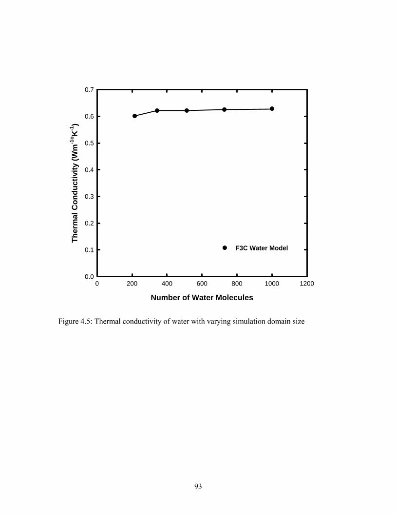
Number of Water Molecules
0 200 400 600 800 1000 1200
Ther
mal
Con
duct
ivity
(Wm
-1o K
-1)
0.0
0.1
0.2
0.3
0.4
0.5
0.6
0.7
F3C Water Model
Figure 4.5: Thermal conductivity of water with varying simulation domain size
93
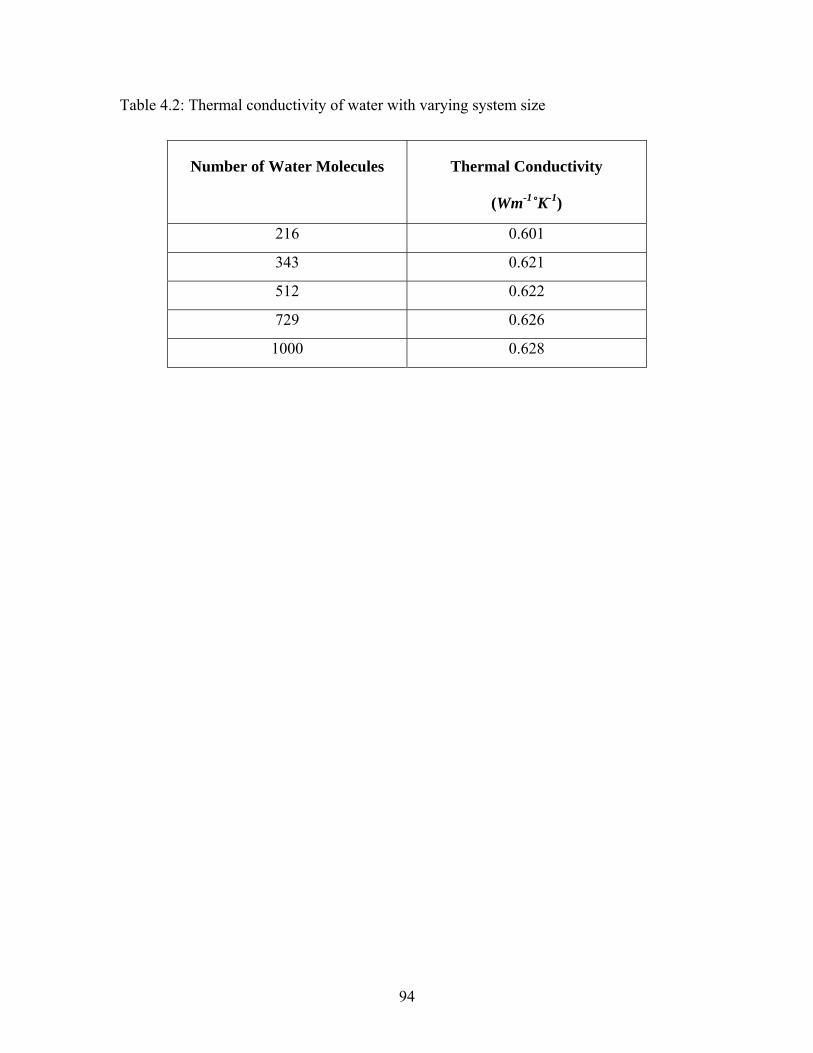
Table 4.2: Thermal conductivity of water with varying system size
Number of Water Molecules Thermal Conductivity
(Wm-1˚K-1)
216 0.601
343 0.621
512 0.622
729 0.626
1000 0.628
94
Although the calculated thermal conductivity is approximately 3% higher
compared to experimental value of 0.61 W/m-K, it is well within the acceptable
numerical error range of 5%, which could arise from truncation error or from the model
potential function itself.
Figure 4.6, shows the variation of thermal conductivity vs. correlation length as
calculated from the Green-Kubo correlation for 512 and 1000 molecule runs. The
correlation length is the number of time steps used in the Green-Kubo correlation to
compute the integral of heat current autocorrelation function with time.
95

Correlation Length (number of steps)
0 1000 2000 3000 4000 5000
Ther
mal
Con
duct
ivity
(Wm
-1o K
-1)
0.0
0.2
0.4
0.6
0.8
1.0
1.2
512 Molecules1000 Molecules
Figure 4.6: Thermal conductivity of water vs. the Green-Kubo correlation length
96
This work validates the molecular dynamic simulation code and the Green-Kubo
formulation for calculating the thermal conductivity using the Lennard-Jones potential
and the F3C model. This work was extended to calculate the thermal conductivity of the
nanofluid system with water as the base fluid surrounding the solid nanoparticle. The
results for the nanofluids system are presented in Chapter 5.
97

CHAPTER FIVE: RESULTS & DISCUSSION
Details of various computational experiments conducted in this study are
presented in this chapter. The focus of this work was to calculate the thermal conductivity
of water based nanofluids using equilibrium molecular dynamics (EMD) and Green-
Kubo (GK) formulation. For all the cases discussed in this chapter a MD time step of 0.1
fs was used, predictor-corrector method was used to numerically integrate the equations
of motion. The nanoparticle was generated as described in section 3.3 and water
molecules were placed in a simple cubic arrangement around the nanoparticle. Figure
5.1(a) shows the initial configuration of a typical nanofluid simulation run considered in
this work and Figure 5.1(b) shows how the periodic boundary condition used in
molecular dynamic simulation simulates a colloidal suspension with multiple particles,
even though there is only a single particle in the simulation domain. The simulations for
varying volume concentration, varying particle size and particle wettability were run at a
system temperature of 300 ˚K and pressure of 1 atm, and the simulation domain size was
varied with the number of water molecules to maintain a density of 1 gm/cm3. The
system was first equilibrated in the NVT ensemble for 5x10⁵ time steps. In the
equilibration period the system temperature was kept constant using the velocity scaling
method. After the equilibration period, the temperature constraint was removed and
system was allowed to evolve in the NVE ensemble for 106 time steps. In this period, the
heat current was calculated and the Green-Kubo correlation was used to calculate the
thermal conductivity of the nanofluid system. Results of various particle size, volume
98
concentration, particle wettability and system temperature are presented and discussed in
this chapter.
99
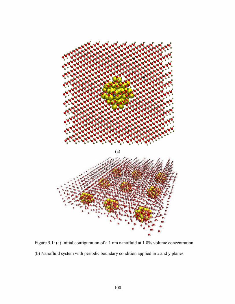
(a)
Figure 5.1: (a) Initial configuration of a 1 nm nanofluid at 1.8% volume concentration,
(b) Nanofluid system with periodic boundary condition applied in x and y planes
100
5.1. Effect of Particle Volume Fraction
The effect of nanoparticle volume fraction on the thermal conductivity of
nanofluids has been studied previously in detail in the literature. Both experimental
[Wang et al 1999, Eastman et al 2001, Patel et al 2003, Murshed et al 2008] as well as
computational [Sarkar & Selvam 2007, Eapen et al 2007, Teng et al 2008] studies have
been conducted to measure the effect of particle volume fraction on transport properties
of nanofluids. Therefore, a comparison study of the thermal conductivity vs. volume
concentration with the previous studies can be done for validation purposes. In the
previous studies, almost a linear increase in the thermal conductivity has been observed
with increasing the volume fraction of the particles. However the slope of this linear
increase in thermal conductivity enhancement with increasing particle volume fraction
was different in different studies [Eastman et al 2001, Xie et al 2003, Eapen et al 2007,
Beck et al 2009]. This linear slope not only depends on the particle volume fraction, but
also depends on the choice of the base fluid and particle type, size of the nanoparticles
and also on the experimental conditions like the system temperature. As mentioned in
chapter 2, thermal conductivity increase of up to 40% was observed by Eastman et al
[2001] for ethylene glycol and copper nanofluid at a mere 0.3% volume concentration
and increase of up to 250% was observed by Choi et al [2001] for carbon nanotube and
oil nanofluid at 1% particle volume fraction. In a molecular dynamic study by Sarkar &
Selvam [2007], thermal conductivity enhancement in model Ar-Cu nanofluid thermal
conductivity enhancement from 14% up to 52% was observed when the particle volume
fraction was increased from 0.5% to 8%. This study showed a steeper increase in thermal
101
conductivity for lower volume fraction of particle and a saturation behavior at higher
volume fractions. Eapen et al [2007] also observed a similar behavior in their molecular
dynamic study of Xe-Pt nanofluid. Once again, it needs to be pointed out that LJ potential
was used for base fluid in these studies.
In this work, a nanofluid system consisting of single nanoparticle surrounded by
water molecules was modeled using the molecular dynamics simulation. Number of
water molecules surrounding the nanoparticle was varied to model nanofluid with
varying volume concentration and to study its effect on the thermal conductivity. A
system containing a 1 nm diameter particle surrounded by 316 to 1696 water molecules
was studied. The volume concentration in various cases considered here varied from 1%
in the lowest case to 5.1% in the highest case. Table 5.1 shows the number of water
molecules and the corresponding volume concentration for 1 nm diameter particle case.
System temperature of 300 ˚K and pressure of 1 atm. was considered in all the cases. Size
of the cubic simulation domain was varied from 2.17 nm for 5.1% volume concentration
to 3.73 nm for 1% volume concentration case to keep the density of water constant at 995
kg/m3.
Thermal conductivity values for the cases considered in Table 5.1 are presented in
Table 5.2 and Figure 5.2. As observed in previous studies the nanofluid thermal
conductivity increases almost linearly from 0.833 W/m.K to 1.346 W/m.K as the particle
volume concentration is increased from 1% to 5.1% for 1 nm particle diameter case.
Thermal conductivity results for 2 nm particle diameter at varying volume concentration
are presented in Table 5.3 and Figure 5.3. As observed in the 1 nm particle case, the data
for 2 nm particle also shows an almost linear increase in thermal conductivity from 0.964
102
W/m.K to 1.588 W/m.K with increase in particle volume concentration from 3.4% to
10.5%.
103

Figure 5.2: Thermal conductivity vs. volume concentration for 1 nm particle
104

Figure 5.3: Thermal conductivity vs. volume concentration for 2 nm particle
105
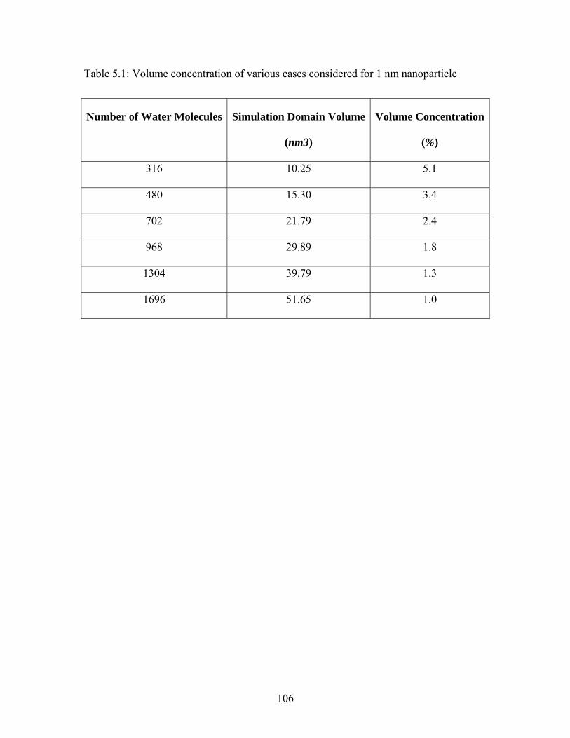
Table 5.1: Volume concentration of various cases considered for 1 nm nanoparticle
Number of Water Molecules Simulation Domain Volume
(nm3)
Volume Concentration
(%)
316 10.25 5.1
480 15.30 3.4
702 21.79 2.4
968 29.89 1.8
1304 39.79 1.3
1696 51.65 1.0
106
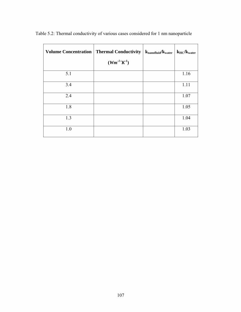
Table 5.2: Thermal conductivity of various cases considered for 1 nm nanoparticle
Volume Concentration Thermal Conductivity
(Wm-1˚K-1)
knanofluid/kwater kHC/kwater
5.1 1.16
3.4 1.11
2.4 1.07
1.8 1.05
1.3 1.04
1.0 1.03
107
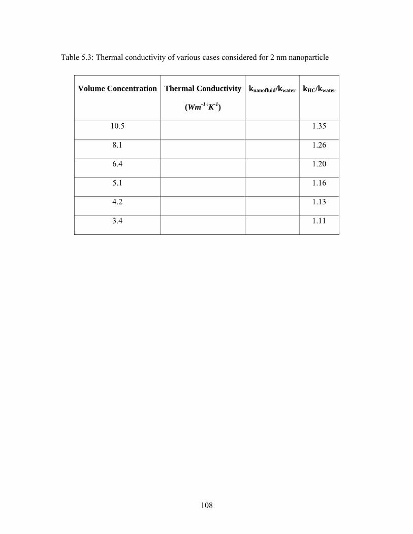
Table 5.3: Thermal conductivity of various cases considered for 2 nm nanoparticle
Volume Concentration Thermal Conductivity
(Wm-1˚K-1)
knanofluid/kwater kHC/kwater
10.5 1.35
8.1 1.26
6.4 1.20
5.1 1.16
4.2 1.13
3.4 1.11
108
The data presented in Table 5.2 and 5.3 qualitatively shows the same trend as
observed by previous molecular dynamics studies of nanofluids [Sarkar & Selvam 2007,
Eapen et al 2007]. Thermal conductivity increase is steeper for lower volume
concentration (up to 2%) and a saturation behavior is observed for higher particle volume
concentration (greater than 2%) where the thermal conductivity increases slowly
compared to that at smaller volume concentrations. Since the nanoparticle considered in
this study is a Lennard-Jones solid, the thermal conductivity data can not be
quantitatively compared with any experimental study, it can only be qualitatively
compared. The thermal conductivity enhancement in this study is higher compared to that
reported by some experimental studies for different nanoparticles at low volume
concentrations and compared to theoretical models as Maxwell model and Hamilton-
Crosser model for various nanoparticles at same volume concentration, but other
molecular dynamic studies [Sarkar & Selvam 2007, Eapen et al 2007, Teng et al 2008,
Wen-Qiang & Qing-Mei 2008] have also observed high thermal conductivity compared
to Maxwell and Hamilton-Crosser models. A discussion on possible reasons for this
behavior is provided later in this chapter.
109
5.2. Effect of Particle Size
As mentioned in chapter 2, the effect of nanoparticle size on the thermal
conductivity of nanofluid is debatable. Researchers have observed both increasing and
decreasing thermal conductivity of nanofluid with increasing the nanoparticle size. To
shed some light on this matter, the effect of particle size is systematically studied in this
work. Nanoparticles of diameter 1 nm, 2 nm, and 3 nm were simulated at the same
volume fraction, system temperature and pressure conditions. Volume fraction of 5.1%
and system temperature and pressure of respectively 300 ˚K and 1 atm. were considered.
The number of water molecules was varied for different nanoparticle diameters to keep
the volume fraction of the nanofluid same. The results of the simulation are presented in
Table 5.4 and Figure 5.4. It is observed that the nanofluid thermal conductivity decreases
with increasing particle diameter. This trend of increasing thermal conductivity with
decreasing particle size has been observed by researchers in the literature [Kang et al
2006, Kim et al 2007, Jang and Choi 2007, Feng et al 2007].
110
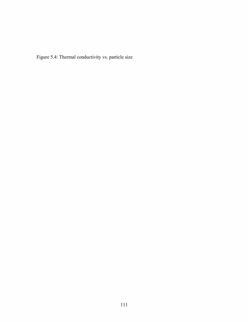
Figure 5.4: Thermal conductivity vs. particle size
111
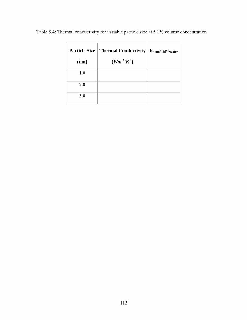
Table 5.4: Thermal conductivity for variable particle size at 5.1% volume concentration
Particle Size
(nm)
Thermal Conductivity
(Wm-1˚K-1)
knanofluid/kwater
1.0
2.0
3.0
112
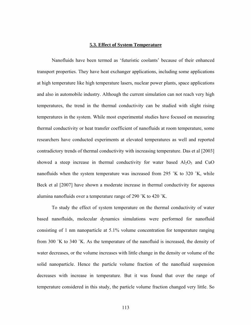
5.3. Effect of System Temperature
Nanofluids have been termed as ‘futuristic coolants’ because of their enhanced
transport properties. They have heat exchanger applications, including some applications
at high temperature like high temperature lasers, nuclear power plants, space applications
and also in automobile industry. Although the current simulation can not reach very high
temperatures, the trend in the thermal conductivity can be studied with slight rising
temperatures in the system. While most experimental studies have focused on measuring
thermal conductivity or heat transfer coefficient of nanofluids at room temperature, some
researchers have conducted experiments at elevated temperatures as well and reported
contradictory trends of thermal conductivity with increasing temperature. Das et al [2003]
showed a steep increase in thermal conductivity for water based Al2O3 and CuO
nanofluids when the system temperature was increased from 295 ˚K to 320 ˚K, while
Beck et al [2007] have shown a moderate increase in thermal conductivity for aqueous
alumina nanofluids over a temperature range of 290 ˚K to 420 ˚K.
To study the effect of system temperature on the thermal conductivity of water
based nanofluids, molecular dynamics simulations were performed for nanofluid
consisting of 1 nm nanoparticle at 5.1% volume concentration for temperature ranging
from 300 ˚K to 340 ˚K. As the temperature of the nanofluid is increased, the density of
water decreases, or the volume increases with little change in the density or volume of the
solid nanoparticle. Hence the particle volume fraction of the nanofluid suspension
decreases with increase in temperature. But it was found that over the range of
temperature considered in this study, the particle volume fraction changed very little. So
113
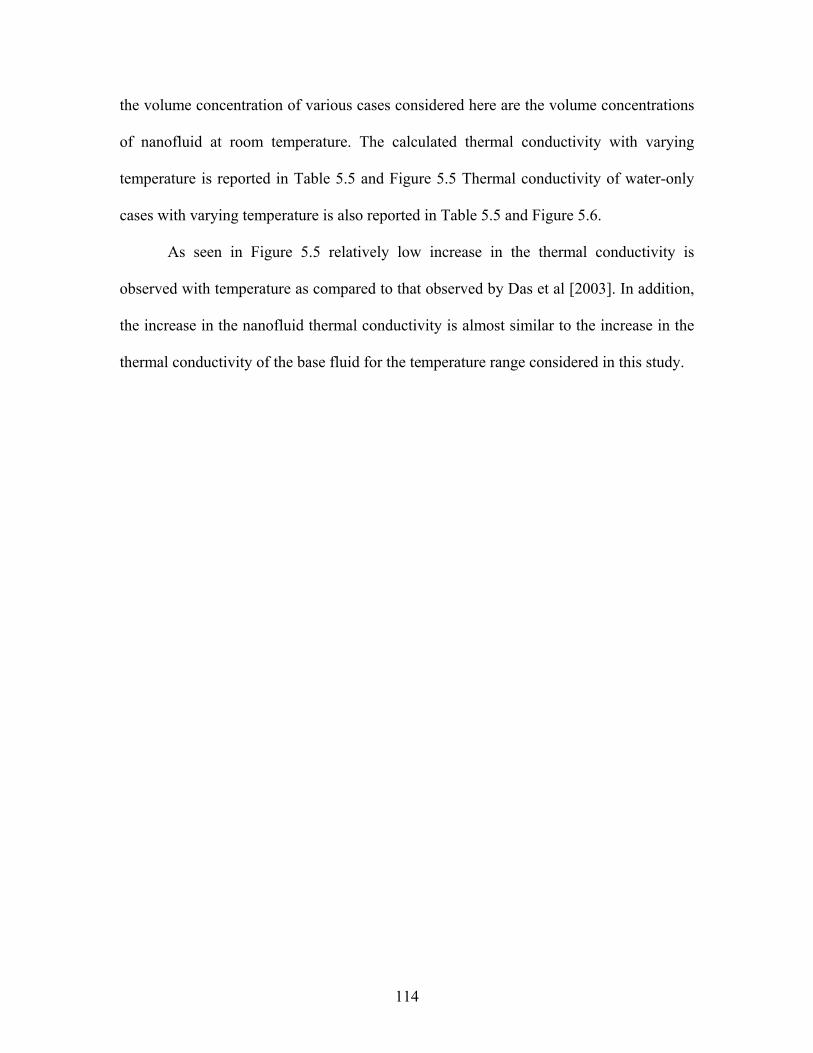
the volume concentration of various cases considered here are the volume concentrations
of nanofluid at room temperature. The calculated thermal conductivity with varying
temperature is reported in Table 5.5 and Figure 5.5 Thermal conductivity of water-only
cases with varying temperature is also reported in Table 5.5 and Figure 5.6.
As seen in Figure 5.5 relatively low increase in the thermal conductivity is
observed with temperature as compared to that observed by Das et al [2003]. In addition,
the increase in the nanofluid thermal conductivity is almost similar to the increase in the
thermal conductivity of the base fluid for the temperature range considered in this study.
114
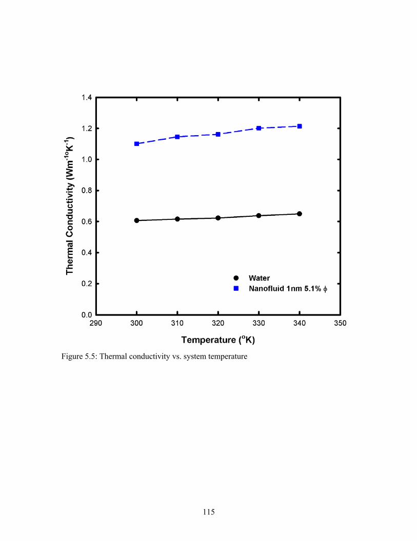
Figure 5.5: Thermal conductivity vs. system temperature
115

Table 5.5: Thermal conductivity at various system temperatures for 1 nm particle case
System Temperature
(˚K)
Nanofluid Thermal
Conductivity (Wm-1˚K-1)
Water Thermal
Conductivity (Wm-1˚K-1)
300 0.606
310 0.615
320 0.623
330 0.638
340 0.649
116
5.4. Effect of Particle Wettability
Most common base fluids considered in nanofluids applications like water and
ethylene glycol are polar in nature and the nanoparticles used in these nanofluids like
oxides (Al2O3, CrO2, SiO2) are chemically reactive. It has been shown that these
nanoparticles (especially Cerium based) may have oxygen vacancies, which can lead to
oxidization in optimal conditions. It has also been reported that the pH of the nanofluid
suspension affects its stability and also transport properties Xie et al [2002]. Various
surfactants are added to stabilize the nanofluid suspension. The presence of surfactants in
these nanofluids also makes the case that the surface chemistry could be playing an
important role in nanofluids. The chemical reactions are not modeled in the current work.
In order to model such interactions with classical molecular dynamics simulation,
quantum molecular dynamics or other sub-atomic computations are required to simulate
such reactions, which is beyond the scope of this work. However, in this work an attempt
is made to study the effects of surface wettability of nanoparticle on the thermal
conductivity of nanofluids. This objective is achieved by varying the strength of the
attractive force between the solid and fluid atoms. The 6-12 Lennard-Jones potential is
considered here as the interaction between the solid and fluid atoms. The r-6 term in the
Lennard-Jones potential accounts for the attractive force between a pair of atoms. A
modified Lennard-Jones potential as proposed by Vladkov & Barrat [2006], is used to
model the solid-fluid interaction for this study. The r-6 term in the Lennard-Jones
potential determines the attraction force between a pair of atoms. A constant ‘c’ is
117
multiplied to the r-6 term in the solid-liquid Lennard-Jones potential, as shown in equation
(5.1), and varying this constant will vary the strength of solid-liquid attraction force.
12 6
4sf sfur rσ σε
⎡ ⎤⎛ ⎞ ⎛ ⎞= −⎢⎜ ⎟ ⎜ ⎟⎝ ⎠ ⎝ ⎠⎢ ⎥⎣ ⎦
c ⎥ (5.1)
The strength of the cross-interaction between solid and liquid atoms can be varied
by changing the parameter ‘c’ in equation 5.1. A low value of parameter ‘c’ would mean
less attraction force between solid-liquid atoms and would model a non-wetting particle,
while a high value of ‘c’ (>1) would mean higher attraction force between a pair of solid-
liquid atoms and would model a highly wetting particle. The value of parameter ‘c’ is
varied from 0.2 to 1.25 in this study to model a range of wetting properties. In their study,
Vladkov & Barrat [2006] varied the parameter ‘c’ to simulate varying Kapitza resistance
at the solid-liquid interface. A higher value of parameter ‘c’ (>1, wetting) translates to
lower Kapitza resistance and a lower value (<1, non-wetting) would model higher
Kapitza resistance at the solid-liquid interface. Results for various cases are reported in
Table 5.6 and Figure 5.6. It is observed that the thermal conductivity increases as the
parameter ‘c’ is increased or in other words, the thermal conductivity is higher for a
wetting particle when compared to a non-wetting particle. These results are important as
they show that if some functionalized particles can be produced and used in these
nanofluids which could improve the wetting nature of these particles, the thermal
conductivity could be enhanced further compared to standard nanoparticles.
118
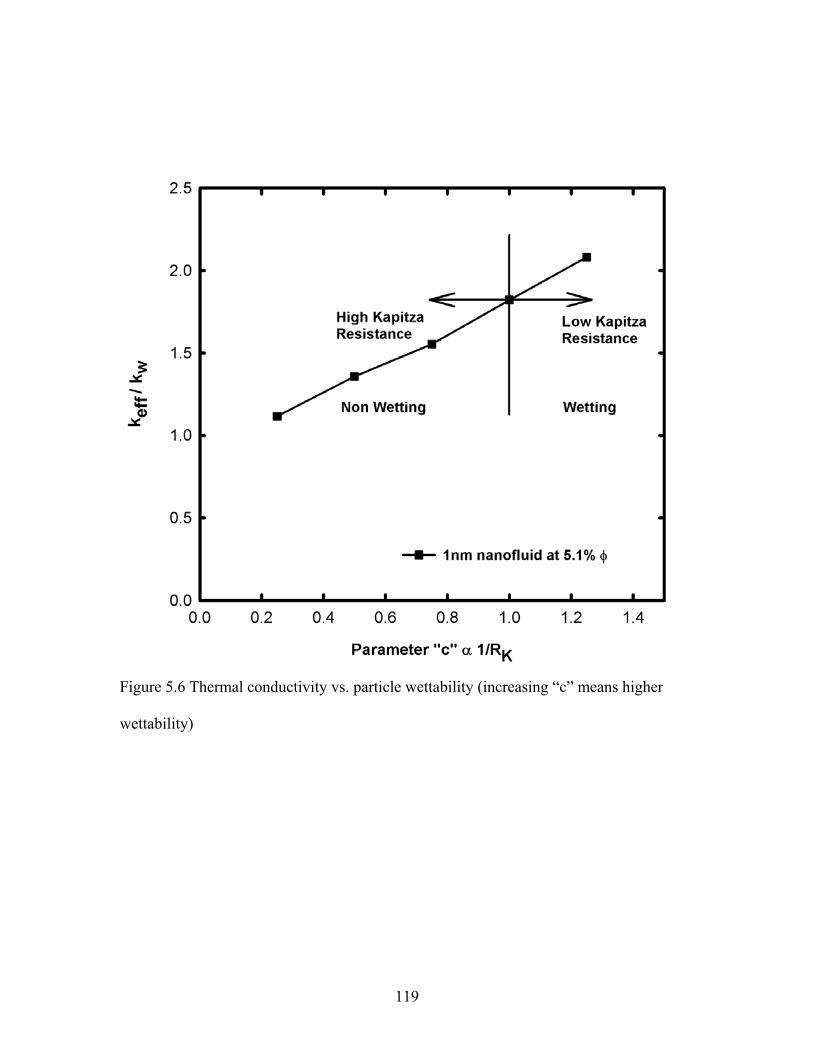
Figure 5.6 Thermal conductivity vs. particle wettability (increasing “c” means higher
wettability)
119
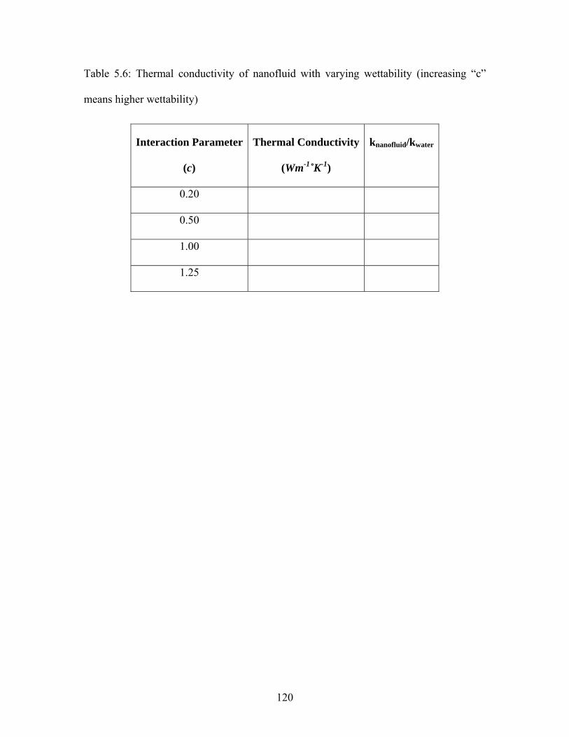
Table 5.6: Thermal conductivity of nanofluid with varying wettability (increasing “c”
means higher wettability)
Interaction Parameter
(c)
Thermal Conductivity
(Wm-1˚K-1)
knanofluid/kwater
0.20
0.50
1.00
1.25
120
5.5. Possible Mechanisms Enhancing Thermal Conductivity in Nanofluids
5.5.1. Hydration Layer Formation at the Solid-Liquid Interface
As discussed in chapter 2, various heat transfer mechanisms have been proposed
in the past to explain the thermal conductivity enhancement in nanofluids. One of the
mechanisms Keblinski et al [2002] proposed was the presence of solid like layer of liquid
molecules or an ordered liquid layer around the solid nanoparticle. This layer of liquid
molecules at the particle-fluid interface is also called ordered liquid layer, second layer or
the hydration layer. Yu and Choi [2003] developed a modified Maxwell model for
effective thermal conductivity of nanofluids. In this model, they assumed that a thin
ordered layer of liquid molecules with higher thermal conductivity compared to the base
fluid is present around the nanoparticle. They concluded that even a very thin liquid layer
would increase the effective volume fraction in the nanofluid and subsequently enhance
the thermal conductivity of nanofluid for particles smaller than 10 nm in diameter. Their
work did not include an MD simulation. Leong et al [2006] also proposed a model and
included the effect of an interfacial liquid layer in their model. They concluded that the
liquid layer at the solid-liquid interface and nanoparticle size are the main parameters
affecting the thermal conductivity of nanofluids. They used a liquid layer of 1 nm
thickness in their model to explain their experimental data.
The interface between a solid and liquid or solid and solid is a study of great
interest since the surface can either provide thermal barrier or thermal enhancement. The
interfacial resistance, also called the Kapitza resistance, arises due to the difference in
121
phonon spectra between the two phases. Nanocrystalline materials with large Kapitza
resistance and grain boundaries less than 40 nm can decrease the thermal conductivity
and provide a thermal barrier [Eastman et al, 2006]. Quite the opposite application of
enhancing thermal conductivity can be found in nanofluids. It is shown that the interfacial
resistance from the collision correlation is not the limiting mechanism in nanofluids
[Eapen et al 2007]. Domingues et al [2005] studied the heat transfer between two
nanoparticles and reported that, as the two nanoparticles are brought closer, the heat
transfer between them is found to be 2 to 3 orders of magnitude more efficient, before
mechanical contact, than when the two nanoparticles are in contact. This means that the
Kapitza resistance between the two nanoparticles before mechanical contact is expected
to be order of magnitude lower as the inter-particle distance becomes smaller. They
concluded that the traditional theories are no longer valid at these length scales. As
shown in this work, when nanoparticles are suspended in water, a hydration layer is
formed around each particle. When there is a strong interaction between the solid and
liquid atoms at the interface, the Kapitza resistance is lower. The hydration layer scatters
the incoming and the outgoing phonons, and influences the interface characteristics, and
increases the nanofluid thermal conductivity. The strong cluster-fluid interaction creates a
dynamic interface around the nanoparticle that facilitates the exchange of energy between
solid and liquid atoms.
The presence of a liquid layer can not be examined easily by an experimental
study. With the advancement of technology, it is possible to look at individual
nanoparticles using Transmission Electron Microscopy (TEM) or Scanning Electron
Microscopy (SEM), but only a small sample of the nanofluid can be put under the
122
scanner in a TEM or SEM. The presence of a liquid layer can only be postulated in
experiments but it can not be confirmed. However in a molecular dynamic simulation all
the details of the atomic trajectory can be captured. The position and velocities of liquid
and solid atoms are recorded at every step. To check the presence of the liquid layer
around the solid nanoparticle, the density distribution of liquid atoms around the
nanoparticle can be examined using the trajectory data. Using the recorded positions of
liquid and solid atoms during the simulation, the number of liquid molecules can be
counted in a specified space around the nanoparticle in the simulation domain. So the
simulation domain is divided in to multiple concentric spherical shells around the
nanoparticle, as shown in Figure 5.7 [Teng et al, 2008], and the number density of liquid
molecules is calculated in these spherical shells.
The number density is defined as number of atoms per unit volume.
nnVΔ
=Δ
(5.2)
Here, is the number of atoms in a specified volumenΔ VΔ . In this case the
volume is the volume of each concentric spherical shell of thickness as shown in
Figure 5.7. The number of liquid molecules in each of these shells is counted at different
time intervals to calculate the number density. Figure 5.8 shows the distribution of
relative number density of liquid molecules around the nanoparticle at various times.
Relative number density
VΔ trΔ
o
nn
is defined as the number density of liquid molecules in the
nanofluid at some time (t) during the simulation (n), divided by the number density of
liquid (no) at time zero. It is observed from Figure 5.8 that the density of water is high
near the surface of the nanoparticle and it decreases as the distance from the nanoparticle
123
surface increases. This observation confirms the presence of the interfacial liquid layer as
postulated by researchers in the literature. It is also observed from Figure 5.8 that the
thickness of the ordered liquid layer is about 0.5 nm, which is consistent with observation
made by Li et al [2008]. They conducted an MD study and used the LJ potential to
simulate interactions between all atom pairs of a model nanofluid system. They used the
Lennard-Jones parameters of argon for liquid and copper for solid atoms. They did not
report any quantitative results for thermal conductivity enhancement but showed the
presence of a layer of liquid molecules at the solid-liquid interface of the order of 0.5
nanometer.
By tracking the movement of liquid atoms around the nanoparticle, the presence
of a liquid layer at the solid-liquid interface is confirmed. This liquid layer is formed
because of the stronger interatomic force between the solid-liquid atoms as compared to
the interatomic force between the liquid atoms. This finding is important in
understanding the heat transfer mechanisms in nanofluids. This finding confirms the
contribution of ordered liquid layer to the enhancement of thermal conductivity as
proposed by Jang and Choi [2004], “thermal interaction of nanoparticle with base fluid”,
and by Ren et al [2005], “enhancement by nanolayer” and by Keblinski et al [2002],
“liquid layering at liquid-particle interface”.
124
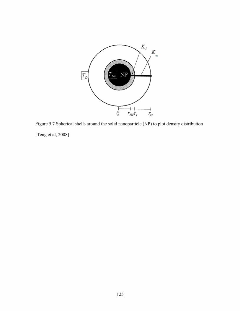
Figure 5.7 Spherical shells around the solid nanoparticle (NP) to plot density distribution
[Teng et al, 2008]
125
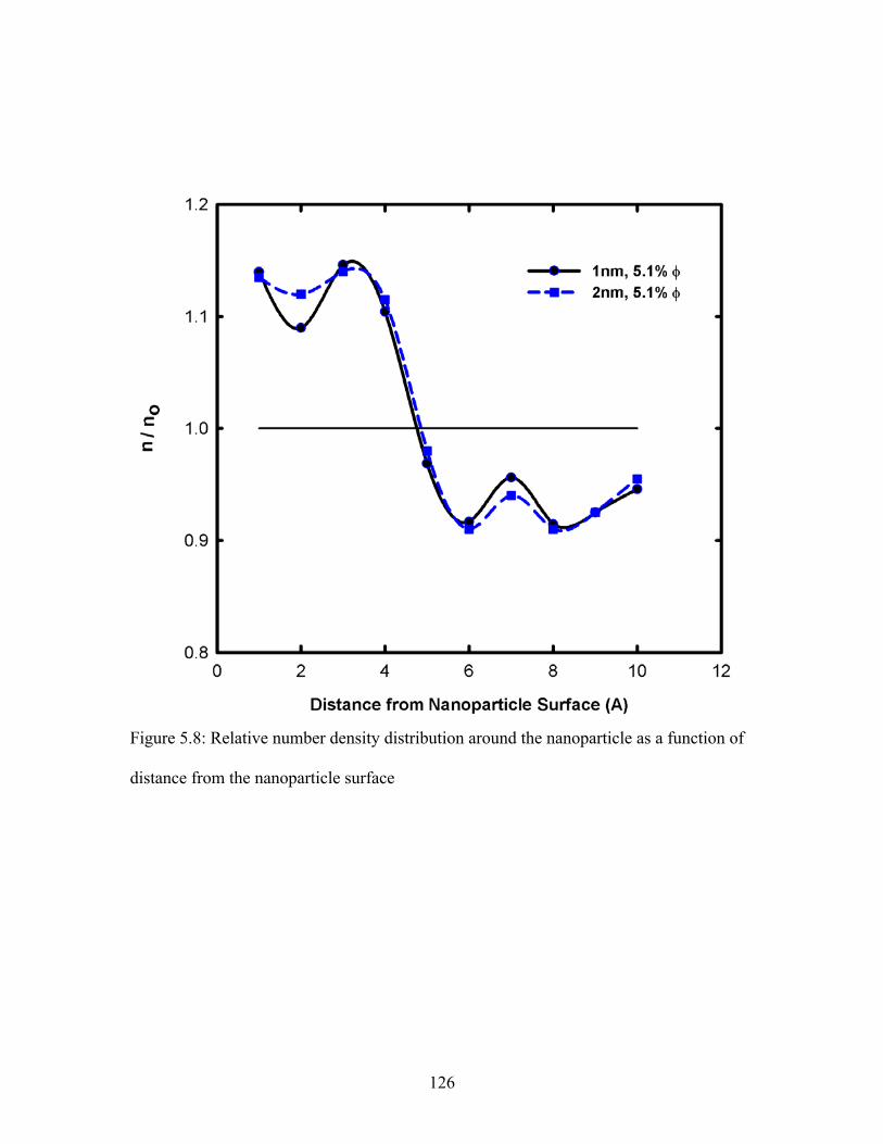
Figure 5.8: Relative number density distribution around the nanoparticle as a function of
distance from the nanoparticle surface
126
5.5.2. Mean Square Displacement (MSD)
In this section another mechanism causing the thermal conductivity enhancement
in nanofluids is discussed. As stated in previous section movement of all the liquid and
solid atoms in the simulation domain can be easily tracked in molecular dynamics
simulation. The movement and interaction of these atoms and molecules at atomic scale
is the cause of all macro-scale properties of any material, including the enhanced thermal
conductivity of nanofluids. By using the atomic position data at various time steps the
mean square displacement (MSD) can be calculated for the liquid and solid molecules.
Comparison of the MSD of liquid molecules in the base fluid and in the nanofluid at
varying volume concentration can give an insight into the thermal transport mechanism in
nanofluids. The MSD is a measure of the distance travelled by an atom or a molecule. It
is defined as:
( ) ( ) ( ) ( )2
2 0i i iMSD t r t r t r→ → →⎛= Δ = −⎜
⎝ ⎠⎞⎟
⎞⎟
(5.3)
Here, is the position of atom i at time t, and is the vector
distance traveled by an atom i, over a time interval t. The angular brackets
( )ir t→
( ) ( )0i ir t r→ →⎛ −⎜⎝ ⎠
mean
average over all atoms. The square of the displacement undergone by all N atoms is
averaged to give the mean value. So the above equation gives the mean square
displacement of all the molecules in the fluid over a time period t. The angular bracket is
also known as ‘ensemble average’. To get the MSD of liquid molecules in the nanofluid
only the displacement of liquid molecules is considered in the above equation.
127
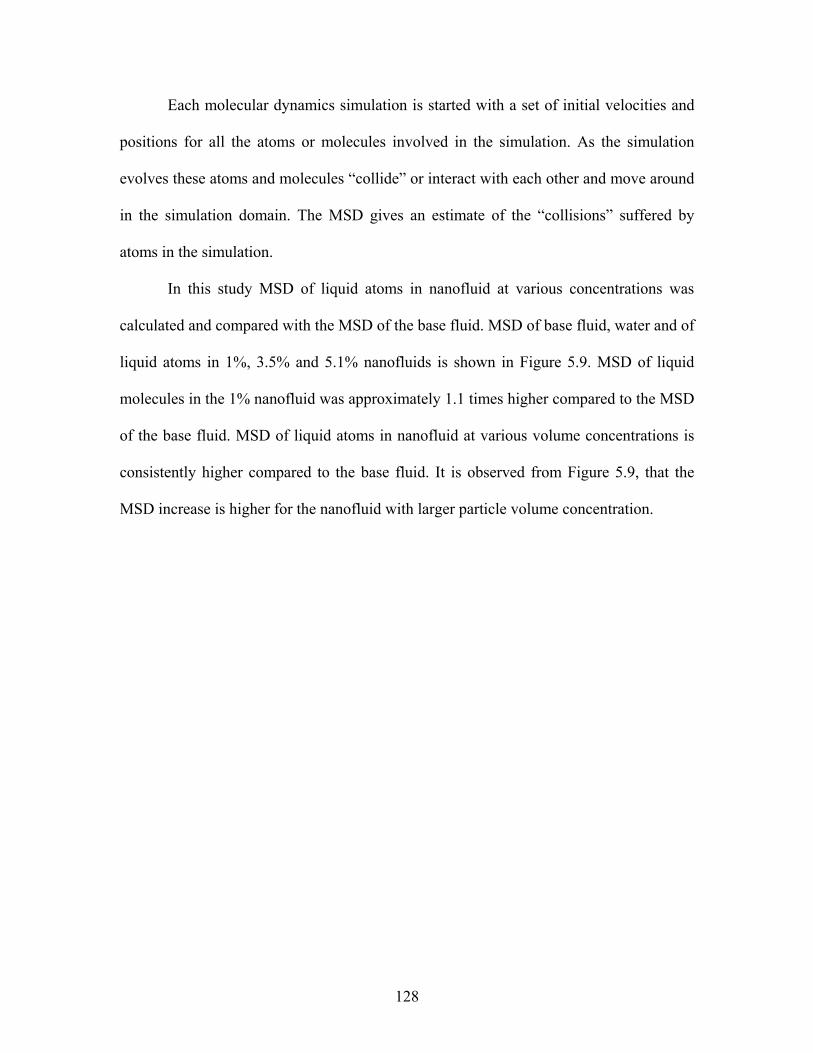
Each molecular dynamics simulation is started with a set of initial velocities and
positions for all the atoms or molecules involved in the simulation. As the simulation
evolves these atoms and molecules “collide” or interact with each other and move around
in the simulation domain. The MSD gives an estimate of the “collisions” suffered by
atoms in the simulation.
In this study MSD of liquid atoms in nanofluid at various concentrations was
calculated and compared with the MSD of the base fluid. MSD of base fluid, water and of
liquid atoms in 1%, 3.5% and 5.1% nanofluids is shown in Figure 5.9. MSD of liquid
molecules in the 1% nanofluid was approximately 1.1 times higher compared to the MSD
of the base fluid. MSD of liquid atoms in nanofluid at various volume concentrations is
consistently higher compared to the base fluid. It is observed from Figure 5.9, that the
MSD increase is higher for the nanofluid with larger particle volume concentration.
128
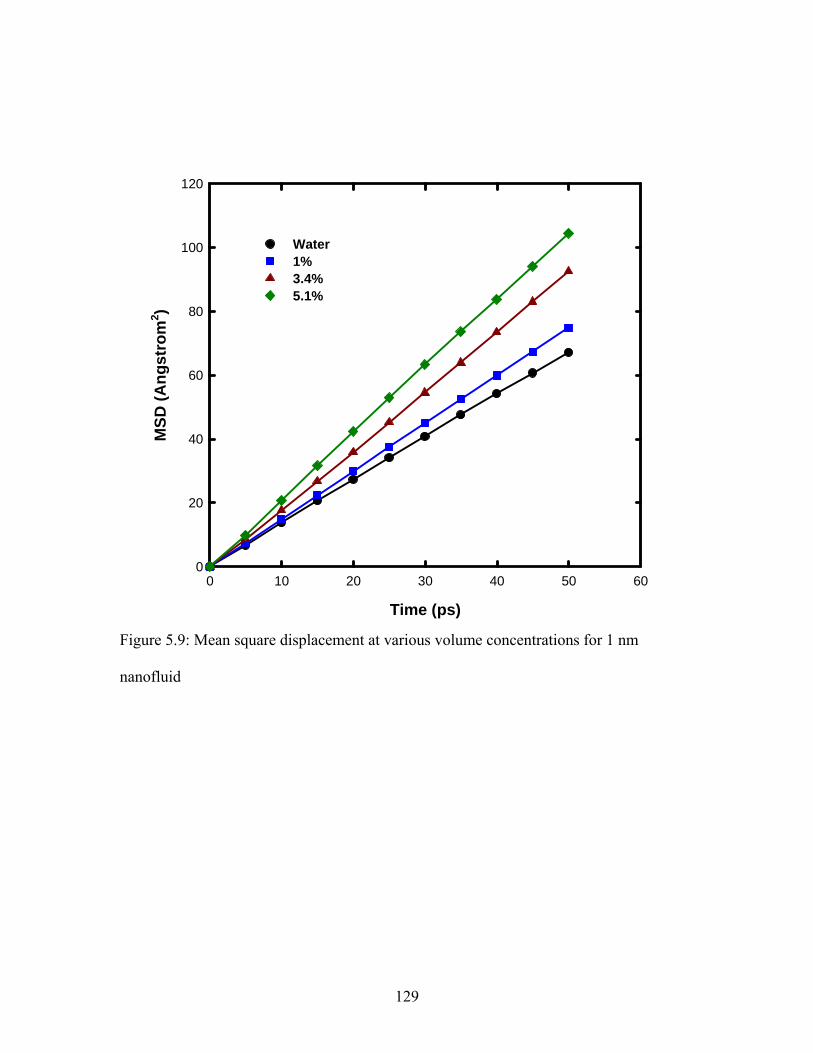
Time (ps)
0 10 20 30 40 50 60
MSD
(Ang
stro
m2 )
0
20
40
60
80
100
120
Water1%3.4%5.1%
Figure 5.9: Mean square displacement at various volume concentrations for 1 nm
nanofluid
129
In dilute gases, the intermolecular forces play no role and the mean free path is
larger, so the molecules spend most of their time in free flight between brief collisions
when their direction and speed changes. Thus, random molecular motions are responsible
for the gaseous transport process. In liquids, however, mean free path is smaller and the
molecules are closely packed and are in a collision state. These frequent collisions
between liquid molecules are responsible for thermal transport in liquids. The comparison
of MSD for various nanofluids as observed in Figure 5.9, shows that there is significant
increase in the movement and hence the displacement of the liquid molecules due to the
presence of solid nanoparticles. This enhanced movement will eventually mean that the
liquid molecules undergo more frequent “collisions” and hence transport more energy.
This is accentuated by the fact that there are additional liquid molecules close to the
nanoparticle in the form of hydration layer. Since these liquid molecules are more closely
packed than other liquid molecules away from the particle, the attraction or cohesive
potential between the liquid molecules are dominant. The increased movement of liquid
molecules in the hydration layer close to the nanoparticle, as well as away from the
nanoparticle is due to the interatomic interaction between the solid and liquid atoms,
which is much stronger compared to the interatomic potential between the liquid atoms.
This enhanced motion of water molecules combined with the hydration layer around the
nanoparticle can significantly enhance the thermal conductivity of nanofluids.
130
5.5.3. Diffusion Coefficient
Various transport coefficients can be calculated using the equilibrium correlations
on the position, velocity and force data generated from molecular dynamics simulations.
The Einstein’s relation [Rapaport, 2004] can be used to calculate the diffusion coefficient
(D) from the MSD data. The self-diffusion coefficient is given as:
( )2
23limi
t
r tD
t
→
→∞
Δ= (5.4)
The limiting slope of MSD for large time gives the self-diffusion coefficient from
above expression. Using equation 5.4 the diffusion coefficient of the base fluid, and
liquid molecules in nanofluid is calculated for various volume concentrations. The
diffusion coefficient of water was found to be 0.224 2Ao
ps . The experimental value of
the diffusion coefficient of water is 0.24 2Ao
ps . So our molecular dynamic simulation
reasonably predicts the diffusion coefficient of pure water. The diffusion coefficient of
1%, 3.4% and 5.1% volume concentration nanofluid cases were also calculated and
compared with the diffusion coefficient of pure water. The diffusion coefficient results
for various cases considered are presented in Table 5.7. Figure 5.10 shows the ratio of the
diffusion coefficient of liquid in nanofluid (Deff) to the diffusion coefficient of pure water
(D) for various volume concentrations of nanofluids. It is observed that diffusion
coefficient of nanofluid increases almost linearly with increasing particle concentration.
This finding is consistent with the results reported by Sarkar and Selvam [2007] for a
model Ar-Cu nanofluid system. Comparing Figure 5.10 diffusion coefficient with thermal
131
conductivity, it is seen that both diffusion coefficient and thermal conductivity increase
almost linearly with increasing volume fraction of nanofluid. This shows a strong
correlation between the thermal conductivity and diffusion coefficient enhancement. The
diffusion coefficient in nanofluid is calculated from the MSD, which shows that the
increase in diffusion coefficient with increasing volume concentration is because of the
enhanced motion of liquid molecules due to the presence of solid nanoparticle. So this
enhanced motion of liquid molecules in the hydration layer is responsible for the
enhanced thermal conductivity of nanofluids.
132
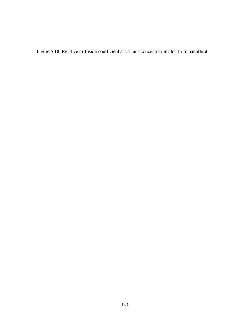
Figure 5.10: Relative diffusion coefficient at various concentrations for 1 nm nanofluid
133
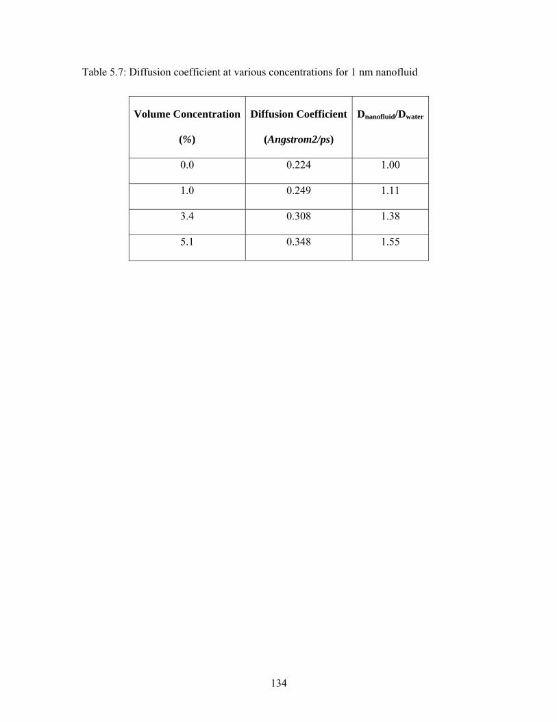
Table 5.7: Diffusion coefficient at various concentrations for 1 nm nanofluid
Volume Concentration
(%)
Diffusion Coefficient
(Angstrom2/ps)
Dnanofluid/Dwater
0.0 0.224 1.00
1.0 0.249 1.11
3.4 0.308 1.38
5.1 0.348 1.55
134
5.5.4. Heat Current Autocorrelation Function (HCAF) Decomposition
The thermal conductivity of nanofluids in this work is calculated using the Green-
Kubo correlation of the heat current. In the linear response region, various transport
properties e.g. thermal conductivity, viscosity and diffusion coefficient etc can be
calculated using the time correlation. The thermal conductivity is calculated using the
time integral of the HCAF as given by equation 3.21. is the instantaneous heat flux
vector as given by equation 3.24. Eapen et al [2007] while studying the dominating heat
conduction mechanisms in nanofluids decomposed the heat flux vector in its three
constituents, namely (1) kinetic, (2) potential, and (3) collision. The total heat flux can be
written as sum of 3 terms as given below:
q→
K P Cq q q q→ → → →
= + + (5.5)
This decomposition can also be looked at as sum of convective and inter-atomic
terms as proposed by Teng et al [2008]. First two terms in equation 5.5 denote the energy
transported due to the convective effect and the third term is the energy transport due to
the inter-atomic collisions of atoms and molecules in the system. Thermal conductivity
for various volume concentrations of 1 nm particle were calculated using this
decomposed form of the heat flux vector to compare the contributions to the thermal
conductivity of nanofluid from kinetic, potential and collisions mechanisms.
Figure 5.11 shows the variation of overall nanofluid thermal conductivity and the
contribution to overall conductivity from each of these modes. It is observed that most of
the thermal conductivity comes from the collision mode in pure water. The collision
135
mode which arises from the inter-atomic interactions between the atoms and molecules is
also dominant in the thermal conductivity of the nanofluid. This observation is consistent
with the observations made by Eapen et al [2007] in their molecular dynamics study of
the Xe-Pt model nanofluid. Another important observation from Figure 5.11 is that the
increase in thermal conductivity with increasing volume fraction of the nanoparticle
mainly comes from the same collision mode. This observation is in contrast to what was
observed by Eapen et al [2007] that the increase in thermal conductivity with increasing
volume fraction comes from the potential mode as opposed to the collision mode. Their
work did not include any hydration layer around the particle. Their MD simulation
consisted of nanoparticles that had 10 atoms and were less than 1 nm in size. In the
decomposition analysis of the heat current, they reported that the potential energy
increase due to the solid-liquid interaction caused the nanofluid thermal conductivity
enhancement. They said the solid-liquid interaction caused the exchange of energy
between the solid and liquid atoms, however it was not clear how this exchange was
taking place. Sarkar & Selvam [2007] reported an increase in MSD and diffusion
coefficient due to the presence of the nanoparticle. But they too did not consider the
hydration layer formation.
136
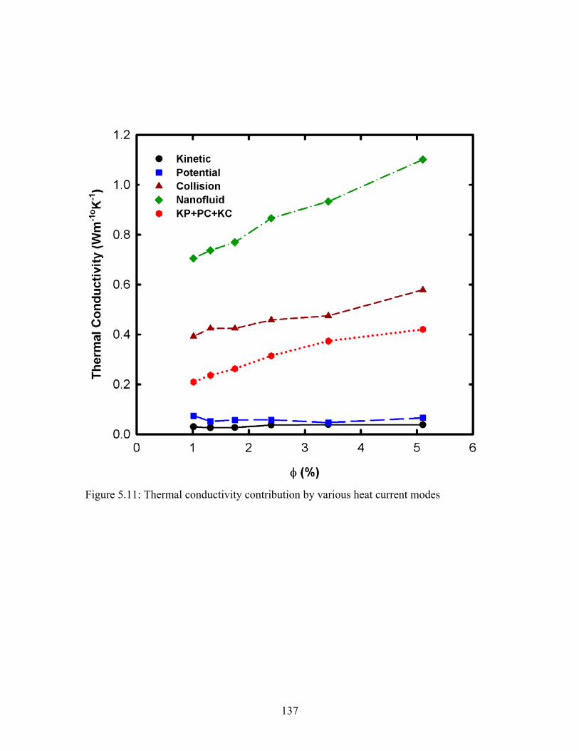
Figure 5.11: Thermal conductivity contribution by various heat current modes
137
5.5.5. Strong Particle-Fluid Interaction
In the previous sections, it was shown that the presence of nanoparticles in water
affects the motion of the water molecules and a hydration layer of water molecules is
formed around the nanoparticle. These two phenomena occur due to the strong particle-
fluid interaction present in the nanofluid. The effect of the strength of this particle-fluid
interaction on the thermal conductivity of nanofluid was shown in section 5.4. The
strength of solid-liquid interaction was modified by using an interaction coefficient “c” in
the modified Lennard-Jones potential. It was observed that the thermal conductivity of
the nanofluid increases with increasing the value of the interaction coefficient “c”, which
translates to increasing the attractive force between the solid-liquid atoms. It has been
shown by Vladkov and Barrat [2008] that a low value of this interaction coefficient
means a higher interfacial resistance, also called Kapitza resistance. So our results show
that a lower value of interfacial resistance would lead to higher thermal conductivity in
nanofluids.
These results show that if functionalized nanoparticles can be produced that are
hydrophilic in nature, this could further enhance the thermal conductivity of nanofluids
compared to normal nanoparticles. This fact also brings to light the importance of
stabilizers used in nanofluids. Various surfactants are used to stabilize these nanofluids
and other methods like modifying the pH of the suspension are also used to improve the
stability of the nanofluids. The surfactants are long chain like molecules that attach
themselves to the surface of the nanoparticle and deter them from agglomerating with
each other and settling down with time. So these surfactants molecules cause the
138
nanoparticle to repel each other. If a surfactant used to stabilize the nanoparticles in a
nanofluid causes the nanoparticles to have weaker interaction with the fluid atoms, it can
lead to a lower thermal conductivity of the nanofluid. This means that a water-alumina
nanofluid of same volume concentration and same original nanoparticle size can have
different transport properties if the surfactant used in these suspensions affect the
particle-fluid interaction in different ways. Some of the surfactants used by companies
that manufacture nanofluids are proprietary and details of these surfactants are not
disclosed to the buyer. So what effect these unknown surfactants might have on the
transport properties of nanofluids is debatable.
139
CHAPTER SIX: SUMMARY & FUTURE WORK
In the development of energy efficient heat transfer fluids, required for the
cooling applications in many industries, the low thermal conductivity of conventional
fluids is a primary limitation. Nanofluids consisting of nanometer size solid particles
dispersed in base fluids, have demonstrated great potential in improving the heat transfer
characteristics of liquids. Even though research has been done in the area of nanofluids in
the past decade, it is still an immature research field. The limitation hindering the use of
nanofluids in mainstream cooling applications is the lack of understanding of thermal
enhancement of nanofluids in single-phase stationary or flowing situations or in two-
phase boiling condition. Before these nanofluids could be used in engineering
applications, it is of paramount importance to reliably measure and/or predict the thermal
conductivity and viscosity of various nanofluid systems as a function of particle volume
fraction, size and system temperature. Significant research work has been conducted in
measuring thermal conductivity of nanofluids, with inconclusive results. Although the
potential for the use of nanofluids in heat transfer applications is promising, a major
stumbling block hindering the development of this field is that, a detailed atomic-level
understanding of the mechanisms responsible for the thermal transport enhancement
remains elusive.
A systematic study using computer simulation is required to determine the cause
of thermal conductivity enhancement and explore these mechanisms at nanoscale. Due to
the length scale involved in nanofluids conventional macroscale computational
techniques like CFD and FED can not be used here. We believe that modeling of
140
nanofluids at atomic scale using molecular dynamics (MD) simulation can provide
valuable insights in understanding the origins of enhancement of various transport
properties in nanofluids. With molecular dynamic simulation we can examine the
interplay between solid and liquid atoms occurring at molecular level, which determines
the macroscale transport properties.
In this work a molecular dynamic simulation tool is developed to study possible
mechanisms causing the thermal conductivity enhancement in water based nanofluids.
Previous studies involving MD simulation of nanofluids have considered simplistic
Lennard-Jones (LJ) potential to model the interactions between both solid and liquid
atoms. In this work, liquid water is modeled as a flexible bipolar molecule using the
Flexible 3 Center (F3C) model. Since the complex surface chemical reactions between
the solid nanoparticle and fluid atoms have not yet been identified by experiments and
expensive quantum-chemistry based simulations are required to identify them, a simple
two body LJ potential is used to model the solid nanoparticle. In addition, each atom in
the nanoparticle is connected to its first neighbors by finite extensible nonlinear elastic
(FENE) bonding potential. The thermal conductivity is calculated by combining the
linear response theory with molecular dynamic simulation (Green-Kubo formulation).
The molecular dynamic tool is validated for liquid argon and water only systems and an
excellent match is found between thermal conductivity calculated from this tool and
between the experimental measurements. To date this work is the first to use a realistic
potential to model the liquid (water) molecules using molecular dynamic simulation.
A systematic investigation involving particle volume fraction, size, wettability
and system temperature is undertaken using molecular dynamic simulation and the effect
141
of these parameters on the thermal conductivity of nanofluids is studied. The various
atomic interactions show that there exist two regimes of thermal conductivity
enhancement with particle volume fraction, which has also been previously observed in
the literature. It is also found that increasing particle size decreases thermal conductivity
enhancement, which is consistent with the previous studies. In contrast to previous
studies, it is observed that increasing system temperature does not enhance the system
thermal conductivity significantly. The temperature dependence in the nanofluid arises
mostly from the temperature dependence of the base fluid. It is also seen that increasing
the wettability of nanoparticle causes an increase in thermal conductivity enhancement.
These findings show that the surface interactions between solid-liquid atoms are very
important and functional nanoparticles which are hydrophilic in nature would show
higher enhancement in thermal conductivity compared to regular nanoparticles.
By tracking the motion of solid and liquid molecules we show that a hydration
layer is formed at the particle-fluid interface. It is also observed that the motion of liquid
molecules is enhanced due to the presence of solid particles, which was captured by
comparing the mean square displacement (MSD) of liquid molecules in nanofluid to that
of the MSD of base fluid. The microscopic heat flux vector is decomposed into three
modes, namely kinetic, potential and collision. It is observed that the significant
enhancement comes from the collision mode, which arises from the enhanced motion of
the liquid molecules. The dense hydration layer at the solid-liquid interface and the
enhanced motion of the liquid molecules also create a possibility of cooperative or
coherent exchange of thermal transport between the solid and liquid molecules, which
enhances the nanofluid thermal conductivity.
142
1.1 Future Work
This thesis advances the atomic level understanding of mechanisms causing
thermal conductivity enhancement in nanofluids using molecular dynamics simulation. A
realistic flexible bipolar water molecule was used to model the base fluid in this work.
However, in complex chemical reactions between the nanoparticle and liquid molecules
in the presence of chemical dispersant was not considered in this work. Experimental and
quantum molecular dynamic studies are needed to first identify these chemical reactions
and to develop appropriate potentials to model them using molecular dynamic simulation.
In this work a Lennard-Jones potential with FENE bonding potential was used to model
the solid nanoparticle, which would closely mimic the behavior of a non-metallic
nanoparticle. A general water based nanofluid system was studied in this work. To
predict the thermal conductivity enhancement of a specific nanofluid system, more
sophisticated potentials could be used, e.g. to model metallic nanoparticles, embedded
atom method (EAM) potential which can also take care of the metallic bonding should be
used. To get most quantitatively accurate results for a particular metal, EAM potential
with appropriate parameters for that material should be used.
In addition, various experimental studies have cited nanoparticle agglomeration as
an important mechanism causing the thermal conductivity enhancement in nanofluids. In
future molecular dynamic studies, the effect of nanoparticle agglomeration on thermal
conductivity enhancement should be studied. But, in order to model the nanoparticle
agglomeration, a reliable particle-particle interaction potential needs to be established.
Experimental work involving the surface chemistry of nanoparticles is required to
understand the particle-particle interaction in nanofluids.
143
Although several research articles have appeared on the measurements of various
properties of nanofluids in a static environment, not much has been reported on the
measurement of heat transfer coefficient of nanofluids in a flowing situation. In any
engineering application, the nanofluids would be used in a forced convection situation, so
it is important to measure the transport properties of nanofluids in those conditions. It has
not been reported how various properties of nanofluids change with time. With time,
some of the nanoparticles could agglomerate or settle down in the channel and this could
affect the effectiveness of nanofluids. The effect of time and forced flow will remain an
active area for future research in nanofluids.
144
LIST OF REFERENCES
Ahuja A.S., J. Appl. Phys. 46(8), 3408 (1975)
Alder B. J. and Wainwright T. E., J. Chem. Phys. 31 (2), 459 (1959)
Allen M.P. and Tildesley D.J., Computer Simulation of Liquids, Oxford, Oxford Science
Publications (1987)
Assael, M.J., Metaxa I.N., Kakosimos K., and Constantinou D., Intl. J. Thermophysics,
27(4), 999 (2006)
Beck M.P., Sun T. and Teja A., Fluid Phase Equilibria 260(2), 275 (2007)
Beck M.P., Yuan Y., Warrier P. and Teja A., J. Nanopart. Res. 11(5), 1129 (2009)
Berber S., Kwon Y. K.and Tomanek D., Phys. Rev. Lett. 84(20), 4613 (2000)
Berendsen H.J.C., Postma J.P.M, van Gunsteren W.F., and Hermans J., Intermolecular
Forces, Pullman B., Ed., Reidel, Dordrecht, 331, (1981)
Berendsen H.J.C., Grigera J.R. and Straatsma T.P., J. Phy. Chem. 91, 6269 (1987)
Bertolini D. and Tani A., Phys. Rev. E. 56, 4135 (1997)
Bhattacharya P., Saha S.K., Yadav A., Phelan P.E. and Prasher R.S., J. Appl. Phys. 95,
6492 (2004).
Che J., Cagin T., Deng W., and Goddard W.A., J. Chem. Phys. 113(16) 6888 (2000)
Choi S.U.S., Development and Applications of Non-Newtonian Flows, ASME, FED-Vol.
231/MD-Vol. 66, 99-103 (1995)
Choi S.U.S., Zhang Z.G., Yu W., Lockwood F.E., and Grulke E.A., Appl. Phys. Lett.
79(14), 2252 (2001).
145
Choi S.U.S., Zhang Z.G. and Keblinski P., Nanofluids, Encyclopedia of Nanoscience and
Nanotechnology, 6, 757 (2004)
Chon, C.H., K.D. Kihm, S.P. Lee, and S.U.S. Choi, Appl. Phys. Lett. 87(15), 153107
(2005)
Clarke J.H.R., Smith W., and Woodcock L. V., J. Chem. Phys. 84, 2290 (1984).
Das S.K., Putra N., Thiesen P., and Roetzel W., J. Heat Transfer 125, 567 (2003).
Demontis P., Spann S. and Suffritti G.B., J. Chem. Phys. 114, 7980 (2001)
Eapen J., Li J. and Yip S., Phys. Rev. Lett. 98(2), 028302 (2007)
Eastman J.A., Choi S.U.S., Li S., Soyez G., Thompson L.J., and Di Melfi R.J., Mater.
Sci. Forum 312-314, 629 (1999)
Eastman J.A., Choi S.U.S., Li S., Yu W., and Thompson L.J., Appl. Phys. Lett. 78, 718
(2001)
Eastman J.A., Philpot S.R., Choi S.U.S. and Keblinski P, Annu. Rev. Mater. Res. 34, 219
(2004)
Eastman J.A., Yang H.S., Thompson L.J. and Bai G.R.
http://chemistry.anl.gov/MSDReview/Complex_Oxides/KapitzaYSZ.pdf (2006)
Evans W., Fish J. and Keblinski P., Appl. Phys. Lett. 88, 093116 (2006)
Evjen H.M., Phys. Rev. 39, 675 (1932)
Florain M., J. Chem. Phys. 106, 6082 (1997)
Gupta A., and Kumar R., Appl. Phys. Lett. 91, 223102 (2007)
Haile J. M., Molecular Dynamics Simulation, New York, John Wiley & Sons (1997)
Hamilton R.L. and Crosser O.K., I&EC Fundamentals 1(3), 187 (1962)
146
Hoheisel C., Theoretical Treatment of Liquids and Mixtures, Elsevier Publishing
Company (1987)
Hong T., Yang H. and Choi C.J., J. Appl. Phys. 97(6), 064311 (2005)
Hwang, Y.J., Ahn Y.C., Shin H.S., Lee C.G., Kim G.T., Park H.S., and Lee J.K., Curr.
Appl. Phys. 6(6), 1068 (2006)
Hwang, Y., Lee J.K., Lee C.H., Jung Y.M., Cheong S.I., Lee C.G., Ku B.C., and Jang
S.P., Thermochimica Acta, 455(1), 70 (2007)
Jana, S., Salehi-Khojin A., and Zhong W.H., Thermochimica Acta, 462(1), 45 (2007)
Jang S.P. and Choi S.U.S., Appl. Phys. Lett. 84, 4316 (2004)
Kaburaki H., Li J., and Yip S., Mater. Res. Soc. Symp. Proc. 538, 503 (1999)
Kang, H.U., Kim S.H., and Oh J.M., Expt. Heat Transfer, 19(3), 181 (2006)
Kapitza P.L., J. Phys. USSR 4:181, Zh. Eksp. Teor. Fiz. 11, 1 (1941)
Keblinski P., Philpot S.R., Choi S.U.S. and Eastman J.A., Int. J. Heat & Mass Transfer
45, 855 (2002)
Keblinski P., Prasher R. and Eapen J., J. Nanopart. Res., 10(7), 1089 (2008)
Kim P., Shi L., Majumdar A. and McEuen P.L., Phys. Rev. Lett. 87, 215502 (2001)
Kim, S.H., Choi S.R., and Kim D., J. Heat Transfer 129(3), 298 (2007)
Kumar, D.H., Patel H.E., Kumar V.R.R., Sundararajan T., Pradeep T., and Das S.K.,
Phys. Rev. Lett. 93(14), 144301 (2004)
Lee S., Choi S.U.S, Li S. and. Eastman J.A, Trans. ASME J. Heat Transfer 121, 280,
(1999)
Lennard-Jones J.E., Proceedings of the Royal Society (London) 106A, 441 (1924)
Leong K.C, Yang C. and Murshed S.M.S., J. Nanopart. Res. 8(2), 245 (2006)
147
Levitt M., Hirshberg M., Sharon R., Laidig K.E. and Daggett V., J. Phys. Chem. B 101
(25), 5051 (1997)
Li, C.H. and G.P. Peterson, J. Appl. Phys. 101(4), 044312 (2007)
Li L., Zhang Y., Ma H. and Yang M., Phys. Lett. A 372, 4541 (2008)
Liu K.V., Choi S.U.S. and Kasza K.E., Argonne National Laboratory Report, ANL-88-
15, (1988)
Liu, M.S., Lin M.C.C., Tsai C.Y., and Wang C.C., Intl. J. of Heat Mass Transfer, 49(17),
3028 (2006)
Lu W. and Fan Q., Engineering Analysis with Boundary Elements, 32(4), 288 (2008)
Masuda H., Ebata A., Teramae K., and Hishinuma N., Netsu Bussei (Japan) 4, 227
(1993)
Maxwell J.C., A treatise on electricity and magnetism, II ed., Vol. 1, Clarendon press,
Oxford, U.K., 435, (1881)
McGaughey A.J.H. and Kaviany M., Int. J. Heat and Mass Transfer 47, 1799 (2004)
McQuarrie, D.A., Statistical Mechanics, 2nd ed., University Science Books, California,
(2000)
Murshed S.M.S., Leong K.C. and Yang C., Int. J. Therm. Sci. 44(4), 367, (2005)
Murshed S.M.S., Leong K.C. and Yang C., J. Phys. D: Appl. Phys. 39(24), 5316, (2006)
Murshed S.M.S., Leong K.C. and Yang C., Int. J. Therm. Sci. 47(5), 560, (2008)
Müller-Plathe, F. J. Chem. Phys. 106, 6082 (1997)
Patel H.E., Das S.K., Sundarajan T., Nair A.S., George B. and Pradeep T., Appl. Phys.
Lett. 83 (14), 2931 (2003)
Prasher R., Bhattacharya P. and Phelan P.E., Phys. Rev. Lett. 94(2), 025901 (2005)
148
Putnam, S.A., Cahill D.G., Braun P.V., Ge Z.B., and Shimmin R.G., J. Appl. Phys. 99(8),
084308 (2006)
Rahman A., Phys, Rev. Lett. 136, A405, (1964)
Rapaport D. C., The Art of Molecular Dynamics Simulation – 2nd ed., Cambridge, UK,
Cambridge University Press (2004)
Ren Y., Xie H. and Cai A., J. Phys. D: Appl. Phys. 38, 3958 (2005)
Sarkar S. and Selvam R.P., J. Appl. Phys. 102, 074302 (2007)
Smith G.D., http://www.mse.utah.edu/~gdsmith/tutorials/tutorial1.ppt (1999)
Teng K.L., Hsiao P.Y., Hung S.W., Chieng C.C., Liu M.S. and Lu M.C., J. Nanosci.
Nanotechnol. 8(7), 3710 (2008)
Timofeeva, E.V., Gavrilov A.N., McCloskey J.M., Tolmachev Y.V., Sprunt S., Lopatina
L.M., and Selinger J.V. Phys. Rev. E 76(6), 16 (2007)
Tretiakov K.V. and Scandolo S., J. Chem. Phys. 120(8), 3765 (2004)
Venerus, D.C., Kabadi M.S., Lee S., and Perez-Luna V., J. Appl. Phys. 100(9), 094310
(2006)
Verlet L., Phys. Rev. 159, 98 (1967)
Verlet L., Phys. Rev. 165, 201 (1968)
Vladkov M. and Barrat J.-L., Nano Lett. 6, 1224 (2006)
Vogelsang R., Hoheisel C., and Ciccotti G. J. Chem. Phys. 86(11), 6371 (1987)
Volz S.G. and Chen G., Appl. Phys. Lett. 75(14), 2056 (1999)
Wang X., Xu X.F., and Choi S.U.S., J. Thermophysics Heat Transfer 13(4), 474 (1999)
WangY., Fisher T.S., Davidson J.L., Jiang L., Proceedings of 8th AIAA/ASME Joint
Thermophysics and Heat Transfer Conference, USA, AIAA, 2002-3345 (2002)
149
Wang, Z.L., Tang D.W., Liu S., Zheng X.H., and Araki N., International Journal of
Thermophysics, 28(4), 1255 (2007)
Wen-Qiang L.U. and Qing-Mei F.A.N., Engr. Anal. Boundary Elements 32(4), 73 (2008)
Wolf D., Phys. Rev. Lett 68, 3315 (1992)
Wolf D., Keblinski P., Phillpot S.R., and Eggebrecht J., J. Chem. Phys 110, 8254 (1999).
Woodcock L.V., Advances in Molten Salt Chemistry, edited by J. Braunstein, G.
Mamantov, and G. P. Smith (Plenum, New York), 3, 1 (1975)
Wu X. and Kumar R., Keynote Lecture and Invited Paper, Proc. Nanomaterials:
Synthesis, Characterization and Application, Calcutta, India, 182, Nov. 2004
(2004)
Xie, H.Q., J.C. Wang, T.G. Xi, Y. Liu, F. Ai, and Q.R. Wu, J. Appl. Phys. 91(7), 4568
(2002)
Xie H., Lee H., Youn W., and Choi M., J. Appl. Phys. 94(8), 4967 (2003)
Xie H., Fujii M. and Zhang X., Int. J. Heat & Mass Transfer 48(14), 2926 (2005)
Xuan Y. and Li Q., Int. J. Heat Fluid Flow 21, 158 (2000)
Xue L, Keblinski P., Philpot S.R., Choi S.U.S. and Eastman J.A., J. Chem. Phys. 118(1),
337 (2003)
Yang, Y., Grulke E.A., Zhang Z.G., and Wu G.F., J. Appl. Phys. 99(11), 114307 (2006)
Young H.L., Biswas R., Soukoulis C.M., Wang C.Z., Chan C.T., and Ho K.M., Phys.
Rev. B 43, 6573 (1991)
Yu C. J., Richter A.G., Datta A., Durbin M.K. and Dutta P., Phys. B 283,27 (2000)
Yu A. and Amar J.G., Phys. Rev. Lett. 89, 286103 (2002)
Yu W. and Choi S.U.S., J. Nanoparticle Res. 5, 167 (2003)
150
151
Zhang, X., Gu H., and Fujii M., Expt. Thermal Fluid Sci. 31(6), 593 (2007)
Zhu H., Zhang C., Liu S., Tang Y. and Yin Y., Appl. Phys. Lett. 89(2), 023123 (2006)