MOLECULAR SIMULATION STUDIES IN

THE SUPERCRITICAL REGION

PANAGIOTIS PARRIS

A thesis submitted for the degree of Doctor of Philosophy

Department of Chemical Engineering

University College London

London, WC1E 7JE

July 2010

ACKOWLEDGEMENTS First, I would like to thank my supervisor Dr. George Manos for his continuous support and encouragement throughout my studies. Many thanks to my colleagues at University College of London: Alfeno, Baowang Errika, Eugenia, Giovanna, Sayed, Nadia, Nick, Nnamso for encouraging me keep going on at difficult times. Many thanks also go to my fiancée July 2010

P.Parris

i

CONTENTS CONTENTS ........................................................................................................................ I ABSTRACT ..................................................................................................................... III LIST OF FIGURES ........................................................................................................... V LIST OF TABLES .........................................................................................................VIII 1 INTRODUCTION ......................................................................................................1

1.1 MOTIVATION................................................................................................................1 1.2 SUMMARY OF CHAPTERS...........................................................................................3

PART I .THEORY..............................................................................................................6 2 EFFECT OF PRESSURE ON REACTIONS ............................................................ 7

2.1 INTRODUCTION............................................................................................................8 2.2 THEORETICAL BACKGROUND...................................................................................9 2.3 HISTORICAL DEVELOPMENTS AND MODERN KINETICS....................................12 2.4 BASIC TRANSITION-STATE THEORY ......................................................................14

2.4.1 THE CONCEPT OF TRANSITION-STATE THEORY ................................................. 14 2.4.2 TRANSITION-STATE THEORY AND POTENTIAL ENERGY.....................................15

2.5 THERMODYNAMIC FORMULATION........................................................................ 19 3 MOLECULAR SIMULATION................................................................................ 25

3.1 MOLECULAR MECHANICS ....................................................................................... 27 3.1.1 INTERPARTICLE INTERACTIONS........................................................................... 27 3.1.2 FORCE FIELDS........................................................................................................ 28

3.2 STATISTICAL MECHANICS....................................................................................... 30 3.2.1 INTRODUCTION ......................................................................................................30 3.2.2 THE CONCEPT OF THE ENSEMBLE....................................................................... 33 3.2.3 ENSEMBLES............................................................................................................. 36 3.2.4 MATHEMATICAL FOUNDATION ............................................................................ 37

3.3 MONTE CARLO SIMULATION................................................................................... 38 3.3.1 PRINCIPLES............................................................................................................. 38 3.3.2 METROPOLIS MONTE CARLO ALGORITHM.......................................................... 42

3.4 MOLECULAR DYNAMICS.......................................................................................... 43 3.5 KIRKWOOD-BUFF THEORY ...................................................................................... 44

4 SUPERCRITICAL FLUIDS .................................................................................... 45 4.1 INTRODUCTION.......................................................................................................... 46 4.2 SUPERCRITICAL FLUID PROPERTIES......................................................................48 4.3 CARBON DIOXIDE......................................................................................................52

4.3.1 BACKGROUND ........................................................................................................ 52 4.3.2 EQUATION OF STATE FOR CARBON DIOXIDE..................................................... 53 4.3.3 MODELS FOR CARBON DIOXIDE........................................................................... 53

4.4 OTHER COMMON SUPERCRITICAL FLUIDS........................................................... 56 4.4.1 FLUOROFORM ........................................................................................................ 56 4.4.2 ETHANE ................................................................................................................... 57 4.4.3 WATER...................................................................................................................... 58 4.4.4 METHANE ................................................................................................................ 59

4.5 SUPERCRITICAL FLUID KINETICS........................................................................... 60 4.5.1 EFFECT OF DENSITY ON EQUILIBRIUM CONSTANT........................................... 61 4.5.2 EFFECT OF DENSITY ON KINETIC CONSTANT..................................................... 62 4.5.3 PARTIAL MOLAR VOLUMES ................................................................................... 63 4.5.4 ISOTHERMAL COMPRESSIBILITY .......................................................................... 65 4.5.5 DIFFUSION.............................................................................................................. 68

PART II. SIMULATION.................................................................................................. 69 5 COMPUTATIONAL METHODOLOGY................................................................ 70

ii

5.1 INTRODUCTION.......................................................................................................... 71 5.2 PERIODIC BOUNDARY CONDITIONS ......................................................................71 5.3 CONFIGURATIONAL ENERGY.................................................................................. 73 5.4 LONG RANGE CORRECTIONS................................................................................... 75

5.4.1 VAN DER WAALS INTERACTIONS........................................................................... 79 5.4.2 ELECTROSTATIC INTERACTIONS .......................................................................... 81

6 COMPUTATIONAL IMPLEMENTATION........................................................... 82 6.1 ALGORITHM DEVELOPMENT................................................................................... 83 6.2 INITIALIZATION......................................................................................................... 84

6.2.1 SOLVENT BOX ......................................................................................................... 84 6.2.2 POTENTIAL ENERGY............................................................................................... 85

6.3 PRODUCTION.............................................................................................................. 88 6.4 ACCUMULATION........................................................................................................ 89 6.5 TECHNICAL DETAILS ................................................................................................ 89

PART III. RESULTS AND DISCUSSION....................................................................... 92 7 RELIABILITY OF THE METHOD........................................................................ 93

7.1 INTRODUCTION.......................................................................................................... 94 7.2 EVALUATION OF THE METHOD .............................................................................. 95 7.3 EVALUATION OF THE MOLECULAR POTENTIAL ................................................. 97

7.3.1 EXPERIMENTAL CONFIGURATIONAL ENERGY.................................................... 98 7.3.2 SIMULATED CONFIGURATIONAL ENERGY .......................................................... 99 7.3.3 MOLECULAR DYNAMICS VS MONTE CARLO...................................................... 102

8 THERMODYNAMIC PROPERTIES OF CARBON DIOXIDE.......................... 110 8.1 INTRODUCTION........................................................................................................ 111 8.2 VOLUMETRIC PROPERTIES .................................................................................... 111 8.3 STRUCTURAL PROPERTIES .................................................................................... 114 8.4 ISOTHERMAL COMPRESSIBILITY ......................................................................... 119 8.5 DIFFUSIVITY............................................................................................................. 123 8.6 ISOCHORIC HEAT CAPACITY................................................................................. 127

9 SOLUTION PROPERTIES OF MIXTURES AT INFINITE DILUTION........... 130 9.1 INTRODUCTION........................................................................................................ 131 9.2 INFINITE DILUTION OF METHANE IN SUPERCRITICAL CARBON DIOXIDE ... 131 9.3 INFINITE DILUTION OF WATER IN SUPERCRITICAL CARBON DIOXIDE ........ 137 9.4 THERMODYNAMIC PROPERTIES OF MIXTURES AT INFINITE DILUTION....... 138

9.4.1 DIFFUSIVITY ......................................................................................................... 138 9.4.2 ISOCHORIC HEAT CAPACITY............................................................................... 140

10 CONCLUSION AND FUTURE WORK................................................................ 143 11 APPENDIX ............................................................................................................. 148 12 REFERENCES ....................................................................................................... 152

iii

ABSTRACT

In our work, we employed molecular dynamics and Monte Carlo (MC)

simulations to investigate the supercritical phase of carbon dioxide near its critical

point. Three systems have been studied. The pure carbon dioxide, mixture methane +

carbon dioxide at infinite dilution of supercritical carbon dioxide and water + carbon

dioxide at infinite dilution of supercritical carbon dioxide. The usage of molecular

simulation methods in supercritical region gave us a distinct advantage of knowing

the microstructure of the systems in a qualitative and quantitative way. The

Kirkwood-Buff theory, which predicts the influence of the solvent on the solute,

enabled us to predict thermodynamic properties of supercritical phase and compare

them with experimental values.

We have examined the density effect on structure of the pure carbon dioxide

and its solutions along its critical isotherm 4 K above its critical point. We focused

our research and we present results for two basic sections,

A. Equilibrium and transport properties, namely

Volumetric properties;

Average configurational energy;

Isothermal compressibility;

Diffusivity; and the

Isochoric heat capacity

B. Solution structures at infinite solutions, namely

Radial distribution function; and

Coordination number

We discuss the outcomes based on the density inhomogeneities of the solvent and

critical fluctuations, which are maximised at the critical point. We found that the

iv

addition of methane to supercritical carbon dioxide increases the volume of the

solution and a cavitation is formed around it. On the hand, the addition of water gives

a cluster around it in local structure and decrease the volume of solution. We report

results also of the diffusion coefficients for the pure carbon dioxide and the mixtures

in this study, which it shows an anomalous decrease close to the critical point of the

pure carbon dioxide. It is a general conclusion for all the properties we have studied

that the density dependence along the isotherm is maximised at densities close to the

critical one. Further, the usage of both molecular dynamics and Monte Carlo in

supercritical regions validates the extension of the techniques in the supercritical

region and reveals their limitations.

v

LIST OF FIGURES

Figure 2-1: Perspective view of the PE surface for the A+BCAB+C reaction. The arrangement consisting of the separated atoms is the corner coming towards us, while that corresponding to the atoms being compressed together is at rear. Note how the cross-sections at large rAB and rBC are identical to the usual PE curves for diatomics. Modified figure from Hirst work (Hirst, 1985)...........................................................................................................................18

Figure 2-2: Energy and volume profile of a general reaction .........................................................21 Figure 2-3: Free energy sketches for reaction coordinates representing two different responses to

density.(a) preferential solvation of the transition state as density increases, leading to a net decrease in ΔG# with increasing density. In (b) the reactants and products are preferentially solvated by increased density. Modified figure from Levert Sengers’ book (Levert Sengers, 1998). .....................................................................................................................................22

Figure 3-1: A diatomic molecule in phase space. The position and motion of the particle are presented by a point with coordinates (q1x, q1y, q1z, q2x, q2y, q2z, p1x, p1y, p1z, p2x, p2y, p2z) in a 2-dimensional phase space.....................................................................................................31

Figure 3-2: Trajectory in two-dimensional phase space .................................................................32 Figure 3-3: A diagram showing how the use of multiple thermocouples can be used to lower the

noise in a temperature measurement ......................................................................................34 Figure 3-4: Integration sampling between a and b ..........................................................................39 Figure 3-5: Unbiased and biased sampling for Monte Carlo integration. The biased roulette is not

proportional in size, different sized portions..........................................................................40 Figure 4-1: Phase diagram for pure carbon dioxide. .......................................................................47 Figure 4-2: The critical points of selected solvents in table 4-1......................................................48 Figure 4-3: Reagent clustering in a supercritical fluid. ...................................................................50 Figure 4-4: Different character of clusters formed in different temperature ranges. Near the critical

temperature, the solvent molecules tend to form a large cluster even without a solute molecule. At higher temperatures, the solute molecule with strong attractive interaction is necessary to trigger the clustering of solvent molecules (Reprinted from Baker’s work (Baiker, 1999). .......................................................................................................................51

Figure 4-5: Schematic illustration of regions of the phase diagram; near-critical regime (dark area); compressible-regime (light dark area); supercritical regime (slanted hatch) ...............60

Figure 4-6: The gas–liquid coexistence curve. The blue colour indicates a high density region (liquid like) and the red colour a low density region (gas like). The dashed line represents the locus of the points with the maximum local densities fluctuation (drawn on data representing vapour-liquid curve for carbon dioxide). ...............................................................................67

Figure 5-1: Schematic representation of periodic boundary conditions for two–dimensional system...............................................................................................................................................72

Figure 5-2: Typical arrangement of a fluid of spherical particles. The density at a given radius r with respect to a reference particle is shown. ........................................................................75

Figure 5-3: Parameters for EPM2 model for carbon dioxide. The distance between carbon and oxygen at 1.149Å...................................................................................................................77

Figure 5-4: Van der Waals interactions between two carbon atoms in carbon dioxide molecule...78 Figure 5-5: Coulomb repulsion of the two Carbons in CO2 ............................................................78 Figure 5-6: A two dimensional diagram of an inhomogeneous system. In the κΩ physical space

there, M elements interact with elements with the other elements of different physical spaces...............................................................................................................................................79

Figure 5-7: The molecule i interacts with the molecules in the molecules within the kth element, volume dV. The element is outside the cutoff and Rc is the cutoff. ......................................80

Figure 6-1: Schematic representation of potential energy during the Monte Carlo progress..........89 Figure 7-1: Dependence of residual potential energy with pressure along an isotherm (T=310K)

for fluoroform (Tc=299.1K). Comparison between simulated literature values (Ulit) and simulated values (Usim). .......................................................................................................96

Figure 7-2: Dependence of residual potential energy with pressure along an isotherm (T=310K) for ethane (Tc=305.33K). Comparison between simulated literature (Ulit) values and our simulated values (Usim). .......................................................................................................97

vi

Figure 7-3: Comparison of Configurational calculated through MC and MD with Experimental values at T = 308.15 K for CO2 ...........................................................................................100

Figure 7-4: Comparison of Configurational calculated through EOS with Experimental values at T = 308.15 K for CO2 ..............................................................................................................100

Figure 7-5: Evaluation of the configurational energy at Pressure P=2MPa during progressive configurations left) Monte Carlo simulation right) molecular dynamics simulation. The same system equilibrates at different value of configurational energy. (A small part of MD simulation is shown in figure for a better representation)....................................................103

Figure 7-6: Evaluation of the configurational energy at Pressure P=5.5MPa during progressive configurations left) Monte Carlo simulation right) molecular dynamics simulation. The same system equilibrates at same value of configurational energy, but molecular dynamics simulation is sampling systems in a greater range. ..............................................................103

Figure 7-7: Phase diagram for carbon dioxide the blues marks indicate the points we performed molecular simulations at low densities ................................................................................104

Figure 7-8: Schematic representation of the configurational energy during the Monte Carlo progress at two different temperatures. The figure inside represents the probability functions of each value of the configurational energy. ........................................................................105

Figure 7-9: A schematic view of the configurational energy distribution function, U the standard deviation of the potential energy U b.) The energy distribution functions are merely overlapping. The mean average of the potential energy increase with temperature ............106

Figure 7-10: Representation of the configurations of the molecules along the critical isotherm. The blue colour indicates a high density region (liquid like) and the red colour a low density region (gas like) ...................................................................................................................107

Figure 7-11: A snapshot at pressure P=2MPa and temperature T=1.02Tc. A high density region is formed in the middle of simulation box...............................................................................108

Figure 8-1: The PT phase diagram of pure CO2 with comparison with the predicted one from our molecular dynamics studies by using the EPM2 model at temperature 308.15 K and pressure range 2-10 MPa (Peos : values from NIST database using Span and Wagner equation of state, Psim : simulated values, Pexp : experimental studies Zhang et al., 2002c)................112

Figure 8-2: Distribution of pressures at two different simulated points........................................113 Figure 8-3: Typical form of g(r) for a liquid, we observe short–range order out to at long

distances, and the structure from first and second solvation shell. This figure is present for better comprehension of g(r) functions of carbon dioxide. ..................................................115

Figure 8-4: CO2 radial distribution functions for bulk densities of 60.49 kg/m3 (pink line), 419.09 kg/m3 (brown line) and 712.81 kg/m3 (dark green line) at a temperature of 308.12K. The dashed area indicates the area of the first solvation shell. ...................................................115

Figure 8-5: Snapshots of supercritical CO2 at densities (in increasing order from left to right. (a) 60.49 kg/m3 (b) 419.09 kg/m3 and (c) 712.81 kg/m3 each at T = 308.15 K.........................116

Figure 8-6: Calculated coordination numbers (solid points) as a function of density. The dashed line is the result expected for a homogeneous mass distribution in the system. The maximum augmentation symbol indicates where the maximum augmentation is expected. ................117

Figure 8-7: Coordination number at the second solvation shell. The layout and the line styles are the same as previous figure. .................................................................................................118

Figure 8-8: Isothermal compressibility of CO2 T as a function of pressure at temperature T=308.15K. The pressure on axis represents the real pressure of the molecular system.....120

Figure 8-9: Experimental Isothermal compressibility of CO2 and some mixtures as a function of pressure at temperature T=308.15 K. Data (Zhang et al., 2002a). The maximum value of isothermal compressibility is observed at 8 MPa.................................................................121

Figure 8-10: MC Simulation results for Isothermal compressibility of pure CO2 at T = 308.15 K. The pressure on axis represents the real pressure of the molecular system. ........................123

Figure 8-11: Diffusion coefficient versus pressure at 308.2 K for pure carbon dioxide. a) Experimental data (O’Hern and Martin) b) simulation data from our work (sim) c) simulation data (Higashi et al) .............................................................................................126

Figure 8-12 . Ideal heat capacity ().Experimental Values from NIST database () Theoretical Values ..................................................................................................................................128

vii

Figure 8-13: Dependence of VC on pressure for pure CO2.a) Cvlit data (Zhang et al., 2002c) b) data from Molecular Dynamics simulation c) data from NIST database.............................128

Figure 9-1: Pair correlation function for mixture of CH4-CO2 at different densities ....................133 Figure 9-2: Comparison of pair correlation function obtained for pure CO2 (SS) and mixture of

CO2-CH4 (Ss) at T = 308.15 K and density equal to 272.79 kg/m3. ....................................133 Figure 9-3: Coordination number of CO2 molecules around a methane molecule` (solid line) and

coordination number (dashed line) of a homogeneous fluid at same density. .....................136 Figure 9-4: Coordination number of CO2 molecules around a water molecule` (solid line) and

coordination number (dashed line) of a homogeneous fluid at same density ......................138 Figure 9-5: Dependence of tracer diffusion coefficient on pressure of i) a CO2 molecule in pure

CO2 ii) a CH4 molecule in CO2 and iii)a H2O molecule in CO2 .Solutions 0.1mol% and temperature 308.15K...........................................................................................................140

Figure 9-6Dependence of Cv on pressure for pure CO2, CH4-CO2 and H2O-CO2 systems (0.1mol% mol) at 308.15K ..................................................................................................141

viii

LIST OF TABLES

Table 3-1: Types of Ensembles.......................................................................................................37 Table 4-1: Critical Data (temperature, pressure, and density) of supercritical fluids most frequently

used in chemical reactions(source:(Reid et al., 1977)) ..........................................................47 Table 4-2: Critical point and triple point for CO2. ..........................................................................53 Table 4-3: Parameters for united models of CO2 ............................................................................54 Table 4-4: Parameters for EPM2 and EPM model..........................................................................55 Table 4-5: Model parameters of the 2-site model for CHF3 molecule. The distance between the 2

sites is 1.670 Å.......................................................................................................................57 Table 4-6: Model parameters of the 2-site model for CH3CH3 molecule. The distance between the

2 sites is 1.54 Å......................................................................................................................57 Table 4-7: Model parameters of TIP3 model. .................................................................................59 Table 4-8: Model parameters of OPLS-AA model. ........................................................................59

1

1 INTRODUCTION

1.1 MOTIVATION

Supercritical fluids have dissolving power comparable to those of liquids, are

much more compressible than gases and have transport properties intermediate

between gas-like and liquid-like properties. These unique properties can be

advantageously exploited in environmentally benign reaction processes, and make

SCFs very attractive to industry, where constantly increasing waste disposal costs

pose major problems.

Industrial separation processes using SCFs have been well established for

decades, with the most famous application being coffee and tea decaffeination. Over

the past few years, there was much interest also in industrialisation of reaction

processes involving supercritical carbon dioxide. The driving force behind this

commercialisation of supercritical reaction technology is the goal of developing

economically as well as environmentally acceptable processes achieving set targets.

The industrial potential of SCFs as reaction media is enhanced by their capability to

fine tune reaction rates and the fact that we can select solvent properties. Due to the

large compressibility of supercritical fluids, small changes in pressure can produce

substantial changes in density, which, in turn, affect diffusivity, viscosity, dielectric,

and solvation properties, thus dramatically influencing the kinetics and mechanisms

of chemical reactions. This provides the opportunity to conduct a multistep synthesis

in one solvent instead of number of solvents at different conditions.

Furthermore, while there exists a wealth of potential applications of SCF

chemistry, realisation of this potential is severely hindered by our inability to predict

accurately reactivity in SCFs. The Arrhenius equation can be used to predict the

2

reaction rate with temperature but there is no similar equation to predict the reaction

rate with pressure in SCFs. Solvent properties of SCF are very sensitive to

temperature and pressure in the compressible region of the phase diagram in the

vicinity of their critical point. This failure reflects the fact that our current theories of

solvation and its effect on chemical reaction dynamics do not extrapolate well close to

the solvent regime, where novel reactivity has been observed. It is important to keep

in mind that the effect of SCF solvents on solubilities, transport properties and the

kinetics of the elementary reactions may differ substantially from that expected for

non-SCF solvents. An understanding of these effects is needed for the design and

optimisation of reaction processes at supercritical conditions (SC). Gaining an

understanding of supercritical solvent effects on reaction kinetics from experiment

alone is very difficult because of the problems associated with observing the

supercritical phase, the reaction rate in such non-ideal environments and

characterising their effect on rate constant separately. However, molecular simulation

is an appropriate tool for such investigations because these problems do not arise, and

system parameters can be precisely controlled and manipulated.

Using molecular simulation techniques for that purpose overcomes major

problems associated with experimental studies at SC and gives us the opportunity to

study microscopic properties such as solution microstructure and their connection to

macroscopic properties. Indeed, we believe the main reason for the lack of

quantitative prediction of reactivity at SC is the lack of molecular simulation studies

connecting microscopic quantities, which are difficult to measure or hard to predict

accurately, to macroscopic properties. Potential ways for affecting reactivity at SC is

local density augmentation and preferential solvation resulting from the differential

stabilization of reactants, products and activated complexes according to the strength

3

of their molecular asymmetries with respect to the solvent. As these properties as well

as the observed innovative reactivity are maximal in the solvent’s compressible

regime, they must be accounted for in any computational treatment of such SCF

solvent systems. Crucial to the success of any computational study is the

implementation of efficient molecular simulation techniques that manage the solvent

structure near to the critical point and this was the main task of our work.

1.2 SUMMARY OF CHAPTERS

The overall goal of this work is to explore the solvent properties of CO2 at the

molecular level. The first goal of our work was to gain insight into the solvent

properties of a pure SCF close to the critical point and test the validity of molecular

simulations methods. Supercritical carbon dioxide (scCO2) was well described by

an Elementary Physical model. Calculations have been performed with, molecular

dynamics/Monte Carlo simulation in canonical ensemble. The validity of molecular

simulation methods has been tested in the supercritical region.

The second goal was to gain a solid understanding of the structure of

supercritical phase. The tendency of the solvent to form cluster or cavities around

different types of solutes was studied extensively. We used the Kirkwood-Buff

fluctuation theory to examine the solutions structures.

The following objectives are met in achieving the goals

• Testing the outcome of our developed Monte Carlo code with literature data

• Comparing the outcomes of Monte Carlo vice molecular dynamics in the

supercritical region

• Finding the dependence of CO2 solvent structure on density close to

supercritical isotherm

4

• Understanding the contributing factors to structure of molecules in the

supercritical CO2

• Comparing simulated thermodynamic properties with experimental values

• Comparing the solution process of methane and water solutes in CO2 solvent

• Examining the role of CO2 solvent conditions on solute solution environment

• Developing a theory between molecular structure and solution process.

Our work is being presented in three parts, theory, simulation and results. In theory

part, we present the background and techniques used in meeting the above objectives.

In simulation part, we present the implementation of the molecular methods with

technical details and covering programming issues. In results, we present and discuss

the outcome of our work by exploring the goals.

In first part, following this introduction, we provide a framework of high

pressure reaction kinetics in chapter two. In chapter three, a detailed description of

molecular simulation techniques is given for MC and MD. An introduction of

supercritical fluids, their properties and their features are presented in chapter four.

Subsequently, a review on molecular models (potentials) in supercritical conditions is

presented. We discuss the importance of the potential model with a review of different

types of potential models produced in literature for carbon dioxide, water and

methane.

Computational methods over molecular systems and their implementations for

our system are given in second part. We discuss molecular simulation and molecular

techniques from the simple to the complex in chapter five. We cover programming

issues and their implementation in chapter six. It also includes the technical details of

simulation for the initialization, equilibration and production periods.

5

Finally, third part presents the results. In chapter seven, we verify our Monte

Carlo program. In the same chapter we accommodate also a discussion about the

efficiency of molecular dynamics and Monte Carlo in the supercritical region. In

chapter eight, we examine the dependence of solvent structure on solvent conditions.

We show how solvent structures changes with density of CO2 close to the critical

isotherm and we explore the solvent structure on its thermodynamic properties. We

examined the solvent structure on isothermal compressibility, isochoric heat capacity

and diffusivity. In chapter nine, we explore the structure of infinitely diluted solutes in

supercritical carbon dioxide. The water and methane have been chosen to play the role

of solutes. Using the Kirkwood-Buff theory, the solution microenvironment of these

solutes is predicted from the structure of solute molecule and the solvent conditions.

The predictions are verified by against experimental data. Further, we address the

effect of the addition of methane or water on the thermodynamic properties of the

infinite diluted mixture. We compare the thermodynamics properties with those of

pure carbon dioxide at chapter eight.

Finally, in chapter ten, we summarize conclusions of previous chapters. We

outline a theory explaining the supercritical nature of solution. We also discuss future

research opportunities.

6

Part I .Theory

7

2 EFFECT OF PRESSURE ON REACTIONS

his section gives a detailed introduction to transition state theory and

pressure effects on chemical reactions. These concepts and tools are used

frequently in supercritical fluids reactions studies. T

8

2.1 INTRODUCTION

The main advantage in application of high pressure to gas phase reactions is

seen by the increase of concentrations of the reactants due to compression. Thus, the

reaction rates increase as well as the equilibrium conversions, since pressure affects

directly the equilibrium (Gao et al., 2003; Peck et al., 1989). With knowledge of the

P, V, T-behaviour of the system one can calculate this pressure effect, which is

defined as ‘thermodynamic pressure effect’. On the other hand, it is less known that

the rate constant coefficient of a reaction also depends on pressure. This pressure

effect is called ‘kinetic pressure effect’ (Brennecke and Chateauneuf, 1999; Viana

and Reis, 1996).

However, the kinetic approach to elucidate the mechanism of a chemical

reaction involves the measurement of reaction rates and rate constants as a function of

many chemical and physical variables. Much emphasis is usually placed on the

activation parameters obtained from the temperature dependence of the reaction. The

accuracy of the suggested reaction mechanism is likely to increase with increasing

number of variables covered during such investigations (Tiltscher and Hofmann,

1987). This is one of the reasons why pressure has been included as a kinetic (or

thermodynamic) variable in an increasing number of studies over the past decades

(Jenner, 2002; Tiltscher and Hofmann, 1987). Such additional information may assist

not only in the elucidation of the intrinsic reaction mechanism, but it may also reveal

new fundamental aspects of the studied systems, and thus add to the understanding of

underlying principles of reaction kinetics. Pressure is a fundamental physical property

that influences the values of different thermodynamic and kinetic parameters. In the

same way as temperature dependence studies tell us something about the energetics of

9

the process, pressure-dependence studies reveal information on the volume profile of

the process.

2.2 THEORETICAL BACKGROUND

The theories available to chemists to explain and predict the effects of pressure

on reactions, whether the objective of the investigation is a synthetic one or

mechanistic one, are thermodynamics and applications of thermodynamics principles

within the absolute reaction rate (Atkins, 1994; Moore and Pearson, 1982). We are

interested in how the effect of pressure manifests itself on the equilibrium constant K

and the free Gibbs energy °G , for the reaction (difference between products-

reactants), or upon the kinetic constant k and the free Gibbs energy of activation ΔG

(difference between transition state-reactants). If the effect of pressure is to increase

the magnitude of K or reduce ΔG, the reaction will have a greater yield or a faster

reaction rate respectively. Qualitatively it can be said that these effects can arise from

the differing pressure effects on the chemical potentials of the reactants and products

(equilibrium), or reactants and transition-state (kinetics). The approach favoured by

many is one of considering the volume per mol of initial state, the transition-state and

when appropriate, the product state. A reaction in which the transition-state has a

smaller volume than the initial state is accelerated by application of pressure. Further,

if the product has a different volume from the initial state, pressure will induce a

change in product yield.

To be more rigorous we must first remember that the volume of a chemical

species in a solution is invariably different from that from the pure substance, where

the volume per mole can readily be established from the density. The quantity we are

interested in is the partial molar volume, which may be thought of as the effective

volume per mole of a species when its intrinsic volume is modified by the influence

10

of solvation (McQuarrie and Simon, 1999). It is represented by V for a mole

substance in the literature but is also written, as VA, m for the partial molar volume of

A.

,, B

A A mA pT m

VV Vn

(2.1)

where the partial derivative signifies the change of volume when the amount of

substance A is increased in a binary system (A and B present) and this change is

considered at constant temperature, pressure and amount of B.

Chemical reactions under supercritical conditions usually require relatively

high pressures due to the nature of the supercritical state and the kind of fluids

commonly used (Tucker and Maddox, 1998). Consequently, pressure effects on

chemical equilibrium and chemical reaction rates have to be accounted for (Asano and

Lenoble, 1978; Drljaca et al., 1998; Vaneldik et al., 1989; Vaneldik and Klärner,

2002).

The effect of pressure on the mole fraction-based equilibrium constant Kx of a

chemical reaction depends on the reaction volume ∆Vr of a reaction, i.e. the difference

between the partial molar volumes of the product(s) and those of the reactant(s)

(Baiker, 1999)

,

ln X r

T x

K VP RT

(2.2)

The effect of pressure on kinetics is mostly described in the context of transition state

theory and a supposed reaction pathway. According to this theory, the mole fraction

based rate equilibrium constant xk of an elementary reaction depends on the

activation volume #V , i.e. the difference between the partial molar volume of the

activated complex and the sum of those of the reactant(s)(Baiker, 1999)

11

#

,

ln X

T x

k VP RT

(2.3)

It is worth repeating again that Xk or XK is the constant expressed in mole

fraction units, T and P are the system absolute temperature and pressure, R is the

universal gas constant and x is the concentration in mole fractions units. The

following formula is used to convert between conventional concentration (mol/L)

units Ck or CK and mole fraction concentration units Xk or XK

(1 ...)( / )C

XW

kkM (2.4)

where is the mixture fluid density (expressed as g L-1) at the temperature and

pressure of the kinetic measurement and WM is the average molecular weight of all

the species in the mixture. In that case

#

,

(1 ...)#

,

#

,

ln

ln( ( / ) )

ln (1 ...)

X

T x

C W

T x

C

T C

k VP RT

k MVRT P

kVRT P

(2.5)

the pressure effect on the rate constant is a function of isothermal compressibility. As

we mentioned before the pressure of a gas phase reaction has a direct effect on the

rate of the reaction simply as the concentrations of the species are directly

proportional to the pressure (‘thermodynamic pressure effect’)(Tiltscher and

Hofmann, 1987). For a reaction in solution, altering the pressure on the solvent does

For a general reaction

αΑ + βΒ ... Product

12

not affect the concentration yet it is found that at high pressures reaction rates are

affected (‘kinetic pressure effect’)(Brennecke and Chateauneuf, 1999). The change in

the rate is attributed to a change in the rate constant as a result change in pressure.

Although pressure is inevitably the experimental controlled variable, sometimes the

analysis of rate data can be facilitated by examining how the rate constant varies with

the solvent density in that case

,, , ,

ln ln lnC C C

T CT C T C T C

k k kP P V

(2.6)

where V is the molar volume.

2.3 HISTORICAL DEVELOPMENTS AND MODERN KINETICS

The transition state (TS) is the critical configuration of a reaction system

situated at the highest point of the most favourable reaction path on the potential

energy surface. It is regarded as critical in the sense that if it is attained the system

will have a high probability of continuing reaction to completion. The concept of the

transition state was first broached by M.Polanyi and M.G.Evans (Evans and Polanyi,

1935) and by H.Eyring (Eyring, 1935), both in 1935. Since that time, numerous pieces

of work on chemical kinetics and dynamics, both experimental and theoretical, have

been published in implicit or explicit reference to the concept. The theory of absolute

reaction rates gained popularity under the name ‘transition-state theory’. Admittedly,

however the theory has never been considered to be complete. A major reason for this

is that little reliance could be place on the methods used to guess the characteristic

properties (i.e. geometry, vibrational frequencies and activation energy) of the TS.

Transition-state theory (TST) is a convenient and powerful formalism for explaining

and interpreting the kinetics of elementary reactions. This theory views a chemical

13

reaction as occurring via a transition-state species (in many presentations the term

‘transition state’ is used synonymously with activated complex). It is better to be

avoided, however, because firstly the word ‘complex’ implies an entity, which has a

chemically significant lifetime, which the transition state does not, and secondly, the

collision complex, which may be formed when two molecules collide, is often called

an activated complex. The chemical reaction rate is evaluated by statistical-

mechanical methods.

The earliest work on reaction rate theory came from Arrhenius (Arrhenius,

1889). Arrhenius was interested in why activation barriers arose in chemical

reactions. He considered a simple reaction:

A B

and proposed that if one looked at a chemical system containing A and B, there were

two kinds of A molecules in the system: reactive molecules (i.e., A molecules that had

the right properties to react), and unreactive A molecules (i.e. A molecules did not

have the right properties to react).At the time the work was done, there were many

empirical rules to predict how rates vary with temperature. Arrhenius was the first

person to derive a theoretical expression. When the expression was found to fit data,

Arrhenius’ expression, which was renamed Arrhenius’ law, was universally adopted

in kinetics.

( )BE k Tok k e (2.7)

Arrhenius was never able to provide a model for ko in the above expression.

Fortunately, Trauntz (Trautz, 1918) and Lewis (Lewis, 1918) independently proposed

the collision theory of reactions. The objective of collision theory is to use knowledge

of molecular collisions to predict the pre-exponential ko. Trautz and Lewis proposed a

14

model to do just that. The model builds on Arrhenius’ concept that only “hot”

molecules can react (Moore and Pearson, 1982). The model assumes that the rate of

reaction is equal to the rate of collisions of molecules. The main weakness of the

Trautz-Lewis version of collision theory is that it ignores the fact that one needs a

special geometry in order for a reaction to occur. Given this weakness the Trautz-

Lewis model, it does not always give a good prediction of the rate. Another weakness

of the model is that it does not explain activation barriers. Neither Arrhenius, nor

Trautz, nor Lewis was able to explain why reactants needed to be “hot” in order for

reaction to occur. Trautz and Lewis just assumed - without explaining this assumption

- that reactions had barriers. It was transition state theory that came later to cover this

gap.

2.4 BASIC TRANSITION-STATE THEORY

2.4.1 The concept of transition-state theory The original transition-state theory developed by Eyring as the principal

contributor is based on two fundamentals postulates. One first assumption the

existence of a molecular aggregate called the ‘activated complex’ T , which may

have a geometry corresponding to that of the transition state. Second, the hypothetical

complex T is assumed to be in quasi-equilibrium with the initial state during the

entire course of a reaction. A substitution reaction, for example, can be understood by

a scheme as follows:

A + BC T# AB + C

The activated complex was regarded as being ‘similar to an ordinary molecule,

possessing all the usual thermodynamic properties, with the exception that the motion

in one direction, i.e., along the reaction coordinate, would lead to decomposition at a

15

finite rate (Moore and Pearson, 1982). The transition-state theory is based on the

application of statistical mechanics to both reactants and activated complexes.

2.4.2 Transition-state theory and potential energy In the process of reaction, the reacting molecules come sufficiently close

together so the interactions are set up between the atoms involved. The reacting

molecules and products are described in terms of all atoms in a single unit made up of

all the reacting species and products. For example the reaction

CH3. + C2H6 CH4 + C2H5

.

is described in terms of the unit

rather than in terms of as the independent species

When the configuration changes the potential energy (P.E.) of the reaction also

changes. The potential energy surface summarises these changes. A description of

what happens during the reaction rests on knowledge of the potential energy surface,

as the actual derivation of the theory.

The potential energy surface and its properties can be given for a reaction expressed

by a general form

Where A, B…are polyatomic molecules. This would give an n-dimensional surface.

Fortunately, all the properties of an n-dimensional surface, relevant to kinetics, can be

H H H

H C- - - - - - C C H

H H H H

Reaction unit

CH3. , C2H6 , CH4 , C2H5

.

αΑ + βΒ ... T# Product

16

exemplified by a three dimensional surface which much easier to visualize and to

describe. A three dimensional surface describes the reaction

A + BC T# AB + C

where A,B and C are atoms and a linear approach of A to BC and recession of C is

assumed, implying a linear configuration for the ‘reaction unit’

A- - - - - - B- - - - - -Cr1 r2

r3

in which all configurations can be described by the distances r1and r2, with r3=r1+r2

There is no interaction between A and B or between A and C when A is at

large distances from BC, and so the potential energy is simply that of BC at its

equilibrium internuclear distance. When the distance between A and BC decreases an

attractive interaction is set up, and this interaction is different at different distances. A

quantum mechanical calculation (Martin and Martin J.Field, 2000) gives the potential

energy increases as the distance apart, and shows that the potential energy increases at

the distance r1 decreases.

Eventually the interactions between A and B become comparable to those

between B and C, and this corresponds to configurations where r1 and r2 are

comparable. The potential energy for these configurations can be calculated.

Finally, the interactions between A and B become greater than those between

B and C. The configurations reached as C recedes from AB and r2 becomes greater

than r1 result in progressively decreasing potential energies. When C is at very large

distances from AB the potential energy of interaction C and AB is zero, and the

potential energy becomes virtually that for AB at its equilibrium internuclear distance.

17

These configurational changes take place at constant total energy so that there

is an interconversion of kinetic and potential energy resulting from the changes in

configuration.

The calculations involved can be summarised in the form of a table such as:

The potential energy surface considered in this section are based on the Born-

Oppenheimer separation of nuclear and electronic motion (Born and Oppenheimer,

1927; Hirst, 1985). For a non-linear molecule, consisting of N atoms, the potential

energy surface depends on 3N-6 independent coordinates (Martin and Martin J.Field,

2000), and depicts how the potential energy changes as relative coordinates of the

atomic nuclei involved in the chemical reaction are varied. An analytic function,

which represents a potential energy surface, is called potential energy function.

Understanding the relationship between properties of the potential energy surface and

the behaviour of the chemical reaction is a central issue in chemical kinetics.

Let us go back to considering the simplest possible reaction, that of an atom,

A, reacting with a diatomic, BC. Then only two distances, ABr and BCr are needed to

specify completely the arrangement of the atoms and so the P.E. surface is just a

function of two variables, and we have a chance of being able to visualize it. In

Figure 2-1, the reactants, A+BC, are found in the upper left part of the surface

( ABr large, BCr equilibrium separation). The products, AB+C, are found in the lower

right part of the diagram ( BCr large, ACr equilibrium separation). The form of the

surface is two valleys meeting at right angles, one starting at the products and one at

the reactants. As we ‘walk’ up the valley away from the reactants the valley floor rises

up; the same thing happens as we ‘walk’ away from the products.

r1 r2 P.E. . .. . .

18

Figure 2-1: Perspective view of the PE surface for the A+BCAB+C reaction. The arrangement consisting of the separated atoms is the corner coming towards us, while that corresponding to the atoms being compressed together is at rear. Note how the cross-sections at large rAB and rBC are identical to the usual PE curves for diatomics. Modified figure from Hirst work (Hirst, 1985).

There are many path ways of going from reactants to products to produce on

the P.E. surface. The transition state path is a special one. It involves going up the

floor of the reactant valley, crossing over the pass at its lowest point and then exiting

along the floor of the product valley. It is the same path that involves the least

expenditure of energy and, we shall see, this is the pathway which the reaction takes.

The point of highest energy on this pathway is called the transition state; it

rBC reactants

rAB products

19

corresponds to a molecule in which the A-B bond is partly made and the B-C bond is

partly broken.

2.5 THERMODYNAMIC FORMULATION

Transition-state theory rate constant

Thermodynamics applied to chemical reactions yields useful thermodynamics

quantities such as G (change in Gibbs free energy of the chemical system),

H (change in enthalpy or heat of the reaction) and S (change in entropy). These

quantities refer to the starting and ending states of the system. A general reaction is

represented by the form

The transition state is in equilibrium with the reactants, and the rate of the reaction is

the rate of the product formation from the transition state, given by

...1 Ba

ACB

TBAp CCK

hTkC

hTk

dtdC

adtdC

r

So the rate constant (concentration based) can be expressed as

TST Bc C

k Tk Kh

(2.8)

where κ is the transmission coefficient (01 and always positive (Asano and

Lenoble, 1978)), Bk is Boltzmann’s constant (1.381 * 10-23 J K-1) , T is absolute

temperature, h is Planck’s constant (6.626 * 10-34 J s), and CK is the concentration-

based equilibrium constant for the reaction involving the reactants and the transition

state. Equation (2.8) uses the concentration-based equilibrium constant, which

combines all chemical and physical effects between the reaction species and the

solvent. As already stated above, one of the most important things is to locate the

transition state along the reaction coordinate, which corresponds to maximum energy

αΑ + βΒ ... T# Product

20

along the reaction coordinate. The energy required to overcome the barrier

(corresponding to the transition state) is the activation energy #G .

The activation energy is connected to the equilibrium constant though the expression

GKRT cln (2.9)

The activation Gibbs free energy change can be written in terms of enthalpy (or

internal energy) change and entropy change

# # # #G E P V T S or # # #G H T S

Since #( / )TG P V we have

#

, ,

lnln (1 ...)CX

T x T C

kkV RTP P

(2.10)

Gas-phase reaction

When a chemical reaction takes place in the gas phase and considered ideal,

the free energy barrier is completely determined by the interactions among the

reactants. In that case, there is no pressure dependence on kinetic constant and always

the activation volume value is zero in equation 2.10

Reaction in Solution

When a reaction takes place in solution, however, the forces exerted by the

solvent molecules also influenced the free energy barrier. For reactions in solution, it

is usually assumed that the solute follows the same reaction path as it would if the

same reaction were to occur in the gas phase, and that the transition state is taken to

be located at some point along this path, most frequently at the free energy maximum.

Additionally, the solute reaction path is nearly always identified as the reactive degree

of freedom (Tucker and Truhlar, 1990) and then κTST is taken to be one. Note that this

set of assumptions, known as the equilibrium solvation approximation, is equivalent

to assuming that the solvent rapidly readjusts in response to changes in the solute,

21

such that at all times during the course of the reaction the solvent remains in

equilibrium with the reacting solute (Voth and Hochstrasser, 1996). Within this

approximation, the activation energy G can be written as

# # #( ) ( )R Rsolv solvG U G U G

where the free energy at each location along the solute reaction path is given by the

sum of the potential energy, U, of the isolated solute at this location plus the

equilibrium solvation free energy of the solute at this location solvG . The equilibrium

solvation free energy depends on the pressure and for reaction in solution V is

usually different from zero. Accurate measurements of the kinetic constant k at

different pressures (generally in the pressure range 0-150 MPa) lead to a curve

( )k f P whose slope gives V . Viana made a literature review for the common

used mathematical approximations for ( )k f P (Viana and Reis, 1996). The

conventional interpretation of the activation volume #V is that it is an intrinsic

solute property (or solute plus local solvent property for solution phase reactions),

which represents the difference in the effective volumes of the transition state and

reactant complexes, like the Figure 2-2.

Energy Volume

X X

final state

ground state

ΔVR ΔV#

transition state

final state

ground state

transition state

ΔG#

ΔG

Figure 2-2: Energy and volume profile of a general reaction

22

To see the relationship between #V and pressure, consider the case where the

transition state volume is smaller than that of the reactants #V . In this case an increase

in pressure would shift the assumed equilibrium between the transition state and

reactants toward the transition state, increasing the rate as given by equation (2.10)

when # 0V . Although there is in principle nothing wrong with the activation

volume approach, application of its traditional interpretation to the pressure

dependence of reaction rates to SCFs can be misleading and our discussion of these

effects is better to be given in terms of the pressure dependence of the activation

barriers, # ( )G P .

The problem arises, as we can see from Figure 2-3, the traditional

interpretation of the activation neglects the fact that other solvent properties, such as

the dielectric constant, can be extremely pressure sensitive in compressible SCFs.

Figure 2-3: Free energy sketches for reaction coordinates representing two different responses to density.(a) preferential solvation of the transition state as density increases, leading to a net decrease in ΔG# with increasing density. In (b) the reactants and products are preferentially solvated by increased density. Modified figure from Levert Sengers’ book (Levert Sengers, 1998).

When these properties affect the solvation of the transition state and reactants

differently, the activation energy will vary rapidly with pressure, causing large

changes in the reaction rate, which are not representative of an actual volume effect.

23

Combining equations (2.8) and (2.9), the reaction rate is related to G by the

equation:

#

expTST Bc

k T Gkh RT

(2.11)

Equation (2.11) predicts that a decrease in G leads to an increase in TSTck

Now, the equilibrium constant accessible from classical thermodynamics, is

related to c as.

#

1 ...##c

(2.12)

where iia a , i

i

,αi, γi and νi are activity, the activity coefficient and

stoichiometric coefficient (e.g., α, β...), respectively, for component i, and ρ is the

molar density of the reacting mixture. We can then write the transition state theory as

1 ...TST Bc

k Tkh

(2.13)

or as

1 ...

TSTc B

xk k Tk

h

(2.14)

if the concentration - independent units (e.g., mole fraction) are desired for the rate

constant. One could also develop an alternative expression for the transition state

theory constant that employs fugacity coefficients rather than activity coefficients

(Clifford, 1999). This alternative form of the rate constant is convenient to use when

an accurate analytical equation of state is available for the fluid phase. The rate

constant in equation (2.14) can be written as

from the relationship αi=xiγi= i iC

24

1 ...

TSTc B

x xk k Tk

h

(2.15)

25

3 MOLECULAR SIMULATION

he two sets of methods for computer simulations of molecular fluids are :

Monte Carlo and molecular dynamics. In both cases the simulations are

performed on a relatively small number of particles (atoms, ions, and/or

molecules) of the order of 100 < N < 10,000 confined in a periodic box, or simulation

supercell. The interparticle interactions are represented by pair potentials, and it is

generally assumed that the total potential energy of the system can be described as a

sum of these pair interactions. Very large numbers of particle configurations are

generated on a computer in both methods, and, with the help of statistical mechanics,

many useful thermodynamic and structural properties of the fluid (pressure,

temperature, internal energy, heat capacity, radial distribution functions, etc.) can then

be directly calculated from this microscopic information about instantaneous atomic

positions and velocities.

Before embarking on a description of the molecular modelling techniques, we

should first briefly explain the role of computer simulations in general. What is

exactly molecular simulation? Molecular simulation is a computational ‘experiment’

conducted on a molecular model. The Molecular model is built on the given sufficient

knowledge about the intermolecular interactions. Clearly, it would be very nice if we

could obtain essentially exact results for a given model system, without having to rely

on approximate theories. However, we can compare the calculated properties of a

model system with those of an experimental system: if the two disagree, our model is

inadequate, i.e. we have to improve on our estimate of the intermolecular interactions.

Rephrasing, the validity of any simulation will rest on the suitability and accuracy of

the equations/parameters used for the intermolecular potentials. Molecular mechanics

T

26

deals with that subject and many forms have been developed for describing the

interparticle potentials known as force fields.

27

3.1 MOLECULAR MECHANICS

The goal of molecular mechanics is to predict the detailed structure and

physical properties of molecules. Examples of physical properties that can be

calculated include enthalpies of formation, entropies, dipole moments, and strain

energies. Molecular mechanics calculates the energy of a molecule and then the bond

lengths and angles are adjusted to obtain the minimum energy structure.

3.1.1 Interparticle Interactions The most fundamental approach is to attempt to calculate the interparticle

interactions from first principles by solving the electronic Schrödinger equation

H E (3.1)

for the electronic energy at each nuclear configuration. Many methods for doing this

are available but three of the more commonly used types are passed upon density

functional theory, molecular orbital theory and valence bond theory. The last two

are first principles or ab initio methods in the sense that they attempt to solve the

Schrödinger equation with as few assumptions as possible. Although these methods

can give very accurate results in many circumstances, they are expensive and hence

cheaper alternatives have been developed.

One way of making progress is to drop the restriction of performing first-

principles calculations and seek ways of simplifying the ab initio methods outlined

above. These so called semi-empirical methods have the same overall formalism as

that of the ab initio but they approximate various time-consuming parts of the

calculation with simpler approaches. Of course, because approximations have been

introduced, the methods must be calibrated to ensure that the results they produce are

meaningful. This often means that the values of various empirical parameters in the

28

methods have to be chosen so that the results of the calculations agree with the results

of accurate ab initio quantum mechanical calculations. Semi-emperical versions of all

the ab initio methods mentioned above exist.

A second and even cheaper approach is to employ an entirely empirical

potential energy function. This consists of choosing an analytic form for the function,

which is to represent the potential energy surface for the system and then

parametrizing the function so that the energies that it produces agree with

experimental data or with the results of accurate ab initio quantum mechanical

calculations.

3.1.2 Force Fields Simulation methods that make use of force fields, parameterised on the basis

of quantum mechanical calculations and / or experimental measurements, offer an

immediate and practical alternative for the prediction of the properties of molecular

fluids. The quality of a given force field model depends on its simplicity and

transferability beyond the set of conditions that were used for the parameterisation.

Transferability may imply that the force field parameters for a given interaction site

can be used in different molecules (e.g. the parameters used to describe a methyl

group should be applicable in many organic molecules) or that the force field is

transferable to different state points (e.g. pressure, temperature or composition) and to

different properties (e.g. thermodynamic, structural or transport). In general, for pure

components, the transferability of force fields to different state points is tested against

vapour-liquid equilibrium (VLE), heats of vaporization, second virial coefficients

(McQuarrie and Simon, 1999) and the prediction of mixture properties. Generally,

simulations of molecules and molecular mixtures in a continuum use either united

atom (UA) models or atomistic (AA) models (Jorgensen et al., 1996; Jorgensen et al.,

29

1983; Jorgensen et al., 1984). In the united atom approximation, a molecule or a

group of atoms is treated as a single unit, represented by a Van der Waals sphere with

a charge point. Atomistic models represent every atom in a molecule. Each atom is

usually modelled as a Van der Waals sphere with a point charge. According to

Molecular mechanics, molecular model is the definition of how a molecule interacts

with itself and other molecules. The total potential energy is composed in two parts

intramolecular energy (how a molecule interacts with itself) and intermolecular

energy (how a molecule interacts with other molecules.

A molecule can possess different kinds of energy such as bond and thermal

energy. Molecular mechanics calculates the internal energy of a molecule, the energy

due to the geometry or conformation of a molecule. Energy is minimized in nature,

and the conformation of a molecule that is favoured is the lowest energy

conformation. Knowledge of the conformation of a molecule is important because the

structure of a molecule often has a great effect on its reactivity. Molecular mechanics

assumes the internal energy of a molecule to arise from a few, specific interactions

within a molecule. These interactions include the stretching or compressing of bonds

beyond their equilibrium lengths and angles, torsional effects of twisting about single

bonds, the Van der Waals attractions or repulsions of atoms that come close together,

and the electrostatic interactions between partial charges in a molecule due to polar

bonds. To quantify the contribution of each, these interactions can be modelled by a

potential function that gives the energy of the interaction as a function of distance,

angle, or charge. The total internal energy of a molecule can be written as a sum of

the energies of the interactions:

intramolecular str bend str-bend oop tor VdW qqE = E + E + E + E + E + E + E (3.2)

30

The bond stretching, bending, stretch-bend, out of plane, and torsion interactions are

called bonded interactions (intramolecular) because the atoms involved must be

directly bonded or bonded to a common atom. The van der Waals and electrostatic

(qq) interactions are between non-bonded atoms. In addition, Waals and electrostatic

(qq) interactions exist between atoms of different molecules. The energy, coming

from atoms between different molecules, is called intermolecular energy. It is

important to realize that the force field is not absolute, in that not all the interactions

listed in Equation (3.2) may be necessary to predict accurately the energy of a system,

every time we are considering the most important forces. The total energy of a

molecular system is given by the sum of the intermolecular and intramolecular

interactions.

total intramolecular intermolecular E =E + E (3.3)

3.2 STATISTICAL MECHANICS

3.2.1 Introduction The central question in Statistical Mechanics can be phrased as follows: if

particles (atoms, molecules, electrons…) obey certain microscopic laws with

specified interparticle interactions, what are the observable properties of a

macroscopic system containing a large number of such particles?

According to thermodynamics, a system containing a single pure substance at

equilibrium can be completely characterized by three independent variables, say E, V,

and N, where E is energy of the system, V the Volume and N represents the number

of molecules, generally of the order of 1024. According to classical mechanics, the

dynamics of each particle is defined by its three coordinates (e.g. x, y, z) and three

momenta (e.g. px, py, pz) (Figure 3-1), so the previous system would require

immensely greater detail: all the generalized coordinates q1 (t),q2(t)…qn (t) and

31

conjugate momenta p1 (t)…pn (t), each a function of time, would have to be specified

and n the number of atoms. The number of degrees of freedom, n, is, for an assembly

of atoms, equal to 3N, for systems composed of molecules, internal degrees of

freedom (rotations and vibrations) have to be included as well. Thus, even the

simplest thermodynamic system corresponds to a mechanical system of immense

complexity. Presenting a diatomic molecule in gas phase, we need a trajectory of

momenta values (p1, p2) and a trajectory with positions (q1, q2). For recording the p

and q we need to record three coordinates in space x, y and z, like Figure 3-1.

q q1 p2

q2

p

p1

Figure 3-1: A diatomic molecule in phase space. The position and motion of the particle are presented by a point with coordinates (q1x, q1y, q1z, q2x, q2y, q2z, p1x, p1y, p1z, p2x, p2y, p2z) in a 2-dimensional phase space.

A quasi-geometric representation of the dynamical state of a mechanical

system, known as phase space specified by the vector x=q, p, has proved to be

invaluable in classical statistical mechanics. The phase space for a system having n

degrees of freedom is the composite of the n-dimensional configuration space and the

n-dimensional momentum space. A point in its 2n-dimensional phase space represents

the instanteous state of the system. The representative point traces out a trajectory in

the hypothetical space as the system changes with time in accordance with the laws of

mechanics. Given the point in phase space representing the state of the system at time

t, the future (as well as the past) trajectory is, in principle, completely and uniquely

determined. Only in the case n=1, a system having but one degree of freedom, can the

32

phase space be explicitly diagrammed as in Figure 3-2. The trajectory in two-

dimensional phase space, representing the time development of the system,

corresponds to the set of parametric equations.

q=q(t), p=p(t).

For a linear harmonic oscillator with constant energy ε the phase-space trajectory

corresponds to an ellipse in the p-q plan (Blinder, 1969)

22

22 kqm

p

Figure 3-2: Trajectory in two-dimensional phase space

The analogous representation of more complex system mechanical systems, even with

n~1024, introduces no additional conceptual difficulties, notwithstanding the

multidimensionality of the corresponding phase space. The trajectory is, in the general

case, determined by the 2n equations

qi=qi(t), pi=pi(t) i=1…n.

These are, in turn, determined by classical Hamiltonian’s equations of motion

.

ii

Hqp

, .

ii

Hpq

i=1…n

in conjugation with 2n initial values qi(0), pi(0). The Hamiltonian function

H (q1…qn,p1…pn) for a multidimensional system will be for convenience,

abbreviated H (p,q) and dot denotes the time derivative. It expresses the total energy

of an isolated system as a function of the coordinates and momenta of the constituent

p

q

33

particles. This is essentially equivalent to the system’s total energy, kinetic plus

potential, and can be written as

2

1

1( , ) ( )2

N

i i i ii i

V K U Em

p r p rH (3.4)

Note that the Hamiltonian is a function of 6N independent variables, the 3N particle

momenta and the 3N particle positions. Integration of these equations of motion

yields the trajectory

t t 0x =x (x ) (3.5)

where x0 specifies the state of the system at time t=0. Since the laws of classical

mechanics are deterministic, the subsequent trajectory from a given point is uniquely

determined. Therefore, a trajectory in phase space cannot intersect itself.

3.2.2 The concept of the ensemble The variables N, V and E are sufficient to specify a thermodynamic system

macroscopically, but insufficient to determine the 2n-time dependent variables in

order to specify the microscopic state. Moreover, the microscopic mechanical

variables can be modified continuously in such way as to leave the macroscopic state

unaltered. It must exist an infinite number of microscopic states, which are compatible

with the macroscopic specification of a thermodynamic system. Gibbs (McQuarrie

and Simon, 1999) denoted as an ‘ensemble’ a sufficiently representative set of

microscopic states corresponding to a specified macroscopic state. For conceptual

purposes an ensemble can be defined as a very large number (sometimes taken to the

infinity) of systems, each being a replica on a macroscopic scale of a given

thermodynamic system.

It is useful to discuss a simple example before discuss further the concept of

the ensemble. Consider using a thermocouple (i.e. a digital thermometer) to measure

34

the average temperature of a small beaker of water. In principle, a thermocouple can

be used to measure the water temperature to arbitrary accuracy. However, when one

does the measurement, one often finds that the thermocouple reading is noisy because

of eddies in the beaker. In order to get very accurate readings, therefore one has to

find a way to average over all the noise. One can use a simple beaker and measure the

time average. However, an alternative idea is to take a large number of beakers that

are identical to the first, place all of them in identical conditions put a thermocouple in

each beaker, and average over the readings of all of the thermocouples as illustrated in

Figure 3-3

Figure 3-3: A diagram showing how the use of multiple thermocouples can be used to lower the noise in a temperature measurement

In the same way, one can calculate the thermodynamic properties of a system by a

time average or by creating a series of systems that are identical to the first and then

averaging over all the systems. A basic concept in this calculation is that the system

samples all the macroscopic states consistent with the constraints we have imposed to

control the system. We perform a multitude N of independent measurements for some

property X:

1

1 N

obs ii

X XN

(3.6)

35

where Xi is the value during the i-th measurement whose time duration is very short –

so short, in fact, that during the i-th measurement the system can be considered to be

in only one microscopic state. Then we can partition the sum as

(1 N

X obs Number of times state ν is observed in the N observations) X

where Xv value of property X in microstate v. The term in the squared brackets is the

probability or weight for finding the system during the course of the measurements in

state ν. Remember, we believe that after a long time, all states are visited (ergodic

hypothesis). We give the probability or fraction of time spent in state ν the symbol Pν

and write

XXPX obs

The averaging operation (i.e., the weight summation over Xν), indicated by the

pointed brackets, X , is called an ensemble average. An ensemble is the assembly of

all possible microstates – all states consistent with the constraints with which we

characterize the system macroscopically.

The idea that we observe the ensemble average, X , arises from the view in

which measurements are performed over a long time, and that due to the flow of the

system through phase space, the time average is the same as the ensemble average*.

The equivalence of a time average and an ensemble average, while sounding

reasonable, is not at all trivial. Dynamical systems that obey this equivalence are said

to be ergodic or satisfy the ergodic hypothesis. These concepts can be sum up into two

postulates.

* Maxwell (1860) and Boltzmann (1872) showed that one can compute a macroscopic property of a system X as the time average and latter Gibbs (1890) showed that one could replace the time average with an ensemble ‘average’ of X.

36

Postulate 1: Ergodic Hypothesis: Given enough time, a system will sample all

microstates consistent with the constraints imposed. That is, time averages are

equivalent to ensemble averages. Mathematically, we have

1X limi i

ii ix ii

i

xx t

t

(3.7)

where i is the probability density of state i. Postulate 2: Equal a Priori Probabilities: All microstates having the same

energy are equally probable. Mathematically,

( )i i iE (3.8)

3.2.3 Ensembles Ensembles are classified according to the constraints imposed on the

corresponding thermodynamic system. The four most important types are the

microcanonical ensemble NVE, the canonical ensemble NVT, isothermal-isobaric

NPT and the grand canonical ensemble µVT. The microcanonical ensemble is the

assembly of all states with fixed total energy E, and fixed size, usually specified by

the number of molecules, N, and volume V. Such a system cannot exchange either

matter or energy with its surroundings. Neither can it expand or contract in volume.

The canonical ensemble corresponds to an assembly of all microstates with

fixed N and V. The energy can fluctuate; however, the system is kept at equilibrium

by being in contact with a heat bath. The canonical ensemble, in which the

temperature, number of molecules and volume are imposed, is used for monophasic

fluids when density is known. The predicted average properties are then average

energy, pressure and chemical potential.

In the isothermal-isobaric or NPT ensemble, pressure is imposed instead of

volume of the system. Usually, NPT is used to predict fluid density. This ensemble is

37

used, for instance, when the properties of a fluid are to be determined at known

pressure and temperature. The grand canonical ensemble is defined as the assembly of

all states that has a fixed value of µ, V and T, where µ is the chemical potential. The

grand canonical ensemble is the ensemble that is most adapted to adsorption in

microporous solids, where the temperature, the volume, and the chemical of each

species are the imposed variables.

The ensembles summarised in Table 3-1 occur in two broad categories. The

microcanonical, canonical and isothermal–isobaric ensembles describe closed systems

for which there is no change in the number of particles. In contrast, the grand

canonical ensemble is an open system in which the number of particles can change.

Table 3-1: Types of Ensembles Ensemble Constraints

Microcanonical N, V, E

Canonical N, V, T

Grand Canonical , V, T

Isothermal – Isobaric N, P, T

Beside common average properties like density, pressure or energy, the

analysis of their fluctuations allows to determine thermo physical properties like the

heat capacity, the compressibility, the thermal expansion coefficient or the Joule-

Thomson coefficient (McQuarrie and Simon, 1999).

3.2.4 Mathematical foundation The basic idea of statistical mechanics is, therefore, that during a

measurement, every microscopic state or fluctuation that is possible does in fact

occur, and observed properties are actually the averages from all the microscopic

states. To quantify this idea, we need to know something about the probability or

distribution of the various microscopic states.

38

The instantaneous density of representative points can be characterized by a

distribution function ρ (q1…qn, p1…pn, t) abbreviated for convenience ρ(x). To

calculate thermodynamic properties of macroscopic systems, in accordance to

ergodic hypothesis, it is necessary to determine explicitly the distribution function ρ

(x) for the appropriate ensemble. The distribution function is time –independent, so

0t

(3.9)

Hence, if the probability density distribution function in a particular ensemble is ρ, the

average of a property, X, can be written as an integral

( ) ( )X d X (3.10)

where are the ensemble variables, which will include the coordinates and the

momenta of the particles, and d indicates the volume element for a

multidimensional integration over these variables.

Practically, there are two main methods to simulate statistical ensembles. The

first is though molecular dynamics, which solves the equations of motion, and the

second is Monte Carlo simulation, in which a statistical method is used. Although the

total energy appearing above is the sum of the kinetic energy and potential energy,

only the latter needs to be provided as an explicit function of coordinates through a

suitable intermolecular potential energy model for Monte Carlo simulation.

3.3 MONTE CARLO SIMULATION

3.3.1 Principles Consider the integral I, of a function f(x) over a region [a,b]: The thermodynamic 1... ... ( , , ) ( , )nX dq dp q p t X q p properties estimating by the

ensemble average as and the time average as (X 0

1, ) ( ), ( )q p dtX q t p t

39

( )b

a

Ι f x dx (3.11)

A normal way to estimate the integral, for well-behaved functions, would be to divide

the region [a, b] into n equally spaced slices, each of width Δ=(b-a)/n and then use a

standard integration formula of the type

0

( )n

ii

I w f a i

(3.12)

where the wi are weights whose values depend upon the formula being used. For the

well-known Euler formula, these would be 1 except at the end points, where they

would be ½.

Figure 3-4: Integration sampling between a and b

The basis of the Monte Carlo approach is to realize that, instead of using a regular

discretization of the integration variable, as in equation (3.12) , it is possible to use a

stochastic method in which the values of the integration variable are chosen at

random. Let n denote the number of trials and xi (with i=1,…, n) the values between

a and b. The integral can be evaluated as

1

( )n

ii

I f x

(3.13)

where, as before Δ=(b-a)/n, but this time it represents the average distance between

integration points rather than the exact distance.This formula works reasonably well

40

for functions whose values do not change too much from one place to another in the

integration range. For a function whose values vary greatly or are peaked in certain

areas, the formula will be inefficient because the values of the function at many of the

randomly chosen integration points will contribute negligibly to the integral. In these

cases, it is more useful to be able to choose values of x that are concentrated in areas

in which the function will be significant. In any case, the problem we have to solve is

to find a manner for producing random number between [a, b]. We have to

invent a random generator.

One way to produce random number is by using roulette. In our problem for a

‘well-behaved’ function we can use roulette with discrete numbers between [a, b] in

order to produce L random numbers. We denote )(xf the unweighted average of

f(x) over the integral [a, b], and it is clear, as L (many trials with the roulette!) the

value (b-a) )(xf should yield the proper value. For ‘non-well-behaved’ functions,

we can use a biased roulette for generating the random number.

f(x)

0 1 2 3 4 5 6 7 8 9 x

f(x)

0 1 2 3 4 5 6 7 8 9 x

0

31

76

4

5

8

9

2

0

31

76

4

5

8

9

2

Figure 3-5: Unbiased and biased sampling for Monte Carlo integration. The biased roulette is not proportional in size, different sized portions.

41

However, when one wants to estimate an integral for a ‘non-well-behaved’ it

does not need each time a biased roulette. To do this the integral of equation above

can be written as

( ) ( )( )

b

a

f xI x dxx

(3.14)

where ρ(x) is a probability density function that is large where it is thought that the

function will be large. The integral can now be approximated by choosing values of

the integration variable randomly from ρ(x) in the range [a, b], instead of from the

uniform distribution, and averaging over the values of ƒ (xi)/ρ (xi) that are obtained

1

( )1( )

ni

i i

f xIn x

(3.15)

this formula is the same as equation (3.13) in the case of a uniform distribution

follows because the probability distribution function for the uniform distribution is

1/(b-a). The use of a function ρ in this way to enhance sampling in certain regions is

known as importance sampling. Choosing perfect weight function is same as solving

integral

The stochastic method outlined above cannot usually compete with numerical

methods of the type given in equation (3.12) if there is a small number of integration

variables. However, the number of function evaluations required by simple

discretization schemes for the estimation of an integral becomes prohibitively large as

the number of dimensions, Ndim, increases. To see this, suppose that n points are

chosen for the discretization in each direction, and then the number of function

evaluations required is Ndim. It is in these cases that stochastic methods are often the

only realistic approaches for tackling the problem.

42

The integrals that are of interest in thermodynamics are usually

multidimensional. Usually, a property, X, of the system is a function of the 3N

coordinates of the atoms (Sadus, 2007).

3.3.2 Metropolis Monte Carlo Algorithm As we mentioned in the previous section, the integrals that are of interest in

thermodynamics are usually multidimensional. As an example, consider a property,

X, of the system that is a function of the 3N coordinates of the atoms R, only. The

ensemble average of the property in the canonical ensemble is then the ratio of two

multidimensional integrals:

( ) exp ( ) /( )

exp ( ) / )B

B

dRX R U R k TX

dR U R k T

(3.16)

where U is the potential energy of the system. This equation can be written in a form

reminiscent of equation (3.14) by employing the probability density distribution

function for the canonical ensemble, NVT . Thus

( ) ( )NVTX dRX R R (3.17)

If, somehow (and this is the difficult part!), it is possible to choose configurations for

the system drawn from the function, NVT then the average, X can be calculated

using a formula analogous to equation(3.15), i.e.

1 1

1 1 ( )n n

i II I

X X X Rn n

(3.18)

Where n is the number of configurations generated in the simulation and RI is a vector

of the coordinates of the atoms at each configuration. The solution was given by the

Metropolis Monte Carlo method. The Monte Carlo for integration was formalized in

the late 1940s by N. Metropolis, J. von Neumann and S. Ulam, but a Monte Carlo

method for generating configurations drawn from a canonical distribution was

43

introduced by Metropolis (Allen and Tildsley, 1989) and co-workers in the early

1950s to study atomic systems. In outline, it is as follows:

1. Choose an initial configuration for the system, Ro, and calculate its potential

energy Uo. Set I=0.

2. Generate, at random, a new configuration for the system, RJ, from the current

configuration. Metropolis et al. used a recipe in which the probability, PIJ, of

generating the state J from state I was equal to the probability, PJI, of

generating the state I from the state J. They also insisted that the method

should allow, in practice, every state to be accessible from all other possible

states, if not as a result of a single, then as a result of a sequence of changes.

3. Calculate the potential energy of the new state ,UJ.

4. If the difference in the potential energy of the two states, UJ -UI, is less than

zero, choose state J as the new configuration, i.e. set RJ to RI+1.

5. If (UJ-UI)>0 fetch a random number in the range (0,1). If the number is less

than exp-(UJ-UI)/kBT accept the new configuration, otherwise reject it and

keep the old one.

6. Accumulate any averages that are required using equation (3.18) and the new

configuration, RI+1. Note that even if the ‘new’ configuration is the same as

the old one, it still must be re-used if proper averages are to be obtained.

7. Increment I to I+1 and return to step 2 for as many steps are desired in the

simulation.

3.4 MOLECULAR DYNAMICS

In contrast to the Monte Carlo procedure, molecular dynamics simulation

follows the time evolution of a molecular system by numerically integrating Newton’s

equations of motion for a set of N particles (Allen and Tildsley, 1989). The result is a

44

trajectory file that specifies how the positions and velocities of particles vary with

time. In many respects, MC and MD are equivalent technique (periodic boundary

conditions, potentials). Identical results should be obtained for structural analysis and

thermodynamic properties. However, thermodynamics properties can be studied only

with MD, either at equilibrium or far from equilibrium.

3.5 KIRKWOOD-BUFF THEORY

The Kirkwood-Buff (KB) theory of solution (Kang and Smith, 2007) (often

called fluctuation theory) employs the grand canonical ensemble to relate

macroscopic properties, such as the derivatives of the chemical potentials with respect

to concentrations, the isothermal compressibility, and the partial molar volumes, to

microscopic properties in the form of spatial integrals involving the radial distribution

function. This theory allows one to obtain information regarding some microscopic

characteristics of multicomponent mixtures from measurable macroscopic

thermodynamic quantities. However, despite its attractiveness, the KB theory was

rarely used, until the evolution of computer simulation for two main reasons:

(1) The lack of precise data (in particular regarding the composition

dependence of the chemical potentials) and

(2) The difficulty to obtain simulated radial distribution functions

We will use the KB theory to examine the solution behaviour with regard to local

composition. The KB theory correlates the local structure with thermodynamic

properties .The mathematical formulation of KB theory is given at sections 4.5.3 and

8.4.

45

4 SUPERCRITICAL FLUIDS

n the last decade, supercritical fluids more and more have been proved as

environmentally benign media for chemical and related processes. Many new

processes and products have been developed, using the inherent physical and

chemical properties of supercritical fluids. We interested in

1. Determining the behaviour of pure SCF solvents, as such information provides

a backdrop against which to understand solvation in these fluids.

2. Predicting solvation structure in SCFs, as these properties critically effect

solute reaction, and

3. Examining how such SCF effects alter chemical reaction kinetics.

I

46

4.1 INTRODUCTION

In 1869, Thomas Andrews (Andrews, 1869) first recognized the presence of

the critical point, which gave birth to a new world of critical phenomena and

supercritical fluid science. A SCF is defined as a substance above its critical

temperature CT and critical pressure CP . This definition should arguably include the

clause “but below the pressure required for condensation into a solid”, however this is

commonly omitted as the pressure required to condense a SCF into a solid is generally

impracticably high. However, we will refer to any fluid above its critical temperature

as ‘supercritical’ regardless of its pressure or density. The critical point represents

the highest temperature and pressure at which the substance can exist as a vapour

and liquid in equilibrium. The phenomenon can be easily explained with reference to

the phase diagram for pure carbon dioxide (Figure 4-1). This shows the areas where

carbon dioxide exists as a gas, liquid, solid or as a SCF. The curves represent the

temperatures and pressures where two phases coexist in equilibrium (at the triple

point, the three phases coexist). The gas–liquid coexistence curve is known as the

boiling curve. If we move upwards along the boiling curve, increasing both

temperature and pressure, then the liquid becomes less dense due to thermal

expansion and the gas becomes denser as the pressure rises (Licence et al., 2004).

Eventually, the densities of the two phases converge and become identical, the

distinction between gas and liquid disappears, and the boiling curve comes to an end

at the critical point. The critical point for carbon dioxide occurs at a pressure of 7.38

MPa and a temperature of 304.128 K. The Table 4-1 and the Figure 4-2 lists the

critical data of SCFs most frequently used in chemical reactions. A single

supercritical fluid can be tuned to mimic the properties (dielectric constant, solubility)

47

of a wide range of conventional solvents by merely varying the pressure, which is one

of the more prominent advantages of supercritical fluids.

Figure 4-1: Phase diagram for pure carbon dioxide. Table 4-1: Critical Data (temperature, pressure, and density) of supercritical fluids most frequently used in chemical reactions(source:(Reid et al., 1977))

solvent Tc,Ka P c, MPaa ρc, kg m-3 b

CO2 304.04 7.375 735

CH4 190.44 4.600 452

CH3OH 512.54 8.092 322

C2H6 305.34 4.884 235

C2H4 282.24 5.041 468

CH3CH2OH 513.84 6.137 162.6

C3H8 369.74 4.250 272

CH2CH2CH3 364.74 4.601 276

CH3CH2CH2OH 536.74 5.170 217

BUTANE 698.3 3.796 275

C5H12 496.44 3.374 203

C6H14 507.24 2.969 214

H2 306.12 1.284 233

H2S 373.14 8.937 273a The number of digits given indicates the estimated accuracy of this quantity.b Although values forthe critical density are given to three decimal places, they cannot be assumed accurate to better thana few percent.

Reactions under supercritical conditions have been used for large-scale

industrial production (Vaneldik and Klärner, 2002) for most of the twentieth century,

but the application of supercritical fluids in the synthesis of complex material is only

48

just emerging. Research in this field has been particularly active in the last decade of

the 20th century, because the special properties of SCFs make them attractive solvents

for modern synthetic chemistry. Moreover, these processes also promise economic

and environmental effects. The prerequisites for this success however, are a sound

knowledge of physico-chemical properties, phenomena in supercritical mixtures and

the availability of chemical engineering data. This requires an effective exchange of

knowledge between a large number of branches of science. Werner summarises in a

review the recent advances with supercritical fluids which cover the advances in a

large number of branches of science (Hauthal, 2001).

C2H4

CO2

CH4 C2H6

CH3OH

C5H12

C3H8

CH3CH2OH

C6H14

C3H6CH3CH2CH2OH

H2

C4H10

H2S

0

1

2

3

4

5

6

7

8

9

10

0 100 200 300 400 500 600Tc(C)

Pc (M

Pa)

Figure 4-2: The critical points of selected solvents in table 4-1.

4.2 SUPERCRITICAL FLUID PROPERTIES

Using supercritical fluids, such as supercritical carbon dioxide, as a reaction

medium has gained considerable attention in recent years, due to the environmental

benefits and to the favourable processing conditions. These benefits are due to in part

to the increased diffusivity, lowered viscosity, and enhanced mass transfer, as

compared to traditional organic liquids solvents. However, chemical reactions are

expected to behave differently in supercritical fluids than in the gas or in traditional

49

liquid phase solvents (Clifford, 1999; Levert Sengers, 1998; Tucker and Maddox,

1998). If we are able to understand and accurately model this behaviour, then we may

be able to increase reaction rates, enhance selectivity, and develop more efficient

separation process.

To gain insights into the reactions taking place in supercritical fluids, one

should first know the characteristics of supercritical fluids. The key characteristics of

supercritical fluids are the inhomogeneity in space and the fluctuation in time. It is

believed; when a solute molecule with attractive solute–solvent interactions is placed

in a supercritical fluid near the critical point, fluid solvent molecules quickly gather

around the solute molecule due to solvent attractive interaction.

The inhomogeneity thus caused in supercritical fluids is quite pronounced as

compared with ordinary liquids. This process is often called ‘solvation’ or

‘clustering’. It is also called ‘density augmentation’ or ‘enhanced local composition’.

The definitions of these terms are rather ambiguous. In our work, the attention is

focused on the effect of these phenomena on the chemical reactions of the solute

molecule. Therefore, the term “solvation” is better than clustering because clustering

sometimes implies the gathering of an enormous number of solvent molecules around

the solute molecule. When the term clustering is used in our study, it means the

enhancement of solvent density within the first two or three solvation shells. Such a

group of molecules consisting of a solute molecule and solvent molecules in the

nearby solvation shells is called a cluster. Although the fluctuation in the solvation

structure with time has attracted less attention (Kajimoto, 1999) so far, the coupling of

such fluctuation with dynamic processes in supercritical fluids will be an attractive

target of future research.

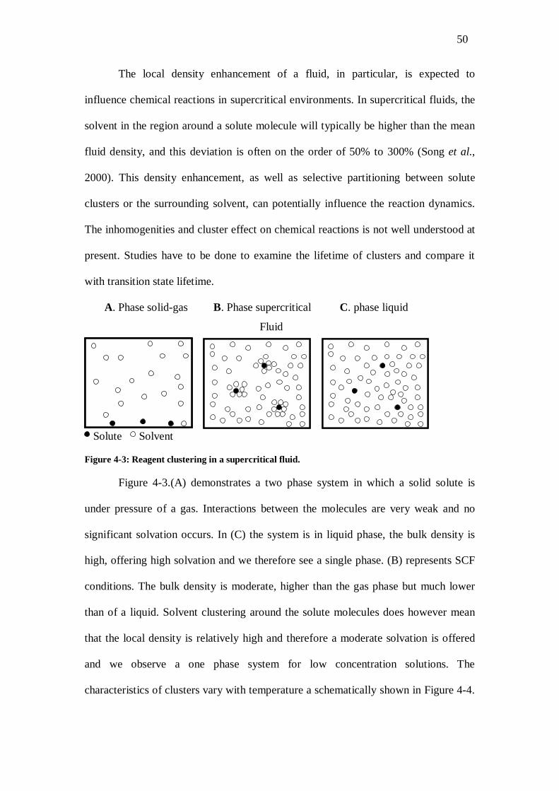
50

The local density enhancement of a fluid, in particular, is expected to

influence chemical reactions in supercritical environments. In supercritical fluids, the

solvent in the region around a solute molecule will typically be higher than the mean

fluid density, and this deviation is often on the order of 50% to 300% (Song et al.,

2000). This density enhancement, as well as selective partitioning between solute

clusters or the surrounding solvent, can potentially influence the reaction dynamics.

The inhomogenities and cluster effect on chemical reactions is not well understood at

present. Studies have to be done to examine the lifetime of clusters and compare it

with transition state lifetime.

A. Phase solid-gas B. Phase supercritical C. phase liquid

Fluid

Solute Solvent

Figure 4-3: Reagent clustering in a supercritical fluid.

Figure 4-3.(A) demonstrates a two phase system in which a solid solute is

under pressure of a gas. Interactions between the molecules are very weak and no

significant solvation occurs. In (C) the system is in liquid phase, the bulk density is

high, offering high solvation and we therefore see a single phase. (B) represents SCF

conditions. The bulk density is moderate, higher than the gas phase but much lower

than of a liquid. Solvent clustering around the solute molecules does however mean

that the local density is relatively high and therefore a moderate solvation is offered

and we observe a one phase system for low concentration solutions. The

characteristics of clusters vary with temperature a schematically shown in Figure 4-4.

51

Near the critical point at CT T , the solvent fluid molecules themselves are apt to

form clusters of extremely large size.

The effect of pressure on the rate of chemical reactions was originally revealed

in solutions under pressure (Asano and Lenoble, 1978; Tiltscher and Hofmann, 1987;

Vaneldik and Klärner, 2002). These researches were initiated much earlier than

researches in supercritical solvents. Elementary chemical reactions are generally

classified according to whether or not the reacting complex must surmount a potential

energy barrier in the course of reaction. Reactions for which this is true are called

activated processes, while those for which it is not are called diffusion controlled

processes. The features of supercritical fluids originate mainly from the

intermolecular interactions can affect both of the processes. It is obvious that the

study on intermolecular interactions in SCF is very important to their applications.

Figure 4-4: Different character of clusters formed in different temperature ranges. Near the critical temperature, the solvent molecules tend to form a large cluster even without a solute molecule. At higher temperatures, the solute molecule with strong attractive interaction is necessary to trigger the clustering of solvent molecules (Reprinted from Baker’s work (Baiker, 1999).

52

4.3 CARBON DIOXIDE

4.3.1 Background Although scCO2 has received much attention within academic and chemical

industrial laboratories both as a green alternative to conventional organic solvent and

as a simple, linear triatomic molecular system, the solvent behaviour of scCO2 is not

well understood on a microscopic level. The non-toxicity, low cost, abundance, and

ease of recycling are some of the key attributes of this environmentally benign

solvent. The low critical temperature of CO2 (Tc =31.1°C) ensures that scCO2 is a safe

solvent for biomolecular separations, pharmaceutical applications, and in other

thermally labile systems. CO2 is a major by-product in several industrial processes,

and in terms of availability, it is almost as readily abundant as H2O. Additionally,

because CO2 is recognized as a “green house” gas, recycling of by-product gas and its

industrial utilization are an important mode of reducing emissions into the

atmosphere. Over the past two decades, there are several areas where CO2 research

has progressed with developments in applications such as CO2-based dry cleaning,

polymer synthesis, extraction and separation of natural products, chemical

transformations, synthesis and dispersion of nanoparticles, and materials processing.

However, the large-scale utilization of this solvent suffers from the lack of a

molecular level understanding of the solvation phenomenon in CO2. How is CO2

classified as a solvent? What are the basic characteristics concerning solvation in

CO2, and how is it different from common solvents such as hexane and H2O? What

sort of molecular systems can CO2 dissolve, and what types of interactions

predominate? These are some of the important issues that need to be addressed before

it is possible to expand the use of CO2 as an industrial solvent.

53

Computational approaches provide excellent insight into understanding the

microscopic solute-solvent interactions, microscopic properties and microscopic

properties. The development of accurate computational studies for solute solubility

and reactions rates in liquid and supercritical carbon dioxide requires a model for

intermolecular interactions between this solvent and any solutes. Once a model for

carbon dioxide has been selected, it is important to characterize it with its predictions

of the equation of state, the liquid-vapour coexistence curve, and the critical

properties.

4.3.2 Equation of State for Carbon Dioxide The current standard National Institute of Standards and Technology (NIST)

equation of state for CO2 was developed by Span and Wagner (Span and Wagner,

1996). For reference, Table 4-2 gives the critical point and triple point conditions for

CO2. The critical temperature for CO2 is slightly above room temperature.

Table 4-2: Critical point and triple point for CO2. T/K P/MPa ρg/(Kg/m3) ρg/(Kg/m3)

Critical Point 304.128 7.3773 467.6 467.6

Triple Point 216.59 0.5180 13.73 1178.5

4.3.3 Models for Carbon Dioxide Most frequently, simulations of model fluids at near- and supercritical

conditions have been performed without the knowledge of the model’s vapour-liquid

equilibrium envelope, i.e., by simply taking the state conditions from the phase

diagrams of the real substances. The recent development of powerful new simulation

techniques for the direct determination of phase equilibria, such as the Gibbs

Ensemble Monte Carlo (Panagiotopoulos, 1987), the Gibbs-Duhem intergration

(Kofke, 1993), and the Grand Canonical Monte Carlo with histogram re-weighting

method (Kiyohara et al., 1998) make it possible to determine the phase diagram of

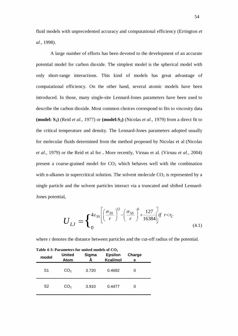
54

fluid models with unprecedented accuracy and computational efficiency (Errington et

al., 1998).

A large number of efforts has been devoted to the development of an accurate

potential model for carbon dioxide. The simplest model is the spherical model with

only short-range interactions. This kind of models has great advantage of

computational efficiency. On the other hand, several atomic models have been

introduced. In those, many single-site Lennard-Jones parameters have been used to

describe the carbon dioxide. Most common choices correspond to fits to viscosity data

(model: S1) (Reid et al., 1977) or (model:S2) (Nicolas et al., 1979) from a direct fit to

the critical temperature and density. The Lennard-Jones parameters adopted usually

for molecular fluids determined from the method proposed by Nicolas et al (Nicolas

et al., 1979) or the Reid et al for . More recently, Virnau et al. (Virnau et al., 2004)

present a coarse-grained model for CO2 which behaves well with the combination

with n-alkanes in supercritical solution. The solvent molecule CO2 is represented by a

single particle and the solvent particles interact via a truncated and shifted Lennard-

Jones potential,

12 6 1274 16384

0{

SS SSSS Cif r r

r rLJU

(4.1)

where r denotes the distance between particles and the cut-off radius of the potential.

Table 4-3: Parameters for united models of CO2

model United Atom

Sigma Å

Epsilon Kcal/mol

Charge e

CO2 3.720 0.4692 0

CO2 3.910 0.4477 0

S1

S2

55

Beyond the simple united atom approaches, there are three potential models designed

to fit the properties of CO2: a 2-point, a 3-point model and 5-point model. The “two-

center Lennard-Jones quadrapole” model developed by Möller and Fischer (Moller

and Fischer, 1994) fits empirical saturation data to two Lennard-Jones sites and a

quadraupole. The model of Möller and Fischer was used by Colina et al (Colina et al.,

2003) to describe the thermal properties of supercritical carbon dioxide, except in the

extend critical region. The Murthy (Murthy et al., 1983) potential was used by Iwai

group (Higashi et al., 2000) to describe the density dependence of structure of

supercritical carbon dioxide along an isotherm. The 5-point model of Murthy, O’Shea

and McDonald (Maillet et al., 1998; Murthy et al., 1983) uses three Lennard-Jones

sites and five Coulombic sites along the molecular axis. The “elementary physical

model” (EPM) of Harris and Yung (Harris and Yung, 1995) simplifies the 5-point

model by using three Lennard-Jones sites each with a Coulombic charge. The EPM

was optimized to get the correct pressure at 239 K, and it has a gas phase quadrapole

of 4.3 × 10−26 statcoulomb cm2 near the experimental value of 4.1 × 10−26 statcoulomb

cm2. The model is designed to be either completely rigid or have a flexible bond. The

rigid EPM fits the critical point within 3%. Harris and Yung rescaled the EPM using

corresponding states theory to obtain a model (EPM2) that matched the critical

properties of CO2. EPM and EPM2 use a combination Lennard Jones site and point

charge at each atom centre.

Table 4-4: Parameters for EPM2 and EPM model model Atom Sigma

ÅEpsilon Kcal/mol

Charge e

C 2.757 0.0559 +0.6512 eO 3.033 0.1600 -0.3256 e

C 2.785 0.0576 +0.6645 eO 3.064 0.1649 -0.3322 e

EPM2

EPM

56

Accordingly site-site interaction models are the most popular choice for

carbon dioxide. A number of the potential models for carbon dioxide can be regarded

as EPM based models. The first variation of the EPM model was proposed by Potoff

and Siepmann (Potoff and Siepmann, 2001) and is well known with the abbreviation

TraPPE. Zhang and Duan (Zhang and Duan, 2005) proposed another version of EPM

model by optimizing its parameters by obtaining a better predictability of phase

behaviour. Potoff (Potoff and Siepmann, 2001) proposed a model for carbon dioxide

with using only the term of power of six in Lennard Jones function, which shows

improved accuracies for the PVT properties at high densities. All of the EMP based

models have the angle of OCO fixed as 180o .Based on their structural experimental

studies, Zhang and Duan (Zhang and Duan, 2005) proposed a new molecular potential

abbreviated as EPM-M and EPM2-M with the only difference from EPM model the

intermolecular bond angle which is 174.2o. Up to date the EPM2 is the widely used

potential, although developed over ten years ago (Nieto-Draghi et al., 2007).

4.4 OTHER COMMON SUPERCRITICAL FLUIDS

4.4.1 Fluoroform

Fluoroform (CHF3) has a conveniently located critical point ( CT = 26.1°C,

CP = 4.8 MPa), is non-toxic and relatively benign to the environment, and is available

in high purity at modest cost. For these reasons, fluoroform has served as the

prototype for polar supercritical solvents in numerous experimental studies over the

past decade. Several simulation models of fluoroform have already been developed

(Hloucha and Deiters, 1998; Lisal and Vacek, 1996; Potter et al., 1997; Song et al.,

2002) and successfully applied to study a number of properties of the fluid (Okazaki

et al., 1995; Song et al., 2002). The model proposed by Song et al is a 2-site model

developed for use in simulations in the near critical regime. The model was optimized

57

to reproduce the critical point and the liquid-vapour coexistence curve of the real fluid

using the Gibbs Ensemble Monte Carlo method.

The model is a Lennard-Jones potential plus a Coulombic interaction (Song et

al., 2002). The 2-site model of fluoroform has been used by Song and Maroncelli

(Song and Maroncelli, 2003) to examine the role of electrostatic forces on density

augmentation on supercritical fluoroform.

Table 4-5: Model parameters of the 2-site model for CHF3 molecule. The distance between the 2 sites is 1.670 Å

site Sigma Å

Epsilon Kcal/mol

Charge e

1 3.500 0.1699 +0.275e2 3.500 0.1699 +0.275e

4.4.2 Ethane After methane, ethane is the second-largest component of natural gas. Ethane

is isolated on an industrial scale from natural gas, and as a by-product of petroleum

refining. Ethane is of great interest in separation industry. Many molecular potential

have been developed for ethane for different conditions, the most commonly used is

the UA-OPLS model developed by Jorgensen et al (Jorgensen et al., 1984) and

TraPPe model developed by Siepmann group (Martin and Siepmann, 1998). Ethane

(CH3CH3) has a critical point ( CT = 32.18°C, CP = 4.8718 MPa) close to fluoroform.

To date all of the developed potentials have been tested across their ability to predict

the critical point (Nath et al., 1998). The TraPPe model gives good agreement with

experimental critical properties. The 2-site model parameters of the TraPPe model are

given in the Table 4-6

Table 4-6: Model parameters of the 2-site model for CH3CH3 molecule. The distance between the 2 sites is 1.54 Å

site Sigma Å

Epsilon Kcal/mol

Charge e

1 3.750 0.1947 02 3.750 0.1947 0

58

4.4.3 Water Water at elevated and supercritical temperatures is found at the bottom of the

oceans as well as in electric power plants (Ulrich Franck, 1987). Supercritical water

(SCW) can be a suitable reaction medium for reactions usually carried out in organic

solvents. The SCW except the well-known advantages (Levert Sengers, 1998) using a

supercritical fluid as a reaction medium also influences the rates of chemical

reactions. During a reaction, the transition state may be higher or lower polarity than

the initial state. A high relative dielectric constant lowers the activation energy of the

reaction of a transition state of higher polarity than the initial state. By variation of the

relative dielectric constant, achieved by adjusting the temperature and pressure, the

reaction rates maybe controlled. As a consequence, these reactions show a high

activation volume. Fundamental chemical properties, which are well-known in

aqueous chemistry at 298 K, are much less available for SCW

( cT =647.13 , 30.322 /c g cm , 220.55 cP bar ) solutions (Reid et al., 1977).

Modelling the behaviour of water has been the subject of extensive research.

To describe the molecular structure of water, the most widely used effective pair

potential models use rigid multiple interaction sites with partial charges, such as the

three-site TIP3P (Jorgensen, 1981), SPC (de Pablo et al., 1990), and SPC/E

(Berendsen et al., 1987), the four-site TIP4P (Jorgensen et al., 1983), and the five-site

ST2 (Stillinger and Rahman, 1974) models, whose merits have been well documented

(Paschek, 2004). In particular, the three-site TIP3P, SPC, and SPC/E models are

commonly used in biochemical simulations, in part because of their reasonable

descriptions of solvation and dielectric properties. The model parameters for TIP3 are

given in Table 4-7 . The TIP3 have chosen to be used in this study, due to its

compatibility with EPM2.

59

Table 4-7: Model parameters of TIP3 model. model Atom Sigma

ÅEpsilon Kcal/mol

Charge e

H 0 0.0000 0.417 eO 3.151 0.1521 -0.834 eTIP3

4.4.4 Methane During the last two decades, the properties of fluid methane have been studied

by several groups using various experimental and theoretical techniques. The reason

for this long-lasting interest is that methane is the major constituent of natural gas.

Note that natural gas is one of the most promising fuels in reducing carbon dioxide

emissions. Further, it is much cheaper and environmental friendly than petroleum-

based fuels. Methane is one of the simplest polyatomic molecules. Its spherical

symmetry allows it to be modelled as a single site molecule with more accuracy than

almost any other polyatomic molecule. Modelled as a single site molecule the

majority of potentials for methane are based Lennard Jones potentials. The OPLS-UA

potential proposed by Jorgensen (Jorgensen et al., 1984) is the one widely is in use.

An alternative generic effective pair potential is given by the Bunckingham (Martin

and Siepmann, 1998) potential, but it is not easily compatible with Lennard-Jones in

case of mixture simulations.

Table 4-8: Model parameters of OPLS-AA model. model Atom Sigma

ÅEpsilon Kcal/mol

Charge e

H 2.500 0.0300 -0.24 eC 3.500 0.0660 0.06 eOPLS-AA

The most common used potential is the all-atom (AA) five-centre semi

empirical Lennard–Jones (LJ) potentials, with or without electrostatic interactions,

proposed by Jorgensen et al. (Jorgensen et al., 1996) and Murad–Gubbins (MG)

(Quirke and Gubbins, 1996), provide the most accurate description of the liquid

compared with other site–site potentials (Skarmoutsos et al., 2005). The OPLS-AA

60

model is choosen for this study as it is compatible with EPM2. Its parameters are

given in Table 4-8.

4.5 SUPERCRITICAL FLUID KINETICS

Chemical processes in SCFs can be controlled by a variety of factors, such as

enhanced transport coefficients, increased reactant solubilities, facilitated separation,

and strong “kinetic pressure” effect on the rate constants. For any given reaction,

several aforementioned factors can be affecting the reaction rate simultaneously,

which makes the analysis of chemical processes in SCFs rather involved. Therefore, it

is important to study simple, well-defined reactions, where it is possible to isolate a

few dominant factors influencing the reactivity. In this regard, the investigation of

chemical equilibria in SCFs provides a particularly appealing area of research, since

the values of the equilibrium constants are largely determined by the structural aspects

of supercritical solvation.

Pc

LS

V

Tc T

Figure 4-5: Schematic illustration of regions of the phase diagram; near-critical regime (dark area); compressible-regime (light dark area); supercritical regime (slanted hatch)

61

At present, however, the properties of SCFs and their effects on solute reaction are not

well understood, and the way is open for computation to provide the underlying

insight necessary for efficient development of SCF technologies.

When T exceeds Tc, there can be no phase transition between the vapour and liquid

phases. Instead, as the pressure is increased the fluid density is changed continuously

from gas-like to liquid-like densities. Consequently, density-dependent solvent

properties, such as the dielectric constant and the viscosity, will also vary

continuously. Pressure thus provides direct control of the fluid’s solvating properties.

This tunability is more effective when large changes in density accompany small

changes in pressure, i.e., when the isothermal compressibility is large. Coincidentally,

the compressibility of a fluid diverges as its critical point is approached, and there

exists a region of the phase diagram surrounding the critical point (with the restriction

that T>Tc) within which the fluid’s compressibility is anomalously large (Figure 4-5).

Evidentially, it is in this compressible regime that pressure-controlled tunability of the

solvent properties is maximised, and it is thus of primary interest to understand solute

reactivity in this solvent regime.

4.5.1 Effect of density on Equilibrium Constant

The effect of pressure (P) on reaction equilibrium constant (Kc), which is the

ratio of forward and reverse rate constants f rk k , is expressed in terms of the reaction

volume rxnV :

c rxnT i

T

K VP RT

(4.2)

For a general reaction

kf

kr γΓ + δΔ ... αΑ + βΒ ...

62

where i is the sum of the stoichiometric coefficients for the reaction, and T is

the isothermal compressibility. The reaction volume is defined as the sum of the

products of the stoichiometric coefficient and the partial molar volume iV for each

species in the reaction. The reaction volume is

( ...) ( ...)rxn A BV V V aV V (4.3)

The difficulty in using (4.2) and (4.3) with experimental data is that

experimental measurements of partial molar volumes are challenging (Guo and

Akgerman, 1998). Measuring partial molar volumes is very difficult because of the

problems associated with observing the supercritical phase the low concentrations and

short lifetimes of highly reactive species. An alternative approach to experimental

measurements of partial molar volumes or equilibrium constants is theoretical

determination of these quantities.

4.5.2 Effect of density on Kinetic Constant In conventional transition state theory, the pressure dependence of a rate

constant is related to the activation volume as it described by Equation (2.5)

#

,

ln (1 ...)C

T C

k VP RT

(4.4)

where T is the isothermal compressibility of the solvent. The activation volume is

calculated as the difference in the partial molar volumes of the transition state (“TS”)

and the reactants.

#TS A BV V aV V (4.5)

The partial molar volumes can be calculated like the equilibrium constant case from

the pair correlation functions for infinitely dilute mixtures.

63

4.5.3 Partial Molar Volumes When solutes are introduced into such a fluid, substantial solvent density

enhancements (clustering) or depletion (cavitation) are often observed around solute

molecules. Debenedetti and co-workers identified 3 solute behaviours: repulsive,

weakly attractive, and attractive, as follows (Debenedetti and Mohamed, 1989;

Petsche and Debenedetti, 1991).

1. Repulsive solutes are those for which the repulsive part of the solute-solvent

potential dominates the solute-solvent interactions. In this case, the solute and

solvent molecules repel each other and, consequently, the average solvent

density around a solute is less than the bulk density. Thus, addition of solute

increases the volume of the solution and gives positive partial molar volumes

(PMV).

2. Weakly attractive solutes are those for which the solute-solvent potential

interaction is dominantly attractive but are less so than the solvent-solvent

potential interaction. So, the addition of solute still increases the volume of the

solution and gives positive partial molar volumes.

3. Attractive behaviour results when the dominant solvent-solute interaction is

more attractive than the solvent-solvent interaction, so that the solute-solvent

correlations exceed the solvent-solvent correlations. In this case, addition of

solute decreases the volume of the solution and gives negative partial molar

volumes.

The observed partial molar volumes provided the main impetus for a whole

new realm of investigations seeking to better understand the intermolecular

interactions between the solute and the other species in SCF solutions. For example

the partial molar volume of naphthalene at infinite dilution in a mixture of

naphthalene and supercritical carbon dioxide is -2300cm3/mol at P=76 bar and

64

T=308.38 K (Eckert et al., 1986), while the partial molar volume of ethane at infinite

dilution in a mixture of ethane and supercritical carbon dioxide is +350 cm3 /mol at

P=73.97 bar and T=305.65 K. According to the classification of Debenedetti and

Mohamed the above mixtures (CO2/naphthalene and CO2/ethane) belong to different

types of supercritical mixtures; CO2/naphthalene is an ‘attractive’ mixture and

CO2/ethane is a ‘weakly attractive’ mixture.

The research group of X.Zhang (Zhang et al., 2002a; Zhang et al., 2002b)

reported new data of PMVs of solutes in dilute supercritical solution. In their study,

the PMVs of two polar solutes (H2O and H2S) in supercritical CO2 are negative, and a

minimum can be observed in each PMV versus pressure curve at the pressure where

isothermal compressibility of the fluid is largest. On the opposite site the PMVs of

two non-polar solutes (H2 and CH4) are positive.

For a solute (u) in solvent (V), the partial molar volume is defined as

, V

u

u pT n

VVn

(4.6)

with nu and nV being the numbers of moles of the solute and solvent, respectively. At

infinite dilution, V

u u u s u sp,T,n0V = lim n V(n =1,n ,T,P)-V(n =0,n ,T,P)

un

, so uV can

be computed in the isothermal-isobaric ensemble (NPT) from Monte Carlo

simulations (Iwai et al., 1997). The computational method is not limited to Monte

Carlo simulations; molecular dynamics simulations are equally applicable. Partial

molar volume studies have been reported with this method (Stubbs et al., 2005) for

naphthalene carbon dioxide mixture near the critical point with reasonable accuracy.

An alternative approach is to use the Kirkwood-Buff (KB) fluctuation theory

(Kang and Smith, 2007). This theory and its extension have been applied to study

dilute supercritical fluid mixtures (Akiya and Savage, 2000a; Akiya and Savage,

65

2000b; Chitra and Smith, 2001a; Chitra and Smith, 2001b; Lin and Wood, 1996). In

this formalism, the partial molar volume at infinite dilution can be calculated as

01 ( )v uv vvV G G (4.7)

where Guv and Gvv are solute-solvent and solvent-solvent fluctuation integrals,

respectively. The subscript u refers to the solute and v to the solvent. The superscript

0 and refer to the pure solvent or infinitely dilute co-solvent, respectively. These

fluctuation integrals are a function of pair correlation functions (gij(r)):

2

04 ( ) 1ij ijG g r r dr

(4.8)

Thus partial molar volumes depend on the relative strengths of the solute-solvent and

solvent interactions. Pair correlation functions can be calculated directly from

molecular simulations.

The KB theory relates fluctuations in particle densities in the grand canonical

ensemble to thermodynamic properties of mixtures. The pair correlation function or

radial distribution function (RDF) can be calculated through simulations in canonical

ensemble. The values of the integrals though RDFs can be obtained for

a. solvent-solvent

b. solvent-solute

c. solute-solute

The same integrals can be calculated for solvent and co-solvent, for mixture where we

don’t have diluted solutions with introducing some modifications.

4.5.4 Isothermal Compressibility The way in which the volume of a material decreases with pressure at constant

temperature is described by the isothermal compressibility, κT. Isothermal

compressibility is one on the important properties of the fluid, which gives very

66

strong indication of the unusual behaviours at supercritical conditions. The isothermal

compressibility (κT) can be obtained from densities of the fluids according to equation

(4.9)

T1 1

T T

VV P P

(4.9)

The theory of critical phenomena (Tucker and Maddox, 1998) tells us that, as the

critical point of a fluid is approached (T → Tc), the isothermal compressibility

diverges (i.e., it becomes infinite). Since this divergence occurs smoothly, there must

exist a region of the phase diagram with T > Tc for which the compressibility is

large, by which we mean that T > 0T , where κ is the compressibility of an ideal gas

(The compressibility of a perfect gas is given as 0T ). As it turns out, this region of

large , which is called the‘compressible regime’ extends well beyond the near-

critical region of the phase diagram in which all fluids behave universally and the

theories of critical phenomena apply (Tucker, 1999).

Macroscopically, a large compressibility means that there is very little cost

associated with an increase in solvent density, so we can easily compress the fluid.

From a molecular point of view, a large compressibility means that there is enough

free space, (a big voidage) between molecules, allowing the system to be compressed.

In this case, there are two pictures of molecular microstructure that can satisfy this

situation. Firstly, if the voidage is uniformly distributed between the molecules, or

secondly, if there are high and low density regions. In the first case, a little effort is

required to compress and condense the molecules together. In second case, a little cost

is required to transfer a molecule from a low-density region to a high-density one.

According to Morita (Nishikawa and Morita, 2000) there is a ridge that separates the

supercritical region into more liquid-like and more gas-like regions in the supercritical

67

region. The ridge is shown in Figure 4-6. According to their research group, the ridge

is the locus of the points where the values of the density fluctuation becomes

maximum in isothermal changes.

Pr = 1.1

ρc

SCF

L

V + L

V

Tc

Figure 4-6: The gas–liquid coexistence curve. The blue colour indicates a high density region (liquid like) and the red colour a low density region (gas like). The dashed line represents the locus of the points with the maximum local densities fluctuation (drawn on data representing vapour-liquid curve for carbon dioxide).

Density fluctuation and correlation length are quantitative expressions of the

static structural fluctuation from the standpoints of number of molecules and size of

molecular aggregates, respectively. The isothermal compressibility obtains its

maximum value on the locus of the points of ridge. The isothermal compressibility is

related to the Gibbs free energy through the equation

2

T 2

1 1

TT

G VV P V P

(4.10)

Many physicochemical properties of supercritical fluids are related to the

second derivative of the Gibbs or Helmholtz free energy, so we expect a unique

behaviour on the ridge. From this point of view, little work has been done connected

rate constants, equilibrium properties or solubilities with the ridge. However, rate

68

constants or equilibrium constants of various chemical reactions in supercritical fluids

show a singular behaviour on the ridge (Ikushima et al., 1992). Also infinite solution

studies reported an anomalous behaviour of solute partial molar volumes at pressures

where the ridge located (Guo and Akgerman, 1998).

4.5.5 Diffusion The most commonly used description of diffusivity on a quantitative basis is

via the measurement of the well-known self diffusion coefficient. The diffusion is the

rate of transfer of diffusing molecules through unit area of a section and is

proportional to the concentration gradient

( )CJ Dx

(4.11)

where D is the self diffusion coefficient. The self-diffusion is a single particle

property and can be obtained from molecular simulation dynamic simulations with

great accuracy. The common form to derive the diffusion coefficient through

molecular dynamics is the through the Einstein equation. Detailed explanation for the

intuiting aspect of the diffusion coefficient at supercritical conditions is given in the

results section of diffusivity.

69

Part II. Simulation

70

5 COMPUTATIONAL METHODOLOGY

olecular simulation has reached a stage where it can be reliably used

for a large array of equilibrium and non-equilibrium properties of

molecular liquids. The purpose of this chapter is to present the

technical details of the Monte Carlo simulation and molecular dynamics.

The two most widely used methods for atomic-level modelling of fluids

Monte Carlo statistical mechanics and molecular dynamics have been used in our

studies in the supercritical region. Both procedures typically have the same system

setup including representation of molecules as collections of atom-centred interaction

sites, utilization of classical force fields for the potential energy terms, and

implementation of periodic boundary conditions. The principal differences are in the

modes of sampling the configuration space available to the system. For MC, a new

configuration is generated by selecting a random molecule, translating it, rotating it.

Acceptance of the new configuration is determined by the Metropolis sampling

algorithm; application over enough configurations yields properly Boltzmann-

weighted averages for structure and thermodynamic properties. For MD, new

configurations are generated by application of Newton's equations of motion to all

atoms simultaneously over a small time step to determine the new atomic positions

and velocities. In both cases, the force field controls the total energy (MC) and forces

(MD), which determine the evolution of the systems. In our simulations, we used both

of the methods.

M

71

5.1 INTRODUCTION

Typically, a molecular system simulation is carried out with anywhere from 10

to 100,000 molecules. Larger systems are generally prohibited due to memory

requirements, and (more importantly) speed considerations. Force calculations

increase with number of particles. However, because we are using a very small

number of particles and trying to determine macroscopic properties one must be very

careful that the results are not system size-independent. Unless the actual system

being studied is very small (a droplet, microstructure etc) a simulation box with 1000

molecules will have a disproportionate number (nearly half) of molecules at the

“surface”. This would completely skew the behaviour of the system. In order to get

around this problem, we employ a trick called periodic boundary conditions. In this

model, one chooses a small part of the full system to simulate and then makes the

assumption that the rest of the system can be modelled as an infinite series of copies

of the central box. This consideration of periodicity makes the simulation of

condensed phase systems applicable.

5.2 PERIODIC BOUNDARY CONDITIONS

In the periodic boundary condition approximation, an infinite system is

constructed as a periodically repeated array of the finite system that is being studied.

A schematic diagram of a two-dimensional system is shown in Figure 5-1, each

replica containing the same number of molecules in the same configuration (positions

and orientations). Thus when a molecule moves through a boundary and so out of the

sample it is automatically replaced by a molecule moving into the sample through the

opposite face of the box.

72

1 1 12 3 I=3 2 3 I=3 2 3 I=3

4 8 4 8 4 86 6 6

5 7 5 7 5 79 9 9

1 1 12 3 I=3 2 3 I=3 2 3 I=3

RC

4 8 4 8 4 86 6 6

5 7 5 7 5 79 9 9

1 1 12 3 I=3 2 3 I=3 2 3 I=3

4 8 4 8 4 86 6 6

5 7 5 7 5 79 9 9

Figure 5-1: Schematic representation of periodic boundary conditions for two–dimensional system

Anyone who has played video games such as Pacman, Asteroids, Galaxians etc. will

be familiar with this periodic boundaries trick. The primary simulation box can be

envisioned as being surrounded by images of itself; for a “cube”, there would be 26

images around the central box. The central box is the “unit cell”. With such periodic

boundaries it is only necessary to store the coordinates of the molecules in the central

box, the periodic images being copies of these.

Here we have to repeat that the heart of a Monte Carlo simulation program

is the calculation of the energy. However, the assumption of periodicity immediately

makes the simulation of such system tractable even through all the molecules in it are

modelled explicitly.

In order to calculate the intermolecular interaction of any molecule, we

position it at the centre of a box with dimensions identical to the simulation box. The

73

central molecule interacts with all molecules whose centres fall with this region, i.e.,

the closest periodic images of the other N - 1 molecules. The simplest procedure is to

use a spherical cutoff such the interactions are evaluated with the nearest images of

the other molecules out to a cutoff distance RC, as illustrated in Figure 5-1. In order to

avoid evaluation of interactions with more than the one image of another molecule RC

is always chosen to be less than or equal to half the length of the shortest edge of the

periodic cell. Typically, values for RC are 10-15Å. Historically, an alternative

approach with a cubic cutoff was used occasionally used whereby the interactions

were evaluated with the nearest image of each of the remaining N-1 molecules. This

procedure was abandoned since the boundary conditions do not reflect the normal

spherically symmetric nature of the intermolecular forces and it requires the

calculation of roughly twice as many pair interactions as spherical cutoff. The

spherical cutoff is an approximation that could (and does) have important

consequences for the behaviour of a system during a molecular simulation. It would

be obviously better to have methods that allow the interaction after the cutoff to be

considered. A class of such approximations exists and they are called long range

corrections techniques.

5.3 CONFIGURATIONAL ENERGY

The potential energy controls the outcome of the Monte Carlo simulations. It

is computed from the pairwise sum of the intermolecular interaction energies between

molecules. Because our studying systems comprised of small molecules, we shall

restrict ourselves to treat the molecules as rigid molecules and we will ignore the

intramolecular interactions. So the intermolecular interaction is restricted to pairs of N

molecules and total potential energy (U) is obtained by summing over the contribution

all of the individual pairs.

74

1

1 1IJ

N Imol

I JU U

(5.1)

This calculation is known as Naïve Energy Calculation (Sadus, 2007), it is

obvious that the “self” interactions do not contribute to the potential energy of the

system and we avoid the “double” calculation of the pair interactions. Obviously, the

type and nature of the terms in the energy function and the values of the parameters

will depend upon the force field that we choose to use.

To model intermolecular interactions, we adopt pairwise additive effective

potentials of the sort commonly employed in computer simulation. Specifically, the

interaction between two molecules I and J is assumed to be given by the sum of site-

site terms of the Lennard-Jones plus Coulomb form

12 6

44

i j ij ijij

i I j J o ij ij ij

q qU

r r r

(5.2)

where εο=8.8541910-12C2N-1m-2 is the dielectric constant of the vacuum, iq is

the charge on site i of the molecule I, ijr is the distance between sites i and j, and ij

and ij are Lennard-Jones interaction parameters between sites i and j located at

molecules I and J. Sometimes simulation models involve with united-atom (UA)

(Jorgensen et al., 1984) representations wherein multiple atoms are combined into a

single interaction site or all-atoms (AA) versions (Jorgensen et al., 1996).

For the Lennard-Jones interactions between unlike atoms, the Lorenzt-

Berhelot combining rules were used. The Lennard-Jones interactions were calculated

using the arithmetic mean of the core diameters and the geometric mean of the well

depths.

2

i jij

(5.3)

75

ij i j (5.4)

The exact form of the energy within the cutoff distance is given by the form below

12 6

1

1 14

4

Nmol Ii j ij ij

ijI J i I j J o ij ij ij

q qU

r r r

(5.5)

5.4 LONG RANGE CORRECTIONS

So far, we have discussed the concept of periodic boundary conditions and the

output for the configurational energy. In all these theories we assume “perfect”

structure. Although, we know that real materials do have order and structure,

particularly on short length scales. The basic idea behind this concept is that,

elucidation of the structure of fluids is important to understanding fluid behaviour.

Considering Figure 5-2, which represents a snapshot of a collection of spherical

molecules, with an arbitrary particle picked as a reference. At a distance r from the

reference particle, the density of other particles )(r will depend on time. However,

on average the density will be a quantity dependent only upon distance, r

dr

Figure 5-2: Typical arrangement of a fluid of spherical particles. The density at a given radius r with respect to a reference particle is shown.

We can immediately recognize several qualitative features from Figure 5-2.

First, )(r must tend toward zero, as r goes to zero, since additional particles cannot

occupy the same location as the reference particle. Second, at large r, the influence of

76

the reference particle is zero, and )(r must approach , the macroscopic density.

Third, at intermediate separations, )(r may be less than or exceed , depending on

whether the distance r corresponds to distances of repulsion or attraction between

particles.

Now, we define a function /)()( rrg the behaviour of g(r) is such that

0)( rg as 0r

1)( rg as r

g(r) is called the radial distribution function.

We mentioned that the Monte Carlo algorithm it depends on the outcome of

the total energy. The potential energy is defined as

IJU U (5.6)

The differential number of molecules rdN in an element of spherical volume at a

distance 2dr 4 drr between r and r + dr from the central molecule is

2rdN g(r)4 dr (5.7)

The potential energy of this differential system is

2IJU (r)g(r)4 dr (5.8)

For all distances from the reference molecule, the total potential energy is

2IJ

0

U (r) (r)g(r)4 dr

(5.9)

What about the portion of the potential energy that was “cut off”? The

contribution to U from the truncated “tails” of the pair potential function (the so–

called “long range correction”) is calculated by direct integration, using the energy

equation. To obtain the total potential energy of the system, we would sum over all

molecules, letting each one be the reference. Each integral would be the same as the

77

above expression. Thus, we would expect that the total internal energy would be

obtained by multiplying the above expression by N, the total number of molecules.

However, this would over count, since each pair interaction would be counted twice.

Consequently, fullU is obtained from

C

12

full c lrc1 1 R

U U U 2 V(r)g(r)r drmolN I

IJI J

U N

But how strong are these long range interactions and what part of the total part

of energy they account of?. Let’s have a look on the EPM2 model for carbon dioxide.

The EPM2 model is presented in Figure 5-3

180 ο

LJ Carbon σ =2.785 Α ε =0.0576 Kcal -0.33225 e

-0.33225 e +0.6645 eLJ Oxygen σ = 3.064 Α ε = 0.16493 Kcal

Figure 5-3: Parameters for EPM2 model for carbon dioxide. The distance between carbon and oxygen at 1.149Å

The influence of the potential never vanishes for electrostatic interactions.

Therefore, it is clear that the treatment of long-range electrostatic interactions must be

performed. Long-range Van der Waals interactions are less strong and decay more

quickly with distance.

The Coulomb potential vanishes as 1/r, which is a much slower decay than the

1/r6 dispersion interaction characterized by the LJ model potential. Representative

curves are shown in Figure 5-4 and Figure 5-5. Whereas the LJ model can quite

reasonably be truncated at about 2.5 LJ diameters, the Coulomb potential is at five LJ

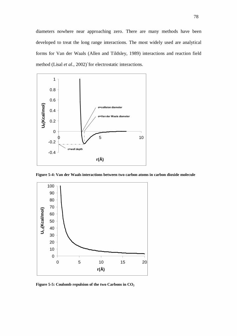
78

diameters nowhere near approaching zero. There are many methods have been

developed to treat the long range interactions. The most widely used are analytical

forms for Van der Waals (Allen and Tildsley, 1989) interactions and reaction field

method (Lisal et al., 2002)`for electrostatic interactions.

-0.4

-0.2

0

0.2

0.4

0.6

0.8

1

0 5 10

r(Å)

U E(K

cal/m

ol)

σ=collision diameter

ε=well depth

σ=Van der Waals diameter

Figure 5-4: Van der Waals interactions between two carbon atoms in carbon dioxide molecule

01020304050

60708090

100

0 5 10 15 20

r(Å)

ULJ

(Kca

l/mol

)

Figure 5-5: Coulomb repulsion of the two Carbons in CO2

79

5.4.1 Van der Waals interactions It is known that long range contributions have a significant influence on the

simulation of inhomogeneous systems, even with large number of molecules used in

the simulation.

Figure 5-6: A two dimensional diagram of an inhomogeneous system. In the κΩ physical space there, M elements interact with elements with the other elements of different physical spaces

For an inhomogeneous fluid system, the total long range corrections (LRC) LRCX to

an extensive thermodynamic property X is estimated in terms of all the local values

LRCX

1

( )M

LRC LRCk

X x

(5.10)

where is the physical space occupied by the κth local element having a uniform

density and M is the total number of local elements, like the Figure 5-6. In the

presentation of Figure 5-7, the term LRC refers to the LRC from Van der Waals

interactions. For a molecular system, the LRC to the Van der Waals configurational

energy of a molecule i interacting with molecules (molecule j) in the κth element, is

expressed by

80

,

1( , )

th

MLRC LRCi ij

kU u i dV

(5.11)

where , ( ) ( )th

LRCij ij j th

dV

u u r dV dV

.

The ( )j thdV is the density of the fluid in a volume element dV away from the

central molecule i in the κth local region, ( )iju r is the pair potential function, r is the

distance between the central molecule i and another molecule j in dV .

kth

jji

Rc

dV

Figure 5-7: The molecule i interacts with the molecules in the molecules within the kth element, volume dV. The element is outside the cutoff and Rc is the cutoff.

Assuming a homogeneous system, j is equal to bulk density , so we can recover

the standard expression for long range corrections to the energy of molecule i used in

bulk simulations by evaluating following integral:

2 9 38 84 ( ) ( )9 9i c c

rc

U r u r dr r r

(5.12)

The assumption is valid for our system as the potential function ( )u r decays very

quickly.

81

5.4.2 Electrostatic interactions Although the Ewald summation method can be used to estimate the long-range

electrostatic interactions with results similar to that the reaction field method (Hirst,

1985; Kettler et al., 2002; Lisal et al., 2002), it is computationally expensive.

Therefore, the reaction field method is selected to handle the long-range electrostatic

forces in this work. In this method, the long range corrections is given by

2 2

3 3

1 11 12 1 2 1

rf ij rf cutCoul i j

i I j J ij rf cut cut rf cut

r rU q qr r r r

(5.13)

where i and j are the interaction sites on two different molecules I and J respectively,

rf and cutr denote the reaction field dielectric constant and the cutoff distance,

respectively. rf is assumed to be infinity and this conducting boundary ( rf )

leads to both reasonably consistent results and good computational efficiency.

82

6 COMPUTATIONAL IMPLEMENTATION

n this chapter, technical details of the Monte Carlo and molecular dynamics

simulations are presented. We describe the approach used to perform Monte

Carlo simulation in terms of code developing. Programs to accomplish

simulations were all written in the programming language FORTRAN 90 and they

were then executed on some full-size servers like C3, Xenon, Plato and Socrates at

University College London. Modified modules from the Dynamo library (Martin and

Martin J.Field, 2000) and modified programs from Allan and Tildsley’s book (Allen

and Tildsley, 1989) were used to support the code development. The NAG compiler

was utilized to run the programs on these servers.

I

83

6.1 ALGORITHM DEVELOPMENT

The algorithm below describes the Monte Carlo pseudo code in canonical

ensemble. The code developing was a rigorous task, since the MC simulation needs

enough space and time even for a single run. In order to describe the code developing

we give below an overview of the primary parts of the code scheme.

Part 1 Initialisation: Assign initial coordinates rxi, ryi, rzi for the N atoms, N, V, T. Evaluate and store UTotal

Part 2 Production: Generate Markov Chains Assign values for Ncycles, Nsteps. loop n ← 1…NCycles loop n ← 1…Nsteps

Part 2.1 Generate a trial position: rxTrial ←(rxi + rMax x (2 x rand() -1)) ryTrial ←(ryi + rMax x (2 x rand() -1)) rzTrial ←(rzi + rMax x (2 x rand() -1))

Part 2.2 Calculate energy of molecule i at the trial position: (Utriali)

Part 2.3 Calculate change in the energy: ∆U ← Utriali – Ui

Part 2.4 Apply acceptance criterion: if (∆U < 0) ! accept new position rxi ← rxTrial ryi ← ryTrial rzi ← rzTrial Ui ← Utriali Utotal ← Utotal + ∆E ! update energy. else BF ← exp(-kB ΔU) ! Boltzmann factor if (BF > rand()) ! accept new positions rxi ← rxTrial ryi ← ryTrial rzi ← rzTrial Ui ← Utriali Utotal ← Utotal + ∆U !update energy. end if end if if (n > NEquilibrium) !end of equilibrium period

Part 3 Accumulation :Accumulate averages end if end i loop End n loop

84

An explanation of each part displayed in the algorithm is given in the next three parts

initialization, production and accumulation.

6.2 INITIALIZATION

The initialization procedure is consisting of two steps. The first one is building

the simulation box and the second one, calculating the total potential energy of the

system.

6.2.1 Solvent Box It is very important, how we are creating the first simulation box. The

approach adopted for the determination of the coordinates of the molecules in the box

is to start off by placing molecules at random within a box much larger than a box of

the target size. The coordinates of atoms are stored in a large Fortran 90 array:

ATMCRD (1:3, 1:NATOMS).

The size of the large box is then gradually reduced until the target size is

reached. The reason for starting off with a large box size is that the probability of

having molecules overlap will be small. The initial box length was ten times the target

length and the reduction procedure was carried out in ten steps. The number of ten

steps has been chosen arbitrary, the more steps the better is but they increase the

computational time. After the reduction procedure, the solvent box will have attained

the desired volume but the molecules will be by no means fully equilibrated. Thus, the

procedure finishes by performing a long Monte Carlo simulation, before writing out

the final coordinates to an external file. The coordinates of the last file can be

considered as an equilibrated box. Molecular dynamics can be used for the

equilibration of the initial box. A different approach is to start all the molecules from

a lattice. As moves progress, the lattice “melts” and a simulation box is obtained. The

initial period of the simulation is an equilibration period, and must be discarded. We

85

know that the final result should be independent of the starting configuration, so we

checked this by checking the results with using different initial boxes.

As pointed out before, the choice of number of molecules is crucial for the

calculation of any thermodynamic property. We choose to use 1000 solvent molecules

as a solvent box. The number 1000 is chosen as it is sufficient to describe the system

and efficient for keeping down the computational time. Furthermore, other research

groups use relevant amount of particles at similar conditions (Song and Maroncelli,

2003).

6.2.2 Potential Energy The calculation of the potential energy is crucial for the Monte Carlo

procedure. As we mentioned in the previous chapter, the energy is calculating by

adding the energy of pairs of particles. If intermolecular interaction is restricted to

pairs of N molecules, the total potential energy is obtained by summing over the

contribution all of the individual pairs. A pseudo-code scheme for the calculating the

total energy is given below:

loop i 1 ... N

loop j 1 ... i-1

Evaluate rij.

Evaluate u(rij).

Accumulate energy.

end j loop

end i loop

The above pseudo code illustrates the nesting of loops required for the Naïve

evaluation of energy by equation (5.1). If there are N molecules in the simulation,

then to calculate the pairwise energy experienced by each other molecule involves a

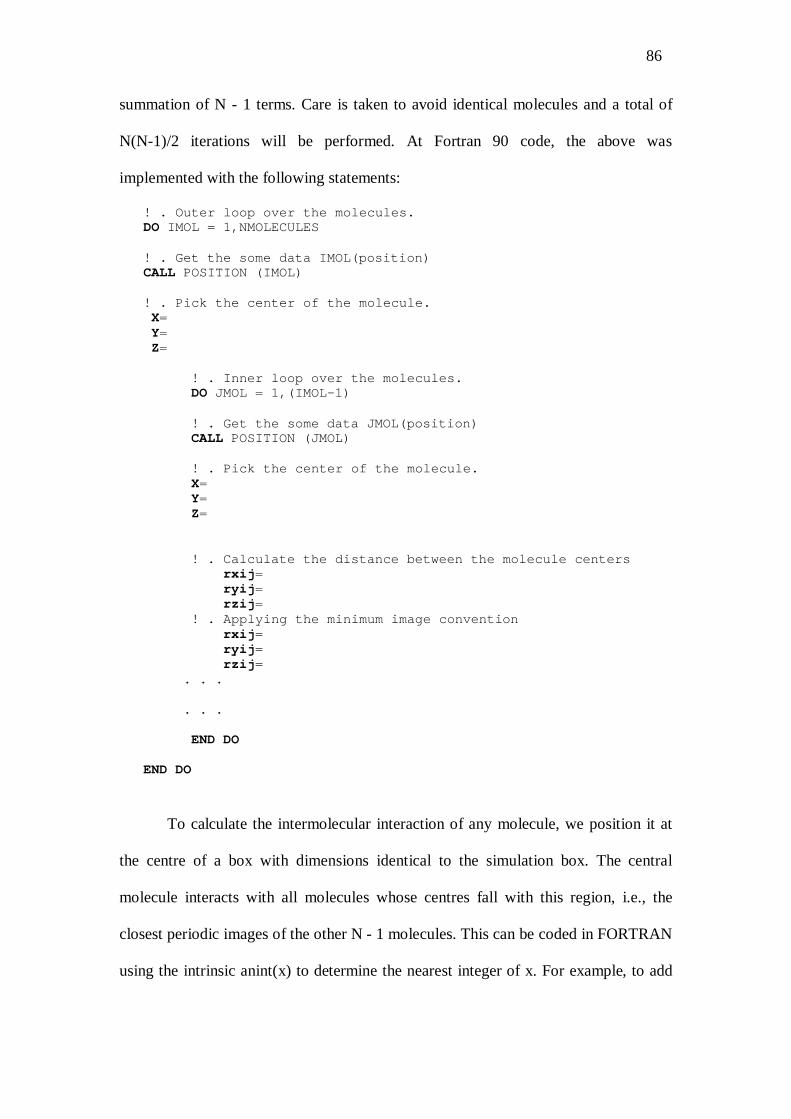
86

summation of N - 1 terms. Care is taken to avoid identical molecules and a total of

N(N-1)/2 iterations will be performed. At Fortran 90 code, the above was

implemented with the following statements:

! . Outer loop over the molecules. DO IMOL = 1,NMOLECULES

! . Get the some data IMOL(position) CALL POSITION (IMOL)

! . Pick the center of the molecule. X= Y= Z=

! . Inner loop over the molecules. DO JMOL = 1,(IMOL-1)

! . Get the some data JMOL(position) CALL POSITION (JMOL)

! . Pick the center of the molecule. X= Y= Z=

! . Calculate the distance between the molecule centers rxij= ryij= rzij= ! . Applying the minimum image convention rxij= ryij= rzij= . . .

. . .

END DO END DO

To calculate the intermolecular interaction of any molecule, we position it at

the centre of a box with dimensions identical to the simulation box. The central

molecule interacts with all molecules whose centres fall with this region, i.e., the

closest periodic images of the other N - 1 molecules. This can be coded in FORTRAN

using the intrinsic anint(x) to determine the nearest integer of x. For example, to add

87

the correct number of box lengths to the molecular coordinates rij or the pair

separation vector, we write:

rxij(i) = rxij(i) - boxl * anint( rxij(i) / boxl )

The above statement is evaluated in the loop, during the evaluation of energies. The

procedure for calculating the energy using periodic boundary conditions is given

below.

loop i 1 ... N

loop j 1 ... i-1

Evaluate rij.

Convert rij to its periodic image (rij).

if (rij< cut_off_distance)

Evaluate u (rij').

Add corrections to energy.

end if

end j loop

end i loop

The above algorithm is different from the naïve approach in two important respects.

a) The accumulated energy is calculated for the periodic separation

distances. Secondly,

b) Only molecules separated by a distance less than the cut-off distance

contribute to the calculated energy or forces.

The cut-off distance is a consequence of the periodic boundary conditions. It

can be any distance up to half the length of the simulation box. A higher cut-off is not

permitted because it would violate the minimum image convention. Consequently, the

above algorithm evaluates the properties of a truncated intermolecular potential rather

88

than the full potential. When PBC are used, the full contributions of the

intermolecular potential have to be obtained by using long-range correction terms.

The full energy was obtained by adding the long-range correction. The contribution of

the long-range correction was implemented into the loops though equations (5.12) and

(5.13).

6.3 PRODUCTION

The Monte Carlo simulation was performed in blocks (Part 2).Every block

consists of number of steps. During each step, a displacement and rotation is

attempted for every molecule (Part 2.1). The molecule to be displaced is chosen

randomly. It also possible to displace every particle and apply the acceptance criterion

to the combined move. This procedure has not been chosen, as it increases

dramatically the computational time. The displacement of the molecule is coding

though:

1. Choosing a molecule at random.

Choosen= INT ( NMOLECULES * rand(iseed))

Essentially, the above statement multiply the number of molecules

(NMOLECULES) with a random number (rand(iseed))and the INT function

converts the result to an integer.

2. Displacing the molecule.

rxtrial = rx(i) + (2.0 * rand(iseed) - 1.0) * drmax rytrial = ry(i) + (2.0 * rand(iseed) - 1.0) * drmax rztrial = rz(i) + (2.0 * rand(iseed) - 1.0) * drmax

where drmax a parameter, controls the “length” of the attempted,

rand(iseed)is a function for generating random number between 0 and 1.The rand is

equal to the fuction RANDOM_NUMBER()in Fortran 90. The iseed is the starting

number for random generator. After a displacement is made, the energy of the new

89

state is compared to the energy of the old state. The Metropolis selection rule is used

to decide whether or not this new state is accepted

6.4 ACCUMULATION

After the equilibration time, it is important that the successive values of any

observable be statistically independent when calculating mean fluctuations around

average values. So the calculations are often carried out in series of blocks (Nblocks)

containing a number of m steps (Nsteps). As the number of configurations (steps) in

each block increases, it would be expected that the block averages become

uncorrelated and successive values become independent. We monitored the potential

energy U by plotting in MS excel (see Figure 7-5). A schematic diagram of evaluation

of potential energy is given at Figure 6-1.

Figure 6-1: Schematic representation of potential energy during the Monte Carlo progress

6.5 TECHNICAL DETAILS

MC simulations were carried in the canonical ensemble (NVT) using periodic

boundary conditions. A system with the 1000 molecules was studied at all times.

t

U

Equilibration

90

Simulations were organised in cycles, each cycle consisting of 100000 attempts to

displace or rotate a randomly chosen molecule. A variable spherical cut-off radius,

equal to half the box length was used and long-range corrections were recalculated

after each move. Acceptance ratio of all trial moves was adjusted to 40%. In each run,

more than 107 Monte Carlo configurations were generated to reach equilibrium and

the structural and thermodynamic properties were obtained from the following 200 x

106 MC moves. We have studied three systems, ethane, fluoroform and carbon

dioxide. Details about the potential are given in results section. The main program is

given in appendix.

In all MD simulations, a spherical cut-off equal to the half of the simulation

boxed is used. A time step of 2 femtosecond is used in leapfrog verlet algorithm with

Berendsen thermostat (Allen and Tildsley, 1989). A time period equals to 0.5

nanoseconds is used for equilibration and 1.5 ns for production.We have studied three

systems, pure carbon dioxide, mixture of methane + carbon dioxide at infinite dilution

and water + carbon dioxide at infinite dilution. All simulations were performed at

temperature 308.15 K (Tr=1.02) in NVT ensemble. When in the text we refer to

solvent, we mean carbon dioxide except when we state differently and when we refer

to solute either to methane or to water. The methane molecule was represented by

OPLS-AA potential model and water by TIP3 model (see section 4.4.3 and 4.4.4).

The main program is given in appendix.

Rigid molecules are being used in the simulations. The geometries of water

molecule is the same with H-O bond distance of 0.9572Å and H-O-H bond angles of

104.52o. The methane molecule has tetrahedral symmetry, with C-H bond lengths of

1.090 Å and H-C-H bond angles of 104.47o.

91

92

Part III. Results and Discussion

93

7 RELIABILITY OF THE METHOD

here are two elements required to successfully predict physical properties

in molecular simulation. The first part requires the development of

appropriate molecular simulation techniques, in order to describe a

physical system as efficiently as possible. The second part is the development or use

of a suitable interaction potential model. Given the two perquisites, physical systems

can be described successfully.

In this chapter, we evaluate the outcome of our Monte Carlo program by

presenting the analogous results. Then, we are examining the validity of the molecular

potential in the supercritical region for supercritical carbon dioxide. In this study, we

have used a semi-empirical classical potential for carbon dioxide. It is an atomistic

model, which is mimicking carbon dioxide geometry and quadrupole momentum. It is

well known with the abbreviation EPM2 (Harris and Yung, 1995) and its parameters

are adjusted to reproduce the vapour-liquid curve.

T

94

7.1 INTRODUCTION

Examining the supercritical phase, in the vicinity of the critical temperature

(Tc1.01-1.103) though molecular modelling techniques, is a rigorous task for three

reasons. Firstly, there are few experimental data because of the problems associated

with observing the supercritical phase experimentally, in order to be compared with

computational studies. Clearly, without a comparison to experiment, the accuracy of

simulation results cannot be gauged.

Secondly, molecular simulation requires very large simulated systems (number

of molecules-simulated box) because the correlation length of the system becomes

macroscopic as the critical point is approached (Quirke and Gubbins, 1996), which

makes simulation run’s time consuming and approximations necessary on the

estimation of long range interactions. Surely, the rapid growth of computers has

provided scientists and engineers great advances in computational power, and has

made solving of numerous variable problems possible in many cases. By applying

appropriate approximations, it is now possible to run molecular simulations, which

were impossible in past. Although, approximations carefully applied in simulation

will not always give a complete physical picture of the real systems. In other words,

molecular modelling proves itself as a valuable tool only when it is not

computationally prohibitive and accuracy moves between acceptable levels.

Thirdly, there are only a few molecular potentials; they can predict the critical

point accurately, being used in the phase equilibrium simulation techniques

(Panagiotopoulos, 1987). Most of existing potentials were tailored to yield correct

thermodynamic properties even closely to supercritical region, and never tried for

liquid–vapor coexistence curve (Colina et al., 2003). The use of potentials with an

unknown critical point poses a high risk and can lead to flawed results, especially

95

when the results are compared with real data. This is not applying for the models we

use in this study, the fluoroform, the ethane and the carbon dioxide as their potentials

are describing properly the vapour-liquid curve.

7.2 EVALUATION OF THE METHOD

In order to check the reliability of our code and our approximations in the

implementation, we run simulations for fluoroform and ethane near their critical

points. We checked our results against the simulation results of Song and Maroncelli

(Song and Maroncelli, 2003). A standard output during an NVT Monte Carlo

simulation is the potential energy. Song and Maroncelli performed simulations for

fluoroform and ethane in the supercritical region by employing molecular dynamics.

The potential energies are given by them as an ensemble average.

Their simulations were carried out at 310K on a sample of one thousand

molecules by using the DL_POLY package (Todorov and Smith, 2004). We

performed identical simulations at the same conditions. We have chosen the study of

Song and Maroncelli because they had examined in their work two completely

different systems, one with very strong electrostatic interactions and an apolar one.

We checked the validity of Monte Carlo program against two extreme cases.

It is believed that the long range interactions play an important role at

molecular simulation at supercritical conditions (Tucker, 1999). Electrostatic

interactions belong to this category and decay very slowly with long correlation

lengths. Two methods (Sadus, 2007) can be used to treat long range electrostatic

interactions, the Ewald method and reaction field method. In our code, we

implemented the reaction field method. The Ewald method is more suitable for

systems with strong electrostatics interactions (Allen and Tildsley, 1989). We

implemented the reaction field method firstly, because it is computationally less

96

costly and secondly because our final aim is to simulate the carbon dioxide.

Historically CO2 was treated as a nonpolar solvent, primarily because of its low

dielectric constant and zero molecular dipole moment. Further, the reaction field

method has been used by Harris and Young group for EPM2 studies (Harris and

Yung, 1995).

The reliability of our Monte Carlo code for those systems was tested

successfully. The calculated configurational energy from the present Monte Carlo

simulation is compared with the literature values from Song and Maroncelli in Figure

7-1 and Figure 7-2 for fluoroform and ethane, respectively.

Figure 7-1: Dependence of residual potential energy with pressure along an isotherm (T=310K) for fluoroform (Tc=299.1K). Comparison between simulated literature values (Ulit) and simulated values (Usim).

The simulation was performed very close to the critical point for both of the

components. However, the agreement is better for the ethane. We have expected that

as ethane molecule is an apolar molecule without any electrostatic interactions near

critical pressures. The small discrepancy observed for fluoroform near critical

pressures can be attributed to the dominant role of the electrostatic interactions, which

the reaction field method underestimates. The discrepancy is not posing any risk on

97

using the developed code for simulating the CO2, as CO2 lacks of strong electrostatic

interactions. However, we can conclude that a system with strong electrostatic

interactions close to critical point is better to be treated with the Ewald method.

Figure 7-2: Dependence of residual potential energy with pressure along an isotherm (T=310K) for ethane (Tc=305.33K). Comparison between simulated literature (Ulit) values and our simulated values (Usim).

There was no need to check the validity of molecular dynamics since it has been used

successfully by Maroncelli and Song (Song and Maroncelli, 2003) in supercritical

region. Furthermore, Maroncelli and Song have used the DL_POLY code for their

studies, so there is no need to test their results with DL_POLY.

7.3 EVALUATION OF THE MOLECULAR POTENTIAL

Successfully tested the Monte Carlo program, the next step is the evaluation of

the interaction potential. We comprehensively evaluated different potential models

proposed for carbon dioxide in our literature survey in section 4.3.3. The EPM2 which

was optimised to reproduce the critical (Harris and Yung, 1995) point and liquid-

vapour coexistence curve of the real fluid using the Gibbs ensemble Monte Carlo

method (Skarmoutsos et al., 2005) matches the purposes of our study. The aim of our

evaluation is to examine the validity of EMP2 in supercritical region by simulating its

98

configurational energy, before its adoption and systematic use for evaluating

thermodynamic and solutions properties.

7.3.1 Experimental Configurational Energy The internal energy data for the single component CO2 were obtained from the

NIST database (2006). The NIST database uses the Span-Wagner equation of state,

which is the current standard for CO2 and it is accepted as essentially equivalent to

experimental data.

In order to calculate the ideal part of the internal energy, we assume the

classical approximation of statistical mechanics where one hypothesises that the

energy for a system can be written as sum of energies, each comes from a different

property of the system. Within this approximation, the ideal partition function can be

written as a product of the partition functions pertaining to the different types of

energy. In the case, of a polyatomic gas like CO2 the ideal partition function is a

product of electronic, nuclear, rotational, translational and vibrational partition

functions (McQuarrie and Simon, 1999). In that case the ideal part of the internal

energy is given by the equation (Van P.Carey, 1999)

,

3 5, ,

/1

/ /52 2 1vib j

nvib j vib j e

TjB B

T T DUNk T T k Te

(7.1)

The experimental potential energy is obtained from the total experimental potential

energy (NIST database) by subtracting the ideal part, which calculated through

equation (7.1).

The potential energy for the single component CO2 was calculated through three

methods:

1) Monte Carlo simulations in NVT ensemble conditions, where

temperature and volume remain constant.

99

2) Molecular dynamics simulations in NVT ensemble conditions, where

temperature and volume remain constant.

3) Using the Redlich-Kwong equation of state.

7.3.2 Simulated Configurational Energy The internal energy using Redlich-Kwong equation of state has been

represented only in the terms of potential energy and can be given as (Van P.Carey,

1999)

1/ 2

3 ln2

R REOS

R

a N V NbUb T V

(7.2)

where, N is the number of molecules, T is the temperature, V is the volume and aR

and bR are constant, which depends on the critical temperature and pressure of the

fluid. The value of aR and bR for carbon dioxide that have been used in order to

calculate the potential energy are, 18 x 10-48 (Pa m6 K1/2 / molecule2) and 4.93 x 10-29

(m3 / molecule) (Van P.Carey, 1999), respectively.

For both MD and MC we used the same set-up and the results were obtained at

constant temperatures of 308.15 K. Under the respective isothermal conditions, the

pressure was varied in the ranges 2 to 12 MPa. The temperature is 4K above

(T=1.02Tc) the critical temperature of carbon dioxide (Tc=304.1 K), while the

pressure varies from a point below the critical to one above the critical pressure of

carbon dioxide Pc=7.38 MPa. The results for configurational energy have been

compared with the experimental data we calculated from NIST. The objective behind

computing the potential energy and comparing them with experimental data is to

check the viability of the potential model EPM2. The comparison has been

represented through graph in Figure 7-3 and Figure 7-4 in two different graphs which

allows making a better assessment and easy understanding.

100

Comparison of the results obtained by MC, MD and Equation of States (EOS)

with experimental database, establishes a good agreement between MD and

experimental results from low to high densities. Hence, molecular dynamics technique

is reliable in predicting different properties, if a correct potential model is used. Usage

of the EPM2 model for predicting potential energy of CO2 also seems to be very

valid.

Figure 7-3: Comparison of Configurational calculated through MC and MD with Experimental values at T = 308.15 K for CO2

-9.0

-8.0

-7.0

-6.0

-5.0

-4.0

-3.0

-2.0

-1.0

0.00 2 4 6 8 10 12 14

P(MPa)

U(K

J/m

ol)

-9.0

-8.0

-7.0

-6.0

-5.0

-4.0

-3.0

-2.0

-1.0

0.0

UexpUeos

Figure 7-4: Comparison of Configurational calculated through EOS with Experimental values at T = 308.15 K for CO2

101

The MC results are close to the experimental ones even at pressures near the

critical. More specifically, the MC results match well with experimental values and

MD predictions expect the low pressure region. The fact that the MC and MD, two

different methods which give almost same results for predicting the potential energy,

proves that the molecular potential is valid and can be used for describing the CO2 in

the supercritical region. In the case that the molecular potential has a weakness both

methods should give flawed results.

On the other hand, the EOS results are deviating considerably from

experimental ones. Traditionally, the performance of EOS has been improved by

introducing many interaction parameters (Lue and Prausnitz, 1998) for studying pure

solvents and mixtures in the supercritical regime. However, the use of a simple EOS

is inadequate to predict even simple thermodynamic properties like internal energy

and density, like the one we observe for the case of internal energy Figure 7-4. The

results predicted with EOS deviate significantly at pressure above the critical, since

the packing of molecules increases quickly with pressure and the Van der Waals

theory of EOS meets its weakness.

Conventional Monte Carlo technique except the low pressure region, can be

used as a tool for studying difficult systems, like supercritical fluids in comparison

with EOS. Furthermore, it gives us an insight to the systems on atomic scales, which

can be used to establish a relationship between intermolecular potential and

thermodynamic properties. Molecular dynamics technique can be improved with

using methods that are more sophisticated on integration algorithms; however, it is

adequate for studies in supercritical region for carbon dioxide even for low pressures.

In the next section, we discuss the Monte Carlo limitation at the low pressure region.

102

7.3.3 Molecular Dynamics vs Monte Carlo Despite the great validity of MC and MD, during Monte Carlo simulation near

the critical point, we did come across an unexpected situation, at low densities. The

Monte Carlo method does not properly predict the configurational energy of the

system, despite the fact that the molecular dynamics results agrees well with the

experimental ones. As we have justified that, the molecular potential we used is

adequate to describe the CO2 in the supercritical region, so the inadequacy belongs to

the Monte Carlo method.

Despite the identical procedure (system set up, representation of molecules,

periodic boundaries conditions, long range corrections) the potential energy of the

system, which calculated through molecular dynamics, agrees well with experimental,

but Monte Carlo does not. In view of the importance of these methods, there has been

surprisingly little research carried out comparing their efficiencies (Jorgensen and

Tirado-Rives, 1996). Another fact is that the discrepancy of Monte Carlo and

molecular dynamics can not be attributed to long range interactions of the model. As

the research group (Kettler et al., 2002) of Kettler studied the effect the of long range

corrections on the EPM2 molecular potential and they concluded that their effect is

not important, their findings are in accordance with our opinion as CO2 lacks of strong

electrostatic interactions.

The procedure which has been used to build up the initial configuration

described in the section 6.2 .We present the evaluation of the configurational energy

with the progress of the Monte Carlo (successive steps) at the lowest density =37.94

Kg/m3 in Figure 7-5. In order to investigate this peculiar effect we used the last

configuration produced through the Monte Carlo simulation to start a molecular

dynamics simulation and we left the system to equilibrate. After the equilibration, the

system ends up with a different configurational energy.

103

-1.6

-1.4

-1.2

-1

-0.8

-0.6

-0.4

-0.2

00 200 400 600 800

MC steps (x105)

U(K

J/m

ol)

-1.6

-1.4

-1.2

-1

-0.8

-0.6

-0.4

-0.2

00 20 40 60 80 100

time(ps)

Figure 7-5: Evaluation of the configurational energy at Pressure P=2MPa during progressive configurations left) Monte Carlo simulation right) molecular dynamics simulation. The same system equilibrates at different value of configurational energy. (A small part of MD simulation is shown in figure for a better representation)

-2

-1.8

-1.6

-1.4

-1.2

-1

-0.8

-0.6

-0.40 100 200 300 400

MC steps (x105)

U(K

J/m

ol)

-2

-1.8

-1.6

-1.4

-1.2

-1

-0.8

-0.6

-0.40 100 200 300 400 500 600

time(ps)

Figure 7-6: Evaluation of the configurational energy at Pressure P=5.5MPa during progressive configurations left) Monte Carlo simulation right) molecular dynamics simulation. The same system equilibrates at same value of configurational energy, but molecular dynamics simulation is sampling systems in a greater range.

We did exactly the same for higher pressures and we present the results for

pressure P=5.5 MPa in Figure 7-6. At this pressure, the Monte Carlo configurational

104

energy starts to diverge from the molecular dynamics one as we move to lower

pressures. Traditionally, the Monte Carlo has a weak performance (Kofke, 1993) with

simulation of systems at low density (gas phase) and strongly associating fluids, in

which molecules can find each other to bond. In other words, there are regions of

phase space having a large contribution to the properties of the system, but the

simulation cannot find them. In our case we believe that this discrepancy between

Monte Carlo simulation and molecular dynamics is problem is attributed to the nature

of the Monte Carlo simulation.

In the Metropolis algorithm, the criterion of the acceptance of a random

generated configuration depends on its energy, since the fixed variables in the

canonical ensemble are the number of particles, volume and temperature. We believe

that the problem is that the Markov chain process does not properly represent the

statistical distribution of states for energy particularly for low densities.

220

240

260

280

300

320

340

0 200 400 600 800 1000 1200 1400

d(Kg/m3)

T(K

)

220

240

260

280

300

320

3400 200 400 600 800 1000 1200 1400

5.00MPa7.00Mpa7.5MPa8.00MPa10.00MPa2.00MPa

Figure 7-7: Phase diagram for carbon dioxide the blues marks indicate the points we performed molecular simulations at low densities

105

The conventional Metropolis algorithm used in Monte Carlo molecular

simulations requires molecules undergo random unphysical movements and the

moves are only accepted based on the system temperature and the energy change of

the move. The unphysical nature of MC moves is the only difference of the Monte

Carlo method as it allows moves, which would not happen, in molecular dynamics. In

order to comprehend, it is better to look at the points we performed simulations and

their location on the phase diagram in Figure 7-7. The discrepancy starts to happen at

=0.3c and lower densities.

Let us, assume that one performs two Monte Carlo runs at two different

temperatures in the NVT ensemble, sets up the same initial configuration and

observes the energy of the systems during the Monte Carlo progress.

Figure 7-8: Schematic representation of the configurational energy during the Monte Carlo progress at two different temperatures. The figure inside represents the probability functions of each value of the configurational energy.

MC steps

U

106

The deviation should satisfy a Gaussian distribution. The standard deviation of

energy in a canonical ensemble is illustrated in Figure 7-8. Given two pairs of data

(T1, U1) and (T2, U2) we will extract a relation between U1 and U2 at those two

different temperatures, using the thermodynamic definition for the constant volume

heat capacity vC :

CVV

dUdT

(7.3)

where U now is the total energy of the fluid.

Considering the assumption that the ideal heat capacity is independent of

temperature, the relation between U1 and U2 takes the form below

2

12 1( ) ( ) ( )

T

VTU T C t dt U T (7.4)

in the case, that the constant heat capacity is independent of temperature or it changes

insignificantly, the corresponding relation being

2 1 2 1 1( ) ( ) ( ) ( )VU T C T T T U T (7.5)

a b Figure 7-9: A schematic view of the configurational energy distribution function, U the standard deviation of the potential energy U b.) The energy distribution functions are merely overlapping. The mean average of the potential energy increase with temperature

Coming back to our problem, the potential energy distributions overlap if one runs

two Monte Carlo simulations in the canonical ensemble at close temperatures as

shown in Figure 7-9. It is also well known that at higher temperatures the distribution

p(U) <U>

U U

p(U) <U2>

U

<U1>

T1

T2

107

of energy is broader than lower temperatures where is narrower and the advantage has

been used at replica exchange methods.

Let us assume the case of observing the configurational energy on the critical

isochore with temperature, the heat capacity diverges at T=Tc. If you are observing

the configurational energy on an isochore, different from the critical isochore i.e.

0.8c the heat capacity becomes maximum at the temperature at which there is phase

transition and a large difference is found between the configurational energy of the

subcritical and the supercritical phase. We can qualitatively draw the temperature

dependence of the internal potential energy across the critical isochore. In the range

(0.3-1c) the divergence of the isochoric capacity is quite large and energy which

characterises the subcritical region from supercritical one is quite different, so for

Monte Carlo is difficult to sample configurations which belong to lower temperatures.

However, at lower densities than <0.3c that can happen, Monte Carlo can sample

phase configurations with lower characteristic energy and can be trapped there,

especially at conditions as the two first points in Figure 7-7.

CvandU

Tc T Figure 7-10: Representation of the configurations of the molecules along the critical isotherm. The blue colour indicates a high density region (liquid like) and the red colour a low density region (gas like)

Suspecting this situation, we recorded snapshots during Monte Carlo

simulation progress. Indeed, the Monte Carlo samples configurations that belong to

subcritical phase. In the Figure 7-11, we present a snapshot, which belongs to

108

subcritical region. A cross with packed molecules can be seen in the middle of the

simulation box. If we suppose three axes x, y, z, which meet in the centre of the box

(0, 0, 0) then a high density profile can be seen for x, y, z values around zero value of

each axis. The dense area represents the liquid phase.

Figure 7-11: A snapshot at pressure P=2MPa and temperature T=1.02Tc. A high density region is formed in the middle of simulation box.

On the other hand, we did not face this situation with fluoroform and ethane

simulations. The critical density of fluoroform and ethane is quite high, so all the

simulated boxes had kept away from low region densities. Monte Carlo simulations

(Song et al., 2002) have been reported on isotherms close to the critical one for

fluoroform, but in none of them is at a low density value.

109

In conclusion, we believe the proper configurations can be sampled during a

Monte Carlo simulation if efficient schemes for the construction of new states can be

devised. A recipe is need to discharge configurations belonging to subcritical phase.

110

8 THERMODYNAMIC PROPERTIES OF CARBON

DIOXIDE

nvestigation into volumetric and thermodynamic properties of the EPM2 model

is obligatory, before its usage for studying mixtures of CO2. In this chapter, we

checked the validity of EPM2 model to reproduce thermodynamic properties

accurately. The reliability of the EPM2 model is verified by simulating the volumetric

properties, isothermal compressibility, isochoric heat capacity and diffusivity as a

function of density at 308.15K of pure carbon dioxide. We adopted two kinds of

simulation in this study: The NVT molecular–dynamics simulations and the canonical

Monte Carlo simulations.

The objective of our work in this chapter is to examine the solvent

microstructure on the thermodynamic properties of pure CO2 in the supercritical

region. We have focused our study in an area very close to the critical point

(T=1.02Tc). We are going to discuss the results as an effect of density

inhomogeneities in the real supercritical fluid, the ‘correlation induced

inhomogeitniies’ and the ‘potential-induced inhomogeinities’. The first

inhomogeineities arise from the long-length-scale critical fluctuations and are

maximised at the critical point. The second arises from the short-range potential

interactions and tends to be maximized at rather low densities.

I

111

8.1 INTRODUCTION

Molecular potentials are an integral part of molecular simulations. It is the

definition of how a molecule interacts with itself and other molecules. Various levels

of complexity are available. Simple models will execute quickly but they can’t

describe the physical extremes. Models that are more complex will theoretically give

a more accurate description of the actual molecular system, but generally take a long

time to run. Molecular model EPM2 has chosen for our simulation purposes, since it

captures its internal energy and runs in a reasonable amount of time. In the previous

chapter, we examined the validity of the model by investigating the reproduction of

the potential energy of the model close to the critical isotherm and we verified its

appropriateness. In this chapter, we extend its validity by examining its performance

on predicting thermodynamic properties near the critical point.

8.2 VOLUMETRIC PROPERTIES

Over the last century, a number of efforts have been devoted to the

measurements of volumetric properties of carbon dioxide. In 1996, Span and Wagner

(Span and Wagner, 1996) systematically reviewed the available experimental

densities over wide range of temperatures and pressure from the triple point to 1100K

and 800 MPa and they introduced a very accurate equation of state. The National

Institute of Standards and Technology (NIST) approves the equation of state for CO2

was developed by Span and Wagner as the current standard.

As mentioned, we have carried out a series of NVT-MD simulations of scCO2

in a range of from 60.49 kg/m3 to 769.3 kg/m3 at temperature 308.15 K. Figure 8-1

shows the simulated pressures as a function of densities in comparison with values

112

predicted from the Span-Wagner EOS (Span and Wagner, 1996) at 308.15 K and the

experimental data from Zhang et al group (Zhang et al., 2002c).

0.00

2.00

4.00

6.00

8.00

10.00

12.00

0 100 200 300 400 500 600 700 800

d(Kg/m3)

P(M

Pa)

0.00

2.00

4.00

6.00

8.00

10.00

12.00

Peos Psim Pexp

Figure 8-1: The PT phase diagram of pure CO2 with comparison with the predicted one from our molecular dynamics studies by using the EPM2 model at temperature 308.15 K and pressure range 2-10 MPa (Peos : values from NIST database using Span and Wagner equation of state, Psim : simulated values, Pexp : experimental studies Zhang et al., 2002c)

The Figure 8-1 shows an excellent agreement between the literature values and our

simulation, this fact is very important as it proves the EPM2 has a great performance

close to the critical point in predicting volumetric properties. In this study, it was

important firstly to validate the choice of the intermolecular potentials by comparison

with the volumetric properties, so direct comparisons with experiments can be made.

Furthermore, the result is highly encouraging towards an industrial implementation as

pressure and temperature are the control parameters.

During the molecular dynamics simulations, we found that the fluctuation of

the simulated pressure increasing with the increase of density as we expected as

pressure is proportional to the derivative of energy. The application of pressure to

gaseous substances causes a significant reduction in the intermolecular distances. The

structure is changing from gaseous to liquid-like structure. The packing of molecules

113

is increasing with density. A small change of the position of a molecule at packing

conditions gives a higher change in potential energy and consequently higher

fluctuation values for pressure. We present below the fluctuation of pressure at two

different points. As the estimation of pressure is an ensemble average, we can

conclude that longer simulations are required at higher densities.

Figure 8-2: Distribution of pressures at two different simulated points.

114

8.3 STRUCTURAL PROPERTIES

The CO2 radial distribution functions g(r) were computed from system

snapshots generated in constant-NVT simulations. We calculated the g(r) both from

molecular dynamics and Monte Carlo, the results we present here come from

molecular dynamics simulations which both of the results were almost identical. The

carbon-carbon radial distribution functions, reflecting the distributions of molecular

centres of mass, over the densities ranging from 60.49 kg/m3 to 712.91 kg/m3 (critical

density of CO2 is 468 kg/m3) is shown in the Figure 8-4. The radial distribution

function g(r) has a value of zero for r → 0, because the coincidence of molecules is

not allowed by repulsion. At the lowest density considered, c-cg ( )r is clearly gas like,

but with increasing bulk density, a smooth transition is made to a distinctly liquid like

form (Clifford, 1999). The peak height decreases with increasing density and a second

solvation shell appears. The Figure 8-3, shows the location of the first and the second

solvation shell for a typical liquid, the later the g(r) becomes equal to unity, the later

the system becomes uncorrelated.

The obvious change obtained upon increasing the density is the appearance of

a clear second solvation shell as ones reaches the critical density. One also finds the

RDF remains distinctly greater than unity to longer distances at the critical density

than it does at the other two densities shown, a result that is consistent with the

presence of macroscopic correlation in an SCF in the immediate vicinity of its critical

point.

The correlation length becomes maximum at the critical point which translates

to large simulation boxes in order to perform simulations close to Tc and Pc but as it is

obvious from the figure, the radial distribution function g(r) reaches the values of

unity in the box size which means the size of the simulation box is large enough to

115

describe our system. Experimental (Nakayama et al., 2000) studies close to the critical

point reported a correlation length of 20Å. Taking the limitations of molecular

simulations into consideration, our box describes properly the supercritical state.

Figure 8-3: Typical form of g(r) for a liquid, we observe short–range order out to at long distances, and the structure from first and second solvation shell. This figure is present for better comprehension of g(r) functions of carbon dioxide.

g(r)

r(Angstrom)

0.00

0.50

1.00

1.50

2.00

2.50

0.00 2.00 4.00 6.00 8.00 10.00 12.00 14.00 16.00 18.00 20.00

60.49272.97712.81419.09

Figure 8-4: CO2 radial distribution functions for bulk densities of 60.49 kg/m3 (pink line), 419.09 kg/m3 (brown line) and 712.81 kg/m3 (dark green line) at a temperature of 308.12K. The dashed area indicates the area of the first solvation shell.

In Figure 8-5, we also present a configurational snapshot for the same density values,

in order to comprehend the phase behaviour with increasing density. Increasing the

2 1

116

system density to the critical density increases the fraction of the total volume that

may be deemed high density, but voids are still observed and a fraction of the

molecules are either in low-density regions (gas like) or are on the boundary of a high

density region (liquid-like). As the system is equilibrated at high densities far from the

critical density, we observe only the high density region (bulk density).

Figure 8-5: Snapshots of supercritical CO2 at densities (in increasing order from left to right. (a) 60.49 kg/m3 (b) 419.09 kg/m3 and (c) 712.81 kg/m3 each at T = 308.15 K

It is important to begin our discussion, realizing what the radial distribution

function expresses. The g(r) function can be thought of as a measure of the structure

in a system because, it gives the probability of finding a pair of particles a distance r

apart, relative to the probability that would be expected for a random distribution with

the same density. In other words, the g(r) can be written like the following equation.

( )( ) idr dg r

d

r

r (8.1)

where )(r the density of real fluid and idr)( the density of the ideal fluid. One can

define local densities in terms of the average numbers of solvent molecules (or atoms)

found within a given region surrounding the solute. The number of neighbours, n(r)

can be determined by integrating the radial distribution function using the following

formula (s notes the distance r in the integral):

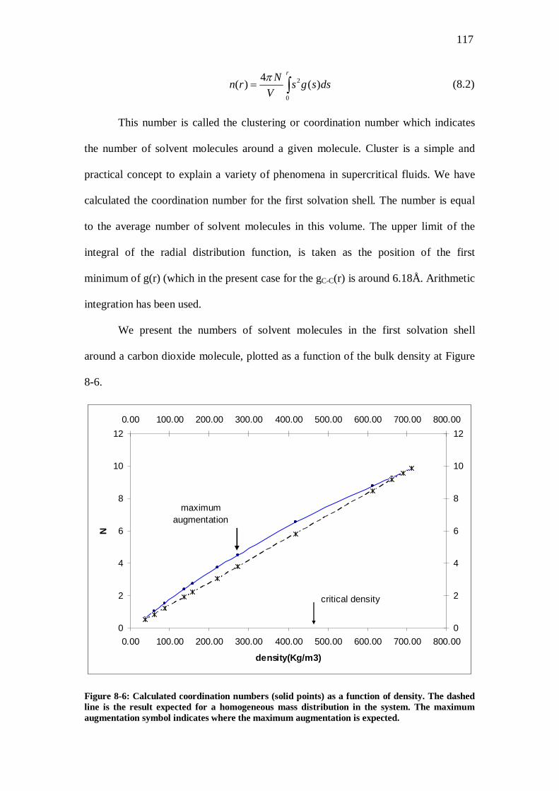
117

2

0

4( ) ( )rNn r s g s ds

V

(8.2)

This number is called the clustering or coordination number which indicates

the number of solvent molecules around a given molecule. Cluster is a simple and

practical concept to explain a variety of phenomena in supercritical fluids. We have

calculated the coordination number for the first solvation shell. The number is equal

to the average number of solvent molecules in this volume. The upper limit of the

integral of the radial distribution function, is taken as the position of the first

minimum of g(r) (which in the present case for the gC-C(r) is around 6.18Å. Arithmetic

integration has been used.

We present the numbers of solvent molecules in the first solvation shell

around a carbon dioxide molecule, plotted as a function of the bulk density at Figure

8-6.

0

2

4

6

8

10

12

0.00 100.00 200.00 300.00 400.00 500.00 600.00 700.00 800.00

density(Kg/m3)

N

0

2

4

6

8

10

120.00 100.00 200.00 300.00 400.00 500.00 600.00 700.00 800.00

critical density

maximum augmentation

Figure 8-6: Calculated coordination numbers (solid points) as a function of density. The dashed line is the result expected for a homogeneous mass distribution in the system. The maximum augmentation symbol indicates where the maximum augmentation is expected.

118

As it has been reported firstly by Tucker and co-workers (Tucker, 1999;

Tucker and Maddox, 1998) in their two dimensional SCF simulations, local density

inhomogeneities become more pronounced at lower densities to the critical density.

According to the experimental studies (Song et al., 2000), it is believed that they are

maximised at densities around (2/3)c. The local coordination number calculated from

the area underneath the first solvation shell as it is shown in the Figure 8-4 though the

equation (8.2). The enhancement is quite strong at densities close to the critical one

and lower ones. We cannot verify that it takes place at density around (2/3) c exactly.

However, our results agree with their observations. The enhancement is becoming less

pronounced at the second solvation shell, but still we can observe that there is a

difference between the bulk and the local density at Figure 8-7.

0

5

10

15

20

25

30

35

40

45

0.00 100.00 200.00 300.00 400.00 500.00 600.00 700.00 800.00

density(Kg/m3)

N

0

5

10

15

20

25

30

35

40

450.00 100.00 200.00 300.00 400.00 500.00 600.00 700.00 800.00

critical density

maximum augmentation

Figure 8-7: Coordination number at the second solvation shell. The layout and the line styles are the same as previous figure.

We believe this ‘density augmentation’ is a universal behaviour in

supercritical fluids, indicating that there is a sponge like structure in supercritical

119

phase, but as density increases the fluid looks like dense fog. It can be concluded the

sponge like structure is pronounced at densities close to critical density, which this

local structure enhancement can be seen as regions with high and low density in the

supercritical fluid.

The local structure around a molecule is definitely important factor for its

behaviour. At the moment, the lifetime of a configuration, which represents a low or a

high density structure around a molecule, is not well studied. We can realize the

importance of studying the lifetime of the local structure, when we suppose the

molecule is a reacting solute.

8.4 ISOTHERMAL COMPRESSIBILITY

Isothermal compressibility is a useful probe of long-range interactions and

their effect on the microstructure of a supercritical fluid. The isothermal

compressibility expresses the ability of the molecules in a fluid to pack more tightly,

and is the macroscopic response of a fluid to an applied pressure. The mathematical

relationship between molecular packing and can be written in terms of the radial

distribution function according to KB theory.

2

0

1 4 ( ( ) 1)B TT r g r dr

(8.3)

where B is the Boltzmann’s constant and v the density of solvent. The above

equation was introduced for a system where N may vary (grand canonical ensemble).

However Matubayasi and Levy (Matubayasi and Levy, 1996) introduced an

alternative formulation of the KB expression in the Canonical ensemble

120

2 1

2 0 0

10

0

4 ( )4 ( ( ) 1)

1 ( )

uv

uv

uv

r r drr g r dr

N r dr

(8.4)

where N is the number of solvent molecules in the system, is the bulk density of

solvent ( /v vN V ), uv is the product of the bulk density of solution and the

canonical radial distribution function. However, the authors proved that the KB theory

is valid in other ensembles and the formula in equation (8.3) can be used in the

Canonical ensemble. Others (Akiya and Savage, 2000a) used KB theory in the

Canonical ensemble by applying equation (8.3). Using the equation (8.3) we have

calculated the isothermal compressibility. The isothermal compressibility as a

function of pressure is shown in Figure 8-8.

0

0.1

0.2

0.3

0.4

0.5

0.6

0.7

0.8

4 5 6 7 8 9 10 11P(MPa)

K T(M

pa-1

)

Figure 8-8: Isothermal compressibility of CO2 T as a function of pressure at temperature T=308.15K. The pressure on axis represents the real pressure of the molecular system.

The simulation results are in good agreement with behaviour of the isothermal

compressibility in the supercritical region. However, the absolute value of the peak in

Figure 8-8 is different from the one in Figure 8-9 but lets have a better look to this.

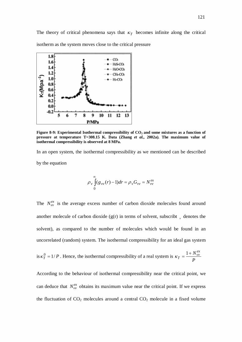
121

The theory of critical phenomena says that T becomes infinite along the critical

isotherm as the system moves close to the critical pressure K T

(Mpa

-1)

Figure 8-9: Experimental Isothermal compressibility of CO2 and some mixtures as a function of pressure at temperature T=308.15 K. Data (Zhang et al., 2002a). The maximum value of isothermal compressibility is observed at 8 MPa.

In an open system, the isothermal compressibility as we mentioned can be described

by the equation

0

)1)(( exvvvvvvvv NGdrrg

The exvvN is the average excess number of carbon dioxide molecules found around

another molecule of carbon dioxide (g(r) in terms of solvent, subscribt v denotes the

solvent), as compared to the number of molecules which would be found in an

uncorrelated (random) system. The isothermal compressibility for an ideal gas system

is PT /10 . Hence, the isothermal compressibility of a real system is PN ex

vvT

1

According to the behaviour of isothermal compressibility near the critical point, we

can deduce that exvvN obtains its maximum value near the critical point. If we express

the fluctuation of CO2 molecules around a central CO2 molecule in a fixed volume

122

away from the central one, we have NtNN )( , in which case the isothermal

compressibility can be written as

NNtN

T

)(

As T reaches its maximum near the critical point, it undergoes large fluctuations

about its average value over time. As MD trajectories through solving the Newton

equation in order to find the positions of molecules with time, they have a difficulty

following the fast movement of the molecules in “real” carbon dioxide, so they

underestimate the value of isothermal compressibility. It also has to be considered that

these density fluctuations near the critical point are correlated over a long range

(radial distribution function decays slowly) so that larger systems are required to

describe properly the molecules that are entering a fixed volume and the molecules

that are exiting it at a given distance for r in g(r). As fluctuation in local structure is

high, possibly more time consuming simulations required to improve the accuracy of

the calculated isothermal compressibilities near critical density. It is not so difficult to

imagine that this kind of inhomogeneity effects the kinetic energy distribution.

Sometimes it can cause a serious breakdown even in the constant-temperature

molecular dynamics simulation by Berendsen method.However, even with these

improvements it will be a discrepancy between real and of the predicted value because

of the nature of molecular dynamics and the nature the microscopic structure of the

real world of fluids. This fact does not reduce the incredible value of the molecular

dynamics simulations, as they mimic the physical movements of the molecules in the

compressible regime at a satisfactory level resulting in quite reliable predictions.

123

0.4

0.45

0.5

0.55

0.6

0.65

0.7

0.75

5 6 7 8 9 10 11 12 13

P (MPa)

KТ

(1/M

Pa)

Figure 8-10: MC Simulation results for Isothermal compressibility of pure CO2 at T = 308.15 K. The pressure on axis represents the real pressure of the molecular system.

The isothermal compressibility was also calculated through Monte Carlo

simulation with the same technique. Figure 8-10 shows the isothermal compressibility

versus pressure. The prediction from Monte Carlo simulation has the same

discrepancy with experimental results. Still, in this case the discrepancy can be

attributed to limitations of molecular simulations, but it proves that Monte Carlo and

molecular dynamics have the same limitations near the critical point. As Monte Carlo

and molecular dynamics give similar results, the limitation can be attributed to

potential EPM2.

8.5 DIFFUSIVITY

The diffusion coefficient in the supercritical region is one of the important

properties for the design of supercritical fluid extraction and reaction processes.

Accurate measurements are, however, very difficult especially in the critical region

where density fluctuations become large. Some experimental results have reported an

anomalous decrease of diffusion coefficients of solutes at the vicinity of the critical

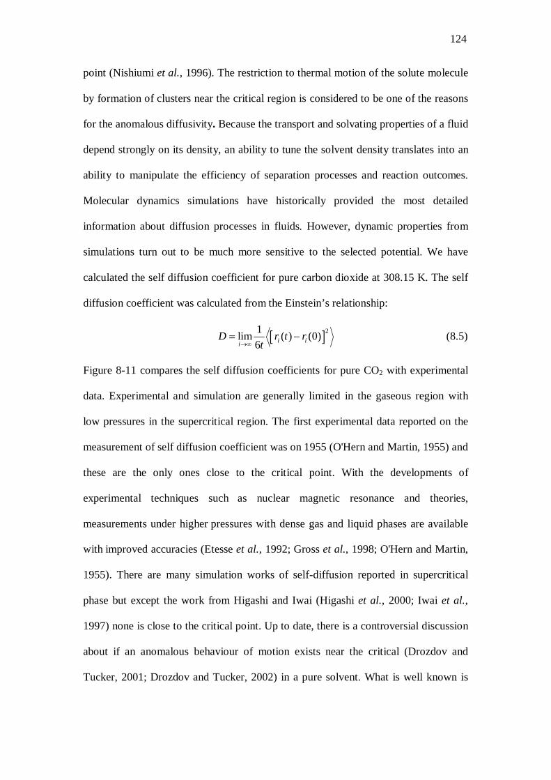
124

point (Nishiumi et al., 1996). The restriction to thermal motion of the solute molecule

by formation of clusters near the critical region is considered to be one of the reasons

for the anomalous diffusivity. Because the transport and solvating properties of a fluid

depend strongly on its density, an ability to tune the solvent density translates into an

ability to manipulate the efficiency of separation processes and reaction outcomes.

Molecular dynamics simulations have historically provided the most detailed

information about diffusion processes in fluids. However, dynamic properties from

simulations turn out to be much more sensitive to the selected potential. We have

calculated the self diffusion coefficient for pure carbon dioxide at 308.15 K. The self

diffusion coefficient was calculated from the Einstein’s relationship:

21lim ( ) (0)6 i ii

D r t rt

(8.5)

Figure 8-11 compares the self diffusion coefficients for pure CO2 with experimental

data. Experimental and simulation are generally limited in the gaseous region with

low pressures in the supercritical region. The first experimental data reported on the

measurement of self diffusion coefficient was on 1955 (O'Hern and Martin, 1955) and

these are the only ones close to the critical point. With the developments of

experimental techniques such as nuclear magnetic resonance and theories,

measurements under higher pressures with dense gas and liquid phases are available

with improved accuracies (Etesse et al., 1992; Gross et al., 1998; O'Hern and Martin,

1955). There are many simulation works of self-diffusion reported in supercritical

phase but except the work from Higashi and Iwai (Higashi et al., 2000; Iwai et al.,

1997) none is close to the critical point. Up to date, there is a controversial discussion

about if an anomalous behaviour of motion exists near the critical (Drozdov and

Tucker, 2001; Drozdov and Tucker, 2002) in a pure solvent. What is well known is

125

that the supercritical fluids exhibit large diffusion coefficients, which resemble those

of gases than those of liquids.

The diffusion coefficient in the supercritical region is strongly dependent on

temperature and pressure D=D(T, P). The temperature dependence of D in isobaric

change can be interpreted through an Arrhenius plot. Transition state theory can be

used to interpret the temperature dependence of the diffusion coefficient through the

equation )/(0)( RTE

p eDD (equivalent to Arrhenius equation). These

activation energies usually depend on pressure and density (Drozdov and Tucker,

2001). In the same way, the pressure dependence on the diffusion coefficient can be

interpreted through an equivalent equation. The slope of the diffusivity with pressure

gives the activation volume. The activation volume is defined as

ln

T const

DV R TP

(8.6)

Up to now, we really do not know how or even if, local density inhomogeneities

affect molecular diffusion coefficients, which is an important transport property

necessary for the prediction of chemical reaction rates and the design of SCF reactors.

We present the diffusion coefficient results for the critical isotherm T=1.02Tc.

The simulation results are in good agreement with experiments studies. Inspection of

Figure 8-11 shows that the diffusion coefficient of CO2 decreases with increasing

pressure. Until the pressure reaches the critical pressure, the diffusion coefficient is

quite large and resembles the one from gas phase after that, the diffusion coefficient

resembles the one from liquid phase. This fact is in a good agreement with the theory

of the two supercritical region area divided by a ridge, which the locus of the points

where the values of the density fluctuation become maximum in isothermal change

(Nakayama et al., 2000; Nishikawa and Morita, 2000). The same can be deducted

126

from the work of Gross et al (Gross et al., 1998) about their experimental results in

the supercritical region, that diffusivities on an isotherm for pressures below the one

corresponding to ridge pressures resembling those of gas phase and above the liquid

phase ones. Our simulation results agree well with this theory. In the work of Higashi

et al (Higashi et al., 2000) the carbon dioxide has been treated as united atom from

which we can concluded that an all atom representation is better than a united one for

diffusivity prediction close to the critical point.

Figure 8-11: Diffusion coefficient versus pressure at 308.2 K for pure carbon dioxide. a) Experimental data (O’Hern and Martin) b) simulation data from our work (sim) c) simulation data (Higashi et al)

On the measurements by O'Hern and Martin we can observe that there is an

increment on the self-diffusion near the critical pressure. Unfortunately, some existing

experimental results (Trappeniers and Oosting, 1966) on diffusion in SCFs are

controversial and do not clarify the situation. On the other hand, experimental

observations of the self diffusion coefficient of solutes in dilute SCF solutions

(Nishiumi et al., 1996; Nishiumi and Kubota, 2007; Tsekhans, 1971) slows down

abruptly near the liquid-gas critical point of these solute-solvent systems. However,

127

our conventional molecular dynamic studies have not revealed any anomaly close to

the critical point.

8.6 ISOCHORIC HEAT CAPACITY

The constant volume heat capacity, VC can be calculated from the fluctuations

in potential energy from MC or MD simulations by

22

2O

V VB

E EC C

k T

(8.7)

where 22 EE the potential energy fluctuation, kB is the Boltzmann constant, and

T is the absolute temperature. OVC is the ideal gas heat capacity contribution. In case of

a polyatomic gas like CO2 the ideal partition function is a product of electronic,

nuclear, rotational, translational and vibrational partition functions. According to the

procedure being followed in every statistical mechanic text (Van P.Carey, 1999), the

formulation gives the ideal part of heat capacity for a polyatomic gas as

2 /3 6

/ 21

3 32 2 ( 1)

j

j

Tnj

V Tj

eC RT e

(8.8)

The first term comes from the translational contribution to the heat capacity, the

second term is the rotational contribution and the last term is due to the vibrational

degrees of freedom. In the case of carbon dioxide, the rotational contribution is 2/2

since it is a linear molecule. The calculation of ideal heat capacity through statistical

mechanics is accurate near the critical temperature, as we can see from Figure 8-12.

In Figure 8-13, we present the simulated heat capacity in comparison to the

experimental data and values from Wagner’s equation of state. The simulated results

are in good agreement, considering the difficulties performing simulations in

128

supercritical phase and the fact that the heat capacity is calculated as the second

derivative of energy.

25

30

35

40

45

50

200 300 400 500 600 700 800 900 1000

T (K)

Cv

(J/m

ol K

)C

v(kJ

/mol

K)

Figure 8-12 . Ideal heat capacity ().Experimental Values from NIST database () Theoretical Values

0

10

20

30

40

50

60

70

0 2 4 6 8 10 12P(MPa)

C V(K

J/m

ol)

0

10

20

30

40

50

60

700 2 4 6 8 10 12

Cvlit Cvsim CvNIST

Figure 8-13: Dependence of VC on pressure for pure CO2.a) Cvlit data (Zhang et al., 2002c) b) data from Molecular Dynamics simulation c) data from NIST database

129

It is of great importance that the value of VC has its maximum close to the

critical pressure as we can conclude that the molecular potential we used predict and

describes the supercritical region properly; even at temperatures very close to the

critical point. The large fluctuations and formation of clusters in the neighbourhood of

the critical point therefore result in an abnormally large specific heat capacity. The

finite value of isochoric heat capacity near the critical point is a property depending

on the number of clusters; in other words, the size and the number of high density and

low density regions in the solvent. In order to realize better the concept of a cluster,

we should have in mind that is a dynamic process, which has breaking and formation

time. The peculiar nature of the supercritical phase, with rapid formation and

breakdown of clusters and the rapidly increased number of cluster is the reason for

maximizing the value of the isochoric capacity. The discrepancy between the

experimental value and the simulated one is because of the limits of molecular

simulations as we discussed for isothermal compressibility.

130

9 SOLUTION PROPERTIES OF MIXTURES AT

INFINITE DILUTION

t has been one of the important subjects in supercritical research to understand

how the solvent influences chemical reactions. There have been many

experiments to investigate the solvent effects on the chemical reactions.

Numerous phenomenological data are available on examining the solution effect on

reacting solutes, but no universal theory exists to interpret them. The experimental

approaches are undoubtedly a powerful tool for the investigation of the solvent effects

on chemical reactions, but a strong theory needs to be established to expand the use of

supercritical carbon dioxide in industry.

In this chapter, we look deeply into the solvent effect on the solute. The goal

of this work is to establish a relation between the degree of aggregation or cavitation

and thermodynamic properties, such as diffusivity, heat capacity and partial molar

volumes of the solute. Once more, the Kirkwood and Buff fluctuation theory, which is

describing non-ideal solutions including supercritical solutions, is used to evaluate the

micro-environment of the solutions. The objective is to examine the tendency of the

solvent to form clusters or cavitations across different kind of solutes regarding the

pressure dependence along a critical isotherm.

I

131

9.1 INTRODUCTION

The role of local density in influencing chemistry in supercritical fluids is a

key element to our understanding of reaction dynamics. At temperatures appreciably

higher than the critical temperature T>Tc, the solvent fluid itself is rather uniform and

homogeneous and the isothermal compressibility of the fluid is not large. However,

when for example a solute with large attractive solute-solvent interactions is placed in

the fluid, the solvent molecules form a cluster surrounding the solute molecule. The

number of solvent molecules participating in the cluster under such conditions is

rather small and they form only the first solvation shells, in contrast to large clusters

near the critical point

In traditional solution thermodynamics, the process of solvation can be

thought of two steps, finding space and occupying it. In previous chapter, we have

seen the random movements of the molecules cause cavities (void spaces in the fluid)

to form. The likelihood of a cavity being available to a solute particle is proportional

to the density of the fluid; dense systems have few large cavities. According to

conventional theories of solution, somebody expects the cavity must be sufficiently

sized and shaped to allow a solute particle to move into the cavity during solvation

process. The size of cavities is maximized close to the critical point. One expects that

the size of cavitations should pass through a maximum with increasing pressure on a

critical isotherm.

9.2 INFINITE DILUTION OF METHANE IN SUPERCRITICAL

CARBON DIOXIDE

Experimental observations (Zhang et al., 2002a) found that the addition of

methane into supercritical carbon dioxide increases the volume of solution. Their

132

group reported large positive partial molar volumes near the critical pressure, which is

evidence that the system volume increases. While the partial molar volume is a

macroscopic thermodynamic property, their measurements could be interpreted to

show the cavitation of carbon dioxide molecules around methane molecule.

A system, consisting of 999 carbon dioxide molecules and 1 molecule of

methane, is used to represent the infinite dilution of methane in the supercritical

carbon dioxide. As the addition of one methane molecule into 999 molecules gives a

mixture 0,1% per volume, we assume that the critical point of the mixture remains the

same. The correlation functions were determined by using the centre of each species,

the carbon atom. We sampled the radial distribution function every 1000

configurations during MD simulations

A sampling diagram from the radial distribution functions for Tr = 308.15 K

over the densities ranging from 135.79 kg/m3 to 712.3 kg/m3 (critical density of CO2

is 468 kg/m3) for CO2-CH4 is shown in the Figure 9-1. The choppy appearance of the

solute-solvent radial distribution function is common and has been observed in other

infinite dilute solute mixtures simulations (Akiya and Savage, 2000b). The Figure 9-1

shows that the radial distributions functions exhibit a clear difference in appearance at

subcritical and supercritical densities. The peak height decreases with increasing

density from subcritical to supercritical ones and a second shell appears which is in

agreement with theory (Clifford, 1999). Figure 9-2 shows the solute-solvent and

solvent-solvent radial distribution functions for CO2-CH4 and CO2-CO2 pairs.

Comparing the Figure 9-1 and Figure 8-4, we can see the trend of the RDF for

carbon dioxide is strongly dependent on carbon dioxide bulk density compared to

carbon dioxide-methane interaction. The height of the peaks and the contrasting

133

trends demonstrate that the strength of methane-carbon dioxide interactions relative to

carbon dioxide-carbon dioxide interactions are lower.

0

0.2

0.4

0.6

0.8

1

1.2

1.4

1.6

0 5 10 15 20 25 30 35 40

r (Angstrom)

g(r)

ρ = 135.96 kg/m3ρ = 243.98 kg/m3ρ = 769.30 kg/m3

= 135.79 kg/m3 r= 220.72 kg/m3r= 712.30 kg/m3

Figure 9-1: Pair correlation function for mixture of CH4-CO2 at different densities

0

0.2

0.4

0.6

0.8

1

1.2

1.4

1.6

1.8

2

0 10 20 30 40 50 60r (Angstrom)

g(r)

SS Ss

Figure 9-2: Comparison of pair correlation function obtained for pure CO2 (SS) and mixture of CO2-CH4 (Ss) at T = 308.15 K and density equal to 272.79 kg/m3.

134

When we compare the RDFs of solute-solvent and solvent-solvent in the same

graph (Figure 9-2) it is obvious that the number, exN which gives the amount of excess

molecules around a solute molecule, is negative.

( )oex v uv vvN G G (9.1)

As in our discussion in the previous chapter, we will use the shape of the

radial distribution function to interpret the results. The clustering number has been

estimated by integrating the radial distribution function within an appropriate range, r1

to r2 which defines the solvation shell. It is given by the following equation

2

212

1

4 ( )r

clusr

N g r r dr (9.2)

In our case, the g12 is the radial distribution function between the carbon atom of CH4

and the one from carbon dioxide. The value of r1 is equal to zero and the value of r 2 is

equal to the distance where the first minimum in g(r) is being observed. In this case

the upper bound for the integral in our highest densities results, the position of the

minimum is around 6.68 Å. Actually, the value of r1 is not equal to zero. The value of

r1 it depends on the size of the molecule and it the closest distance which two

molecules can approach each other. The values r1-r2 in the integration for the

calculation of the number of clustering around a methane molecule are different from

the values used into the integration around a carbon dioxide molecule. So a directly

comparison of the two coordination number can not be made, but a comparison with

the coordination number in case that expected when we had a homogeneous fluid can

be made.

The isothermal compressibility expresses the gathering of an enormous

number of solvent molecules. The range of gathering molecules is quite long, and

becomes maximum for c. The infinite value of the isothermal compressibility near

135

the critical point can be classified as a long-range phenomenon. On the other hand,

depletion or clustering ordinary indicates the gathering of the solvent molecules of a

few angstroms and can be classified as a short-range phenomenon.

We present in Figure 9-3 the coordination number of CO2 molecules around a

CH4 molecule in a homogeneous fluid at same density and the coordination number of

CO2 molecules around a CH4 molecule in the real fluid. Comparing the Figure 9-3 and

Figure 8-6 we can more clearly understand now that the Nex it is a negative number,

which means that there is a depletion of CO2 molecules around the methane, in other

words a cavitation exists around the methane molecule. From the two figures, we can

deduce that the maximum depletion occurs at densities below the critical one. The

higher cavitation around a methane molecule occurs at densities where the maximum

local clustering has been observed for the pure carbon dioxide. So, the depletion or

the clustering is the kind of process occurs in short range around a solute and belongs

to short range phenomena. In other words the addition of a solute molecule in a

supercritical fluid in change the microstructure of the supercritical fluid only in a short

distance around it, it cannot change dramatically the whole microstructure of the

supercritical fluid.

Our observation that the addition of methane molecules into the supercritical

carbon dioxide cause depletion around it, agrees well with experiments. The depletion

around the methane molecule, leads to expand the volume of solution of the whole

mixture. This agrees well with experimental studies as Zhang et al reported positive

partial molar volumes of the dilution of methane into supercritical carbon dioxide.

However, the solute partial molar volume is a quantity, which maximised at

the point, where the isothermal compressibility obtains its maximum value on a

critical isotherm. This means that the partial molar volume at supercritical solutions is

136

a property is connected more with behaviour of bulk density rather than the local

density.

0

2

4

6

8

10

12

14

16

0.00 100.00 200.00 300.00 400.00 500.00 600.00 700.00 800.00

density(Kg/m3)

N

0

2

4

6

8

10

12

14

160.00 100.00 200.00 300.00 400.00 500.00 600.00 700.00 800.00

Figure 9-3: Coordination number of CO2 molecules around a methane molecule` (solid line) and coordination number (dashed line) of a homogeneous fluid at same density.

In addition, combining the equations (9.1) and (4.7) we can extract a formula

connecting the excess or depleted number of molecules around a solute, with the

solute partial molar volume at infinite dilution. We obtain:

ex

uNV

1

According to this formula if we calculate the solute partial molar volume in the first

solvation shell it will appears to go through a maximum near (2/3)c. However, the

solute partial volume diverges close to critical density along an isotherm. Based on

the fact we can conclude partial molar volume is a macroscopic property, which

reflects more the nature of the solvent rather than the nature of local interactions.

137

The formation of cavitations around repulsive solutes is an interesting process

but to the best of our knowledge, there is no industrial application using this feature.

We believe this kind of solvent can used as co-solvents in order to expand the

common features (clustering) of supercritical fluids. All the supercritical solutions in

technological applications are cases of attractive clustering mixtures e.g.,

decaffeination of coffee and other examples of supercritical fluid extraction,

supercritical chromatography, sorbent regeneration by supercritical fluids. These

mixtures are characterised by large negative solute partial molar volumes near the

solvent critical point. The mixture of water and supercritical carbon dioxide belongs

to that category. We will examine that system in the next section.

9.3 INFINITE DILUTION OF WATER IN SUPERCRITICAL

CARBON DIOXIDE

The research group of (Zhang et al., 2002a) reported negative partial molar

volumes of water and carbon dioxide at infinite dilution. We followed exactly the

same approach as in the case of methane with carbon dioxide, in order to examine the

microstructure of the solution. We present the coordination number of CO2 around a

water molecule in Figure 9-4. There is an enhancement of local density around the

water molecule. The degree of density enhancement is stronger than those of a CO2

molecule. According to experimental studies (Song et al., 2000) the larger degree of

clustering appears at densities below the critical one. Figure 9-4 shows the maximum

clustering occurs at densities around 300 kg/m3. Our simulation results are in line with

experimental observations and we can verify that the maximum degree of clustering

occurs at densities around (2/3)c for an attractive solute.

138

0

2

4

6

8

10

12

0.00 100.00 200.00 300.00 400.00 500.00 600.00 700.00 800.00

density(Kg/m3)

N

0

2

4

6

8

10

120.00 100.00 200.00 300.00 400.00 500.00 600.00 700.00 800.00

critical density

maximum augmentation

Figure 9-4: Coordination number of CO2 molecules around a water molecule` (solid line) and coordination number (dashed line) of a homogeneous fluid at same density

9.4 THERMODYNAMIC PROPERTIES OF MIXTURES AT

INFINITE DILUTION

9.4.1 Diffusivity We calculated diffusion coefficients of one methane molecule in supercritical

carbon dioxide (repulsive mixture) and one water molecule in supercritical carbon

dioxide (attractive mixture). The results are being presented in Figure 9-5. The tracer

diffusion coefficient for both methane and water goes abruptly to zero close to the

critical point. The reason is to investigate characteristics of the cluster structure

around the water molecule and the cavitation structure around the methane molecule.

We used the normal Einstein’s relation to estimate the diffusion coefficient D. Up to

date there two concepts used to explain the reason for the drastic change of the

diffusion coefficient near the critical pressure along an isotherm. One is the change in

effective mass of the cluster caused by solvent molecules around the solute molecule,

139

and another is the density fluctuation of the solvent fluid where the solute molecules

move. We believe that the first concept is most likely not the origin of the anomalous

decrease of diffusivity near the critical point. There are two facts that disagree with

this concept. Firstly, if the clustering would have a restrictive role on the solute

movement, the diffusivity would be expected to have an anomalous behaviour at

densities where the maximum local density enhancement has been observed.

Secondly, a repulsive mixture should not exhibit an decrease in diffusivity but rather

an increase as the solute molecule is in the middle of a cavitation and has a lot of

room to move. In other words it is not the clustering, which forbids the solute from

moving. The anomalous diffusivity has been observed for an attractive solute at

infinite solution at density close to the critical one as well as a repulsive solute. This

phenomenon has been observed for both systems in the region of the phase diagram,

which is characterised by spatially extended fluctuations in the fluid density. We

believe the extent of these fluctuations is related to the anomalous solute diffusion

coefficient for both, the attractive and the repulsive solute.

In order to understand the anomalous diffusivity, it is necessary to realize the

nature of the microenvironment around the solute. Furthermore, it is necessary to

understand beyond the description provided by the radial distribution function around

the solute, as this indicator describes only the average of all the environments found

within the fluid. For an attractive solute, the distribution of microstructures containing

the solute is changing rapidly over the time near the critical point. The same is

happening for a repulsive solute too. The rapid rearrangement of the microstructure

around the solute does not give free space for the solute to move. The instantaneous

environment around the solute in a short range changes so dramatically with time, that

140

the free positions for an attractive solute or a repulsive one are always engaged

restricting the motion of the solute molecule.

-100

400

900

1400

1900

0.00 2.00 4.00 6.00 8.00 10.00 12.00P(MPa)

DC

O2 x109 [m

2 /sec

]

-100

400

900

1400

1900

0.00 2.00 4.00 6.00 8.00 10.00 12.00

D(CO2) D(H2O-CO2) D(CH4-CO2)

Figure 9-5: Dependence of tracer diffusion coefficient on pressure of i) a CO2 molecule in pure CO2 ii) a CH4 molecule in CO2 and iii)a H2O molecule in CO2 .Solutions 0.1mol% and temperature 308.15K.

Moreover, our explanation is in agreement with the kinetic theory of gases.

The molecules in a gas move with quite high speeds. If a little ammonia gas is

released at one end of a room, however, an appreciable time elapses before the smell

is noticed at the opposite end. The reason for the slowness is that the molecules are

constantly entering into collisions, so that the long path, which a single molecule

would describe if it were unimpeded, is broken up into a very large number of zigs-

zags in all directions. Since, the mobility of solvent molecules is maximed near the

critical point; the solute molecule is constantly deflected by collisions with solvent

molecules, so the free path is very short. Its position is nearly stationary resulting in

zero diffusion coefficients.

9.4.2 Isochoric Heat Capacity Constant volume heat capacity (CV) is directly related with internal energy,

and thus can provide information about the intermolecular interaction in the system.

141

CV of a mixed fluid depends mainly on its composition and intermolecular

interactions. At a fixed composition, CV should depend mainly on the intermolecular

interaction. CV has a weak divergence at the critical point, which implies that is

connected with the first and second solvation shell (radial distribution function)

instead of the tail, as it is the case with isothermal compressibility. In other words

these means that the isochoric heat capacity is related to structure of the molecules in

short distance around it compare to molecules at long distance.

Furthermore, CV of pure components or mixtures is nearly independent of

pressure in high pressure region, indicating that the intermolecular interaction is not

sensitive to pressure as the fluid is far from the critical region of the mixed fluids. In

the critical region, the Cv depends on pressure and is sensitive to composition because

of the nature of the supercritical phase.

20

25

30

35

40

45

50

0 2 4 6 8 10 12P(MPa)

Cv(K

J/m

ol)

20

25

30

35

40

45

500 2 4 6 8 10 12

Cv(CO2-H2O) Cv (CO2-CH4) Cv CO2

Figure 9-6Dependence of Cv on pressure for pure CO2, CH4-CO2 and H2O-CO2 systems (0.1mol% mol) at 308.15K

Cv(

kJ/m

ol)

142

The first peak of the radial distribution function represents a statistical average

of the neighbours around a chosen molecule. As we have explained in the section 8.4,

the observed structure around a central molecule, it fluctuates with the time. In the

case of methane and carbon dioxide, we have a depletion (lack of molecules) around

the methane molecule. In the case of water and carbon dioxide mixture we have an

enhancement (excess of molecules) around the water molecule. The way the

microenvironment changes around a solute molecule with time become faster when

isothermal compressibility obtains its maximum value. We believe that the larger rate,

i.e. the speed the molecules come into and leave the tagged area around a solute in the

high compressible regime is the reason for the maxima in the curves. An increase in

temperature results in decrease in the degree of clustering. Some of the members in

the clusters enter into the bulk, which needs some additional energy. Therefore, the

largest Cv indicates higher clustering. On the basis of this discussion, it can be

deducted that breaking the clusters at the supercritical conditions is an endothermic

process. The cluster formed around a water molecule is strongly holding together

(strong attractive forces between the solute molecule and solvent molecules) which is

more difficult to break than a pure CO2 cluster. On the other hand, the cluster around

the methane molecule is a weak one (weak attractive forces) and can be easier broken

than pure CO2. This fact explains why the solution of water in supercritical carbon

dioxide increases the heat capacity while the solution of methane decreases it.

143

10 CONCLUSION AND FUTURE WORK

n this work, we have successfully employed molecular simulation methods

using the potential model EPM2 to derive different thermodynamic properties

of pure carbon dioxide, a mixture of methane-carbon dioxide and a mixture of

water-carbon dioxide at infinite solution. The transferability of EPM2 model to the

supercritical region has been studied through a comprehensive comparison between

calculated values of several thermodynamic properties for CO2 and experimental

values.

Molecular simulation, although having plenty of room for improvement, can

be reliably used to study difficult systems like supercritical fluids where experimental

observations are problematic. Moreover, they provide an insight to the systems on

atomic scale which enables us to establish a relationship between intermolecular

potential and thermodynamic properties. In our study however, we identified a

problem of MC being unable to predict realistic property values in the low density

region. The reason for this is the trapping of MC sampling in unphysical

configurations.

Beyond pure supercritical fluids, supercritical mixtures at infinite dilution can

be studied with the existence of valid molecular force fields. We also observed some

deviations in the results of isothermal compressibility and heat capacity from

experimental data. These deviations however were due to computational limitations

rather than the employed methodology.

Beside the usefulness of molecular simulation in predicting fluid properties in

the supercritical region, it gives an insight in events at microscopic level with time

and space. It enables us to calculate numerically the radial distribution function which

I

144

we used to examine the microstructure of supercritical conditions with regard to local

structure using the KB theory

In the application of the KB theory to the systems

1. Pure carbon dioxide

2. Infinite dilution of methane in carbon dioxide

3. Infinite dilution of water in carbon dioxide

We identify three types of local microstructure.

Type A. There is local density enhancement of CO2 around a CO2 molecule.

This density enhancement is more pronounced at densities below the critical one (ca.

2/3ρc). In other words there is a sponge like structure of CO2 molecules in

supercritical region which is more evident at densities below the critical density along

an isotherm. Type B. There is also a density enhancement around a water molecule in

CO2 molecules. This has been identified as an excess of CO2 molecules around a

water molecule. Rephrasing, the water molecule prefers to solvate in high density

region of carbon dioxide. Type C. There is a density depletion of CO2 molecules

around a methane molecule. In this situation, this has been identified as a deficit of

CO2 molecules around a methane molecule. In other words, the water molecule

prefers to solvate in areas where there is cavitation.

An apparently counter-intuitive point in the three different pictures of

solvation is that they follow the same trend. They show the most anomalous

behaviour at the same densities along the critical isotherm. Two unrelated solutes,

when being dissolved in supercritical carbon dioxide, follow somehow a ‘universal’

behaviour, despite the fact that they follow a different type of solvation. This

universal behaviour is related more to the properties of the supercritical carbon

dioxide rather than the properties of the individual solutes, water or methane. In other

145

words the structure of carbon dioxide is very important in any solvation at

supercritical conditions. The density augmentation or depletion is not caused by the

solute, but rather it is due to the pre-existing densities inhomogenities in the pure

solvent. The solute only shows a preference to dissolve in a high density region or low

density region.

Furthermore, this apparently ‘universal’ behaviour is observed also for

diffusion coefficients. The diffusion coefficient of methane in the supercritical carbon

dioxide drops abruptly to zero, the same as in the case of water. Furthermore, this

drop happens around the same density. We noted that the density where this is

observed coincides with that where fluctuations in local density obtain their maximum

value. We suggest that the rapid movement of CO2 around a solute molecule is the

driving force for zero values of diffusion coefficients. The rapid movement of solvent

molecules around a solute restricts the motion of the solute and gives zero values of

solute diffusion coefficients.

It can be concluded that the nature of the solvent is crucial in any observed

pure or solvation property. This nature is yet not well understood and is still a matter

of debate. We believe the preference of the solute to move in a high density region or

low density region and the high density fluctuations near the critical point are most

likely responsible for any peculiarities in pure or solvation properties. To date little

work has been done about the instantaneous environment of a solute molecule in a

supercritical fluid. This will help us to understand a second key characteristic of

supercritical nature not their fluctuation in space but their fluctuation with time. This

is an important factor for reaction dynamics in solvent-influenced chemical reactions.

At the present time, the principal source of information on the instantaneous structure

146

is computer simulations. We believe an important aspect that has to be studied along a

supercritical isotherm with pressure is the size a cavitations or clusters with time.

On the basis of our study, one can now imagine a general mechanism of a

solution chemical reaction from a microscopic point of view. The solution-chemical

reaction is viewed as a passage of a solute molecule over the solute potential-energy

barrier, accompanied by solvent influence. The solvent, in general, play three distinct

roles.

First, some solvent molecules themselves become involved in the

rearrangement of molecules around the solute providing clustering or depletion

environment. In turn, they can modify the solute electronic state through electrostatic,

exchange, polarization, and dispersion interactions and deform the solute potential-

energy surface. Such a modification should influence the potential-energy barrier

itself along the reaction coordinate but also the properties of transition state. Second,

the interaction energy between the solute and solvent molecules sometimes induces a

considerable configurational change of the solute molecule and results in another

stabler configuration by reflecting the energetic balance between the solute potential

and the solute-solvent interaction energy as we have seen for cases of isothermal heat

capacity. Third, the reaction energy required to surmount the potential-energy barrier

should be supplied from the surrounding solvent molecules through the solvent energy

fluctuation. The solvent-solvent and the solute-solvent interactions should play such

roles as the energy source of supply.

We can conclude that new parameters have to be introduced to describe the

structure of supercritical phase. The local pressure around a solute with time is one of

them, it will help us to explain many reaction phenomena. Alternatively, we have to

realize that there is local-bulk anisotropy in pressure which is an important key in any

147

micro-kinetic analysis, especially at supercritical fluid/solid interfaces, kinetics of

adsorption. Furthermore, by defining local pressure we will understand better

transition state kinetics and will choose the proper solvation environment in a solvent

phase or microporous environment.

Another future research direction is the possibility that reactant-reactant

(solute-solute) clustering can occur that in turn will affect reaction kinetics. KB theory

with some corrections might still be used for such treatments. We believe this work of

fundamental nature will help understand the performance of supercritical fluids as

reactions media.

148

11 APPENDIX

This is program selected at random. It is describing the initialization the equilibration process

!---------------- PROGRAM BOX !---------------- ! . Module declarations. USE DYNAMO IMPLICIT NONE ! . Program parameters. INTEGER, PARAMETER :: NCHANGES = 10 REAL ( KIND = DP ), PARAMETER :: BIGSIZE = 10.0_DP ! . Thermodynamic conditions (NVT) REAL ( KIND = DP ), PARAMETER :: DENSITY = 973.1_DP !kg m^-3. ! . Monte Carlo Simulation Options REAL ( KIND = DP ), PARAMETER :: P = 14.4_DP/0.101325_DP !atm REAL ( KIND = DP ), PARAMETER :: T = 310.00_DP !kelvin REAL ( KIND = DP ), PARAMETER :: ACC = 0.40_DP !dimensionless INTEGER , PARAMETER :: NVT=0 !NVT simulation INTEGER , PARAMETER :: NPT=500 !NPT simulation ! . Program scalars. INTEGER :: ICHANGE REAL ( KIND = DP ) :: NEWSIDE, REDUCE, SIDE, TARGET, VOLUME ! . Program arrays. REAL ( KIND = DP ), ALLOCATABLE, DIMENSION(:,:) :: COORDINATES ! . Output File open(6,file="results/box=(1000 , 49.68 , 310.00).out") CALL DYNAMO_HEADER CALL TIME_PRINT CALL ZMATRIX_DEFINE ( "../data/zmatrix/CF3.zmatrix" ) CALL ZMATRIX_BUILD CALL COORDINATES_WRITE ALLOCATE ( COORDINATES(1:3,1:NATOMS) ) ; COORDINATES = ATMCRD CALL MM_FILE_PROCESS ( "solvent.opls_bin", "../data/opls_aa/solvent.opls" ) CALL MM_SYSTEM_CONSTRUCT ( "solvent.opls_bin", "../data/seq/CF3_box1000.seq" ) CALL MM_SYSTEM_WRITE ( "../data/sys_bin/CO2_CF3box1000.sys_bin" ) ! . Calculate the volume of a box that gives the appropriate density (Angstroms^3). VOLUME = ( SUM ( ATMMAS(1:NATOMS) ) / DENSITY ) * ( AMU_TO_KG * 1.0E+30_DP ) ! . Calculate the dimension of a cubic box of the same volume (Angstroms). TARGET = EXP ( LOG ( VOLUME ) / 3.0_DP ) ! . Start off with a very large box.

149

SIDE = BIGSIZE * TARGET ! . Calculate the reduction factor. REDUCE = EXP ( - LOG ( BIGSIZE ) / REAL ( NCHANGES, DP ) ) ! . Assign a value to the box size. CALL SYMMETRY_CUBIC_BOX ( SIDE ) ! . Generate coordinates for each molecule. CALL SET_INITIAL_COORDINATES ! . Initialize the random number seed. CALL RANDOM_INITIALIZE (314159) ! . Define the options for the Monte Carlo modules. CALL MONTE_CARLO_ENERGY_OPTIONS ( CUTOFF = 0.45_DP*TARGET, SMOOTH = 0.0_DP ) ! . Do a Monte Carlo simulation (at constant volume). CALL MONTE_CARLO ( 10, 10 * NRESID, VOLUME_FREQUENCY = NVT ,PRESSURE=P,TEMPERATURE=T) ! . Gradually reduce the size of the box to the desired value. DO ICHANGE = 1,NCHANGES ! . Calculate and set the new box length. NEWSIDE = REDUCE * SIDE CALL SYMMETRY_CUBIC_BOX ( NEWSIDE ) ! . Scale the coordinates. CALL SET_INTERMEDIATE_COORDINATES ! . Do a Monte Carlo simulation (at constant volume). CALL MONTE_CARLO ( 10, 10 * NRESID, VOLUME_FREQUENCY = NVT ,PRESSURE=P,TEMPERATURE=T) ! . Reset SIDE. SIDE = NEWSIDE END DO ! . Save ccordinates CALL COORDINATES_WRITE ( "../data/box(CF3)/NVT=(1000 , 973.1 , 310.00)(0).crd" ) CALL PDB_WRITE ( "../data/box(CF3)/NVT=(1000 , 973.1 , 310.00)(0).pdb" ) ! . Do a final MC calculation for a fuller equilibration. CALL MONTE_CARLO ( 200, 100000, PRESSURE=P,TEMPERATURE=T, ACCEPTANCE=ACC, VOLUME_FREQUENCY = NVT) ! . Save the coordinates CALL COORDINATES_WRITE ( "../data/box(CF3)/NVT=(1000 , 973.1 , 310.00)(1).crd" ) CALL PDB_WRITE ( "../data/box(CF3)/NVT=(1000 , 973.1 , 310.00)(1).pdb" ) ! . Deallocate the temporary arrays. DEALLOCATE ( COORDINATES ) ! . Finish up. CALL TIME_PRINT !=============================================================================== CONTAINS !===============================================================================

150

!--------------------------------- SUBROUTINE SET_INITIAL_COORDINATES !--------------------------------- ! . Local scalars. INTEGER :: I, START, STOP ! . Loop over the residues. DO I = 1,NRESID ! . Set the initial values of the coordinates. START = RESIND(I)+1 STOP = RESIND(I+1) ATMCRD(1:3,START:STOP) = COORDINATES ! . Randomly translate the molecule within the box. CALL TRANSLATE ( ATMCRD(1:3,START:STOP), SIDE * ( RANDOM_VECTOR ( 3 ) - 0.5_DP ) ) END DO END SUBROUTINE SET_INITIAL_COORDINATES !-------------------------------------- SUBROUTINE SET_INTERMEDIATE_COORDINATES !-------------------------------------- ! . Local scalars. INTEGER :: I, START, STOP REAL ( KIND = DP ) :: SCALE ! . Local arrays. REAL ( KIND = DP ), DIMENSION(1:3) :: DR ! . Calculate the scale factor for changing the coordinates of the molecular centers. SCALE = NEWSIDE / SIDE ! . Translate the coordinates of the atoms in each molecule. DO I = 1,NRESID ! . Find the atom indices for the molecule. START = RESIND(I)+1 STOP = RESIND(I+1) ! . Find the translation. DR = ( SCALE - 1.0_DP ) * CENTER ( ATMCRD(1:3,START:STOP), ATMMAS(START:STOP) ) ! . Translate the molecule by the required amount. CALL TRANSLATE ( ATMCRD(1:3,START:STOP), DR ) END DO END SUBROUTINE SET_INTERMEDIATE_COORDINATES END PROGRAM BOX

151

DL POLY : Control file SCO2 at T=308.15 and P=7.5 MPa integration leapfrog verlet temperature 308.15 pressure 0.075 ensemble nvt berendsen 0.5 steps 1000000 equilibration 500000 multiple step 4 scale 10 # collect print 1000 stack 1000 stats 1000 trajectory 500000 500 0 rdf 100 timestep 0.002 primary cutoff 25.8 cutoff 29.0 delr width 1.2000 rvdw cutoff 29.0 reaction field eps constant 78.000 cap forces 1000. #shake tolerance 1.0E-3 quaternion tolerance 1.0E-5 zdensity print rdf job time 540000 close time 6600 finish

152

12 REFERENCES

Literature Cited Akiya, N., and P. E. Savage. 2000a. Effect of Water Density on Hydrogen Peroxide

Dissociation in Supercritical Water. 1. Reaction Equilibrium. J. Phys. Chem. A 104:4433-4440.

Akiya, N., and P. E. Savage. 2000b. Effect of Water Density on Hydrogen Peroxide Dissociation in Supercritical Water. 2. Reaction Kinetics. J. Phys. Chem. A 104:4441-4448.

Allen, M. P., and D. J. Tildsley. 1989. Computer simulation of liquids. Oxford University Press, Oxford.

Andrews, T. 1869. Philos. Trans.4:226

Arrhenius, S. A. 1889. Z. Phy. Chem.159:575

Asano, T., and J. Lenoble. 1978. Activation and Reaction Volumes in Solution. Chem. Rev. 78:407-489.

Atkins, P. W. 1994. Physical Chemistry. Oxford University Press, Oxford.

Baiker, A. 1999. Supercritical fluids in heterogeneous catalysis. Chem. Rev. 99:453-473.

Berendsen, H. J. C., J. R. Grigera, and T. P. Straatsma. 1987. The missing term in effective pair potentials. J. Phys. Chem. 91:6269-6271.

Blinder, S. M. 1969. Advanced physical chemistry : a survey of modern theoretical principles. Collier-Macmillan, London.

Born, M., and R. Oppenheimer. 1927. Ann. Physik 84:457.

Brennecke, J. F., and J. E. Chateauneuf. 1999. Homogeneous Organic Reactions as Mechanistic Probes in Supercritical Fluids. Chem. Rev. 99:433-452.

Chitra, R., and P. E. Smith. 2001a. A comparison of the properties of 2,2,2-trifluoroethanol and 2,2,2-trifluoroethanol/water mixtures using different force fields. The Journal of Chemical Physics 115:5521-5530.

Chitra, R., and P. E. Smith. 2001b. Properties of 2,2,2-trifluoroethanol and water mixtures. The Journal of Chemical Physics 114:426-435.

Clifford, T. 1999. Fundamentals of Supercritical Fluids. Oxford Science Publications, Oxford.

Colina, C. M., C. G. Olivera-Fuentes, F. R. Siperstein, M. Lisal, and K. E. Gubbins. 2003. Thermal properties of supercritical carbon dioxide by Monte Carlo simulations. Molecular Simulation 29:405-412.

153

de Pablo, J. J., J. M. Prausnitz, H. J. Strauch, and P. T. Cummings. 1990. Molecular simulation of water along the liquid--vapor coexistence curve from 25 oC to the critical point. The Journal of Chemical Physics 93:7355-7359.

Debenedetti, P. G., and R. S. Mohamed. 1989. Attractive, weakly attractive, and repulsive near-critical systems. The Journal of Chemical Physics 90:4528-4536.

Drljaca, A., C. D. Hubbard, R. van Eldik, T. Asano, M. V. Basilevsky, and W. J. le Noble. 1998. Activation and reaction volumes in solution. 3. Chem. Rev. 98:2167-2289.

Drozdov, A. N., and S. C. Tucker. 2001. Self-diffusion near the liquid-vapor critical point. The Journal of Chemical Physics 114:4912-4917.

Drozdov, A. N., and S. C. Tucker. 2002. Response to ``Comment on `Self-diffusion near the liquid-vapor critical point' ''. The Journal of Chemical Physics 116:6381-6382.

Eckert, C. A., D. H. Ziger, K. P. Johnston, and S. Kim. 1986. Solute partial molal volumes in supercritical fluids. J. Phys. Chem. 90:2738-2746.

Errington, J. R., K. Kiyohara, K. E. Gubbins, and A. Z. Panagiotopoulos. 1998. Monte Carlo simulation of high-pressure phase equilibria in aqueous systems

41. Fluid Phase Equilibria 151:33-40.

Etesse, P., J. A. Zega, and R. Kobayashi. 1992. High pressure nuclear magnetic resonance measurement of spin--lattice relaxation and self-diffusion in carbon dioxide. The Journal of Chemical Physics 97:2022-2029.

Evans, M. G., and M. Polanyi. 1935. Some applications of the transition state method to the calculation of reaction velocities, especially in solution. Trans. Faraday Soc:558-559.

Eyring, H. 1935. The Activated Complex in Chemical Reactions. The Journal of Chemical Physics 3:107-115.

Gao, L., W. Wu, Z. Hou, T. Jiang, B. Han, J. Liu, and Z. Liu. 2003. Transesterification between Ethyl Acetate and n-Butanol in Compressed CO2 in the Critical Region of the Reaction System. J. Phys. Chem. B 107:13093-13099.

Gross, T., J. Buchhauser, and H. D. Ludemann. 1998. Self-diffusion in fluid carbon dioxide at high pressures. The Journal of Chemical Physics 109:4518-4522.

Guo, Y., and A. Akgerman. 1998. Infinite Dilution Partial Molar Volumes of Butanal and 2-Methylpropanal in Supercritical Carbon Dioxide. J. Chem. Eng. Data 43:889-892.

154

Harris, J. G., and K. H. Yung. 1995. Carbon Dioxides Liquid-Vapor Coexistence Curve and Critical Properties As Predicted by A Simple Molecular-Model. J. Phys. Chem. 99:12021-12024.

Hauthal, W. H. 2001. Advances with supercritical fluids [review] 1. Chemosphere 43:123-135.

Higashi, H., Y. Iwai, and Y. Arai. 2000. Calculation of Self-Diffusion and Tracer Diffusion Coefficients near the Critical Point of Carbon Dioxide Using Molecular Dynamics Simulation. Ind. Eng. Chem. Res. 39:4567-4570.

Hirst, D. M. 1985. Potential Energy Surface. Taylor&Francis, London.

Hloucha, M., and U. K. Deiters. 1998. Monte Carlo study of the thermodynamic properties and the static dielectric constant of liquid trifluoromethane. Fluid Phase Equilibria 149:41-56.

Ikushima, Y., N. Saito, and M. Arai. 1992. Supercritical carbon dioxide as reaction medium: examination of its solvent effects in the near-critical region. J. Phys. Chem. 96:2293-2297.

Iwai, Y., H. Higashi, H. Uchida, and Y. Arai. 1997. Molecular dynamics simulation of diffusion coefficients of naphthalene and 2-naphthol in supercritical carbon dioxide. Fluid Phase Equilibria 127:251-261.

Jenner, G. 2002. High-pressure mechanistic delineation based on activation volumes. Journal of Physical Organic Chemistry 15:1-13.

Jorgensen, W. L., D. S. Maxwell, and J. Tirado-Rives. 1996. Development and Testing of the OPLS All-Atom Force Field on Conformational Energetics and Properties of Organic Liquids. J. Am. Chem. Soc. 118:11225-11236.

Jorgensen, W. L., and J. Tirado-Rives. 1996. Monte Carlo vs Molecular Dynamics for Conformational Sampling. J. Phys. Chem. 100:14508-14513.

Jorgensen, W. L. 1981. Quantum and statistical mechanical studies of liquids. 10. Transferable intermolecular potential functions for water, alcohols, and ethers. Application to liquid water. J. Am. Chem. Soc. 103:335-340.

Jorgensen, W. L., J. Chandrasekhar, J. D. Madura, R. W. Impey, and M. L. Klein. 1983. Comparison of simple potential functions for simulating liquid water. The Journal of Chemical Physics 79:926-935.

Jorgensen, W. L., J. D. Madura, and C. J. Swenson. 1984. Optimized intermolecular potential functions for liquid hydrocarbons. J. Am. Chem. Soc. 106:6638-6646.

Kajimoto, O. 1999. Solvation in Supercritical Fluids: Its Effects on Energy Transfer and Chemical Reactions. Chem. Rev. 99:355-390.

155

Kang, M., and P. E. Smith. 2007. Preferential interaction parameters in biological systems by Kirkwood-Buff theory and computer simulation. Fluid Phase Equilibria 256:14-19.

Kettler, M., I. Nezbeda, A. A. Chialvo, and P. T. Cummings. 2002. Effect of the Range of Interactions on the Properties of Fluids. Phase Equilibria in Pure Carbon Dioxide, Acetone, Methanol, and Water. J. Phys. Chem. B 106:7537-7546.

Kiyohara, K., K. E. Gubbins, and A. Z. Panagiotopoulos. 1998. Phase coexistence properties of polarizable water models

6. Molecular Physics 94:803-808.

Kofke, D. A. 1993. Gibbs-Duhem Integration - A New Method for Direct Evaluation of Phase Coexistence by Molecular Simulation

1. Molecular Physics 78:1331-1336.

Levert Sengers, J. M. H. 1998. Supercritical Fluids: The properties and applications, Supercritical Fluids Fundamentals and Applications. NATO publications

Lewis, W. C. M. 1918. J. Chem. Soc.

Licence, P., D. Litchfield, M. P. Dellar, and M. Poliakoff. 2004. "Supercriticality"; a dramatic but safe demonstration of the critical point. Green Chemistry 6:497.

Lin, C. L., and R. H. Wood. 1996. Prediction of the Free Energy of Dilute Aqueous Methane, Ethane, and Propane at Temperatures from 600 to 1200 &#176;C and Densities from 0 to 1 g cm-3 Using Molecular Dynamics Simulations. J. Phys. Chem. 100:16399-16409.

Lisal, M., and V. Vacek. 1996. Effective potentials for liquid simulation of the alternative refrigerants HFC-32: CH2F2 and HFC-23: CHF3. Fluid Phase Equilibria 118:61-76.

Lisal, M., J. Kolafa, and I. Nezbeda. 2002. An examination of the five-site potential (TIP5P) for water. The Journal of Chemical Physics 117:8892-8897.

Lue, L., and J. M. Prausnitz. 1998. Thermodynamics of fluid mixtures near to and far from the critical region

11. Aiche Journal 44:1455-1466.

Maillet, J. B., A. Boutin, S. Buttefey, F. Calvo, and A. H. Fuchs. 1998. From molecular clusters to bulk matter. I. Structure and thermodynamics of small CO2, N2, and SF6 clusters. The Journal of Chemical Physics 109:329-337.

Martin, A. C. R., and Martin J.Field. 2000. A Practical Introduction to the Simulation of Molecular Systems. Computers & Chemistry 24:239-240.

Martin, M. G., and J. I. Siepmann. 1998. Transferable Potentials for Phase Equilibria. 1. United-Atom Description of n-Alkanes. J. Phys. Chem. B 102:2569-2577.

156

Matubayasi, N., and R. M. Levy. 1996. Thermodynamics of the Hydration Shell. 2. Excess Volume and Compressibility of a Hydrophobic Solute. J. Phys. Chem. 100:2681-2688.

McQuarrie, D. A., and J. D. Simon. 1999. Molecular Thermodynamics. University Science Books,Sausalito,California.

Moller, D., and J. Fischer. 1994. Determination of an effective intermolecular potential for carbon dioxide using vapour-liquid phase equilibria from NpT + test particle simulations. Fluid Phase Equilibria 100:35-61.

Moore, J. W., and R. G. Pearson. 1982. Kinetics and mechanism. Wiley;New York.

Murthy, C. S., S. F. Oshea, and I. R. Mcdonald. 1983. Electrostatic Interactions in Molecular-Crystals - Lattice-Dynamics of Solid Nitrogen and Carbon-Dioxide. Molecular Physics 50:531-541.

Nakayama, H., K. i. Saitow, M. Sakashita, K. Ishii, and K. Nishikawa. 2000. Raman spectral changes of neat CO2 across the ridge of density fluctuation in supercritical region. Chemical Physics Letters 320:323-327.

Nath, S. K., F. A. Escobedo, and J. J. de Pablo. 1998. On the simulation of vapor--liquid equilibria for alkanes. The Journal of Chemical Physics 108:9905-9911.

Nicolas, J. J., K. E. Gubbins, W. B. Streett, and D. J. Tildesley. 1979. Equation of State for the Lennard-Jones Fluid. Molecular Physics 37:1429-1454.

Nieto-Draghi, C., T. de Bruin, J. Perez-Pellitero, J. B. Avalos, and A. D. Mackie. 2007. Thermodynamic and transport properties of carbon dioxide from molecular simulation. The Journal of Chemical Physics 126:064509-8.

Nishikawa, K., and T. Morita. 2000. Inhomogeneity of molecular distribution in supercritical fluids. Chemical Physics Letters 316:238-242.

Nishiumi, H., M. Fujita, and K. Agou. 1996. Diffusion of acetone in supercritical carbon dioxide. Fluid Phase Equilibria 117:356-363.

Nishiumi, H., and T. Kubota. 2007. Fundamental behavior of benzene-CO2 mutual diffusion coefficients in the critical region of CO2. Fluid Phase Equilibria 261:146-151.

O'Hern, H. A., and J. J. Martin. 1955. Diffusion in Carbon Dioxide at Elevated Pressures. Ind. Eng. Chem. 47:2081-2087.

Okazaki, S., M. Matsumoto, I. Okada, K. Maeda, and Y. Kataoka. 1995. Density dependence of rotational relaxation of supercritical CF3H. The Journal of Chemical Physics 103:8594-8601.

Panagiotopoulos, A. Z. 1987. Direct Determination of Phase Coexistence Properties of Fluids by Monte-Carlo Simulation in A New Ensemble

2. Molecular Physics 61:813-826.

157

Paschek, D. 2004. Temperature dependence of the hydrophobic hydration and interaction of simple solutes: An examination of five popular water models. The Journal of Chemical Physics 120:6674-6690.

Peck, D. G., A. J. Mehta, and K. P. Johnston. 1989. Pressure tuning of chemical reaction equilibria in supercritical fluids. J. Phys. Chem. 93:4297-4304.

Petsche, I. B., and P. G. Debenedetti. 1991. Influence of solute-solvent asymmetry upon the behavior of dilute supercritical mixtures. J. Phys. Chem. 95:386-399.

Potoff, J. J., and J. I. Siepmann. 2001. Vapor-liquid equilibria of mixtures containing alkanes, carbon dioxide, and nitrogen. Aiche Journal 47:1676-1682.

Potter, S. C., D. J. Tildesley, A. N. Burgess, and S. C. Rogers. 1997. A transferable potential model for the liquid-vapour equilibria of fluoromethanes. Molecular Physics 92:825-834.

Quirke, N., and K. E. Gubbins. 1996. Molecular simulation and industrial applications : methods, examples and prospects

7. Australia ; United Kingdom : Gordon & Breach Science.

Reid, R. C., J. M. Prausnitz, and T. K. Sherwood. 1977. The Properties of Gases and Liquids. McGraw-Hill Book Company: New York, 3th ed.

Sadus, R. J. 2007. Molecular Simulation of Fluids. Elsevier, 2002.

Skarmoutsos, I., L. I. Kampanakis, and J. Samios. 2005. Investigation of the vapor-liquid equilibrium and supercritical phase of pure methane via computer simulations. Journal of Molecular Liquids 117:33-41.

Song, W., R. Biswas, and M. Maroncelli. 2000. Intermolecular Interactions and Local Density Augmentation in Supercritical Solvation: A Survey of Simulation and Experimental Results. J. Phys. Chem. A 104:6924-6939.

Song, W., and M. Maroncelli. 2003. Local density augmentation in neat supercritical fluids: the role of electrostatic interactions. Chemical Physics Letters 378:410-419.

Song, W., N. Patel, and M. Maroncelli. 2002. A 2-Site Model for Simulating Supercritical Fluoroform. J. Phys. Chem. B 106:8783-8789.

Span, R., and W. Wagner. 1996. A new equation of state for carbon dioxide covering the fluid region from the triple-point temperature to 1100 K at pressures up to 800 MPa. Journal of Physical and Chemical Reference Data 25:1509-1596.

Stillinger, F. H., and A. Rahman. 1974. Improved simulation of liquid water by molecular dynamics. The Journal of Chemical Physics 60:1545-1557.

Stubbs, J. M., D. D. Drake-Wilhelm, and J. I. Siepmann. 2005. Partial Molar Volume and Solvation Structure of Naphthalene in Supercritical Carbon

158

Dioxide: A Monte Carlo Simulation Study. J. Phys. Chem. B 109:19885-19892.

Tiltscher, H., and H. Hofmann. 1987. Trends in High-Pressure Chemical-Reaction Engineering. Chemical Engineering Science 42:959-977.

Trappeniers, N. J., and P. H. Oosting. 1966. Selfdiffusion in gaseous and liquid methane. Physics Letters 23:445-447.

Trautz, M. A. 1918. Z. Anorg. Chem 102:81.

Tsekhans, Y. V. 1971. Diffusion of Naphthalene in Carbon Dioxide Near Liquid-Gas Critical Point. Russian Journal of Physical Chemistry,Ussr 45:744-&.

Tucker, S. C. 1999. Solvent Density Inhomogeneities in Supercritical Fluids. Chem. Rev. 99:391-418.

Tucker, S. C., and M. W. Maddox. 1998. The Effect of Solvent Density Inhomogeneities on Solute Dynamics in Supercritical Fluids: A Theoretical Perspective. J. Phys. Chem. B 102:2437-2453.

Tucker, S. C., and D. G. Truhlar. 1990. Effect of Nonequilibrium Solvation on Chemical-Reaction Rates - Variational Transition-State-Theory Studies of the Microsolvated Reaction Cl-(H2O)N + Ch3Cl. J. Am. Chem. Soc. 112:3347-3361.

Ulrich Franck, E. 1987. Fluids at high pressures and temperatures. The Journal of Chemical Thermodynamics 19:225-242.

Van P.Carey. 1999. Statistical Thermodynamics and Microscale Thermophysics. Cambridge University Press, New York

Vaneldik, R., T. Asano, and W. J. Lenoble. 1989. Activation and Reaction Volumes in Solution .2. Chem. Rev. 89:549-688.

Vaneldik, R., and F. G. Klärner. 2002. High Pressure Chemistry. Wiley-Vch.

Viana, C. A. N., and J. C. R. Reis. 1996. Pressure dependence of rate and equilibrium constants in solution. A guide to analytical equations. Pure and Applied Chemistry 68:1541-1551.

Virnau, P., M. Muller, L. G. MacDowell, and K. Binder. 2004. Phase behavior of n-alkanes in supercritical solution: A Monte Carlo study. Journal of Chemical Physics 121:2169-2179.

Voth, G. A., and R. M. Hochstrasser. 1996. Transition state dynamics and relaxation processes in solutions: A Frontier of physical chemistry. J. Phys. Chem. 100:13034-13049.

Zhang, J., X. Zhang, B. Han, J. He, Z. Liu, and G. Yang. 2002a. Study on intermolecular interactions in supercritical fluids by partial molar volume and isothermal compressibility. The Journal of Supercritical Fluids 22:15-19.

159

Zhang, X., L. Gao, Z. Liu, J. He, J. Zhang, and B. Han. 2002b. Effect of size and polarity of solutes on partial molar volumes and intermolecular interaction in supercritical fluids. The Journal of Supercritical Fluids 23:233-241.

Zhang, X., X. Zhang, B. Han, L. Shi, H. Li, and G. Yang. 2002c. Determination of constant volume heat capacity of mixed supercritical fluids and study on the intermolecular interaction. The Journal of Supercritical Fluids 24:193-201.

Zhang, Z., and Z. Duan. 2005. An optimized molecular potential for carbon dioxide. The Journal of Chemical Physics 122:214507-214515.