Monte Carlo Simulation of Ultrafast Carrier Transport: Scalability Study

Procedia Computer Science 18 ( 2013 ) 2298 – 2306

1877-0509 © 2013 The Authors. Published by Elsevier B.V.Selection and peer review under responsibility of the organizers of the 2013 International Conference on Computational Sciencedoi: 10.1016/j.procs.2013.05.401

International Conference on Computational Science, ICCS 2013

Monte Carlo Simulation of Ultrafast Carrier Transport: ScalabilityStudy

Aneta Karaivanovaa, Emanuil Atanassova, Todor Gurova

aIICT-BAS, Acad. G. Bonchev St., Bl. 25A, Sofia 1113, Bulgaria

Abstract

In this work we consider Monte Carlo methods and algorithms for solving quantum-kinetic integral equations which describe

the electron transport in semiconductors. Here we study the scalability of the presented algorithms using HPC resources in

South-Eastern Europe. Numerical results for parallel efficiency and computational cost are also presented. In addition we

discuss the coordinated use of heterogeneous HPC resources from one and the same application in order to achieve a good

performance.

Keywords: electron transport, Monte Carlo algorithms, scalability, parallel efficiency, high-performance computations

1. Introduction

The Monte Carlo Methods (MCMs) provide approximate solutions to a variety of mathematical problems by

performing statistical sampling experiments on a computer [1, 2]. They are based on the simulation of random

variables whose mathematical expectations are equal to a given functional of the solution of the problem under

consideration. By sampling sufficient number of realizations of the chosen random variable, one can obtain both,

an estimate of the desired quantity (solution), and an estimate of the error. This allows to define a confindence

interval for the solution with certain probability. In this way, MCM can be used for solving problems with uncer-

tainties. Improving the MCM means to decrease the size of the confidence interval also taking into account the

computational time.

Many problems in a transport theory and related areas can be described mathematically by a second kind

integral equation:

f = IK( f ) + φ. (1)

In general, the physical quantities of interest are determined by functionals of the type:

Jg( f ) ≡ (g, f ) =

∫G

g(x) f (x)dx, (2)

where the domain G ⊂ IRd and IRd is the d-dimensional Euclidean space. The functions f (x) and g(x) belong to

any Banach space X and to the adjoint space X∗, respectively, and f (x) is the solution of (1).

∗Corresponding author: Aneta Karaivanova; Tel.: +359-2-979-6639 ; fax: +359-2-870-7273.

E-mail address: [email protected].

Available online at www.sciencedirect.com

2299 Aneta Karaivanova et al. / Procedia Computer Science 18 ( 2013 ) 2298 – 2306

The mathematical concept of the MC approach is based on the iterative expansion of the solution of (1):

fs = IK( fs−1) + φ, s = 1, 2, . . . , (3)

where s is the number of iterations. In fact (3) defines a Neumann series

fs = φ + IK(φ) + . . . + IKs−1(φ) + IKs( f0), s > 1 ,

where IKs means the s-th iteration of IK. If the corresponding infinite series converges then the sum is an element

f from the space X which satisfies (1).

The replacement of f by the Neumann series in (2), gives rise to a sum of consecutive terms which are

evaluated by a MC method with the help of random estimators.

We define a random variable ξ such that its mathematical expectation is equal to J( f ): Eξ = J( f ).

Then we can define a MC method

ξ =1

N

N∑i=1

ξ(i)P−→ Jg( f ), (4)

where ξ(1), . . . , ξ(N) are independent values of ξ andP−→ means stochastic convergence as N −→ ∞. The rate of

convergence is evaluated by the “law of the three sigmas”, [1, 3]:

P

⎛⎜⎜⎜⎜⎜⎝|ξ − Jg( f )| < 3

√Var(ξ)√

N

⎞⎟⎟⎟⎟⎟⎠ ≈ 0.997.

Here Var(ξ) = Eξ2 − E2ξ is the variance of the MC estimator. Thus, a peculiarity of any MC estimator is that the

result is obtained with a statistical error [1, 3, 4]. As N increases, the statistical error decreases proportionally to

N−1/2.

Thus, there are two types of errors – systematic (a truncation error) and stochastic (a probability error) [4, 5].

The systematic error depends on the number of iterations of the used iterative method, while the stochastic error is

related to the the probabilistic nature of the MC method. From (1) and (3) one can get the value of the truncation

error. If f0 = φ then

fs − f = IKs(φ − f ).

The relation (4) still does not determine the computational MC algorithm: we must specify the modeling function

(called sampling rule) for the random variable ξ.

Θ = F(β1, β2, . . . , ), (5)

where β1, β2, . . . , are uniformly distributed random numbers in the interval (0, 1). It is known that random number

generators are used to produce such sequences of numbers. They are based on specific mathematical algorithms.

Now both relations (4) and (5) define a MC algorithm for estimating Jg( f ). The case when g = δ(x − x0) is of

special interest, because it is used for calculating the value of f at x0, where x0 ∈ G is a fixed point.

Every iterative algorithm uses a finite number of iterations s. In practice we define a MC estimator ξs for

computing the functional Jg( fs) with a statistical error. On the other hand ξs is a biased estimator for the functional

Jg( f ) with stochastic and truncation errors [4, 5]. The number of iterations can be a random variable when an ε-criterion is used to truncate the Neumann series or the corresponding Markov chain in the MC algorithm.

The presented numerical results are obtained at the Bulgarian HPC infrastructure which consists of several

small HPC clusters with Intel CPUs and Infiniband interconnection (total more than 1400 logical cores) grouped

around the powerful supercomputer - BlueGene/P with 8192 CPU cores.

The paper is organized as follows. In Section 2 the quantum-kinetic equation is derived from a physical

model describing electron transport in quantum wires. An integral form of the equation is obtained by reducing

the dimensionality of space and momentum coordinates. The MC approach and corresponding MC algorithm are

presented in Section 3. The numerical results using Bulgarian HPC resources are discussed in Section 4. Summary

and directions for future work are given in Section 5.


2. The Quantum kinetic integral equation

In the general case a Wigner equation for nanometer and femtosecond transport regime is derived from a three

equations set model based on the generalized Wigner function [7]. The complete Wigner equation poses serious

numerical challenges. Two limiting versions of the equation corresponding to simplified physical conditions

are considered in few works, namely, the Wigner-Boltzmann equation [8] and the homogeneous Levinson (or

Barker-Ferry) equation [9, 10]. These equations are analyzed with various MCMs using spherical and cylindrical

transformations to reduce the dimensions in the momentum space [11, 12]. The computer power of the European

Grid infrastructure (EGI) in some cases is used to investigate above problems [13, 14, 15].

Here we consider a highly non-equilibrium electron distribution which propagates in a quantum semiconductor

wire [16]. The electrons, which can be initially injected or optically generated in the wire, begin to interact with

three-dimensional phonons. This is third limiting case, where the electron-phonon interaction is described on the

quantum-kinetic level by the Levinson equation [17, 18], but the evolution problem becomes inhomogeneous due

to the spatial dependence of the initial condition. The direction of the wire is chosen to be z, the corresponding

component of the wave vector is kz. The electrons are in the ground state Ψ(r⊥) in the plane normal to the wire,

which is an assumption consistent at low temperatures. The initial carrier distribution is assumed Gaussian both

in energy and space coordinates, and an electric field can be applied along the wire.

The integral representation of the quantum kinetic equation for the electron Wigner function fw in this case

has the form [19]:

fw(z, kz, t) = fw(z −�kz

mt +

�F2m

t2, kz, 0)+ (6)

∫ t

0

dt′′∫ t

t′′dt′∫

dq′⊥∫

dk′z

[S (k′z, kz, t′, t′′,q′⊥) fw

(z −

�kz

m(t − t′′) +

�F2m

(t2 − t′′2) +�q′z2m

(t′ − t′′), k′z, t′′)−

S (kz, k′z, t′, t′′q′⊥) fw

(z −

�kz

m(t − t′′) +

�F2m

(t2 − t′′2) −�q′z2m

(t′ − t′′), kz, t′′)],

where

S (k′z, kz, t′, t′′,q′⊥) =

2V(2π)3

|G(q′⊥)F (q′⊥, kz − k′z)|2[(n(q′) + 1) cos

(ε(kz) − ε(k′z) + �ωq′

�(t′ − t′′) +

�

2mFq′z(t

′2 − t′′2)

)+

n(q′) cos

(ε(kz) − ε(k′z) − �ωq′

�(t′ − t′′) +

�

2mFq′z(t

′2 − t′′2)

)].

Here, f (z, kz, t) is the Wigner function described in the 2D phase space of the carrier wave vector kz and the

position z, and t is the evolution time.

The electric force F depends on the electric field E as follows: F = eE/�, where the electric field is along the

direction of the wire, e being the electron charge and � - the Plank’s constant.

nq′ = 1/(exp(�ωq′/KT )−1) is the Bose function, whereK is the Boltzmann constant and T is the temperature

of the crystal, corresponds to an equilibrium distributed phonon bath.

�ωq′ is the phonon energy which generally depends on q′ = q′⊥ + q′z = q′⊥ + (kz − k′z), and ε(kz) = (�2k2z )/2m

is the electron energy.

F is obtained from the Frohlich electron-phonon coupling by recalling the factor i� in the interaction Hamil-

tonian:

F (q′⊥, kz − k′z) = −[2πe2ωq′

�V

(1

ε∞−

1

ε s

)1

(q′)2

] 12

,

where (ε∞) and (εs) are the optical and static dielectric constants. The shape of the wire affects the electron-phonon

coupling through the factor

G(q′⊥) =

∫dr⊥eiq′⊥r⊥ |Ψ(r⊥)|2 ,


where Ψ is the ground state of the electron system in the plane normal to the wire. If the cross-section of the wire

is chosen to be a square with side a than we obtain:

|G(q′⊥)|2 = |G(q′x)G(q′y)|2 =(

4π2

q′xa((q′xa)2 − 4π2

))2

4 sin2(aq′x/2) ×

⎛⎜⎜⎜⎜⎜⎜⎝ 4π2

q′ya((q′ya)2 − 4π2

)⎞⎟⎟⎟⎟⎟⎟⎠

2

4 sin2(aq′y/2).

3. Monte Carlo approach

The equation (6) can be rewritten in the form:

fw(z, kz, t) = fw(z − z(kz, t), kz, 0)+ (7)

∫ t

0

dt′′∫ t

t′′dt′∫

Gd3k′K1(kz,k′, t′, t′′) × fw

(z + h(kz, q′z, t, t

′, t′′, F), k′z, t′′)+

∫ t

0

dt′′∫ t

t′′dt′∫

Gd3k′K2(kz,k′, t′, t′′) × fw

(z + h(kz,−q′z, t, t

′, t′′, F), kz, t′′),

where

z(kz, t) =�kz

mt −

�F2m

t2 ,

h(kz, q′z, t, t′, t′′, F) = −

�kz

m(t − t′′) +

�F2m

(t2 − t′′2) +�q′z2m

(t′ − t′′) ,

K1(kz,k′, t′, t′′) == S (k′z, kz, t′, t′′, q′⊥) = −K2(k′, kz, t′, t′′),

and ∫G

d3k′ =∫

dq′⊥∫ Q2

−Q2

dkz.

The values of the physical quantities are expressed by the following general functional of the solution of (7):

Jg( f ) =

∫ T0

∫D

g(z, kz, t) fw(z, kz, t)dzdkzdt. (8)

Here we specify that the phase space point (z, kz) belongs to a rectangular domain D = (−Q1,Q1) × (−Q2,Q2),

and t ∈ (0,T ).

The function g(z, kz, t) depends on the quantity of interest. Here, we are going to estimate by MC approach

the Wigner function (6), the wave vector (and respectively the energy) f (kz, t), and the density distribution n(z, t).The last two functions are given by the integrals

f (kz, t) =∫

dz2π

fw(z, kz, t) and, n(z, t) =∫

dkz

2πfw(z, kz, t).

The MC estimator for evaluating the functional (8) using backward time evolution of the numerical trajectories

can be constructed in the following way:

ξs[Jg( f )] =g(z, kz, t)

pin(z, kz, t)W0 fw(., kz, 0) +

g(z, kz, t)pin(z, kz, t)

s∑j=1

Wαj fw(., kαz, j, t j

). (9)

Here

fw(., kαz, j, t j

)=

⎧⎪⎪⎨⎪⎪⎩fw(z + h(kz, j−1, kz, j−1 − kz, j, t j−1, t′j, t j, F), kz, j, t j

),

fw(z + h(kz, j−1, kz, j − kz, j−1, t j−1, t′j, t j, F), kz, j−1, t j

)where α = 1, in the first case, and α = 2 in the second one;


Wαj = Wαj−1

Kα(kz j−1,k j, t′j, t j)

pαptr(k j−1,k j, t′j, t j), where Wα0 = W0 = 1, α = 1, 2, j = 1, . . . , s .

The probabilities pα, (α = 1, 2) are chosen to be proportional to the absolute value of the kernels in (6). The initial

density pin(z, kz, t) and the transition density ptr(k, k′, t′, t′′) are chosen to be tolerant1 to the function g(z, kz, t) and

the kernels, respectively. The first point (z, kz0, t0) in the Markov chain is chosen using the initial density, where

kz0 is the third coordinate of the wave vector k0. Next points (kz j, t′j, t j) ∈ (−Q2,Q2) × (t j, t j−1) × (0, t j−1) of the

Markov chain:

(kz0, t0)→ (kz1, t′1, t1)→ . . .→ (kz j, t

′j, t j)→ . . .→,

where j = 1, 2, . . . , s do not depend on the position z of the electrons. They are sampled using the transition density

ptr(k, k′, t′, t′′) as we take only the z-coordinate of the wave vector k. Note the time t′j conditionally depends on

the selected time t j. The Markov chain terminates in time ts < ε1, where ε1 is a fixed small positive number called

a truncation parameter.

In order to evaluate the functional (8) by N independent samples of the estimator (9), we define a Monte Carlo

method

1

N

N∑i=1

(ξs[Jg( f )])iP−→ Jg( fs) ≈ Jg( f ), (10)

whereP−→ means stochastic convergence as N → ∞; fs is the iterative solution obtained by the Neumann series

of (7), and s is the number of iterations.

The relation (10) still does not determine the computational algorithm. To define a MC algorithm we have

to specify the initial and transition densities, as well the modeling function (or sampling rule). The modeling

function describes the rule needed to calculate the states of the Markov chain by using uniformly distributed

random numbers in the interval (0, 1). In our case we use SPRNG library [6].

Here, the transition density is chosen:

ptr(k, k′, t′, t′′) = p(k′/k)p(t, t′, t′′),

where

p(t, t′, t′′) = p(t, t′′)p(t′/t′′) =1

t1

(t − t′′)and

p(k′/k) = c1/(k′ − k)2

(c1 is the normalized constant). Thus, if we know t, the next times t′′ and t′ are computed by using the inverse-

transformation rule.

The wave vectors k′ are sampled in the following algorithm:

1. Sample a random unit vector ω = (sin θ cosϕ, sin θ sinϕ, cos θ) as sin θ = 2√

(β1 − β21), cos θ = 2β1 −1, and

ϕ = 2πβ2 where β1 and β2 are uniformly distributed numbers in (0, 1);

2. Calculate l(ω) = −ω · k + (Q22 + (ω · k)2 − k2)

12 , where ω · k denotes a scalar product between two vectors;

3. Sample ρ = l(ω)β3, where β3 is an uniformly distributed number in (0, 1);

4. Calculate k′ = k + ρω.

We note that we have to compute all three coordinates of the wave vector although we need only the third one.

The choice of pin(z, kz, t) depends on the function g(z, kz, t). The cases when

(i) g(z, kz, t) = δ(z − z0)δ(kz − kz,0)δ(t − t0),

(ii) g(z, kz, t) =1

2πδ(kz − kz,0)δ(t − t0),

(iii) g(z, kz, t) =1

2πδ(z − z0)δ(t − t0),

1r(x) is tolerant of g(x) if r(x) > 0 when g(x) � 0 and r(x) ≥ 0 when g(x) = 0.


are of special interest, because they estimate the values of the Wigner function, wave vector and density distribu-

tion in fixed points.

4. Parallel implementation and numerical results

The stochastic error for the (homogeneous) Levinson or Barker-Ferry models has order O(exp (c2t) N−1/2),

where t is the evolution time and c2 is a constant depending on the kernels of the obtained quantum kinetic

equation [11, 12]. Using the same mathematical techniques as in [11], we can prove that the stochastic error of

the MC estimator under consideration has order O(exp(c3t2)

N−1/2). The factor exp(c3t2)

contains the term t2

because there is a double integration over the evolution time in the the quantum kinetic equation (6). The estimate

shows that when t is fixed and N → ∞ the error decreases, but for large t the factor exp(c3t2)

looks ominous.

Therefore, the MC algorithm described above solves an NP-hard problem concerning the evolution time. The

suggested importance sampling technique, which overcomes the singularity in the kernels, is not enough to solve

the problem for long evolution time with small stochastic error. In order to decrease the stochastic error we have

to increase N - the number of Markov chain realizations. For this aim, a lot of CPU power is needed for achieving

acceptable accuracy at evolution times above 100 femtoseconds.

It is known that the MC algorithms are perceived as computationally intensive and naturally parallel [20].

They can usually be implemented via the so-called dynamic bag-of-work model [21]. In this model, a large MC

task is split into smaller independent subtasks, which are then executed separately. One process or thread is

designated as “master” and is responsible for the communications with the “slave” processes or threads, which

perform the actual computations. Then, the partial results are collected and used to assemble an accumulated

result with smaller variance than that of a single copy. The inherent characteristics of MC algorithms and the

dynamic bag-of-work model make them a natural fit for the parallel architectures.

Our numerical results are obtained using the following HPC platforms:

(i) The biggest HPC resource in Bulgaria is the supercomputer BlueGene/P which is deployed at the Executive

Agency ”Electronic Communications Networks and Information Systems”. It has two racks with 2048 PowerPC

450 processors (32 bits, 850 MHz), 8192 processor cores and a total of 4 TB random access memory. The

theoretical peak performance is 27.85 Tflops.

(ii) The other HPC platform is the HPC cluster deployed at the institute of information and communication

technologies of the Bulgarian academy of sciences. This cluster consists of two racks which contain HP Cluster

Platform Express 7000 enclosures with 36 blades BL 280c with dual Intel Xeon X5560 @ 2.8Ghz (total 576

cores), 24 GB RAM per blade. There are 8 storage and management controlling nodes 8 HP DL 380 G6 with dual

Intel X5560 @ 2.8 Ghz and 32 GB RAM. All these servers are interconnected via non-blocking DDR Infiniband

interconnect at 20Gbps line speed. The theoretical peak performance is 3.23 Tflops. The HPC cluster was up-

graded with an HP SL390s G7 4U Lft Half Tray Server with four NVIDIA Tesla M2090 6GB Modules, included

in ProLiant SL6500 Scalable System Rack. The GPU cards have 2048 CUDA cores. The peak GPU computing

performance exceeds the value of 2.66 Tflops in double precision or 5.32 Tflops in single precision. The GPU

computing modules are connected to the HPCG blade cluster with QDR InfiniBand cards.

Both HPC resources are connected with 1 Gbps Ethernet fiber optics and all Bulgarian researchers can have

access to them. Parallel programming paradigms supported by these HPC resources are Message passing, sup-

porting several implementations of MPI: MVIAPICH1/2, OpenMPI, OpenMP.

By using the Bulgarian HPC resources we were able to reduce the computing time of the MC algorithm under

consideration. The simulations of the Markov chain are parallelized on the the above HPC platforms by splitting

the underlying random number sequences from the SPRNG library. In our research, the MC algorithm has been

implemented in C++ language. The MPI implementation was MVIAPICH1.

The scalability results presented in Figures 1-2 are obtained for the problem with GaAs material parameters:

the electron effective mass is 0.063, the optimal phonon energy is 36 meV, the static and optical dielectric constants

are εs = 12.9 and ε∞ = 10.92. The initial condition is a product of two Gaussian distributions of the energy and

space. The k2z distribution corresponds to a generating laser pulse with an excess energy of about 150 meV. The z

distribution is centered around zero. The side of the wire is chosen to be 10 nanometers.


Fig. 1. Scalability on BlueGene/P when estimate Wigner function at t = 180 f s presented in the plane z× kz. The electric field is 15kV/cm and

the number of Markov chains per pointsolution is 1 billion.

Table 1. The CPU time (seconds) for all 800 × 260 points, the speed-up, and the parallel efficiency.

Blades/Cores CPU Time (s) Speed-up Parallel Efficiency

1 x 8 = 8 202300 - -

4 x 8 = 32 50659 3.9937 0.99834

8 x 8 = 64 25423 7.9574 0.99467

16 x 8 = 128 12735 15.8853 0.99283

Blades/Cores/

Hyperthreading CPU Time (s) Speed-up Parallel Efficiency

1 x 8 x 2 = 16 148602 - -

4 x 8 x 2 = 64 37660 3.94588 0.98647

8 x 8 x 2 =128 18957 7.83889 0.97986

16 x 8 x 2 =256 9552 15.55716 0.97232

The values of the Wigner function f (z, kz, t) are estimated in a rectangular domain (−Q1.Q1) × (−Q2,Q2),

where Q1 = 400 nm and Q2 = 0.66nm−1 consisting of 800 × 260 points. The stochastic error for this case is

relatively large. The relative mean squared error is in order of 10−3.

The timing results for evolution time t = 180 f s and for all 800 × 260 points, are shown in Table 1. The

number of the Markov chain’s trajectories is 1 billion. The results are obtained on the HPC cluster deployed at

IICT-BAS. Tests with hyper-threading switched on and off were performed and the results show that the use of all

logical cores, which are twice as many as physical cores, improves the speed with 33% − 38%, which means that

it is practical to turn hyperthreading on for these kinds of problems. In previous implementations of this code on

desktop computers we have achieved higher improvements from hyperthreading. Thus we believe that the reason

for the relatively small improvement is the improved efficiency of the current code, which means that more of

the computations use floating point units of the processor and since these units are shared between threads, the

hyperthreading can not offer more substantial gains. The parts of the code related to generation of pseudorandom

numbers contain more integer operations and gain more from hyperthreading.

The results shown in Table 2 are obtained on IBM BlueGene/P. The solution again is estimated for evolution

time t = 180 f s and for all 800 × 260 points, as the number of the Markov chain’s trajectories again is 1 billion.

Both timing results demonstrate a very good speed-up and parallel efficiency.

We also implemented our algorithm using CUDA and tested it on our GPU-based resources. The random

number generator that we used was the default CURAND generator from the CUDA SDK. The parallelization of


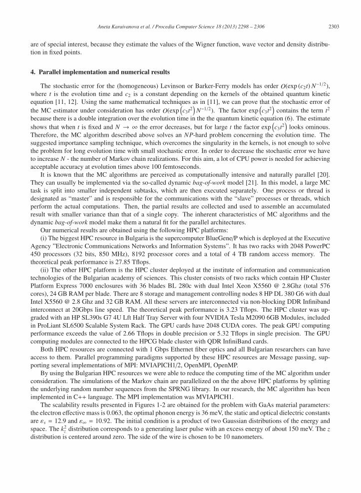
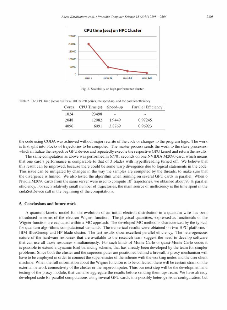
Fig. 2. Scalability on high-performance cluster.

Table 2. The CPU time (seconds) for all 800 × 260 points, the speed-up, and the parallel efficiency.

Cores CPU Time (s) Speed-up Parallel Efficiency

1024 23498 - -

2048 12082 1.9449 0.97245

4096 6091 3.8769 0.96923

the code using CUDA was achieved without major rewrite of the code or changes to the program logic. The work

is first split into blocks of trajectories to be computed. The master process sends the work to the slave processes,

which initialize the respective GPU device and repeatedly execute the respective GPU kernel and return the results.

The same computation as above was performed in 67701 seconds on one NVIDIA M2090 card, which means

that one card’s performance is comparable to that of 3 blades with hyperthreading turned off. We believe that

this result can be improved, because there could be some warp divergence due to logical statements in the code.

This issue can be mitigated by changes in the way the samples are computed by the threads, to make sure that

the divergence is limited. We also tested the algorithm when running on several GPU cards in parallel. When 6

Nvidia M2090 cards from the same server were used to compute 107 trajectories, we obtained about 93 % parallel

efficiency. For such relatively small number of trajectories, the main source of inefficiency is the time spent in the

cudaSetDevice call in the beginning of the computations.

5. Conclusions and future work

A quantum-kinetic model for the evolution of an initial electron distribution in a quantum wire has been

introduced in terms of the electron Wigner function. The physical quantities, expressed as functionals of the

Wigner function are evaluated within a MC approach. The developed MC method is characterized by the typical

for quantum algorithms computational demands. The numerical results were obtained on two HPC platforms -

IBM BlueGene/p and HP blade cluster. The test results show excellent parallel efficiency. The heterogeneous

nature of the hardware resources that are available to the research team suggest the need to develop software

that can use all those resources simultaneously. For such kinds of Monte Carlo or quasi-Monte Carlo codes it

is possible to extend a dynamic load balancing scheme, that has already been developed by the team for simpler

problems. Since both the cluster and the supercomputer are positioned behind a firewall, a proxy mechanism will

have to be employed in order to connect the super-master of the scheme with the working nodes and the user client

machine. When the full information about the Wigner function is to be collected, there will be certain strain on the

external network connectivity of the cluster or the supercomputer. Thus our next step will be the development and

testing of the proxy module, that can also aggregate the results before sending them upstream. We have already

developed code for parallel computations using several GPU cards, in a possibly heterogeneous configuration, but


we believe we should concentrate to achieve better performance from the GPU version by some code refactoring

to make the jumps more predictable.

Acknowledgment

The research work reported in the paper is partly supported by the project AComIn ”Advanced Computing for

Innovation”, grant 316087, funded by the FP7 Capacity Programme (Research Potential of Convergence Regions),

and by the Bulgarian Ministry of Education, Youth and Science under Grant DNS7FP-02/1.

References

[1] I.M. Sobol, Monte Carlo Numerical Methods, (Nauka, Moscow, 1973) (in Russian).

[2] D.P. Kroese, T. Taimre, Z.I. Botev, Handbook of Monte Carlo Methods, (Wiley Series in Probability and Statistics, John Wiley and Sons,

New York, 2011).

[3] M.A. Kalos, P.A. Whitlock, Monte Carlo Methods, (Wiley Interscience, New York, 1986).

[4] G.A. Mikhailov, New Monte Carlo Methods with Estimating Derivatives, (Utrecht, The Netherlands, 1995).

[5] I. Dimov, T. Dimov, T. Gurov, A New Iterative Monte Carlo Approach for Inverse Matrix Problem, J. of Comp. and Appl. Math., vol. 92,

pp. 15–35, 1998.

[6] Scalable Parallel Random Number Generators Library for Parallel Monte Carlo Computations, SPRNG 1.0 and SPRNG 2.0 –http://sprng.cs.fsu.edu .

[7] M. Nedjalkov, R. Kosik, H. Kosina, S. Selberherr, A Wigner Equation for Nanometer and Femtosecond Transport Regime, Proceedings

of the 2001 First IEEE Conference on Nanotechnology, IEEE, Maui, Hawaii, pp. 277-281, 2001.

[8] M. Nedjalkov, H. Kosina, S. Selberherr, C. Ringhofer, D.K. Ferry, Unified Particle Approach to Wigner-Boltzmann Transport in Small

Semiconductor Devices, Phys. Rev. B, vol. 70, pp. 115319–115335, 2004.

[9] M. Nedjalkov, H. Kosina, S. Selberherr, C. Ringhofer, D.K. Ferry, Unified particle approach to Wigner-Boltzmann transport in small

semiconductor devices, Physical Review B, 70, 115319-115335, 2004.

[10] C. Ringhofer, M. Nedjalkov, H. Kosina, and S. Selberherr, Semi-Classical Approximation of Electron-Phonon Scattering Beyond Fermi’s

Golden Rule, SIAM J. of Appl. Mathematics, vol. 64, no. 6, pp. 1933–1953, 2004, and the references therein.

[11] T.V. Gurov, P.A. Whitlock, ”An Efficient Backward Monte Carlo Estimator for Solving of a Quantum Kinetic Equation with Memory

Kernel”, Mathematics and Computers in Simulation, vol. 60, pp. 85–105, 2002.

[12] T.V. Gurov, M. Nedjalkov, P.A. Whitlock, H. Kosina and S. Selberherr, Femtosecond Relaxation of Hot Electrons by Phonon Emission

in Presence of Electric Field, Physica B, vol. 314, pp. 301–304, 2002.

[13] European Grid Infrastructure, http://www.egi.eu/.

[14] E. Atanassov, et al., SALUTE application for Quantum Transport – New Grid Implementation Scheme, Proceedings of the Spanish

conference on e-Science Grid Computing, pp. 23-32, 2007.

[15] E. Atanassov, et al., Ultra-fast Semiconductor Carrier Transport Simulation on the Grid, LSSC 2007 , Springer LNCS 4818, 461-469,

2008.

[16] M. Nedjalkov, et al., Femtosecond Evolution of Spatially Inhomogeneous Carrier Excitations: Part I: Kinetic Approach, Springer LNCS,

3743, pp. 149-156, 2006.

[17] I. Levinson, Translational invariance in uniform fields and the equation for the density matrix in the Wigner representation, Sov. Phys.

JETP, 30, pp. 362-367, 1970.

[18] M. Herbst, M. Glanemann, V. Axt, and T. Kuhn, Electron-phonon quantum kinetics for spatially inhomogeneous excitations, Physical

Review B, 67, 195305:1–18, 2003.

[19] T. Gurov, E. Atanassov, I. Dimov and V. Palankovski, Femtosecond Evolution of Spatially Inhomogeneous Carrier Excitations: Part II:

Stochastic Approach and GRID Implementation, Springer LNCS, 3743, pp. 157-163, 2006.

[20] I. Dimov, O. Tonev, Monte Carlo Algorithms: Performance Analysis for Some Computer Architectures, J. of Comp. and Appl. Mathe-matics, vol. 48, pp. 253–277, 1993.

[21] Y. Li, M. Mascagni, Grid-based Quasi-Monte Carlo Applications, Monte Carlo Methods and Appl., vol. 11, no. 1, pp. 39–56, 2005.

Documents

Monte Carlo Simulation of Ultrafast Carrier Transport: Scalability Study