MORE ON THE COST-BENEFIT ANALYSIS OF ELECTRICITY …

MORE ON THE COST-BENEFIT ANALYSIS OF ELECTRICITY PROJECTS

Arnold C. Harberger

July 2010

This paper builds on the basis of its predecessor “The ABCs of Electricity Project

Analysis”, introducing a series of additional factors that are relevant in many real-world

settings. This added relevance is bought, however, at the cost of increased complexity of

the analysis. I hope that the earlier paper will have given readers enough of an intuitive

understanding of the subject so as to permit them to incorporate these added

complications without difficulty.

Heterogeneous Thermal Capacity -- A Vintage Approach

The assumption of homogeneous thermal capacity, which was carried throughout

the previous paper, made it easy to describe what we called the “standard alternative” to

each of the types of hydro projects that were analyzed there. This assumption is

abandoned in this paper, in favor of a more realistic assumption of heterogeneous thermal

capacity. But even here there are two distinct ways of introducing heterogeneity -- one

which considers changes taking place over time in the characteristics of the thermal

plants that are being added to the system, and the other which looks at different design

characteristics of thermal plants that have different functional roles within the system.

In this section we will be concerned with the first kind of heterogeneity. Our

thermal system is here assumed to compromise plants dating from different prior years --

the oldest are assumed to be the least “thermally efficient” and therefore to have the

highest running cost per kwh. The newer is the plant, the more efficient it is assumed to

be, hence the lower will be its running cost per kwh. These assumptions lead to a

“stacking pattern” in which the newest thermal plant will be the first one to be turned on

(after run-of-the stream capacity is fully used). This will be followed by the second

newest, then the third, then the fourth newest thermal plant, in ascending order of running

cost as older and older plants are turned on. There is nothing that is difficult to

understand up to this point. It is simply an application of the idea that whatever is the

level of demand, we try to use that mix of generating equipment which satisfies that

demand at the lowest running cost.

But now we have to modify the scenario that ruled in the previous paper. There,

when we added a new plant, its natural function was to fill a “thermal peak” of demand

that would otherwise go unmet. Since the equipment being added was fully

homogeneous with the already existing thermal plants, it was right to consider this added

plant as the last one to be turned on. Now, however, we are assuming that the newest

plant is more efficient than the older ones, hence if we install it, it should be not the last

but the first thermal plant to be turned on.

This shift of function gives rise to a new possibility, namely that it may be

worthwhile to add a new thermal plant (say plant E) to an existing structure consisting

initially of plants A, B, C, and D -- even if the system demand for energy remains the

same (i.e., is not growing through time). The motive for this addition would in such a

case be exclusively the saving of running cost. The “new” system would not produce

more energy than the “old” one -- the number of kilowatt hours would not change, but the

saving in running cost might be sufficient to justify the construction of plant E.

2

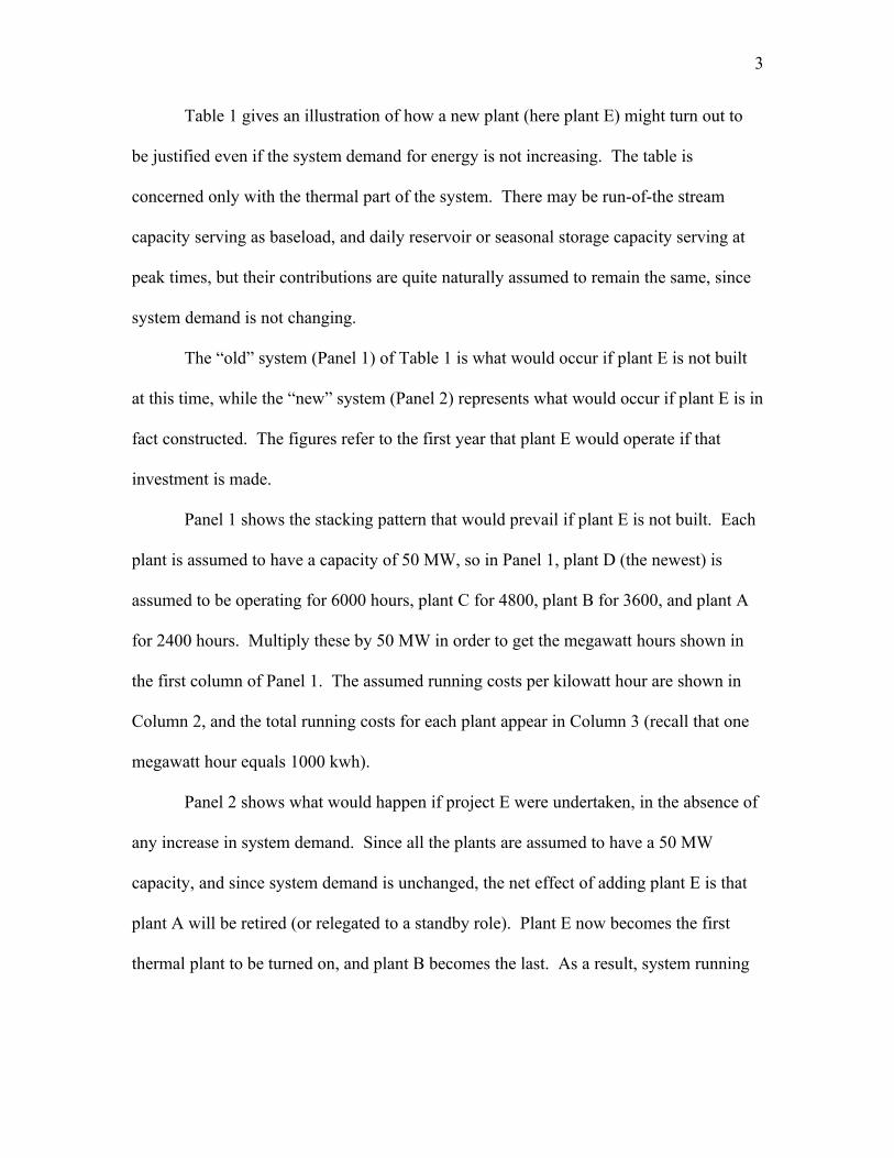
Table 1 gives an illustration of how a new plant (here plant E) might turn out to

be justified even if the system demand for energy is not increasing. The table is

concerned only with the thermal part of the system. There may be run-of-the stream

capacity serving as baseload, and daily reservoir or seasonal storage capacity serving at

peak times, but their contributions are quite naturally assumed to remain the same, since

system demand is not changing.

The “old” system (Panel 1) of Table 1 is what would occur if plant E is not built

at this time, while the “new” system (Panel 2) represents what would occur if plant E is in

fact constructed. The figures refer to the first year that plant E would operate if that

investment is made.

Panel 1 shows the stacking pattern that would prevail if plant E is not built. Each

plant is assumed to have a capacity of 50 MW, so in Panel 1, plant D (the newest) is

assumed to be operating for 6000 hours, plant C for 4800, plant B for 3600, and plant A

for 2400 hours. Multiply these by 50 MW in order to get the megawatt hours shown in

the first column of Panel 1. The assumed running costs per kilowatt hour are shown in

Column 2, and the total running costs for each plant appear in Column 3 (recall that one

megawatt hour equals 1000 kwh).

Panel 2 shows what would happen if project E were undertaken, in the absence of

any increase in system demand. Since all the plants are assumed to have a 50 MW

capacity, and since system demand is unchanged, the net effect of adding plant E is that

plant A will be retired (or relegated to a standby role). Plant E now becomes the first

thermal plant to be turned on, and plant B becomes the last. As a result, system running

3

TABLE 1

JUSTIFYING A NEW THERMAL PLANT

EVEN WHEN SYSTEM DEMAND IS CONSTANT

PANEL 1 -- “OLD” SYSTEM

Running Cost Total RunningMegawatt Hours Per kwh Cost Per Plant

Plant D 300,000 3¢ $ 9 million

Plant C 240,000 3 1/2¢ $ 8.4 million

Plant B 180,000 4¢ $ 7.2 million

Plant A 120,000 5¢ $ 6 million

Total running cost of thermal plants $30.6 million

PANEL 2 -- “NEW” SYSTEM


Plant E 300,000 2 1/2¢ $ 7.5 million

Plant D 240,000 3¢ $ 7.2 million

Plant C 180,000 3 1/2¢ $ 6.3 million



Saving of running cost = $ 4.8 million/ year

Capital cost of Plant E @ $600/KW × 50 MW = $30 million

4

costs end up lower than in Panel 1, the total saving being $4.8 million over the year. If

the capital cost of building plant E is $600/KW, for a total of $30 million for a 50 MW

plant, the project would appear to be worthwhile using the criteria applied in the previous

paper (a 10% discount rate plus a 5% rate of depreciation for the plant). The required

yearly return on capital for plant E would then be $4.5 million, while the estimated actual

return is $4.8 million.

It is worth taking time to note the composition of this $4.8 million benefit.

Simply looking at the two panels of Table 1, one sees that in Panel 2, plant E occupies the

role that plant D played in Panel 1, plant D does what C did in Panel 1, plant C occupies

the role previously played by B, and plant B does what A previously did. This is a

perfectly accurate description of the difference between the two panels, but thinking of

the new plant E as taking the place formerly occupied by plant D is not a helpful way of

describing the change. To maximize insight, we have to focus on the fact that it is plant

E that is being introduced into the system. We then have to ask, as E generates its

300,000 megawatt hours, what sources is it in effect replacing. The answer can be found

by asking what change takes place in the output of each of the other plants, as we move

from Panel 1 to Panel 2. The answer is that D, C, and B, each “lose” 60,000 megawatt

hours of output, while A loses all of its 120,000 megawatts. These “losses” add up

precisely to the 300,000 megawatt hours generated by plant E in Panel 2.

But this is only the beginning. When E supplants D for 60,000 megawatt hours,

the saving of running cost is 1/2¢ per kwh or $5 per megawatt hour. When E supplants

C, the saving is $10 per mwh, when it substitutes for B, $15 per mwh is saved. And

finally, vis-a-vis A, the saving is 2 1/2¢ per kwh, or $25 per megawatt hour. Now, as if

5

by magic, if we take ($5 × 60,000) plus ($10 × 60,000) plus ($15 × 60,000) + ($25 ×

120,000), the result is $300,000 + $600,000 + $900,000 + $3,000,000, equal precisely

(and necessarily) to the $4.8 million of saving in total cost, which we calculated directly

in Table 1. Thus the cost saving for any year t can be represented by jΣHjt(Cj-Cn),

where Cn is the running cost per kwh of the new plant, Cj is the running cost per kwh of

old plant j, and Hjt is the number of kwh for which plant j is being displaced by the

new plant, during year t.

* * * * *

The above analysis works without modification for all cases in which total

demand remains the same “with” the new plant as “without” it. However, that is a rather

special case. We get a clue as to what the general case looks like when we recall that in

the earlier paper, the output of the new plant went 100% to producing energy at the

thermal peak, and that the peaktime surcharge was actually calculated by asking what that

surcharge would have to be in order for investment in a new plant (aimed at covering the

increase in demand in the hours of thermal peak) to be justified.

What we are going to do now in Table 2 and Table 3 is to create a situation in

which investing in plant E is not justified if system demand is not increasing, but can be

justified if there is a sufficient rate of increase in system demand. Table 2 should be self-

explanatory as it simply repeats the calculation of Table 1, but with lower output for each

plant. Now, in Panel 1, plant D produces 200,000 kwh rather than 300,000. Similarly

each of the other plants has only 2/3 the output it had in Table 1. This simply would

6

reflect different demand characteristics in the system. Here D would be operating for

4000 rather than 6000 hours per year, and A would be operating for 1600 rather than

7

TABLE 2

SHOWING A CASE WHERE INVESTING IN A NEW PLANT

IS NOT JUSTIFIED WHILE SYSTEM DEMAND REMAINS CONSTANT

PANEL 1 -- “OLD” SYSTEM


Plant D 200,000 3¢ $ 6 million

Plant C 160,000 3 1/2¢ $ 5.6 million


Plant A 80,000 5¢ $ 4 million


PANEL 2 -- “NEW” SYSTEM


Plant E 200,000 2 1/2¢ $ 5 million

Plant D 160,000 3¢ $ 4.8 million

Plant C 120,000 3 1/2¢ $ 4.2 million



Saving of running cost = $ 3.2 million/ year

Capital cost of Plant E @ $600/KW × 50 MW = $30 million

8

2400. In such a system, our cost-benefit analysis would tell us to say no to plant E, if

system demand were constant through time. However, suppose demand were growing.

If we say no to plant E, we must do something to contain demand so that it stays within

the combined capacity of plants A, B, C, and D. How to do this? Via a peaktime

surcharge, of course.

For simplicity, let us assume that the thermal peak is equal to the 1600 hours that

plant A was running in Panel 1 of Table 2. Then we would derive the peaktime surcharge

by asking what peaktime surcharge it would take, in order for the “next” addition to

capacity to be justified. Using our discount rate of 10% and our depreciation rate of 5%

we would have a “required” return of $4.5 million on the investment ($30 million) in

plant E. We would have cost savings of 1/2¢, 1¢, and 1 1/2¢ with respect to plants D, C,

and B, and these would apply to 40,000 mwh each. The dollar amounts saved would be

$200,000, $400,000 and $600,000 respectively, adding up to $1.2 million. Thus plant E’s

energy at peaktime (1600 hours) would have to generate ($4.5-$1.2) million of return to

capital if the investment in E is to be worthwhile. This would be created over 1600 hours

× 50,000 KW of capacity, or 80 million kwh. The peaktime surcharge (over and above

plant B’s running cost) would then have to be $3.3 million ÷ 80 million kwh = 4.125¢ per

kwh. The peaktime price would be 8.125¢ per kwh.

The calculation would be different if the system peak were equal to, say, 1000

hours (rather than 1600). Assuming A’s turbines to be used at full capacity during this

1000 hour peak, they would produce 50,000 megawatt hours during this period. Plant E

would not be substituting for plant A during this time, but it would do so (if E is built) for

the remaining 30,000 mwh of A’s output (as shown in Panel 1). Thus Hat would be 30

9

million kwh while Hbt, Hct and Hdt would each be 40 million kwh. These

substitutions would account for a combined saving in running cost of $1.95 million (=

$200,000 + $400,000 + $600,000 for plants D, C, and B, as before, plus $750,000 for

plant A, covering the 30,000 mwh that we have calculated for Hat). In order to generate

the $4.5 million of benefits that are required to justify investing in plant E, the peaktime

surcharge (over A’s running cost of 5¢) would have to generate benefits of $2.55 million

(= $4.5 million minus $1.95 million). Per kwh, this “surcharge” would be 5.1¢ per kwh.

The peaktime price of energy in this case would be $10.1¢/kwh.1

Readers should be aware that the peaktime “prices” that we calculate here do not

in any way have to be put into practice (i.e., be actually collected from the power

company’s customers). They really are measures of the actual economic cost of bringing

peaktime energy in line by way of constructing plant E. Our $4.5 million figure reflects

the economic cost of the capital invested in plant E. If plant E only worked at peaktime

one would have to assign this full $4.5 million of capital cost to the peak period. In our

case, the bulk of this cost is being covered by savings of running cost during the offpeak

1

In this calculation we assume that the timing of plant E’s introduction into the system would be such that even in E’s presence both A and E would be fully utilized during the 1000 hours of system peak. This gives rise to the question, how is the system managed during the interval in which system peak demand exceeds 200 MW (the sum of the capacities of A, B, C, and D) but falls short of 250 MW (where all five plants would be operating at capacity). The economist’s answer to this question is that the peaktime price of energy would move up gradually from 3¢ (= A’s running cost) to 8.4¢ (the level that would justify introducing plant E). The object of such a gradually increasing peaktime price would be to contain peak demand within the 200 MW limit, until the point where the introduction of plant E is optimal. This answer, however, involves too much fine-tuning for the practical world. The practical solution is simply to set the peaktime price at 7.9¢ soon as system peak demand threatens to exceed 200 MW at a price of 3¢, and then introduce plant E at the point where it can fully substitute for plant A.

10

period. The peaktime price we calculated represents the remaining part of this cost, and

thus reflects the true cost of supplying peaktime energy via the investment in plant E.

Thus we would use the peaktime prices that we have calculated to measure the

benefits of a daily reservoir project’s adding to the supply of energy at a system peak of

1000, or the benefits of a seasonal hydro project’s increasing the supply of energy during

a system peak of 1600 hours. The underlying purpose of our calculating peaktime prices

based on thermal costs is therefore to give us a cost-based way of assigning a value to

peaktime energy coming from alternative sources of energy.

Thermal Capacity That Differs by Type of Plant

In this section we will consider differences in the capital and running costs of

thermal plants, based on their physical (engineering) characteristics. For simplicity, we

will confine out examples to three types of facility -- big thermal, combined cycle and gas

turbine. There used to be many more relevant variations by type, as there would be

significant variations in capital and running costs for coal-fired plants of different sizes.

This sort of variation has been greatly reduced as a consequence of the introduction of

combined cycle generating plants. These plants use petroleum or natural gas as fuel, and

use jet engines or similar equipment to generate energy in the first cycle. The second

cycle then uses the heat produced in the first cycle in order to create steam, which then

produces additional energy in the second cycle. Once combined cycle technology came

onto the scene, it turned out to be the cheapest way of generating electricity under a very

substantial range of demand conditions. Thus our choice of just three types of generating

equipment pretty well reflects the realities of contemporary thermal power industries.

The characteristics of our three types of equipment are:

11

Capital Cost (K) Annualized Capital Running Cost Cost (= .15×K)

Big Thermal $2000/KW $300 $200 per KW/yr

Combined Cycle $1200/KW $180 5¢ per kwh

Gas Turbine $ 600/KW $ 90 9¢ per kwh

Readers will note that the running costs of big thermal are expressed on an annual

basis per KW of capacity, rather than on a per-kilowatt-hour basis. The reason for this is

that big coal-fired units cannot be turned on and off to meet variations in system demand.

As is the case with nuclear capacity, turning them on and off is a costly operation, leading

to their characteristic use as baseload capacity which only gets turned off for maintenance

and repairs.

Table 3 examines the total annual costs of using these three types of capacity in

order to meet different durations of energy demand. It is easily seen there that big

thermal is the most efficient way to meet an annual energy demand (per KW of installed

capacity) lasting 7500 hours, while combined cycle is best for a demand covering 5000

hours in the year, and also for one covering 3000 hours. For demands lasting 2000 and

1000 hours, however, gas turbines provide the most efficient answer.

If different types of capacity are best for different numbers of hours, there have to

exist critical numbers of hours marking the “borderline” between two types. These

borderlines are found by equating the total costs for two adjacent kinds of capacity. Thus

at 6400 hours the total annualized cost of combined cycle capacity is equal to $180 +

$.05(6400) = $500, exactly the same as the full-year cost ($300 + $200) of a KW of big

thermal capacity. Demands with durations longer than 6400 hours can thus be

accommodated most cheaply by big thermal capacity, while new demands lasting

12

TABLE 3

ELECTRICITY SYSTEM INVESTMENT DECISIONS WITH

THREE DIFFERENT TYPES OF GENERATING CAPACITY

Annualized Running Costs Total Costs/KWCapital Costs/KW Per Year Per Year

Use for 7500 hours/yr. Big Thermal $300 $200 $500 Combined Cycle $180 5¢×7500 = $375 $555 Gas Turbine $90 9¢×7500 = $675 $765

Use for 5000 hours/yr. Big Thermal $300 $200 $500 Combined Cycle $180 5¢×5000 = $250 $430 Gas Turbine $ 90 9¢×5000 = $450 $540




Borderline between big thermal and combined cycle$300 + $200 = $180 + .05 N1$320 = $.05 N1

6400 = N1

Borderline between combined cycle and gas turbine$180 + .05 N2 = $90 + .09 N2

$90 = (.09-.05) N2

13

2250 = N2

14

somewhat less than 6400 hours can be more efficiently served by combined cycle

capacity. These answers apply a) when the new demand stands alone (i.e., when we are

building capacity just to satisfy this demand) and b) when the new demand is added to

an already optimized system.

In an exactly analogous fashion we can find that the borderline between combined

cycle and gas turbine capacity is 2250 hours. For this number of hours, total annual costs

of combined cycle capacity amount to $180 + (2250 × 5¢), or $292.50, exactly the same

as the annual total for at capacity, equal to $90 + (2250 × 9¢) = $90 + 202.50 = $292.50.

So again, either for a stand-alone demand or for a new demand within an already

optimized system, we would install GT capacity for demands lasting less than 2250

hours, and combined cycle capacity for demands going up from this point.

Table 4 explores cases in which capacity is being added to an already optimized

system. The first step is to identify system marginal costs -- these are equal to 3¢/kwh,

the marginal running costs of big thermal, when it is the most expensive capacity at work

(i.e., during hours of quite low system demand). Similarly, system marginal costs equal

5¢/kwh when combined cycle is the most expensive capacity at work (i.e., during periods

of intermediate system demand). Then we have system marginal costs equal to 9¢/kwh

when gas turbine capacity is marginal. These are times when the system’s big thermal

and combined cycle plants are all operating at full capacity, and therefore have to be

supplemented by gas turbines in order to accommodate the system’s full demand. The

system marginal cost of 9¢ occurs when this is the case and when the system’s gas

turbine capacity is not fully utilized -- i.e., when the system is not yet at peak demand.

15

Now consider the fact that if gas turbine plants were to generate revenues of 9¢

per kwh for all their hours of operation, this would just cover their running costs, but

would make no contribution to their capital costs. Thus, just as in the previous paper the

peaktime surcharge was in a first example set at 6¢ and a thermal peak surcharge in a

later example was set at 3¢ in order to cover the annualized capital cost of new

homogeneous thermal capacity, we now set a peaktime surcharge of 9¢, in order to cover

the annualized $90/KW capital costs of gas turbine capacity, over a system peak of 1000

hours per year.2

In Table 4 we deal with three cases, each dealing with how the system should

respond to a new set of energy demands -- Case #1 considers a new demand with a

duration of 7000 hours per KW per year; Case #2 considers a new demand lasting 4000

hours; and in Case #3 the new demand has a duration of 1500 hours. These cases

illustrate how, in an optimized system of the kind we are working with, a) each new

demand can be met by its appropriate type of capacity, and b) when this is done and that

new capacity is remunerated at system marginal cost for each hour that it runs, the total

remuneration precisely covers the sum of annualized capital costs plus annual running

costs for the appropriate type of capacity.

2

When we deal with peaktime in this paper, we act as if the relevant capacity (here gas turbines) is absolutely fully utilized over the assumed duration (here 1000 hours) for peak demand. In reality, an electricity administration would define peaktime hours in a very sensible way (say 5-11 p.m. for a lighting peak in winter, 8-11 p.m. in summer) fully recognizing that the GT part of the system would not be operating at absolutely full capacity during these times. The rest of the system (big thermal and combined cycle) would, however, be at full capacity. Setting the peaktime surcharge at precisely 9¢ turns out to “right” from the standpoint of big thermal and combined cycle capacity; as is shown in Table 4. It is also “right” from the standpoint of GT capacity if it is indeed fully used for the 1000 hour peak. This is what we assume here. An upward modification of the peaktime surcharge would lead to excess rewards for big thermal and combined cycle.

16

Thus, in Case #1, big thermal is the “right” capacity to meet a new demand for

7000 hours a year. If it earns system marginal costs, it will get 18¢/kwh during1000

peaktime hours, 9¢/kwh during 1250 hours, 5¢/kwh during 3750 hours, and finally

3¢./kwh during the 1000 hours when big thermal is the system’s marginal capacity. As is

shown for Case #1 remuneration at these marginal costs will precisely cover by thermal’s

annualized capital costs of $300/KW plus its annual running cost (at 7000 hours) of 7000

× 3¢ = $210/KW.

Similarly, in Case #2 we have combined cycle capacity being built to

accommodate a new demand lasting 4000 hours per year. Here remuneration at system

marginal cost covers 1000 hours at 18¢ plus 1250 hours at 9¢ plus 1750 hours at 5¢ per

kwh. The total of these “earnings” is $380 per KW per year, which precisely equals the

sum of an annualized capital cost of $180/KW plus a running cost of 5¢/kwh for 4000

hours in the year.

Finally, Case #3 explores a new demand lasting 1500 hours, and met by adding

new gas turbine capacity. Here that capacity “earns” 18¢/kwh for 1000 hours and

9¢/kwh for 500 hours for a total of $225/KW per year. Once again, this amount precisely

covers the GT annualized capital cost of $90 per KW plus the GT running cost of 9¢/kwh

for 1500 hours per year.

It almost looks like a “miracle” that a single peaktime surcharge turns out to be

the only supplement to system marginal running cost that is needed, in order to fully

cover both capital and running cost of each type of capacity in a fully optimized system.

17

TABLE 4

INVESTMENT POLICY IN A SYSTEM WITH OPTIMIZED

CAPACITIES AND SYSTEM PEAK OF 1000 HOURS

System Marginal Costs

Big Thermal Capacity -- Operates for 6400 hours or more. System Marginal Costs when Big Thermal Operation is the marginal capacity = zero

Combined Cycle Capacity -- Operates for more than 2250 hoursand less then 6400 hours when this is the system’s marginal capacity. System marginal costs = 5¢/kwh

Gas Turbine Capacity -- Operates for less than 2250 hours peryear. When this capacity is only partially used (not at system peak),System marginal costs = 9¢/kwh

Peaktime Surcharge -- Sufficient to cover capital costs of gasturbine capacity during 1000 hours of system peak. Annualized capitalcosts of $90.00 ÷ 1000 peaktime hours = peaktime surcharge of 9¢/kwh.System marginal cost during 1000 peaktime hours = 9¢ running cost +9¢ peaktime surcharge = 18¢/kwh

Case #1: New demand arises (new factory working 3 shifts per day), operating for 7000 hours per year.

Answer: build big thermal capacity to meet this demand “earns” 18¢/kwh during 1000 peaktime hours = $180 “earns” 9¢/kwh during 1250 hours when

gas turbine is marginal capacity = $112.50“earns” 5¢/kwh during (6400-2250) = 4150 hours

when combined cycle is marg. corp. = $207.50“earns” zero during 1000 hours when big thermal is marginal capacity = 0 Total “earnings” = $500

Cost of this new capacity = $300 annualized corp. cost + $200running cost = $500

Big Thermal’s costs are exactly covered by system marginal costs including peaktime surcharge.

18

19

Table 4 (continued)

Case #2: New demand arises (new factory working 2 shifts per day), operating for 4000 hours per year.

Answer: build combined cycle capacity to meet this demand “earns” 18¢/kwh during 1000 peaktime hours = $180 “earns” 9¢/kwh during 1250 hours when

gas turbine is marginal capacity = $112.50“earns” 5¢/kwh during (4000-2250) = 1750 hours = $87.50 Total “earnings” = $380

Cost of this new capacity = $180 annualized Capital cost + 5¢ × 4000 hours = $200running cost = $380

Case #3 -- New demand arises (population growth leads to new residential demand plus commercial and street lighting), operating for 1500 hours per year.

Answer: build gas turbine capacity to meet this demand“earns” 18¢/kwh during 1000 peakload hours = $180“earns” 9¢/kwh during 500 hours when

gas turbine is marginal capacity = $ 45 Total “earnings” = $225

Cost of this new capacity = $90 annualized capital cost + 9¢/kwhduring 1500 hours = $225

20

Perhaps with an excess of zeal I have called this proposition “the fundamental theorem

of modern electricity pricing” At any rate, it was a noteworthy discovery in the annals of

electricity economics.

As we shall see, a system which follows the rules of marginal cost pricing will

tend over time to approach an optimized level. But many of the world’s systems fall far

short of this point at the present time and probably will still be non-optimized for quite

some time into the future. In most of these cases the non-optimality of the system stems

from two sources -- a) the presence of older steam and gas turbine plants that will

naturally be retired as they live out their economic lives, and b) the fact that combined

cycle technology has not had enough time to reach the levels needed for a fully optimized

system. Table 5 explores two cases, both dealing with a system that does not net have its

optimal amount of combined cycle capacity. These cases deal, respectively, with

increases of demand of long (7000 hours) and short (1000 hours) duration. These new

demands would “normally” (i.e., in a fully optimized system) be met by adding,

respectively, big thermal capacity (for the 7000 hour increment of demand), and gas

turbine capacity (for the 1000 hour increment). However, because of the non-optimality

of the system, it turns out that the best response, even to these very long-duration and

very short-duration increments of demand, is to add combined cycle capacity. This

strategy is not only the cheapest way of accommodating the new demands; it also moves

the system closer to optimality.

In Case #4, the new demand has a duration of 7000 hours. At first glance it seems

natural that this demand should be filled by big thermal, which is the most efficient type

of capacity for demands of this length. That is true in an optimized system. But in a non-

21

TABLE 5

INVESTMENT POLICY IN A NON-OPTIMIZED SYSTEM

WITH “TOO LITTLE” COMBINED CYCLE CAPACITY

• System has “too much” big thermal capacity, which ends up satisfying demands of 4500 hours or more.

• System has “too much” gas turbine capacity, which ends up satisfying all demands of 3000 hours or less.

• System has “too little” combined cycle capacity, which ends up satisfying demands between 3000 and 4500 hours per year. Recall that, combined cycle capacity has an economic advantage (based on capital and running costs.) for demands all the way from 2250 to 6400 hours per year. So quite naturally, if a new demand arises within the 2250-6400 range, it should be filled by adding combined cycle capacity. However, owing to the non-optimality of the system, it turns out that the answer to any increase in demand is to add combined cycle capacity, as this brings the system closer to an optimum. The following examples show why this is so.

Case #4 -- New demand arises for 7000 hours per year.Answer: Meet this demand by taking away big thermal from its “margin” at 4500

hours per year and shifting it to satisfy the new demand of 7000 hours. No capital cost or marginal running cost is involved since this capacity operates full time in either case.

Now add combined cycle capacity to fill the void of 4500 hourscreated by shift. This entails $180 of annualized capital cost plus4500 × 5¢ = $225 of additional running cost = $405

Total Cost of meeting new demand = $405

Total cost of meeting this new demand by directly buildingbig thermal capacity for this purpose = $300 annualized capitalcost plus $200 of annual running cost = $500

Hence -- It is cheaper to add combined cycle than to install new big thermal capacity to meet this new demand.

22

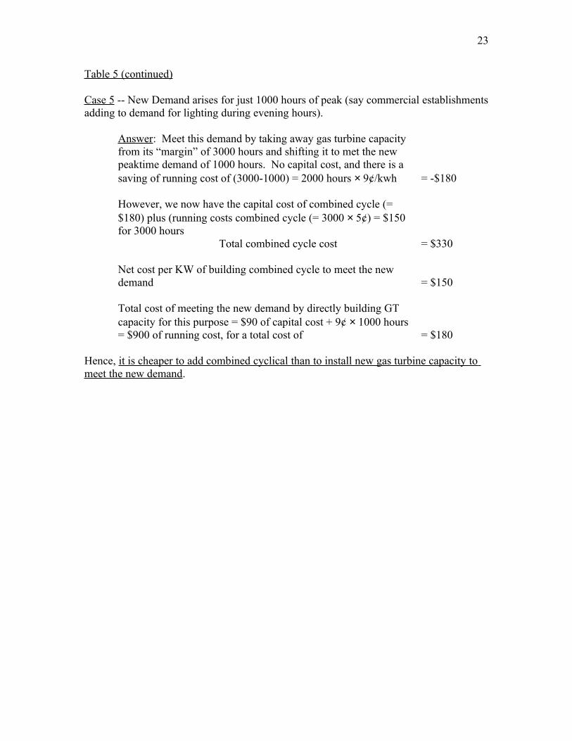
Table 5 (continued)

Case 5 -- New Demand arises for just 1000 hours of peak (say commercial establishments adding to demand for lighting during evening hours).

Answer: Meet this demand by taking away gas turbine capacityfrom its “margin” of 3000 hours and shifting it to met the new peaktime demand of 1000 hours. No capital cost, and there is asaving of running cost of (3000-1000) = 2000 hours × 9¢/kwh = -$180

However, we now have the capital cost of combined cycle (= $180) plus (running costs combined cycle (= 3000 × 5¢) = $150for 3000 hours

Total combined cycle cost = $330

Net cost per KW of building combined cycle to meet the newdemand = $150

Total cost of meeting the new demand by directly building GTcapacity for this purpose = $90 of capital cost + 9¢ × 1000 hours= $900 of running cost, for a total cost of = $180

Hence, it is cheaper to add combined cyclical than to install new gas turbine capacity to meet the new demand.

23

optimized system we may already have some big thermal capacity doing what it

shouldn’t (optimally) do. This is true in our Case #4, where we have some big thermal

capacity that is meeting demands of only 4500 hours a year. The right answer is to shift

this big thermal capacity out of this slot (where it doesn’t belong), to move it to the new

7000 hour slot (where it does belong) and to replace it in the 4500 hour slot by combined

cycle capacity, which is optimal for that duration. As the table shows, this set of moves

meets the new demand at a total (capital plus running) cost that is lower than the cost of

meeting the new demand with new big thermal capacity.

Similarly, we have Case #5, of a new demand with a duration of just 1000 hours.

This is taken to be at peaktime, because if it were away from the peak this new demand

could be met by simply making more intensive use of the system’s existing capacity.

Here the casual observer might think that the best way to respond to the new demand

would be to add new gas turbine capacity. Again, this would be the right answer if the

system was starting from an optimized position. But given the non-optimality of having

some GT capacity working as long as 3000 hours, the best answer is to shift this GT

capacity to the new 1000-hour slot. This saves 9¢ × 2000 hours of GT running cost per

KW of shifted capacity. To replace this shifted GT capacity in the 3000 hour slot, we

introduced new combined cycle capacity, having an annualized capital cost of $180 and

an annual running cost of $150 (= 3000 × 5¢). The total cost of this CC operation is

$330 per year, but deducting the saving of running cost on the shifted GT capacity, we

find a net cost of $330 - $180 = $150. This is obviously lower than the $180 cost of

satisfying the new 1000 hour demand by adding new gas turbine capacity.

24

Cases #4 and #5 show why it is true that in a non-optimized system that has too

little combined cycle capacity, adding to that particular type of capacity will be the cost-

minimizing way of responding to new demands of essentially any duration.

SOME NOTES ON SOLAR AND WIND POWER

The right way to think about solar and wind power is to consider them as the

modern counterparts of run-of-the-stream generation. All of these have the characteristic

that the ultimate source of energy experiences natural variations that are beyond our

direct control. In the case of run-of-the-stream projects, we have the possibility of adding

daily reservoirs, at which point we do control the flow of energy into the system. The

counterpart of daily reservoirs would be to use wind or solar energy to pump water from

a lower to a higher level, with the intention of generating electricity through hydro

turbines during peaktime hours. This is known as pump storage, and involves two dams,

one above and the other below the incline down which the water flows to the turbines.

Pump storage projects have existed at least since the 1930s, but they have not become

very widespread because of the heavy capital costs that they involve. Aside from pump

storage, another means of controlling the flow of electricity from wind and solar sources

would be through batteries -- generate electricity as the wind and sun permit, but use

batteries to store that energy, so that it can be used at times of high value per kilowatt

hour. To our knowledge, such use of batteries is still far from being cost-effective.

Thus our discussion of wind and solar energy will concentrate on the standard

case, directly analogous to run-of-the-stream projects, where the electricity generated by

the project is delivered to the system at the time and in the volume determined by the

whims of nature.

25

Solar and wind projects differ from run-of-the-stream operations in that one does

not always encounter diminishing returns to adding turbines or solar panels at a given

site. Ten solar panels will catch ten times as much sunlight as one panel, and ten turbines

will catch ten times as much wind as one of them (with some exceptions in cases of

canyons, etc. which channel the wind in special ways). The generating capacity of solar

and wind projects will therefore be determined mainly by the costs of installing more

turbines or panels, and by the needs of the electricity system.

The standard way of dealing with capacity of these kinds is to assign to their

output the relevant system marginal costs. Reverting to our example of Table 4, suppose

a solar or wind project had a maximum output of 10MW. To value its expected output

for any future year we would first assign system marginal costs for each hour of

operation. Thus, following Table 4, we would have 2360 (= 8760 - 6400) hours at zero

marginal cost (when big thermal was expected to be the marginal capacity), 4150 hours at

5¢ (when combined cycle was expected to be at the margin), and 2250 hours at 9¢, the

marginal running cost of gas turbine capacity. These add up to $410 per KW per year.

However, the solar or wind project would be expected to operate only at a fraction of its

capacity, owing to fluctuations in the availability of wind and sunlight. We here assume

the relevant fraction to be 30%, which reduces the benefit to $123 per KW of capacity.

The above calculations assign no part of the peaktime surcharge to the wind or

solar project. This is because in both cases there are likely to be many peaktime hours

during which the project will have zero output. In order to meet peaktime demand at

such times, some sort of other standby capacity would have to be available. This might

consist of older capacity, mainly retired from the system but held for standby purposes

26

for just this kind of contingency. But within the framework of Table 4, it would be gas

turbine capacity. There may be places where the wind or sun is so reliable that it can be

counted on, at a specified intensity, in peaktime hours. If we assume that intensity to be

20% of the maximum intensity, then we would add to the above figure of $123, an

amount equal to 20% of the 9¢ peaktime surcharge, times the 1000 hours of peaktime

use. This would add $18; for a total benefit of $141 per KW.

Some discussions of wind and solar power speak of a “necessity” of

supplementing these projects with backup peaking capacity (which in our case would be

gas turbines). These discussions focus on the unreliability of these sources to provide

peaktime power. The backup capacity enters the picture in order to fill precisely this

role. We feel that such “packaging” is unnecessary. In coming to this conclusion we rely

on a fundamental principle of project evaluation -- namely, the principle of “separable

components”. This principle says that if we have two projects X and Y, we can define

their combined benefit (in present value) as Bx+y, their separate, stand-alone benefits as

Bx and By and the benefits of each, conditional on the presence of the other, as Bxy

and Byx. It is easy to see that:

Bx+y = Bx + By x = By + Bx y

Similarly, for costs:

Bx+y = Cx + Cy x = Cy + Cx y

Now if the “joint project” (X+Y) is the best option, this means that

(Bx+y-Cx+y) > (Bx-Cx)

(Bx+y-Cx+y) - (Bx-Cx) > 0

27

and therefore By x > Cy x .

That is, if the joint project is acceptable, project Y must pass the test as the marginal

project -- it must be worthwhile to add project Y to an initial package consisting only of

project X.

Similarly, it can be shown that if the joint project is best, project X must pass the

test as the marginal project -- it must be worthwhile to add project X to an initial

package consisting only of project Y.

There is no escaping the rigorous mathematical logic of this argument. If a

package consisting of a wind project and a backup GT project is the best option. Then

each of these two components must pass the cost-benefit test as the marginal project,

measuring its contribution as what it would add (to benefits and costs, respectively) in the

presence of the other. We therefore must evaluate a wind or solar project as being

additional to any GT or other standby peaking project with which some would argue it

ought to be “packaged”.

28

POSTSCRIPT

In this and the preceding paper, the main objective is to convey an understanding

of the underlying economic principles that characterize the provision of electric energy.

The starting point is that the value of the kilowatt hour -- the standard “product” that

electricity customers buy and consume -- will normally exhibit wide variations by hour of

the day and season of the year. This occurs in spite of the fact that there is probably no

item more physically homogenous from unit to unit than kilowatt hours of 120 volts and

60 cycles. The reason for the variation in value stems from different effective marginal

costs of providing energy at different times. When an electricity system is not working at

capacity, the effective marginal cost is the highest running cost among the different plants

that are operating at the time. As plants are turned on, in ascending order of running cost,

the effective marginal cost will be low at times of low demand, and high at times of

heavy demand on the system’s resources. System marginal cost is highest at peak

periods, because here the true cost must also cover a provision for capital cost recovery of

the type of capacity that has to be expanded when peaktime demand increases.

The key to evaluating investments in new generating capacity is to value their

expected output at “system marginal cost”, at each moment they are expected to operate.

Put another way, the benefits that are to be expected from a new plant are the costs that

will be saved due to its presence in the system. This is something that seems

straightforward and easy to understand, but in fact it is anything but simple. The

subtleties arise because the output of a new plant stretches many years into the future, so

the bulk of its cost-saving will take place then. The principle guiding the estimation of

these future cost savings is that year by year and into the future, the system will continue

29

to follow good cost-benefit principles as it retires old plants and invests in new ones.

Any given plant will almost certainly have a trajectory of benefits that starts high, and

then declines over time. For thermal plants, one can expect that future additions will be

more efficient than the current ones, so that today’s new plant, which may start as the

most efficient one of its class, may end its life as the least efficient of the class, having

been bumped from a heavy load factor (high hours of use) at the beginning of its life to

lower and lower hours of use as time goes on. Finally, it will be relegated to standby

capacity, and ultimately to the scrap heap. Hydro storage dams have a similar trajectory

of benefits, in this case stemming from their inevitable accumulation of mud and silt. As

this occurs, their effective storage capacity inevitably declines. Perhaps run-of-the-

stream projects and daily reservoirs (which can be desilted quite easily) are the only ones

whose benefit streams may escape an inevitable downward drift through time.

The downward trend of benefits of a given project is incorporated in our analysis

via an allowance for depreciation. Investment in an asset that does not depreciate can be

justified if that asset just yields the required rate of return (opportunity cost of capital). It

is the expectation of declining (or ultimately terminating) benefits that leads to first-year

benefits covering more than the required rate of return. The use in our exposition of a

required rate of return-plus-depreciation in the first year of a project’s operating life is

intended to capture all of the subtleties referred to in this note.

The fact that the future benefits of electricity projects are measured by their

expected savings of costs gives rise to another possibility -- that the electricity system in

question may have already in place a modern and highly sophisticated system of cost

control and future investment programming. That is to say, those enterprises or public

30

authorities may already have done a lot of the work needed in order to see how a given

new plant will fit into the system, and which particular costs it will likely be saving, hour

by hour and year by year, at least for a few years into the future. All we can say here is

that, as cost-benefit analysts, we should be grateful when such pieces of luck relieve us of

a great deal of work!!

31

Documents

MORE ON THE COST-BENEFIT ANALYSIS OF ELECTRICITY …