Embed Size (px)
Citation preview
ATMO 595EDecember 2, 2004
MRF Boundary Layer Parameterization
Melissa Goering

Outline• Background for MRF PBL
scheme• WRF Input data
– Constants (WRF and MRF PBL subroutine)
• MRF Output data• Equations
– Troen and Mahrt 1986– Hong and Pan 1996 – Businger et al., 1971– Brost and Wyngaard 1978
• Sensitivity Analysis

Basic MRF PBL ParameterizationVertical diffusion scheme MRF (prior 1996)
– There is no explicit boundary layer parameterization– Diffusivity coefficients are parameterized as functions of
the local Richardson number– Thus the local-K approach (by Louis 1979) is used for
BOTH boundary layer and free atmosphere– Widely used because computationally cheap and
produces reasonable results under typical atmospheric conditions
– However, the scheme cannot handle conditions when atmosphere is well mixed because of the countergradientfluxes. Thus, the method is not well behaved for unstable conditions.

Basic MRF PBL ParameterizationConcept adapted by Troen and Mahrt, 1986*:
– Develop model where transport of mass and momentum in PBL is accomplished by large scale eddies and modeled by bulk properties of PBL instead of local prosperities
– Turbulent diffusivity coefficients are calculated from prescribed profile shape as function of boundary layer heights and scale parameters derived from similarity requirements
– Utilizes the results of the large-eddy simulation research and is computationally efficient
* Businger et al. 1971; Brost and Wyngaard 1978; Wyngaardand Brost 1984; Holtslag and Boville 1993;

Free Atmosphere: Local-K approach
Nonlocalmixing

WRF Input DataU3D 3D u-velocity interpolated to theta points (m/s)V3D 3D v-velocity interpolated to theta points (m/s)TH3D 3D potential temperatures (K)T3D temperature (K)QV3D 3D water vapor mixing ratio (kg/kg)QC3D 3D cloud mixing ratio (kg/kg)QI3D 3D ice mixing ratio (kg/kg)P3D 3D pressure (Pa)PI3D 3D exern function (dimensionless)rr3D 3D dry air density (kg/m^3)RUBLTEN U tendency equation to PBL (m/s^2)RVBLTEN V tendency equation to PBL (m/s^2)RTHBLTEN Theta tendency equation to PBL (K/s)RQVBLTEN Qv tendency equation to PBL (kg/kg/s)RQCBLTEN Qc tendency equation to PBL (kg/kg/s)RQIBLTEN Qi tendency equation to PBL (kg/kg/s)P_QI species index for cloud icedz8w dz between full levelsz height above sea level (m)

PSFC pressure at surface (Pa)ZNT roughness length (m) [land=0.10, water=0.001]UST u* in similarity theory (m/s)ZOL z/L height over Monin-Obukhov length HOL PBL Height over Monin-Obukhov lengthREGIME flag indicating PBL regime (stable, unstable,etc)PSIM similarity stability function for momentumPSIH similarity stability function for heatXLAND land mask (1= land, 2 = water)HFX upward heat flux at the surface (W/m^2)QFX upward moisture flux at the surface (kg/m^2/s)TSK surface temperature (K)GZ10Z0 log(z/zo) where zo is roughness lengthWSPD wind speed at lowest model level (m/s)BR bulk Richardson number in surface layerDT time step secondsDTMIN time step minutes
WRF Input Data (continued)

WRF Input ConstantsROVCP R/CPR gas constant for dry air (J/kg/K)G acceleration due to gravity (m/s^2)ROVG R/G XLV latent heat of vaporization (J/kg)RV gas constant for vaporization (J/kg)rvovrd R_v divided by R_d (dimensionless)SVP1 constant saturation vapor pressure (KPa)SVP2 constant saturation vapor pressure (dimensionless)SVP3 constant saturation vapor pressure (K)SVPT0 constant saturation vapor pressure (K)EP1 constant for virtual temperature (Rv/Rd -1), 0.608EP2 constant for specific humidity calculation, 0.628KARMAN Von Karman constantEOMEG angular velocity of earth’s roation (rad/s)STBOLT Stefan-Boltzman constant (W/m^2/K^4)

MRF PBL subroutine ConstantsBRCR = 0.5 Critical Bulk Richardson numberRLAM = 150 Asymptotic length scale 250m,
Hong and Pan1996 to 30mRImin = -100.0 Local gradient Ri to prevent unrealistic unstableZFmin = 1x10⁻⁸ Minimum value allowed in equation Kzm, (1 – z/h)PRmin = 0.5 Prandtl number bounded 0.5 < Pr < 4.0PRmax = 4.0XKZmin = 0.01 Diffusivity coef. bounded between 0.01 < Kz <1000 m2s-1
XKZmax = 1000.0CFAC = 7.8 thermal excess b in equation based on observationPFAC = 2.0 exponential p in equation based on observationPRT = 1.0Alpha5 = 5.0 constant in equation based on observationAlpha16 = 16.0 constant in equation based on observationCKZ = 0.001XKA = 2.4x10⁻⁵SFCFRAC = 0.1

MRF PBL subroutine Output DataU2DTEN u tendency calculatedV2DTEN v tendency calculatedT2DTEN temperature tendency calculatedQV2DTEN water vapor tendency calculated QC2DTEN cloud tendency calculatedQI2DTEN ice tendency calculatedKPBL1D boundary layer height (m)
PSIM similarity stability function for momentumPSIH similarity stability function for heat
HFX upward heat flux at the surface (W/m^2)QFX upward moisture flux at the surface (kg/m^2/s)TSK surface temperature (K)ZNT roughness length (m)UST u* in similarity theory (m/s)ZOL z/L height over Monin-Obukhov length HOL PBL Height over Monin-Obukhov lengthREGIME flag indicating PBL regime (stable, unstable, etc)

MRF Equations• Nonlocal Diffusivity: Mixed layer
– Stable Regime – Unstable Regime
• Calculation PBL• Local-K approach: Free Atmosphere
– Stable Regime – Unstable Regime
• Where did constants come from?– Kansas 1968– Minnesota 1973

Nonlocal DiffusivityθT-virtual temperature excess
near the surface, maximum limit of 3K
h – is the boundary layer height and determined iteratively; Ribcr =0.5
Ws – the mixed layer velocity scale, where UST calculated
γc – countergradient calculated for θ and q, where b=7.8; term is small stable conditions
Calculate tendency
stable

Nonlocal Diffusivity
Kzm Kzh = Kzm / Pr
Turbulent velocity scale Prandtl number
Friction velocityMonin-Obukov length
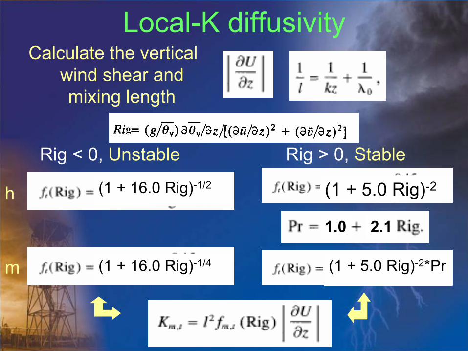
Local-K diffusivity
g
1.0 2.1
Rig < 0, Unstable Rig > 0, Stable
Calculate the vertical wind shear and mixing length
(1 + 5.0 Rig)-2
(1 + 5.0 Rig)-2*Pr(1 + 16.0 Rig)-1/4
(1 + 16.0 Rig)-1/2h
m

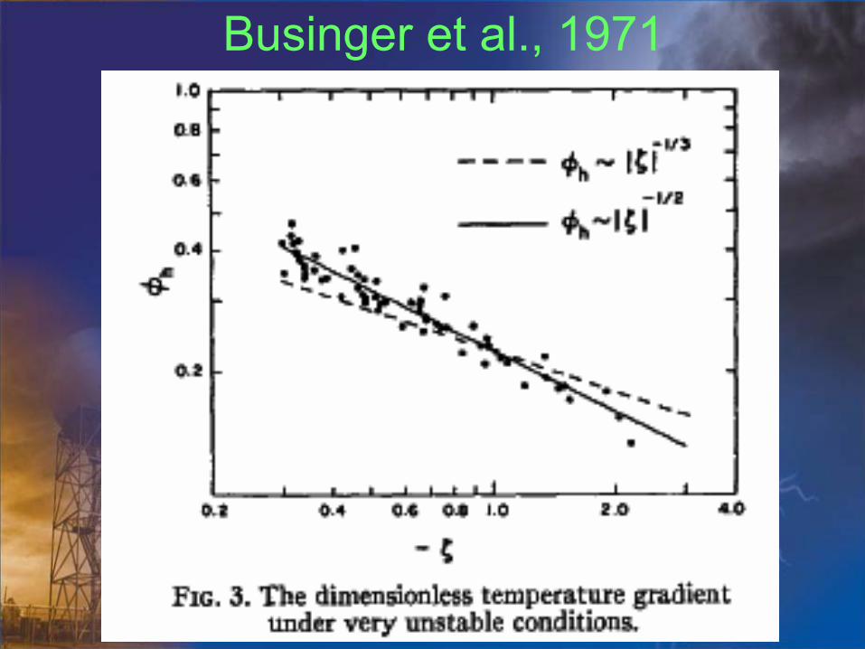
Kansas 1968 (Businger et al., 1971)– site located in wheat farming country of
southwestern Kansas – 32m tower located in center of one mile
square field of wheat stubble ~18cm tall– Analyses suggest surface roughness length
of ~2.4cm, zero plane displacement of ~10cm– 34 runs analyzed with basic average period
15min
Where did they get those constants?

Businger et al., 1971
< Unstable >
< Stable >
StableUnstable Unstable Stable
Businger et al., 1971

Sensitivity AnalysisEvaluate role of countergradient term by removing
thermal excess (b=0.0):
– Removing thermal excess (b=0.0), the nonlocal turbulent mixing due to the γc plays a role in stabilizing the structure and creates a deeper boundary layer depth (more clearly in mixing ratio)
– However, the γc is not fully responsible for difference between local and nonlcoal and the cubic shape is also important in the nonlocal scheme
– Found that the impact of nonlocal mixing due to mixing ratio γc effect was negligible (no figure)

Hong and Pan, 1996

Sensitivity AnalysisEvaluate role of
countergradient term by increasing thermal excess b=[ 7.8,11.7 ]:
– Including the γcterm plays a significant role in simulating the well-mixed boundary layer structure BUT the magnitude only minor influence
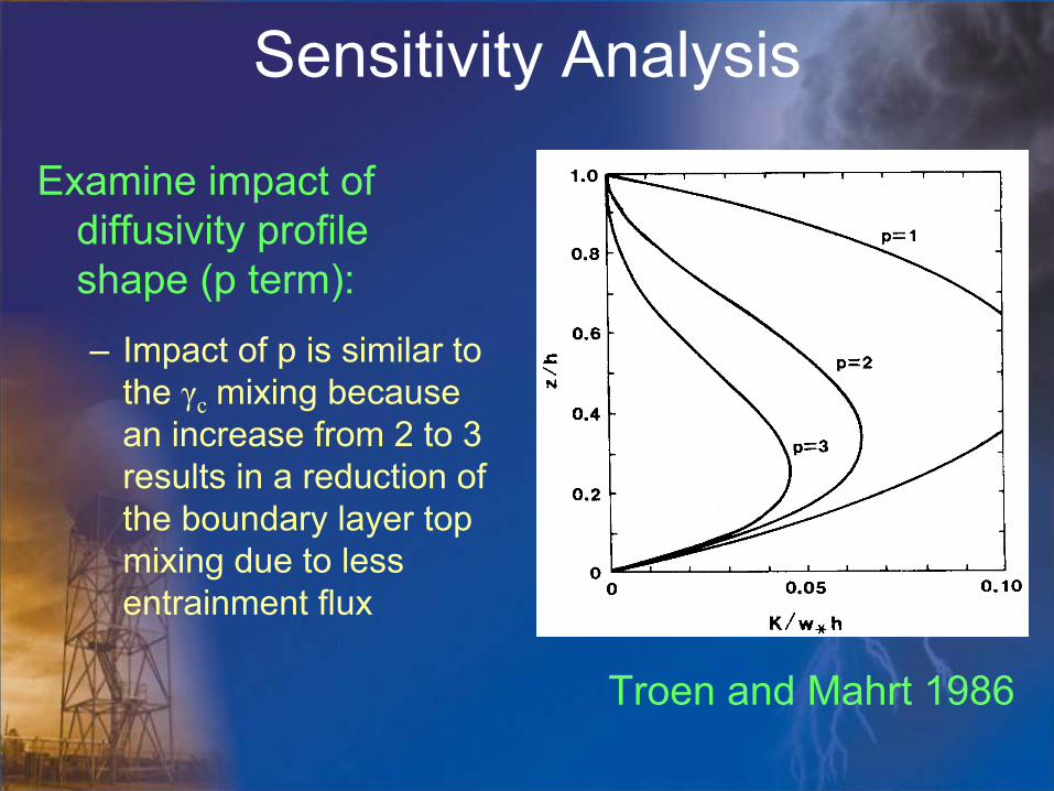
Sensitivity Analysis
Examine impact of diffusivity profile shape (p term):
– Impact of p is similar to the γc mixing because an increase from 2 to 3 results in a reduction of the boundary layer top mixing due to less entrainment flux
Troen and Mahrt 1986

Sensitivity AnalysisSensitivity of boundary layer height on critical
Richardson number:– Impact of Ribcr in precipitation forecast was found to be
significant on heavy rain case for 15-17 May 1995
– Less effective mixing with lower PBL height (due to lower Ribcr) most likely leads to similar precipitation as local scheme
– However, nonlocal experiment with Ribcr = .75 shows more organized precipitation and more effective mixing and gives favorable boundary layer structure
– As surface heating decreases, Ribcr becomes more important in determining PBL depth which results in different BL top entrainment
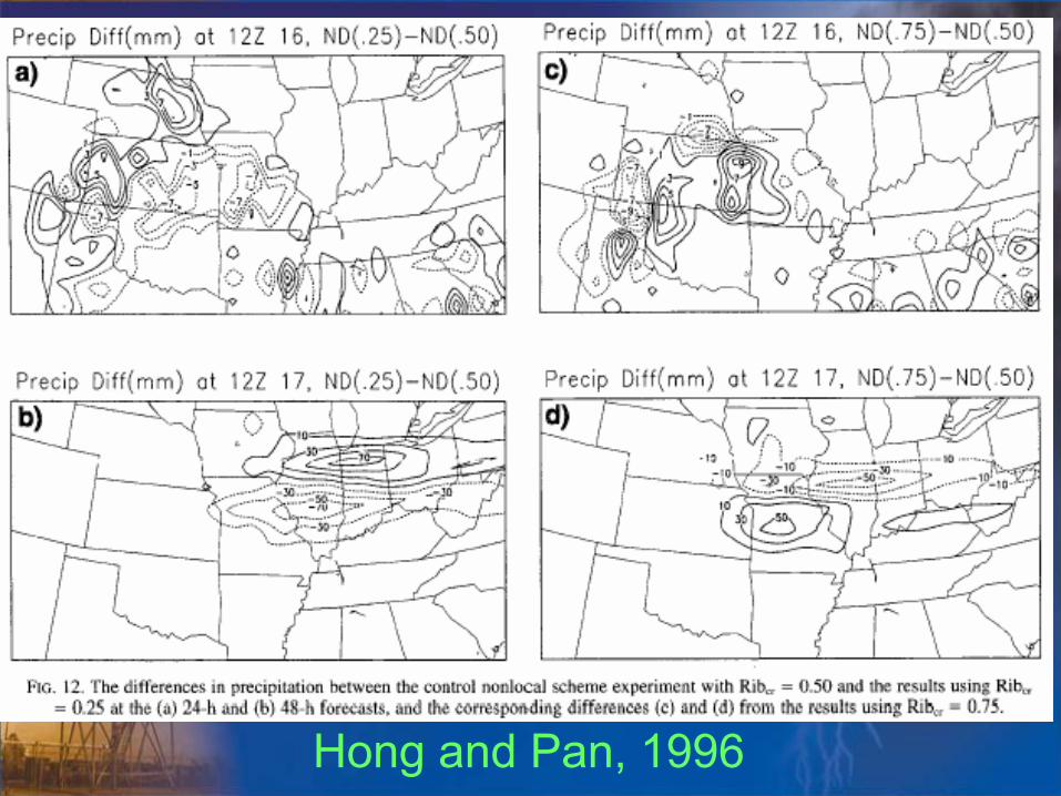
Hong and Pan, 1996

Hong and Pan, 1996

Summary MRF PBL parameterization
• Local diffusion scheme uses eddy diffusivity determined independently at each point in the vertical based on local vertical gradients wind and virtual potential temperature
• Nonlocal scheme determines eddy-diffusivity profile based on diagnosed BL height and turbulent velocity scale and it incorporates the nonlocal transport effects of heat and moisture (γc)
• MRF PBL equations derived from “Golden days” observations taken either from Kansas 1968 (Businger et al., 1971) or Minnesota 1973 (Kaimal et al., 1975).

Summary MRF PBL parameterization
• Impact on BL structure shows Ribcr and thermal excess (b) are negligible compared to the countergradient term and p factor for profiles of potential temperature and mixing ratio BUT not the same for precipitation field
• In the heavy precipitation case, Hong and Pan (1996) found that the rainfall is significantly affected by modifying the Ribcr, p profile, and countergradient term.
• However, should be able to tune the scheme by changing Ribcr only to get reasonable precipitation forecasts

ReferencesTroen and Mahrt, 1986: A Simple Model of the Atmospheric Boundary
Layer; Sensitivity to Surface Evaporation. Bound. Lay. Met., Vol. 37, pg. 129-148.
Hong and Pan, 1996: Nonlocal Boundary Layer Vertical Diffusion in a Medium Range-Forecast Model. Mon. Wea. Rev., Vol. 124, pg. 2322-2339.
Brost and Wyngaard, 1978: A Model Study of the Stably Stratified Planetary Boundary Layer. J. Atmo. Sci., Vol. 35, pg. 1427-1440.
Businger et.al, 1971: Flux-Profile Relationships in the Atmospheric Surface Layer. J. Atmo. Sci., Vol. 28, pg. 181-189.
Holtslag and Boville, 1993: Local Versus Nonlocal Boundary Layer Diffusion in a Global Climate Model. J. Atmo. Sci., Vol. 6, pg. 1825-1842.
Wyngaard and Brost, 1984: Top-Down and Bottom-Up Diffusion of a Scalar in the Convective Boundary Layer. J. Atmo. Sci., Vol. 41, pg. 102-112.
Wyngaard, 1975: Modeling the Planetary Boundary Layer - Extension to the Stable Case. Bound. Lay. Met., Vol. 9, pg. 441-460.
WRF model Browser Code: http://box.mmm.ucar.edu/wrf/WG2/wrfbrowser/

Questions?
ATMO 595EDecember 2, 2004
Melissa Goering