MS-R-7704

AN APPROACH TO THE LIMITED APERTURE PROBLEM OF

PHYSICAL OPTICS FARFIELD INVERSE SCATTERING

by

Robert D. Magert and Norman Bleistein

Mathematics Department, College of Arts & Sciencesand

Mathematics Division, Denver Research Institute

University of Denver

. A - -

This research was supported by the Office of Naval Research.

t Present address: Mathematics Department

Colorado School of MinesGolden, Colorado 80401

0. CT 1-

Abstract

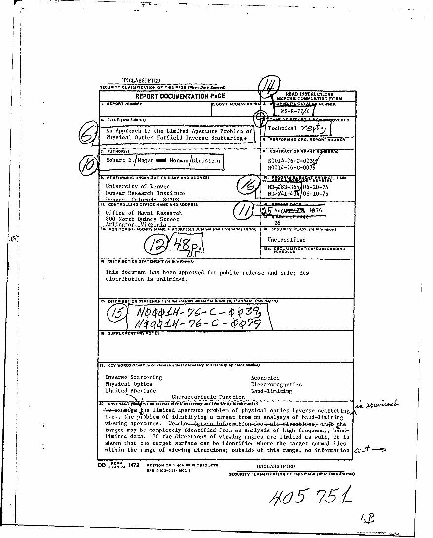
We examine the limited aperture problem of physical optics

farfield inverse scattering, i.e., the problem of identifying a

target from an analysis of band-limited viewing apertures. We

show (given inf(- mation from all directions) that the target may

be completely identified from an analysis of high frequency, band-

limited data. If the directions of viewing angles are limited as

well, it is shown that the target surface can be identified where

the target normal lies within the range of viewing directions;

outside of this range, no information is available. It is shown

that this phenomenon is totally a feature of the Fourier transform

of characteristic (non-zero) functions and independent of the

inverse scattering formalism. Numerical examples are given for the

case of a perfectly reflecting circular cylinder

All-p

1. Introduction.

Physical optics inverse scattering constitutes a technique

whereby the shape and locatic- of an acoustical or electromagnetic

scattering target may be determined from an analysis of back-

scattered, far-field data. The fundamental identity of the method

(first discovered by Bojarski, [1]) relates a quantity p+(K)

(that is proportional to the back-scattering cross-section of

radar analysis), to the Fourier transform of the characteristic

function of the scattering target; i.e., a function which is unity

inside the target, and zero outside.

The key assumptions leading to the Bojarski identity are

(1) that the target may be modelled as an acoustically hard or

soft reflector (or as a perfect conductor in the electromagnetic

case); (2) that the physical optics approximation is valid for

the back-scattered fields; and (3) that the source and observation

ranges are large compared to a typical target dimension. The

fundamental identity, which is derived briefly in Appendix A

for the reduced wave equation, states that

OV~+ + P_(-D_r+() = -2 (1.1)

K2

where r(X) is the target characteristic function, and r(_) is

its Fourier transform. In this expression, the transform vector

_c is given by

K_ 2kX k =c'(1.2)c

Below, we shall use the alliteration POFFIS for "Physical OpticsFarfield Inverse Scattering".

|-57

2

where k is the wave propagation number, w is the (time-harmonic)

frequency, and c is the propagation speed; the vector X is a

unit vector pointing in the direction of the source-observation

position. The symbol (*) denotes complex conjugation.

Therefore, if r(c) could be measured for a sufficiently large

class of vectors K, one could in principal determine r(X) by

direct Fourier inversion. As (l.2)clearly implies, this would

necessitate that measurements be performed at all frequencies and

at all aspect angles with respect to the target about which informa-

tion is desired.

An immediate difficulty which arises with the method, there-

fore, is the lack of complete information in transform space; the

physical optics approximation is valid only in the high-frequency

regime, i.e., as the wavenumber k approaches infinity. Further-

more, data that would be available from an actual experiment would

most likely be confined to some band-limited spectrum. A further

limitation cf the POFFIS method occurs because data can

seldom be measured at all aspect-angles with respect to

the unknown target.

These difficulties lead to the limited-aperture

problem o the POFFIS method -- the problem of identifying

the target structure from the limited knowledge of r(!) in K-space.

The objective of this paper -s to present solutions to the limited-

aperture problem for a physically reasonable class oZ frequency

and aspect-angles limited apertures.

774 r- 7--__

3

We show (given information from all directions) that the target

may be completely identified from an analysis of high-frequency,

band-limited data. If Lne aperture is limited in aspect angles as

well, it will be shown that the target surface can be unambiguously

determined at those points where the outward normal to the target

surface lies within the range of directions defined by the aperture

in K-space. Outside of this range, no information is possible by

this method.

The limited-aperture problem has been previously examined

(from an analytical standpoint) by Lewis E2] and Perry [3]. Lewis

considered a number of aspect-angles limited apertures, with the

(physically unreasonable) assumption that information was available

for all frequencies. Perry concluded that the absence of low-

frequency information leads to an ill-posed problem which is numer-

ically unstable. The primary difficulty is that the low-frequency

data constitutes a principal contribution to the gross resolution of

the function r().

Additional tests of Bojarski's results were carried out numeri-

cally in papers by Tabbara [4, 5] and Rosenbaum-Raz [6]. Their re-

sults confirm the difficulties with resolution due to bandlimiting.

One purpose of this paper is to show how this shortcoming of the

method can be overcome.

The key feature of the method we describe here is that we re-

place the problem of determining F(X2) by the problem of determining

the directional derivative of r(x) in some direction . The

directional derivative • Vr(X) is a highly singular function

whose essential features can be resolved from an analysis of high-

A

frequency data. The process of differentiating in the direction

q

4

in X-space corresponds to multiplication by K • in K-space; in

this way, one simultaneously suppresses low-frequency data while en-

hancing high-frequency data. Indeed, this approach was first sug-

gested in Bojarski's initial work [1], and the present work supports

and extends his ideas.

In section (2) are displayed a numbcr of computer-generated

examples for a variety of limited-data apertures. These examples

were generated from the exact back-scattered, far-field data which

was numerically computed according to a scheme by Greenspan and

Werner [7].

We remark that the advantage gained by calculating the Fourier

transform of a directional derivative is wholly a feature of Fourier

analysis. It has nothing to do with Bojarski's physical optics

identity, nor has it anything to do with the discretization and

specific calculation technique (FFT in this work) used in the in-

version of the transform. It is shown in Section 3 by asymptotic

methods why the band-limited transform behaves as it does.

More precisely, in two dimensions, we express the band-limited

inverse Fourier transform of the directional derivative as a three-

fold integral in arc length over the boundary of the target, and

K and 0 , the magnitude and angle of the transform vector K

Under the assumption of high frequency band-limiting, the first and

third of these integrals can be calculated asymptotically by the

method of two-dimensional stationary phase [8]. The integration

in magnitude K is carried out exactly. The result of this cal-

culation explains the qualitative features of the numerical results

Multiplication by higher powers of K, correspona to higher derivatives,further subdues the effect of low frequence data and further enhances

the effect of high frequency data.

5

shown in Section (2). Furthermore, stationary phase analysis brings

out the features of the aspect-angles problem, as well; namely, given

a certain range of aspect angles in transform space, the inverse

transform is asymptotically of lower order outside of the analogous

aperture in physical space.

The extension of this analysis to the case of three dimensions

is discussed in Appendix B.

494

W

6

2. Numerical Results

Figures (2.1-8) display the results of the method. They were

generated in the following way. The reduced wave equation was

solved for a point source in the exterior of a totally reflecting

circular cylinder by a method due to Greenspan and Werner [7]. The

phase and range normalized backscattered amplitude (defined below

(A.11) in the Appendix) is calculated to five place accuracy. This

is then substituted into Bojarski's basic identity (1.1) to yield

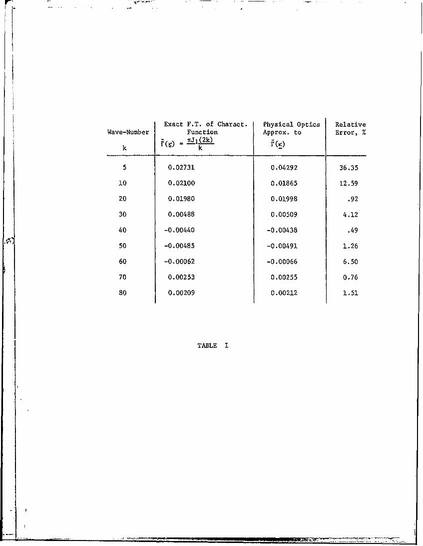
I'(K) . Table I compares the exact Fourier transform for the target

cross-section with that predicted by the inverse diffraction tech-

nique. Agreement is poor for wave numbers below ka = 10, emphaiz-

ing the need for high frequency, band-limited analysis. We remark

that the source-observation range was 25 radii, indeed in the far

field, so that this could not have accounted for the discrepancy at

moderate values of ka.

The backscattered data was used in the formula

V '(X) = (27r) 2 Ki ( K K) ei ' dK , (2.1)

for the directional derivative of the characteristic function.

Here the domain of integration is all of K-space. In particular,

we chose

= (1,0) , (2.2)

corresponding to transverse differentiation of r(X) , an proceed to

calculate (2.1) over finite domains representing band-limited and

7

aspected-angles limited apertures.

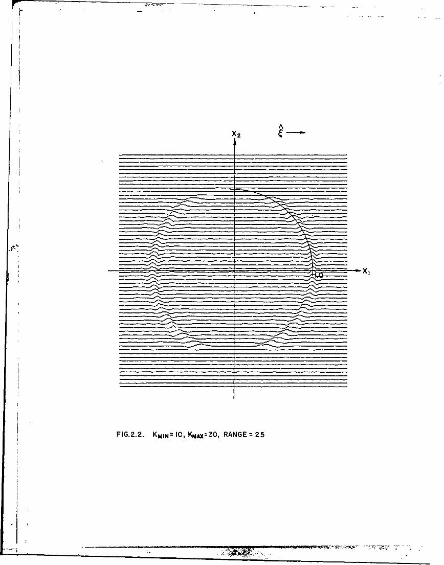
The inverse transform is calculated via a fast-Fourier trans-

form (FFT) routine. Band-limited data around k = 10, 20 and

was used, with a mesh size of 128 x 128 (of which most entries were

zero) and mesh-widths AK = AK2 = 1.1 . The resulting function

was then computer-displayed to yield the graphical results shown

in Figures (2.1-7).

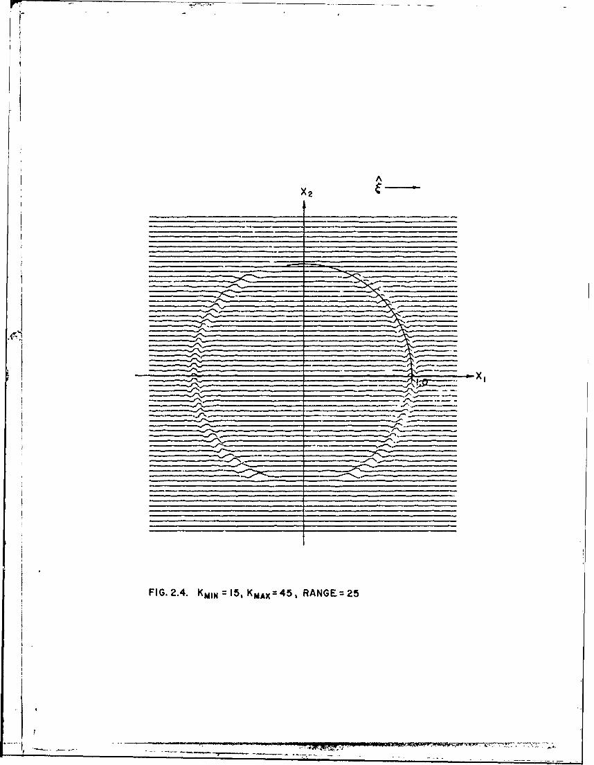
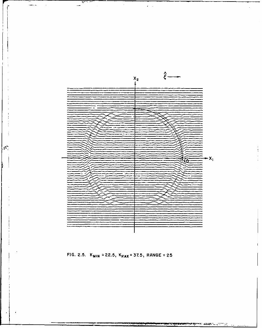
The resolution in those diagrams is seen to be approximately

one-half the minimum wavelength associated with the domain of inte-

gration in K . The clarity of the results is also seen to be

directly a function of the frequency band-width, as expected.

Furthermore, we believe that better resolution may be attained by

curve fitting the actual output to the results predicted by the

asymptotic analysis in the next section. The "smearing" effect

near the lower and upper portions of the target is due to the fact

that we calculate the transverse derivative of r(X), and this

derivative approaches zero at these limits. This minor shortcoming

maybe overcome in one of the following ways: (i) calculating a direc-

tional derivative which does not vanish in these Amits (different

A

multiplying by K2 rather than F, •K before inverting the Fourier

transform).

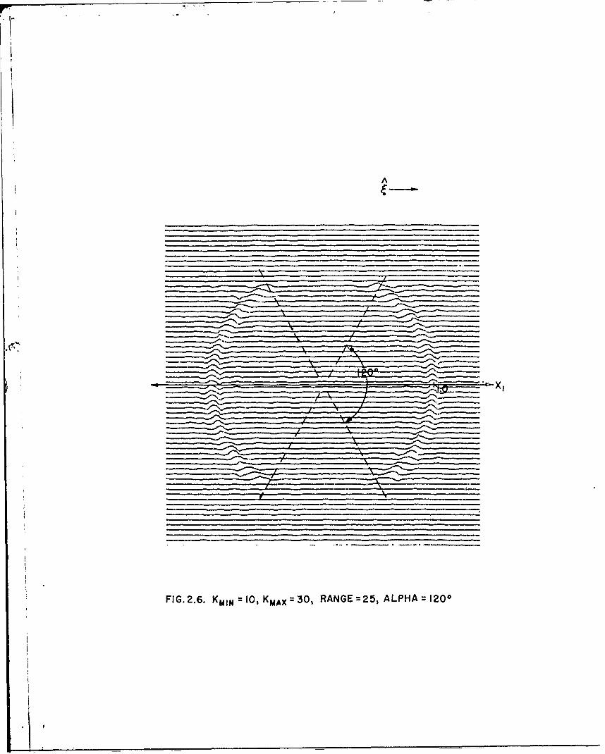
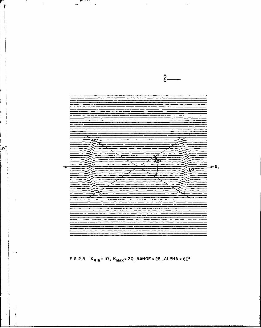
Figures (3.5-7) show the results from a viewing aperture which

is limited in direction, as well. The theory developed in the next

section will predict good resolution of the target surface where

the outward normal to the target lies within the family of directions

8

specified by the viewing aperture; outside of this range no infor-

mation is availabl(.

One further remark is due concerning the computer plotting

results. The theory developed in the next section is based upon

leading order asymptotic effects. There are also secondary effects,

corresponding to boundary integral contributions, etc., but these

do not appear due to normalization in the plotting process.

I- '3

9

3. Limited Aperture Analysis

We proceed in this section with an analysis of the integral

(2.1). Let us denote the region of K-space where the measuredA

function P(K) is known by D , and the characteristic function of

D by A(K)

A(K) = { I SD0 K D

We consider the function

A A

Kr(K) .K (3.1)

This is the Fourier transform of the directional derivative of

r(x) in the 9 direction. We note that the product of rl(K)

and the aperture function A(K)

A A i

H(K, ) = A(K) ?(I) , (3.2)

is known everywhere in K-space. We consider first the two-dimen-

sional version of (3.2) (Applicable when the target is known to be

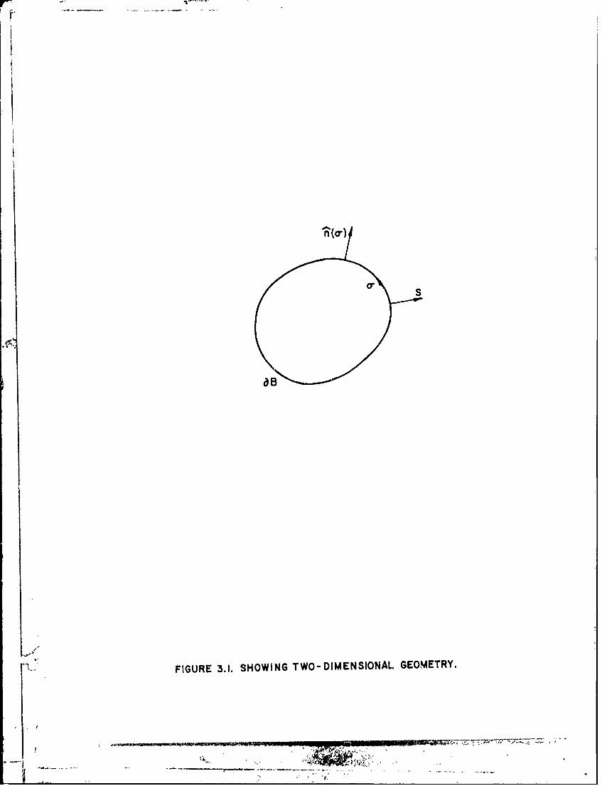
a cylinder whose cross-sectional profile is sought). We introduce

as new coordinates arc length a along the boundary curve B

and distance normal to the boundary, denoted by s (see Figure

(3.1). The directional derivative, AX) , may be represented as

r I(X) v • r(x) n • 6n(s).

Here = fi(a) is the outward unit normal to DB . A Fourier in-

version of (3.1) and use of the convolution theorem for Fourier

.. _ __ .

10

transforms leads to

1I(, 1 - (27)-2 ( "a) A(X- X'(a))da (3.3)3B

The objective of this analysis is to evaluate k3.3) asymptoti-

cally in the high frequency limit, i.e., for K = target anywhere

in D . We use the explicit representation of A(X)

A(X) = JJ eiK'! dK

D

to rewrite (3.3) as

H(K,) (27f da n(a) • J eiX--'( ))dK (3.4)

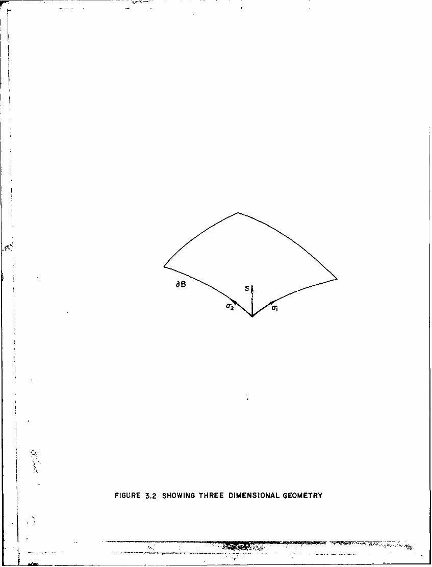
DB DA. The three-dimensional analogue of (3.4) is

H(X,) (21r)3 f da n(cy) f J' di'(X-X'())dK, (3.5)

BB D

where a (c1,V02) represents surface coordinates over aB (Figure

(3.2)). Analysis of (3.5) is carried out in Appendix B and we

proceed with the analysis of (3.4) here.

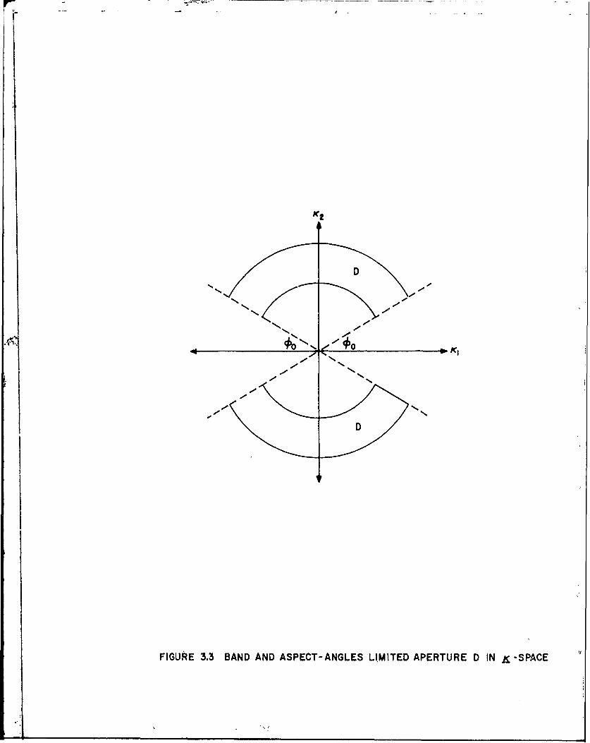
Consider an aperture which is limited in both frequency and

directions, as illustrated in Figure (3.3); note that the K-space

aperture D must be symmetric about the origin by virtue of the

analysis leading to the physical optics identity (Appendix A,

equation (A.13)).(When the aperture directions are restricted to

one-sided viewing, it is possible to extend the data symmetrically

through the origin in K-space; the reconstructed image will then

be symmetric in physical space (Lewis [ 2]), and one has no informa-

tion concerning the opposite side of the target.)

Define K = KK , where K and K are the magnitude and

directions of K , and rewrite (3.4) as

I,

(3.6)K

21) f fK 0 B SID

0

the angular integration in this expression is described by the

parameter 0, which is taken to be the angle of the vector K.

With the assumption that K0 > 1, the expression in (3.6)

may be examined via a stationary phase analysis in the variables

(o,G). With the phase function (D(a,O) defined by

((a,o) = K(o) • -X '(a))

the stationary phase conditions become

dX(o)-K(0) T(o) = 0 , T- , (3.7)

a do dK(e)(0) • x- X '(a)) 0 , t(o) = . (3.8)

do

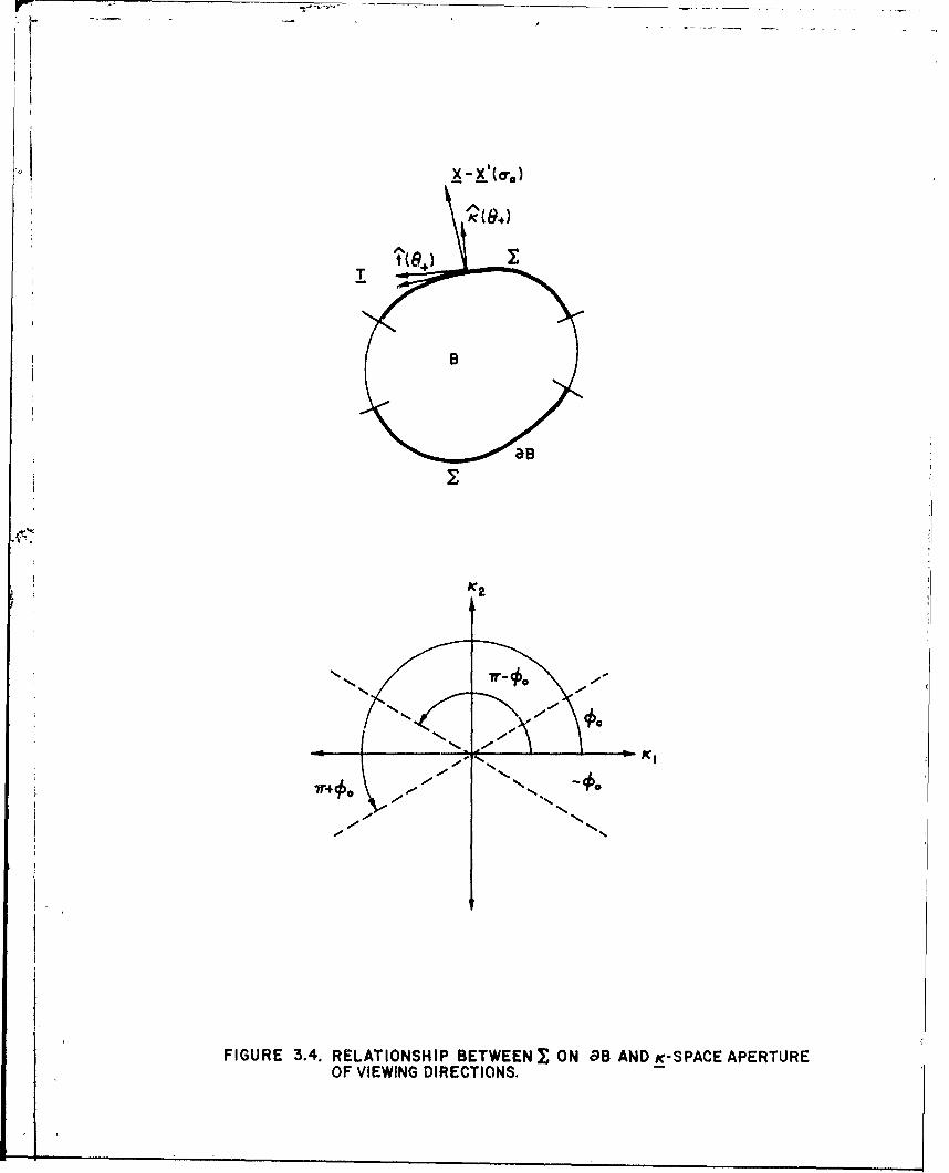
Let E represent the portion of the surface aB where the family

of normals n(o) lie within the range of directions specified by

the aperture D. Then the conditions (3.7) and (3.8) will be satisfied

in E when the vector X - X' (a) is orthogonal to the tangentA

vector T to DB, and when K(O) is collinear with X - '(o),

as illustrated in figure (3.4).

Since the K-space aperture is symmetric about the origin, there

exist two solutions, 0 = 0+, for which

A t

K(0 ) = K(_) . (3.9)

+

There may also exist a multiple of solutions in the arc-length

variable a; however, it will be evident from further analysis

12

that the stationary point a = a for which (X - V (a)) is am

minimum will dominate.

Define the two-dimensional Hessian matrix H bye

H = det[$(a,6)]e

we note that

dX'(a ( 2H= -IX -X'()IxC0 -Ie -- d

In this expression, X = X(a ) is the curvature of the targetm

surface aB at =a , and

+1 XeB

(-1 X B

With these identifications, H(X, ) is asymptotically equal to

K0

that is,

^n(am) " ( Sin(1clx- X'(am)Il) - Sin(KoIX- X'( 1 m)I) 1

H (X, g^a) - __________ ___

tha is

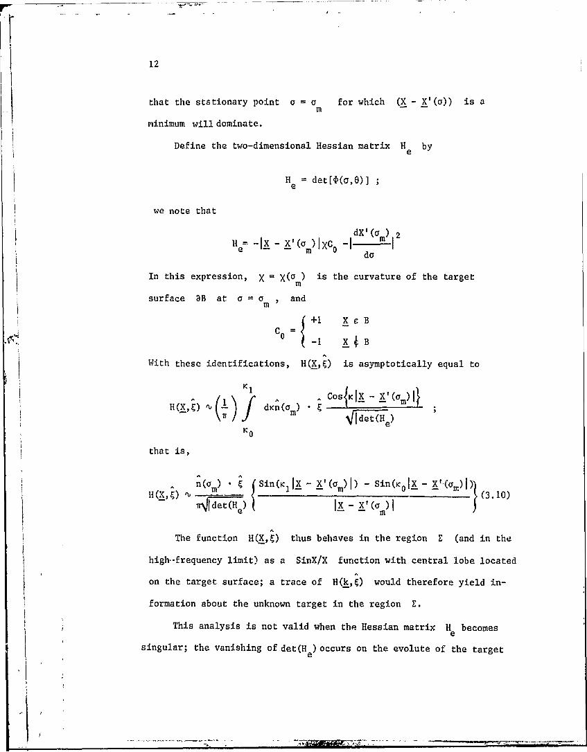
The function H(X,!) thus behaves in the region E (and in the

high-frequency limit) as a SinX/X function with central lobe located

on the target surface; a trace of H(k,g) would therefore yield in-

formation about the unknown target in the region E.

This analysis is not valid when the Hessian matrix H becomese

singular; the vanishing of det(H e) occurs on the evolute of the target

-. 11 • - - = ii --------------- ml -w• -"r-..

13

surface 3B. These are stationary points of higher order. However,

one can verify that the amplitude at those points is zero and hence

the contribution from such a sLationary point is lower order than

the contributions derived above.

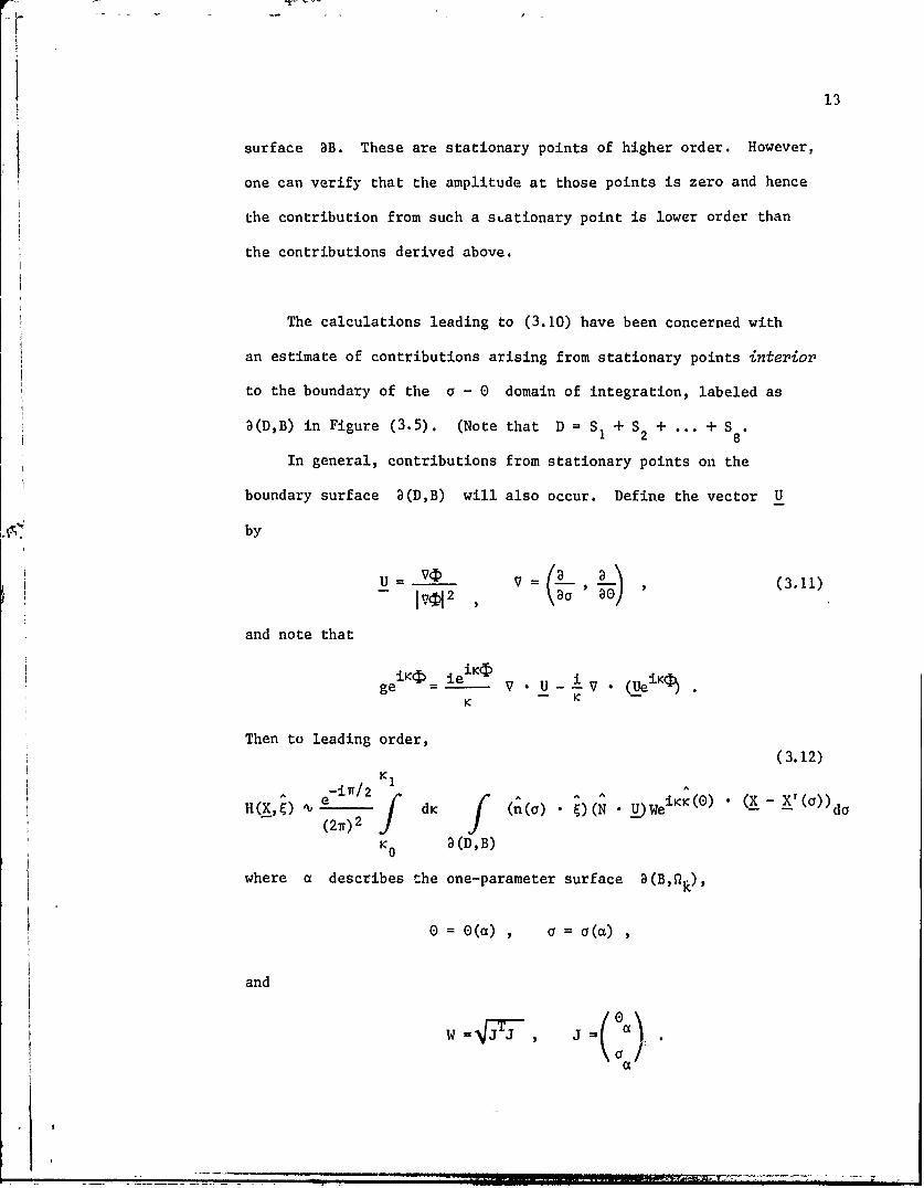
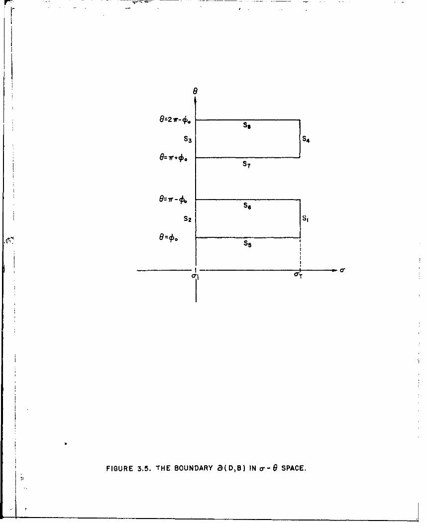
The calculations leading to (3.10) have been concerned with

an estimate of contributions arising from stationary points interior

to the boundary of the a - 0 domain of integration, labeled as

D(D,B) in Figure (3.5). (Note that D = S + S2 + ... + S8

In general, contributions from stationary points on the

boundary surface 3(D,B) will also occur. Define the vector U

by

U = , , (3.11)

and note that

iKc- ieiK i (UeiK .ge -V U U -V •Ui(

K - K

Then to leading order,(3.12)

KA -iT/2 WiK (0) (X ())d

H(X, ) , e dK (n(a) •-(N • U(2v) 2

Ko D(D,B)

where a describes the one-parameter surface a(B,)

0 = 0(a), a = a(a)

and (°o)W= , = ,a

14

* ts

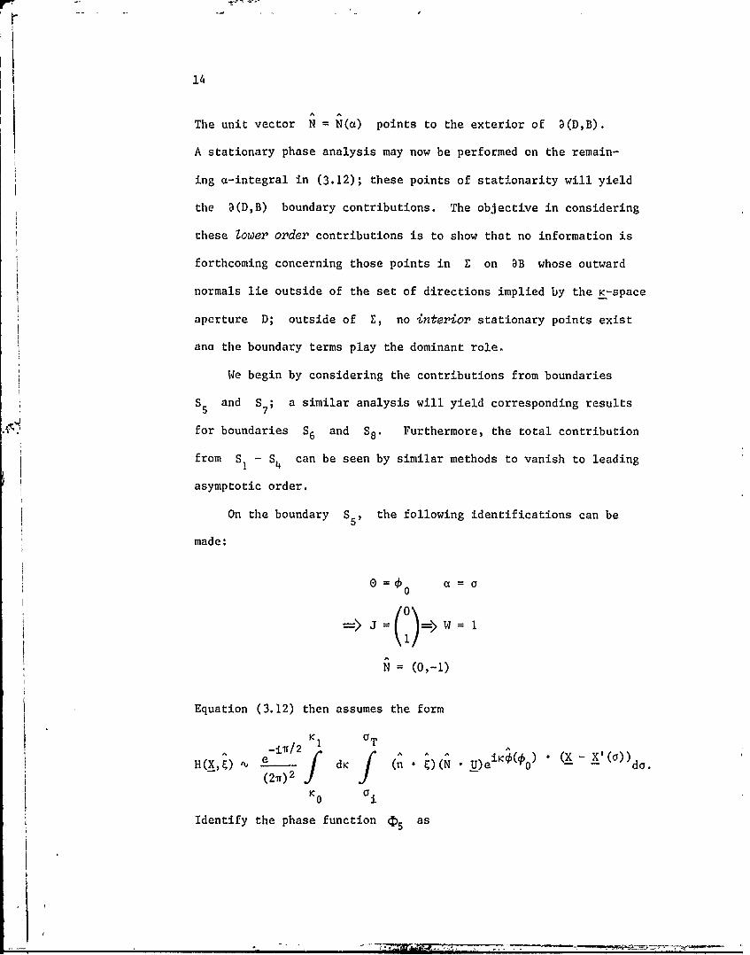
The unit vector N = N(a) points to the exterior of D(D,B).

A stationary phase analysis may now be performed on the remain-

ing a-integral in (3.12); these points of stationarity will yield

the a(D,B) boundary contributions. The objective in considering

these lower order contributions is to show that no information is

forthcoming concerning those points in Z on 3B whose outward

normals lie outside of the set of directions implied by the K-space

aperture D; outside of E, no interior stationary points exist

ana the boundary terms play the dominant role.

We begin by considering the contributions from boundaries

S5 and S7; a similar analysis will yield corresponding results

for boundaries S. and S8 . Furthermore, the total contribution

from S - S can be seen by similar methods to vanish to leading

asymptotic order.

On the boundary S5, the following identifications can be

made:

0= a= a0

=> J= 0 =w

N (0,-1)

Equation (3.12) then assumes the form

-iv/2 K1 [T i

H(~g ~'.--( dK (n - Z)~r UI)e r0 ''do.(27)2 f J

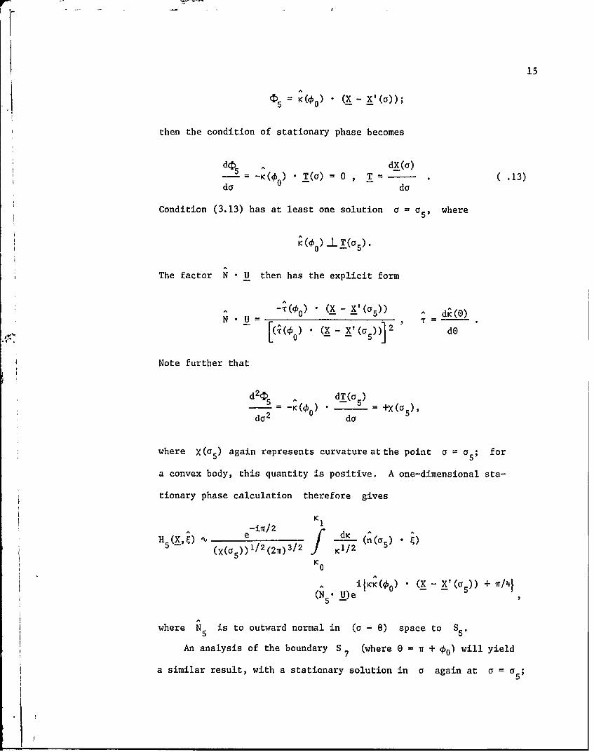
K 0 0I0 ciIdentify the phase function 5as

15

) x - x'()) ;

then the condition of stationary phase becomes

dc5 dX(a)- ,(0) • (o) : 0 , T- ' (.13)

do 0 do

Condition (3.13) has at least one solution a = a., where

( O 5)(as).

The factor N • U then has the explicit form

A

A -T ( 0 ) (X X'(05)) A d (O)N •U: , T:•(X X- X(a))] 2 dO

Note further that

d2c 5 dT(o)5 K(o) 5 +X(s)do2 do

where X(a5) again represents curvature at the point a = a5; for

a convex body, this quantity is positive. A one-dimensional sta-

tionary phase calculation therefore gives

KA -i7T/2 A

H (X, ) e d (n(a) .(Xad) 1/2 (21) 3/2 I K/2

K0

ijKK( o ) (X - X'( )) + I/(N .U)e

where N5 is to outward normal in (a - 8) space to S5.

An analysis of the boundary S (where 0 = w + 00) will yield

a similar result, with a stationary solution in a again at a = a5;

16

the only distinction in this case is that now

^(ii + =

and

(N.U) =-(N•U)5- 7-

The sum of the leading order contributions from s5 and s7,

therefore, gives

H2 ^ (n(c) (NS)(" R((A)-5 1 (x %s) ) 1/ 2(27) 1/2

Sin ,;) • (Z X- z 0()) + 1T/41

f K 1/2

and by integration by parts (retaining only the leading order term)

(n(%) • (5 (oH (X, )"---- -

( 1/2)) /(2?r) 3/2

5.

CosIcK( o) • (X - x'(c)) + 3/.14(3.14),:1%'(,/o) • x - x'(a))

0 0

The principal point to be concluded from an examination of (3.14)

is that (in the exterior of the region Z as identified in Figure

(2.2)) H(K.,) exhibits to leading order a peaking behavior with

central lobe occurring in the vicinity of the line

17

* CX -X() 0

where

*T(G) 05

however, H(X, ) give~s no information concerning the target surface

in this region.

1.8

Appendix A.

In this section, we present a brief derivation of the

POFFIS identity for acoustical wave propagation; the

electromagnetic (vector) case has been outlined by Lewis [3].

As indicated in figure (A.1), we illuminate the acous-

tically hard or soft scatterer B from a time-harmonic point

source located at X0. The incident field UI is thus given

by

eikjX - X_ IUl(X,k) ikie -(A.I)

41Tlx - xo I

and the total acoustic field U is the sum of the incident UT I

and a back-scattered field U, which is also measured at theS

point X

U U + US . (A.2)

The total acoustic field U is required to satisfy the (time-T

reduced) acoustic wave equation with source at X = XO

(V2 + k2)UT = -6(X - X . (A.3)

In addition, we require that UT satisfy an outgoing radiation

condition at infinity, and one of the two boundary conditions

DU T

-=0 xcB (+) , (A.4)3n

or

;t

19

U = 0 X B (-) (A.5)T

The first (+) boundary condition models B as an acoustically

hard reflector; the second (-) condition is the acoustically

soft case. Using (A.1) - (A.5) and the requirement that US

also be outgoing at infinity, one may write a Kirchoff integral

expression for US.

BG(l V) aUSX',k)U (X ,k) s(X',k) - G(X - X') S' , (A.6)s lU an' an'

3B

where the integration is performed over the surface (denoted 3B)

of the scatterer B . In this expression, G(X) is the free-space

outgoing Green's function given by

eikijiG X) (A.7)

We now make a crucial assumption concerning the integrand of (A.6).

Under the integration sign appear the unknown surface field U andDU5 S

the normal derivative - . The physicaZ optics approximation re-S

lates US and - to the incident field U on the surface ofan I

the scatterer by

U S N - U I X e L

au S5

an an

(A.8)

aUsS Xn

ta

20

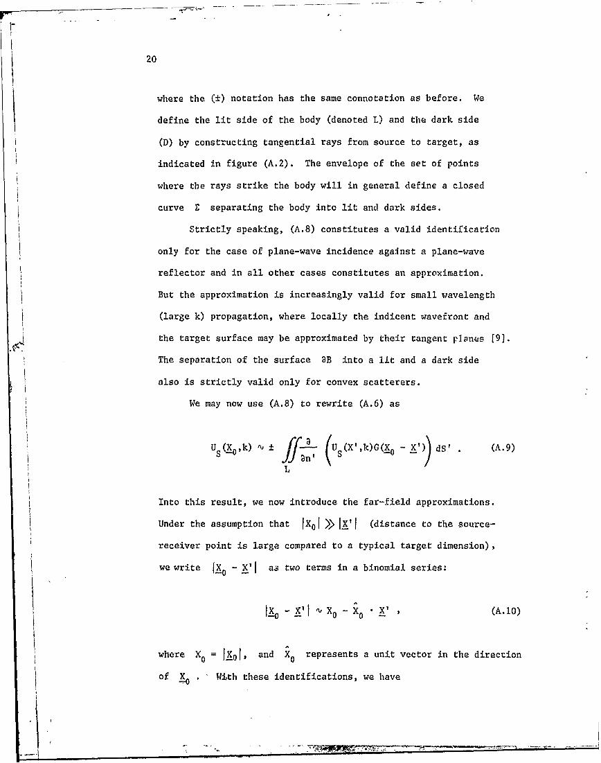
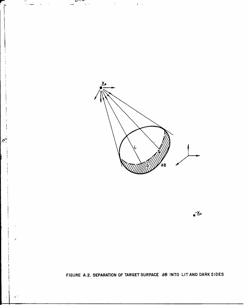
where the (±) notation has the same connotation as before. We

define the lit side of the body (denoted L) and the dark side

(D) by constructing tangential rays from source to target, as

indicated in figure (A.2). The envelope of the set of points

where the rays strike the body will in general define a closed

curve E separating the body into lit and dark sides.

Strictly speaking, (A.8) constitutes a valid identification

only for the case of plane-wave incidence against a plane-wave

reflector and in all other cases constitutes an approximation.

But the approximation is increasingly valid for small wavelength

(large k) propagation, where locally the indicent wavefront and

the target surface may be approximated by their tangent p]anes [9].

The separation of the surface 9B into a lit and a dark side

also is strictly valid only for convex scatterers.

We may now use (A.8) to rewrite (A.6) as

Us(Xo,k) U± /L - (Us(X?,k)G(X - V dS' (A.9)

1J

Into this result, we now introduce the far-field approximations.

Under the assumption that 1X0 1 >>1'I (distance to the source-

receiver point is large compared to a typical target dimension),

we write as0 - aa two terms in a binomial series:

Ix- ' - " X 0 (A.10)

where X= X0 , and X0 represents a unit vector in the direction

of • With these identifications, we have

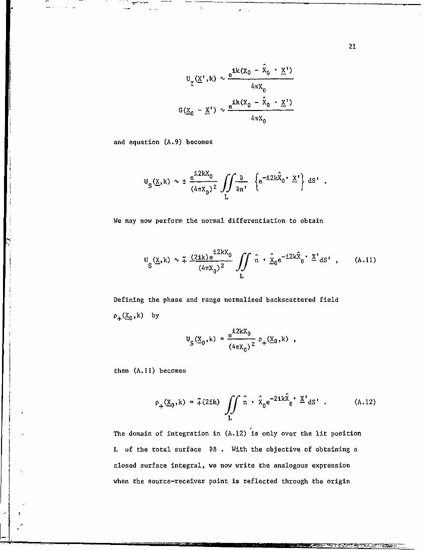
21

U (Xk) e ik(Xo - X0

eik(X 0 X0 )

G(Xo - X') 4X 0

and equation (A.9) becomes

Us (X,k) ' + ( le- 0" dS'S (4Xn)2 '

L

We may now perform the normal differentiation to obtain

U (X,k) o ; (2ik)ei2kX ff n 0e-12kX0 VdS' (A.1)

S - (4rXo)2 -d'

L

Defining the phase and range normalized backscattered field

p+(Xo,k) by

US( k) ei2kXO(4iTX 0) 2 P+(X 0 'k )

then (A.11) becomes

ff ~ -21kx X

p+(X0 ,k) = ;(2ik) n • Xe 0 x dS' (A.12)

L

The domain of integration in (A.12) is only over the lit position

L of the total surface 3B . With the objective of obtaining a

closed surface integral, we now write the analogous expression

when the source-receiver point is reflected through the origin

4 __

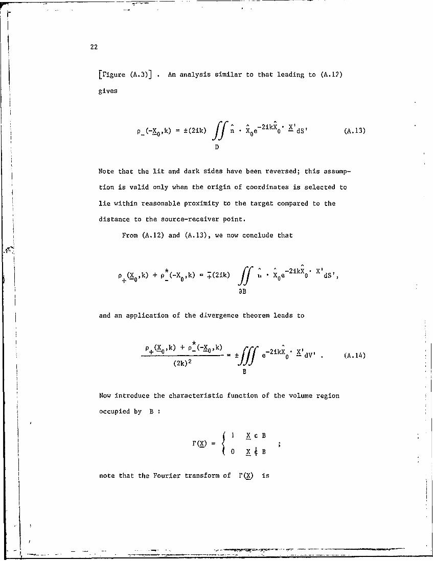
22

[Figure (A.3)] . An analysis similar to that leading to (A.12)

gives

p_(-_X0,k) = ±(21k) n • 0e 2 1k -0 dS' (A.13)

D

Note that the lit and dark sides have been reversed; this assump-

tion is valid only when the origin of coordinates is selected to

lie within reasonable proximity to the target compared to the

distance to the source-receiver point.

From (A.12) and (A.13), we now conclude that

p*-X A/ ^ _21iX

p+(X0,k) + p (-X ,k) -(2ik) t • fe • X'd

3B

and an application of the divergence theorem leads to

f(-jff e-2 ikX " --dV' . (A.14)

(2k)2 JJJB

Now introduce the characteristic function of the volume region

occupied by B

I XcB~r(x) =

note that the Fourier transform of r(X) is

4 - -

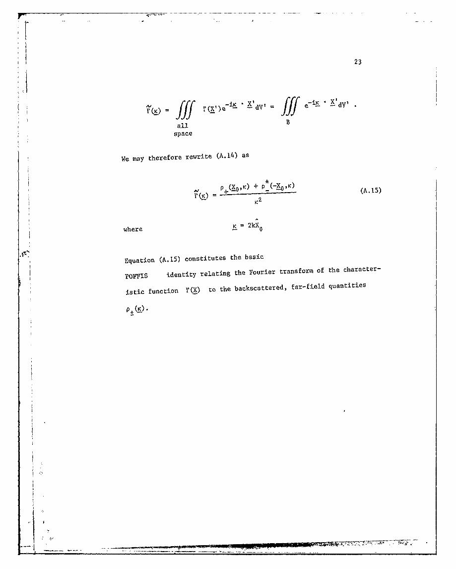
23

r/ .E'dv, e/// - .X'W

r(K) fff rei_ 'c-i fff iS dr

all B

space

We may therefore rewrite (A.14) as

N P+(XOK) + P*(-XK)r(K) --(A15

IC

where K 2kX0

Equation (A.15) constitutes the basic

POFIS identity relating the Fourier transform of the character-

istic function r(x) to the backscattered, far-field quantities

p_ (K:_).

I

P 4

L'

24

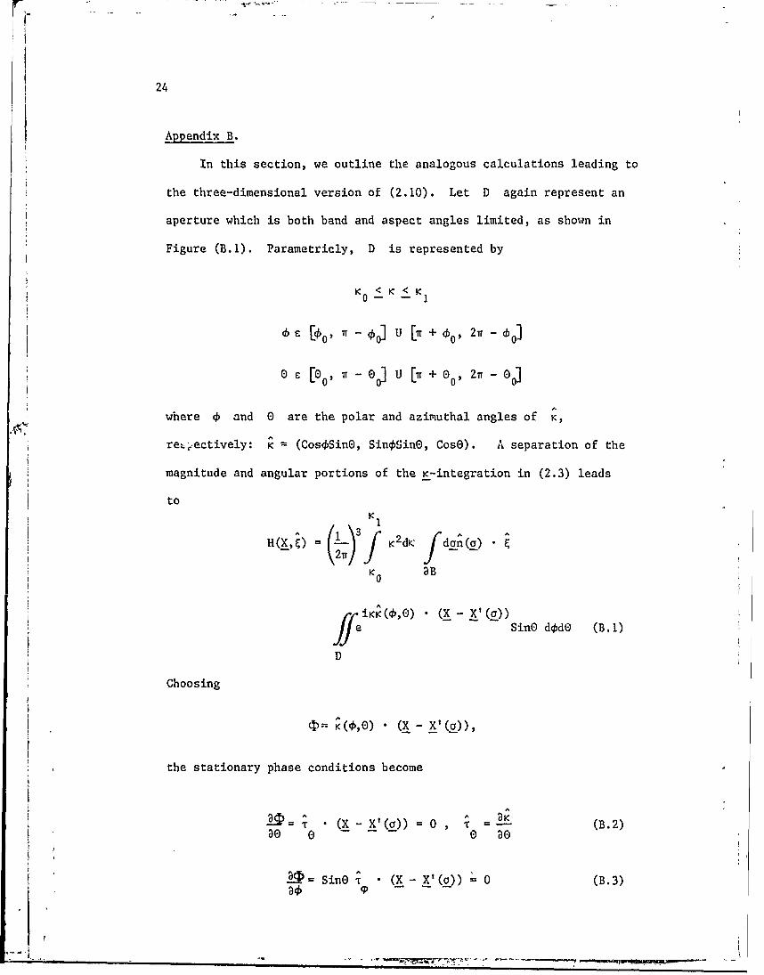
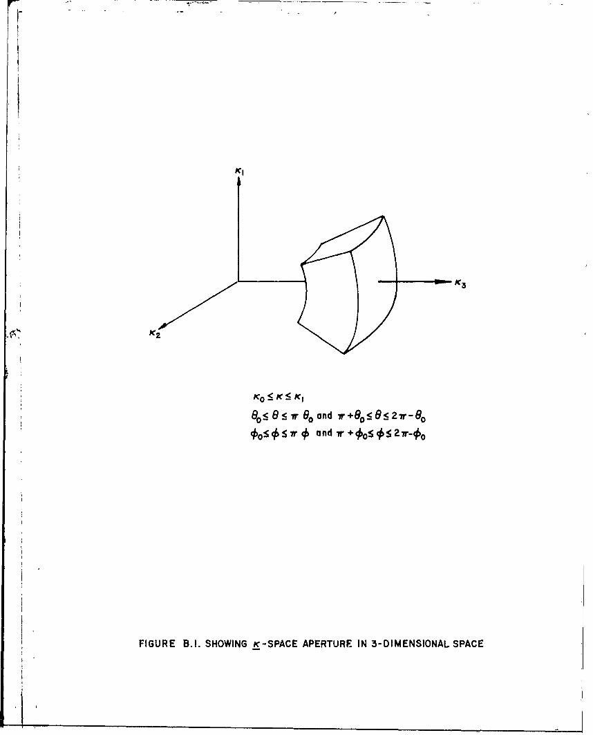
Appendix B.

In this section, we outline the analogous calculations leading to

the three-dimensional version of (2.10). Let D again represent an

aperture which is both band and aspect angles limited, as shown in

Figure (B.1). Parametricly, D is represented by

K0 < K < K,

6C [0' , r - U [Tr + b0 , 27 - o ]

0 [e0, 7- ] U [T + 0o, 2n - o]

where a and e are the polar and azimuthal angles of K,

reLectively: K = (Cos4Sine, Sin4?SinO, CosS). A separation of the

magnitude and angular portions of the K-integration in (2.3) leads

toK

H(X, ) = ( - 2d ono_

0

fiKK(0,0) (X - X'(o))fe SinG dd (B.1)

D

Choosing

?- K (',e) (X - _ )

the stationary phase conditions become

T= • (X - X'(o)) =0, T = (B.2)30 0 0 30

cb =Sine S^ (X - X'(o)) 0 (B.3)

.. ..

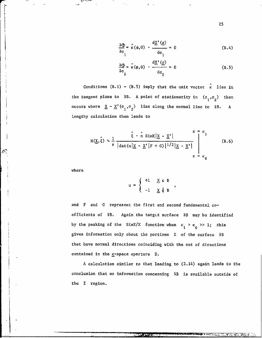
25

A dX' (a)ID= , - = - 0 (B.4)

dol

dX'(a)-- = (4 , • - -- = 0 (B.5)

do 2

Conditions (B.1) - (B.5) imply that the unit vector K lies in

the tangent plane to 3B. A point of stationarity in (oa2) then

occurs where X - X'(o ,1 a2) lies along the normal line to DB. A

lengthy calculation then leads to

A K K1•n SinKLX_ - 1',1H (X, 9) Ou - (B.6)

Idet(uLX- X'[F + G)11/2X-

K K 0

where

-I XcB

and F and G represent the first and second fundamental co-

efficients of B. Again the targct surface 3B may be identified

by the peaking of the SinX/X function when K > K >> 1; this1 0

gives information only about the portions E of the surface 3B

that have normal directions coinciding with the set of directions

contained in the K-space aperture D.

A calculation similar to that leading to (2.14) again leads to the

conclusion that no information concerning 3B is available outside of

the E region.

References

1. Bojarski, N.N., 1967, "Three-dimensional electromagnetic short-pulse inverse scattering", Syracuse University ResearchCorporation, Syracuse, New York.

2. Lewis, R.M., 1969, "Physical optics inverse diffraction",IEEE Transactions in Antennas and Propagation, AP-17,308-314.

3. Perry, W.L., 1974, "On the Bojarski-Lewis inverse scatteringmethod", IEEE Transactions on Antennas and Propagation,AP-22, 6, 826-829.

4. Tabbara, W., 1973, "On an inverse scattering method", IEEETransactions on Antennas and Propagation, AP-21, 245-247.

5. , 1975, "On the feasibility of an inverse scatteringmethod", IEEE Transactions on Antennas and.Propagation,AP-23, 446-448.

6. Rosenbaum-Raz, S., 1976, "On scatterer reconstruction from far-field data", IEEE Transactions on Antennas and Propagation,AP-24, 66-70.

7. Greenspan, D., and Werner, P., 1966, "A numerical method forthe exterior Dirichlet problem for the reduced wave equa-tion", Arch. Ration. Mech. Anal., 23, 288-316.

8. Bleistein, N. and Handelsman, R.A., 1975, Asymptotic Expansionsof Integrals, Holt, Rinehart & Winston, Inc., New York.

9. Majda, A., "High frequency asymptotics for the scattering matrixand the inverse problem of acoustical scattering",to appear.

-'-

r -- -

Exact F.T. of Charact. Physical Optics RelativeWave-Number Function Approx. to Error, %

c) = J1 (2k)k k(~

5 0.02731 0.04292 36.35

10 0.02100 0.01865 12.59

20 0.01980 0.01998 .92

30 0.00488 0.00509 4.12

40 -0.00440 -0.00438 .49

. 50 -0.00485 -0.00491 1.26

60 -0.00062 -0.00066 6.50

70 0.00253 0.00255 0.76

80 0.00209 0.00212 1.51

TABLE I

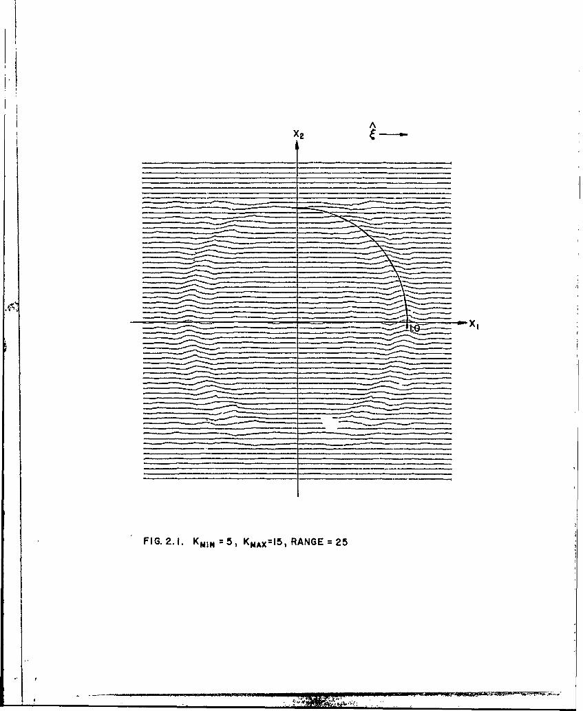
FIG.2.1 KNI = KMXIS)RANE 2

4 - ~ -

-- - ----- -

4-,A

FIG.2.2. KMliN= 10, KMX-3O2 RANGE= 25

X2I

FIG. 2.3. KMIN=I 5 , KMAX= 2 5, RANGE =25

x2

FIG. 2.4. KMIN 15, KMAX: 45, RANGE= 25

V1A

FIG. 2.5. KMNIN =22.5, KvMAx= 3Z.5, RANGE= 25

- ------ X~

FIG. 2.6. KM IN= 10, K MAX= 3 0, RANGE= 25, ALPHA=1200

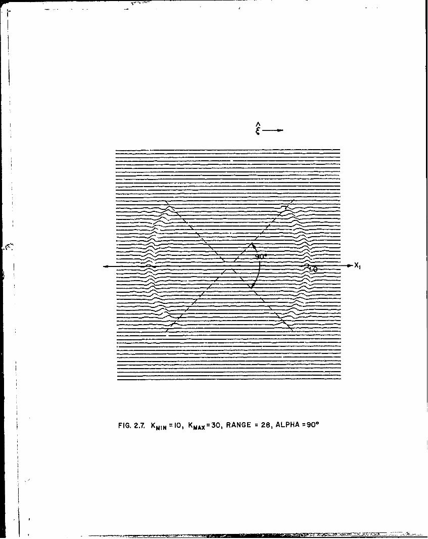
FIG. 2.7. KMIQ 1, KMAX= 30, RANGE= 28, ALPHA =9O*

I-7

FIG. 2.8. KMIN I1 KMAX= 3 0, RANGE 25,ALPHA 600

rr

FIGURE 3.1. SHOWING TWO- DIMENSIONAL. GEOMETRY.

o2 01

FIGURE 3.2 SHOWING THREE DIMENSIONAL GEOMETRY

Ki

F

FIGURE 3.3 BAND AND ASPECT-ANGLES LIMITED APERTURE D IN -KSPACE

K (.

T£

B

N.B

t K-

-ol

N % N

FIGURE 3.4. RELATIONSHIP BETWEEN ZON aB AND K-SPACE APERTUREOF VIEWING DIRECTIONS.

S5 S4

S6 S

S2 S,

FIGURE 3.5. THE BOUNDARY a(D)B) INo 8- SPACE.

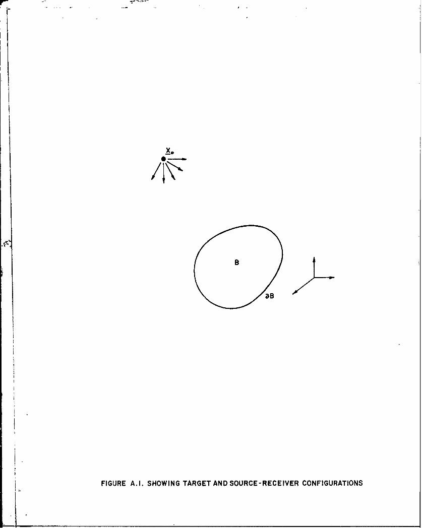
K FIGURE A.I1. SHOWING TARGET AND SOURCE-RECEIVER CONFIGURATIONS

F TB

FIGURE A.2. SEPARATION OF TARGET SURFACE aB INTO LIT AND DARK S IDES

K1

K3

805e8:5r 80 and r +80:58:52 r 80S#0 j:5 r# a nd 7r+0:~ ~ 2 7r- 0 0

FIGURE B.I. SHOWING K-SPACE APERTURE IN 3-DIMENSIONAL SPACE

SECURITY CLASSIFICATION OF THIS PAkGE (WIhen Does Entered)

I RPOR NUBER2. GVT CCESIO NO .YOCSI ICN' ATO N UMBENRD

I4. DTI UT n STATEMENT (oftha epri

disAproautio tis uLimitedAetr Polmo

Phyica DS IUTO tc STTEEN (fitel Ibtecnersedn Bck20. i irn foe, 4.Repor M OO.R)RTNME

44i76-C-74-4-00?\I. SPERMNORAIAINNM AN ADRS 0 OGAELMN.P JI ,T K

1UnieY Orsit (ofj D evere NRgde36 Ifn06ayen de20l b lok75 b,

Inverse arhInsttt Acoustics-0-7

PhyicalfNaa Optiseac EIeragn80imith Aprurc Band-liu"1mting XV

14a*. MRIGAENYNM &.h limit e i pertrn problm ofr phyica15 opUTi Y inveSe satti eri g

Targe dcmyLa beopeel ideptifed fro anli rals anf sale uny itndlimtitio data uiftedr.in fveigage aelmtdaelti

1how DIThT STTEMN targe surfac "ed an beac Itdified fre ep t areomlle

19. ~ ~ ~ ~ ~ ~ ECRT CLKSFIATO OFRD THISirv PAG terseen olt* Inte ed)sr dRe yblc ubr

Inverse4& 7511rn AostcPhysial OticsElectomagetie

SECURITY CLASSIFICATION or THIS PAGE (W*hen Deta Enterod)

... :is available. It is shown that this phenomenon is totally a feature of theFourier transform of characteristic (one-zero) functions and independent ofthe inverse scattering formalism. Numerical examples are given for the caseof a perfectly reflecting circular cylinder.

UNCLASSIFIEDSECURITY CLASSIFICATION OF THIS PAGE(Whan Dala Enterod)